The Markov Theorem for transverse knots

Let $K$ be a transverse closed braid and let $K^{\prime}$ be a preferred longitude for $K$, with $\beta(K)=\beta(K^{\prime})$. We may assume that $K^{\prime}$ is also a transverse closed braid by the transverse Alexander’s Theorem. In this section we focus on the second part of the isotopy of the transverse Markov Theorem, in which we push $K$ across an embedded annulus to $K^{\prime}$. In order to proceed we need to understand better the geometry of the annulus bounded by $K$ and $K^{\prime}$.

Because $K^{\prime}$ is a preferred longitude for $K$, they bound an embedded annulus $\cal{A}$. This annulus is a subsurface of a Markov surface for $K$. In this section, we will extend some of Birman’s and Menasco’s results about the foliated surface to the transverse setting and use these results to simplify the foliation of $\cal{A}$. The simplification consists of the transverse moves on the boundary braids $K$ and $K^{\prime}$ as described in Lemma 2, and changes in foliation on the interior of the surface as described in Section 2. Our goal for now is to simplify the foliated annulus enough to describe its embedding completely. Following the methods described in Section 2, we divide our work among the three types of tiles.

Remark: In the annulus the surface will be to the left of $K$, and to the right of $K^{\prime}$, while all of the moves guided by the surface have been described in Section 2 for the case when the surface is to the left of the braid. The braid being to the right of the surface simply changes the sign of the braid moves being guided by the surface. For example, even though only positive stabilizations are transverse and the $ab$-tiles that guide these moves are negative for $K$ (as described in Section 2), for $K^{\prime}$ a positive stabilization is guided by a positive $ab$-tile.

We will now describe the foliation that results from these simplifications. In a later section we will describe the embedding of the annulus, which will allow us to further simplify the foliation.

Proof: We start our with the $aa$-tiles. Each closed $aa$-tile is bounded by a trivial loop in either $K$ or $K^{\prime}$, with the sign of the trivial loop of $K$ corresponding to the sign of the tile and the sign of the trivial loop of $K^{\prime}$ the opposite of the tile’s sign. Depending on the sign of the tile, we may be able to transversely (positively) destabilize the braid along the tile to get rid of the vertex and singularity. We can destabilize $K$ if the tile bounded by $K$ is positive, and $K^{\prime}$ if the tile bounded by $K^{\prime}$ is negative. After we have transversely destabilized $K$ and $K^{\prime}$ along as many of the $aa$-tiles as possible, we are left with some number of closed negative $aa$-tiles along $K$ and some number of closed positive $aa$-tiles along $K^{\prime}$. Using the $aa$-exchange moves described in Section 2, we can push the $aa$-tiles along each boundary until they are all in the same spot, forming a tab from $K$ and $K^{\prime}$. Recall Figure 6. It will be useful later on to consider the braids $K$ and $K^{\prime}$ minus these tabs of $aa$-tiles. Although they will not be the same transverse knot type as $K$ and $K^{\prime}$, they will be the same topological knot type.

Along each braid there will be some number of positive and negative $ab$-tiles. We first eliminate pairs of oppositely signed tiles that share a common $a$-arc and a common $b$-arc by performing $ab$-exchange moves along $K$ or $K^{\prime}$, as described in Section 2. Recall Figure 8. If there are any $ab$-tiles along $K$ or $K^{\prime}$ that share a common $b$-arc and have the same sign, then we may reduce the valence of their common vertices by using a change in foliation. Recall Figure 11. Depending on the sign of the tiles, we may stabilize $K$ or $K^{\prime}$ further along the modified $ab$-tiles. If there are any other negative $ab$-tiles along $K$, we may transversely remove them by positively stabilizing $K$ along those tiles. In the same way, we may get rid of any other positive $ab$-tiles along $K^{\prime}$ by positively stabilizing $K^{\prime}$ along them, noting that the sign is correct because $K^{\prime}$ is to the right of the surface. Recall Figure 2. We conclude that after some number of $ab$-exchange moves and $aa$-exchange moves, positive stabilizations, and changes in foliation, along $K$ we are left with only positive $ab$-tiles that share an $a$-arc and the tab of negative $aa$-tiles constructed above, and along $K^{\prime}$ we have negative $ab$-tiles sharing an $a$-arc and the tab of positive $aa$-tiles.

To complete our description of the foliated annulus, we need some lemmas and terminology from [BF98]:

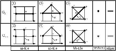
The following results hold for embedded surfaces bounded by a braid, but by Lemma 2, they are also true for an embedded surface with transverse boundary.

Let $\vec{x}=x,\dots,x$, where $x$ is a sign $+$ or $-$.

We complete our description of the foliation of the interior of the surface with the following lemma.

Proof: We will prove the claim for the case when the vertex is negative. If a negative interior vertex $v$ has valence 1 in the graph $G_{--}$, then it is an endpoint of the graph. By Lemma 8, after performing some number of exchange moves, changes in foliation, and braid isotopies, we may assume that $v$ is not the endpoint of $G_{--}$, so does not have valence 1 in the graph.

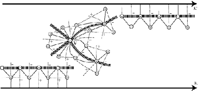
If an interior vertex has valence greater than 2 in the graph , then there is some branching of the graph at $v$. See Figure 15. After some number of exchange moves, changes in foliation, and braid isotopies, the graph $G_{--}$ does not have endpoints on $K$ or $K^{\prime}$, or at any interior vertex, so it must be a closed graph. If there is branching, then only one of the branches closes up to form a curve that is parallel to the boundary and all other branches close up as the boundary of discs. By Lemma 9, after some number of exchange moves, changes in foliation, and isotopies in the complement fo the axis, we may assume that no closed loop of $G_{--}$ bounds a disc. Therefore, there is no branching, so no negative interior vertex in the graph has valence greater than 2.

The proof of the lemma is complete when we observe that the graph $G_{++}$, after some number of exchange moves, changes in foliation, and braid isotopies, also has no endpoints on $K$ or $K^{\prime}$ so the results above about $G_{--}$ and negative interior vertices is also true for $G_{++}$ and positive interior vertices. $\|$

To conclude that the surface is foliated as in Figure 12, we perform more changes in foliation, exchange moves, and isotopies in the complement of the axis until we can assume that for each interior vertex $v$, the singularities in $star(v)$ alternate sign (Lemma 7). Since by the above lemma we know that each interior vertex has exactly two positive or two negative vertices, this is enough to conclude that the valence of each interior vertex in the surface is 4, and our foliation has the claimed form. The proof of the proposition is complete. $\|$

An example of a foliated annulus with all interior vertices having valence $2$ in the graphs is pictured in Figure 12. Although we didn’t know at the beginning of this section how many positive $ab$-tiles and negative $ab$-tiles there are in the foliated annulus, from the configuration of the $bb$-tiles we see that there must be the same number of each.

We may use our results about the foliation to conclude that the braid index of $K$ must be the same as the braid index of $K^{\prime}$, modulo the tab of $aa$-tile bounding trivial loops coming off of each (see Figure 12). For in terms of the surface bounded by the braid, the braid index of the boundary braid is the algebraic intersection number of the axis with the surface. This gives a formula for the braid index of the braid from its foliated surface: $b(K)=$ #(positive vertices)$-$ #(negative vertices). We already have the Markov surface ${\cal F}$ for $K$, and we may isotope the Markov surface for $K^{\prime}$ to ${\cal F}-{\cal A}$, the subsurface of ${\cal F}$ that is the complement of the checkerboard annulus. Then the difference between $b(K)$ and $b(K^{\prime})$ is the difference #(positive vertices)- #(negative vertices) in the annulus ${\cal A}$, which is 0, modulo the vertices in the $aa$-tiles. We shall see later that in fact there is the same number of positive and negative $aa$-tiles.

We have shown that, after some number of changes in foliation, exchange moves, transverse stabilizations and destabilizations of $K$ and $K^{\prime}$, we may assume that the foliation of the annulus they bound has the checkerboard pattern pictured in Figure 12. In fact, it suffices to prove the TMT for preferred longitudes for the case when the foliation has an even simpler pattern: a checkerboard with no $bb$-tiles. See Figure 16. For if we can push $K$ across this simplified annulus to $K^{\prime}$, then we may inductively work across the rest of an annulus with $bb$-tiles in the pattern of Figure 12.

It is here that the modification of the Birman-Menasco proof reaches a difficulty. In the non-transverse setting, we may destabilize $K$ and $K^{\prime}$ along the $ab$-tiles and stabilize them along the $aa$-tiles, giving us a nonsingularly foliated annulus, then we may push $K$ across the remaining surface to $K^{\prime}$. Since none of these moves is transverse, we must attack the foliation differently, by showing that if $K$ and $K^{\prime}$ are transverse preferred longitudes, then the moves we have already performed leave us with a foliation whose $b$-arcs are all inessential. Recall that there is an embedding of the annulus of Figure 16 with all of the $b$-arcs inessential: a piece of it is pictured in Figure 5. The inessential b-arcs in this figure are facing out of the page, between vertices $B$ and $C$. When we consider an extension of this embedding through the rest of the annulus, with all of the $b$-arcs inessential, we will be able to remove the vertex $A$ and the vertex above it, and the vertex $D$ and the vertex below it, and continue in this way through the rest of the foliation. This leaves an annulus which does not intersect the axis at all.

Until now, we have considered the annulus as a single embedded surface with two boundary components, $K$ and $K^{\prime}$. Now we would like to shift our point of view to the graphs $G_{++}$ and $G_{--}$ of the foliation, and describe the annulus as a union of subannuli with these graphs as core circles. In the following, we will use Cromwell’s work on arc-presentations to first decompose the annulus into a union of three subannuli. Then we will prove that this decomposition can always be replaced by a simpler decomposition into a union of two subannuli whose foliation has all inessential $b$-arcs.

Arc-presentations of oriented knot types have been studied by Cromwell, whose paper [Cr95] we closely follow here.

Consider the open-book decomposition of the 3-sphere which has open disks $H_{\theta}$ for pages and an unknotted circle (which we can take as the $z$-axis $\cup$ $\infty$ ) for the binding. A knot can be embedded in finitely many half-planes $H_{\theta}$ so that it meets each half-plane in a single simple arc. Such an embedding is called an arc-presentation of the knot. Cromwell proves that every oriented link type has an arc-presentation. We will be concerned with arc-presentations of oriented knots.

As an example, consider the Figure $8$ knot pictured in Figure 17. The knot diagram pictured in Figure 17 is easily turned into an arc-presentation. There are many ways to obtain an arc-presentation from a given braid diagram; they are detailed in [Cr95] and [Cr96].

An arc-presentation for an oriented knot type $\cal{K}$ is determined (up to equivalence by a sequence of moves described in Section 4.3) by two sets of data: the cyclic list of points of intersection of the knot with the $z$-axis, ordered with respect to increasing $z$ and listed as one traverses the knot once, and the cyclic list of half planes each arc appears in, ordered with respect to $\theta$ and again listed as one traverses the knot. In the example in Figure 17, the arc-presentation is given by the permutations $(1,5,3,6,2,4)$ and $(6,3,5,1,4,2)$ ordering the intersections and half-planes, respectively. The data describing an arc-presentation in this way corresponds directly to the ordered lists of vertices and singularities obtained from traversing one component of the graph $G_{++}$ or $G_{--}$ of the embedded simplified annulus that we described in Section 4.1. In fact, the data that describe $G_{++}$ and $G_{--}$ determine $G_{++}$ and $G_{--}$ as an arc-presentation of $\cal{K}$.

By Lemma 11, for the rest of this section we may assume that our surface has been isotoped so that the graphs $G_{++}$ and $G_{--}$ are arc-presentations for $\cal{K}$. We can associate a braid to an arc-presentation in a simple way. At each point of intersection of the arc-presentation with the axis, push the arc-presentation off of the axis in the direction that is normal to the plane spanned by the tangent along the (oriented) arc and the axis. There is a choice of two directions; choose the normal that makes the positive frame with the tangent and the axis. Then orientation of the pushed off curve will be positive with respect to $\theta$. Traveling along the rest of the curve we may push slightly off of the arc-presentation in the same direction, so that the resulting curve is a braid. This pushoff would be the inverse of the isotopy $h$ used in the proof of Lemma 11. If we push off in the other direction from the axis and along the arc-presentation, we have an anti-braid. An anti-braid is a knot that satisfies all of the definitions of a closed braid except that it is increasing with respect to $-\theta$ rather than $\theta$. We call these knots the braid and anti-braid associated to the arc-presentation. See Figure 18. (There is an ”anti-Markov” theorem for anti-braids, which uses anti-braid isotopy and the Markov moves of type II and III along with stabilization and destabilization, all of which are oriented in the opposite direction from the moves of the Markov Theorem for braids).

We use the associated braids and anti-braids of the graphs $G_{++}$ and $G_{--}$ to decompose the annulus into a union of three subannuli. Given the arc-presentations $G_{++}$ and $G_{--}$ lying in the annulus $\cal{A}$, we can push them off of the axis towards the boundary of the annulus to form two closed braids. By construction, we may take these braids to be $K$ and $K^{\prime}$ minus their tabs of negative $aa$-tiles and positive $aa$-tiles, respectively. We can also push the arc-presentations off of the axis in the other direction into the annulus to obtain two closed anti-braids, $K_{0}$ and $K^{\prime}_{0}$. In this way, we have a decomposition of $\cal{A}$ into three subannuli: one with core circle $G_{++}$, whose boundary components are the braid $K$ and an anti-braid $K_{0}$, one with core circle $G_{--}$, whose boundary components are the braid $K^{\prime}$ and an anti-braid $K^{\prime}_{0}$, and a nonsingularly foliated center annulus, whose boundary components are the anti-braids $K_{0}$ and $K^{\prime}_{0}$. These annuli intersect along the boundary anti-braids. See Figure 19.

Now we wish to consider the isotopy of the anti-braid $K_{0}$ to the anti-braid $K^{\prime}_{0}$ that is guided by the nonsingular subannulus of $\cal{A}$ between $K_{0}$ and $K^{\prime}_{0}$. Recall Figure 19. The facts that the annulus is nonsingular between $-K_{0}$ and $-K^{\prime}_{0}$ (so $-K_{0}$ and $-K^{\prime}_{0}$ have the same braid index,) implies that the isotopy between $-K_{0}$ and $-K_{0}$ is a braid isotopy in the complement of the braid axis. The isotopy of $-K_{0}$ corresponds to an isotopy of $K_{0}$, so we conclude that the anti-braids $K_{0}$ and $K^{\prime}_{0}$ are also related by anti-braid isotopy in the complement of the axis.

In [Cr95] Cromwell defined a set of moves that relate two different arc-presentations of the same oriented knot type. See the thick black curves in Figures 21, 22, and 20. He proved that any two arc-presentations of the same oriented knot type are related by a finite sequence of the moves from this set.

There is a similar move of type $i(b)$ (Figure 21,) with oppositely signed crossing. The sign of the crossing depends on the $\theta$-order of the planes involved. Note that the type $ii$ move (Figure 22,) is possible only when the arcs coming into and out of the two vertices are not in alternating $\theta$-planes. When looking down the axis at the arc-presentation, this condition is the same as requiring that the arcs through these vertices, though touching at the axis, do not cross.

Because $K_{0}$ and $K^{\prime}_{0}$ are braid isotopic, we may choose an isotopy of $K_{0}$ across the annulus to $K^{\prime}_{0}$ that leaves $K$ and $K^{\prime}$ fixed. Because $G_{++}$ is isotopic to $G_{--}$ across a nonsingular annulus, we may also choose an arc-equivalence of $G_{++}$ and $G_{--}$ that fixes $K$ and $K^{\prime}$.

The essence of this proof is to consider the arc-equivalence under the restrictions that the annulus ${\cal A}$ must remain embedded, and that the boundary components $K$ and $K^{\prime}$ of ${\cal A}$ must be preserved. Therefore, in Figures 21, 22, and 20 below, we are looking at changes in the arc-presentation, braid, and anti-braid and considering the embedding of the subannulus bounded by the braid and anti-braid. Although the braids associated to $G_{++}$ and $G_{--}$ are actually $K$ and $K^{\prime}$ minus their negative trivial loops, our examination concerns moves that we may assume are supported away from the loops. Therefore, fixing the braids associated to $G_{++}$ and $G_{--}$ will fix the boundary braids $K$ and $K^{\prime}$. We will look at each of the three possible Cromwell moves of the arc-equivalence from this point of view.

A move of type $i(a)$ or $i(b)$ on $G_{++}$ will stabilize or destabilize either $K$ or $K_{0}$. See Figure 21. If the braid isotopy of $K_{0}$ induced type $i$ moves on $G_{++}$ then there would be an induced stabilization or destabilization of $K$. However, we assumed that the isotopy of $G_{++}$ to $G_{--}$ fixed $K$. We conclude that the arc-equivalence does not include moves of type $i(a)$ or $i(b)$.

In Figure 22, we see that a move of type $ii$ on two vertices of the arc-presentation corresponds to an exchange move of the braid and a vertical isotopy of a piece of the anti-braid, or to an exchange move of the anti-braid and a vertical isotopy of a piece of the braid, or to a vertical isotopy of pieces of both the braid and the anti-braid, depending on the $\theta$-order and orientation of the involved arcs in the arc-presentation. Figure 22(A) shows an exchange move of the anti-braid (gray) and a vertical isotopy of two pieces of the braid (black). Figure 22(B) shows a vertical isotopy of two pieces of the anti-braid (gray), and a vertical isotopy of two pieces of the braid (black).

Neither $K$ nor $K_{0}$ admit exchange moves, so if the arc-equivalence includes a type $ii$ move then there is a corresponding vertical isotopy of pieces of $K$ and $K_{0}$, as in Figure 22(B). However, such a vertical isotopy would cause the subannulus bounded by $K$ and $K_{0}$ to intersect itself. We conclude that the arc-equivalence does not include a type $ii$ move.

Ruling out moves of type $i$ and $ii$, we are left only with the moves of type $iii$. $\|$

Since the isotopy of $K_{0}$ to $K^{\prime}_{0}$ does not change the anti-braid word, we can identify them as a single anti-braid $K_{0}$. We get a simpler decomposition of the annulus from this identification of the two anti-braids, just like the one in Figure 19, except that the single anti-braid $K_{0}$ is the common boundary of the two subannuli. In this identification, we see that the $b$-arcs connecting the vertices of the arc-presentations traced the trivial shift of $K_{0}$ to $K^{\prime}_{0}$, so are inessential. Therefore, the embedding of the annulus bounded by $K$ and $K^{\prime}$ is like that pictured in Figure 5, with all inessential $b$-arcs.

Using this embedding, we may now prove the following proposition:

Proof: Let us modify the surface to remove all of the inessential $b$-arcs, as in Figure 5. This modification removes all of the singularities and vertices from the foliation, except for the tab of negative $aa$-tiles bounded by negative trivial loops of $K$ and the tab of positive $aa$-tiles bounded by negative trivial loops of $K^{\prime}$. We can now push $K$ transversely across the nonsingular annulus and positively stabilize it across the positive $aa$-tiles bounded by $K^{\prime}$, and we can push $K^{\prime}$ transversely across the annulus and positively stabilize it across the negative $aa$-tiles bounded by $K$. This leaves us with a nonsingular foliation of $\cal{A}$. We conclude that there is a transverse braid isotopy that takes $K$ across the nonsingular annulus to $K^{\prime}$. $\|$

References

- [Be83] D. Bennequin, Entrelacements et équations de Pfaff, Astérisque 107-8 (1983), 87-161. English version: Russian Math. Surveys 44, No. 3 (1989), 1-65. Section numbers in the two versions agree.
- [BM90] J.S. Birman and W. Menasco, Studying links via closed braids IV: Composite and split links, Invent. Math. 102 (1990), 115-139.
- [Sw92] J. Swiatkowski, On the isotopy of Legendrian knots, Ann. Glob. Anal. Geom., 10 (1992), pp 195-207.
- [BM94] J. S. Birman and W. Menasco, Special positions for essential tori in link complements, Topology, 33, No. 3 (1994), 525-556. See also Erratum, Topology, 37, (1998), No. 1, page 225
- [Cr95] P.R. Cromwell, Embedding knots and links in an open book I: Basic properties, Topology and its Applications 64 (1995) pp 37-58.
- [Cr96] P.R. Cromwell and I.J. Nutt, Embedding knots and links in an open book II: Bounds on arc index, Math. Proc. Camb. Phil. Soc. 119 (1996) pp 309-319.
- [FT97] D. Fuchs and S. Tabachnikov, Invariants of Legendrian and transverse knots in the standard contact space, Topology, 36, (1997), No. 5, 1025-1053.
- [BF98] J. S. Birman and E. Finkelstein, Studying surfaces via closed braids, J. Knot Theory Ramifications, 7, No. 3 (1998), 267-334.
- [BW00] J. S. Birman and N. C. Wrinkle, On transversally simple knots, J. Differential Geometry, 55, (2000), pp 325-354.
- [BM02] J.S. Birman and W.W. Menasco, On Markov’s Theorem, Proceedings KNOTS-2000, World Scientific Publishing Company, to appear.