The Automorphism Group of the Complex of Pants Decompositions
1 Introduction
There has been recent interest in finding combinatorial models for groups, i.e. finding a simplicial complex whose automorphism group is a given group. For example, Charney-Davis showed that the Coxeter Diagram is a model for (for certain Coxeter groups W) [3], and Bridson-Vogtmann showed that a spine of Outer Space is a model for [1]. In this paper, we prove that the complex of pants decompositions is a model for the mapping class group.
Throughout, will denote a closed oriented surface of negative Euler characteristic.
The complex of pants decompositions of S, defined by Hatcher-Thurston and denoted , has vertices representing pants decompositions of , edges connecting vertices whose pants decompositions differ by an elementary move (see below), and 2-cells representing certain relations between elementary moves. Its 1-skeleton is called the graph of pants decompositions, and is denoted .
Brock proved that models the Teichmüller Space of endowed with the Weil-Petersson metric, , in that the spaces are quasi-isometric [2]. Our main result further indicates that is the “right” combinatorial model for , in that the automorphism group of is shown to be the extended mapping class group of , (the group of diffeomorphisms of to itself, modulo isotopy). This is in consonance with the result of Masur-Wolf that the isometry group of is [12]. The extended mapping class group has a natural action by automorphisms on ; the content of the theorem is that all of the automorphisms of are induced by elements of .
The Main Theorem of this paper is as follows:
Main Theorem. Let be a closed oriented surface of negative Euler Characteristic which is not the genus surface with punctures. Then:
The two isomorphisms are proved in Sections 4 and 5, respectively. To prove the first isomorphism of the Main Theorem, we show that the 2-cells of , which are defined via topological relations between pants decompositions on , can equivalently be characterized using only the combinatorics of . In other words, carries no more information than its 1-skeleton. For example, square 2-cells of (those representing relations involving four elementary moves) are defined as a commutator relation made up of elementary moves on disjoint subsurfaces on (see Figure 4). We show that square 2-cells can equivalently be defined as loops with 4 edges in which have the property that adjacent edges in the loop do not lie in a common Farey graph (see below) in . Note that in the second definition there is no mention of the surface, only . Therefore, any automorphism of preserves these square 2-cells.
In order to prove the second isomorphism of the Main Theorem, we use the fact that for any satisfying the hypotheses of the Main Theorem, we have the following isomorphism:
where is the complex of curves for (defined below). This isomorphism is a theorem of Ivanov [7]. Korkmaz proved the low genus case [9], and Luo gave another proof for any genus [10].
While has a vertex for each top-dimensional simplex of , it is only a relatively small subcomplex of the dual of , and hence the main result of this paper does not follow from Ivanov’s theorem.
The key idea for the second isomorphism of the Main Theorem is that there is a correlation between marked Farey graphs (see below) in and vertices in . An automorphism of induces a permutation of these Farey graphs, and hence gives rise to an automorphism of . The difficulty is to show that this map between the automorphism groups of and is well-defined.
2 The Complexes
Complex of Curves.
The complex of curves (or curve complex) of is the simplicial complex whose vertices correspond to isotopy classes of nontrivial simple closed curves on ; a curve is nontrivial if it is essential (not null homotopic) and nonperipheral (not homotopic to a boundary component). Throughout, we will use curve to mean isotopy class of curves. Also we will lose the distinction between isotopy classes of curves and representatives of the isotopy classes.
A set of vertices of the curve complex is the -skeleton of a -simplex if the corresponding curves have trivial intersection pairwise (there is a set of representatives of the classes which are mutually disjoint). For example, edges correspond to pairs of disjoint curves, triangles correspond to triples of disjoint curves, etc.
The curve complex was first defined by Harvey [5]. Harer proved that it is homotopy equivalent to a wedge of spheres [4]. Ivanov used his theorem that to give a new proof of Royden’s Theorem that (where is the Teichmüller Space of with the Teichmüller metric) [7]. Masur-Minksy have shown that the complex of curves is -hyperbolic [11].
The complex of curves has an altered definition in two cases. For and ( denotes the genus surface with boundary components), since there are no distinct simple closed curves with trivial intersection, two vertices are connected by an edge when the curves they represent have minimal intersection (2 in the case of , and 1 in the case of ). It turns out that in both cases, the complex of curves is an ideal triangulation of the disk, or Farey Graph (see Figure 1) [13].
xunit=1cm
yunit=1cm
(-3,-3)(3,3)
(0,3)(0,0)(0,-3)
(3.00,0.00)(1.06,1.06)(0.00,3.00) \pscurve(0.00,3.00)(-1.06,1.06)(-3.00,0.00) \pscurve(-3.00,0.00)(-1.06,-1.06)(-0.01,-3.00) \pscurve(-0.01,-3.00)(1.06,-1.06)(3.00,-0.01) \pscurve(3.00,0.00)(2.08,0.86)(2.12,2.12) \pscurve(2.12,2.12)(0.86,2.08)(0.00,3.00) \pscurve(0.00,3.00)(-0.86,2.08)(-2.12,2.12) \pscurve(-2.12,2.12)(-2.08,0.86)(-3.00,0.00) \pscurve(-3.00,0.00)(-2.08,-0.86)(-2.13,-2.12) \pscurve(-2.13,-2.12)(-0.87,-2.08)(-0.01,-3.00) \pscurve(-0.01,-3.00)(0.86,-2.08)(2.12,-2.13) \pscurve(2.12,-2.13)(2.08,-0.87)(3.00,-0.01) \pscurve(3.00,0.00)(2.57,0.51)(2.77,1.15) \pscurve(2.77,1.15)(2.18,1.46)(2.12,2.12) \pscurve(2.12,2.12)(1.46,2.18)(1.15,2.77) \pscurve(1.15,2.77)(0.51,2.57)(0.00,3.00) \pscurve(0.00,3.00)(-0.51,2.58)(-1.15,2.77) \pscurve(-1.15,2.77)(-1.46,2.18)(-2.12,2.12) \pscurve(-2.12,2.12)(-2.18,1.46)(-2.77,1.15) \pscurve(-2.77,1.15)(-2.57,0.52)(-3.00,0.00) \pscurve(-3.00,0.00)(-2.58,-0.51)(-2.77,-1.14) \pscurve(-2.77,-1.14)(-2.19,-1.45)(-2.13,-2.12) \pscurve(-2.13,-2.12)(-1.46,-2.18)(-1.15,-2.77) \pscurve(-1.15,-2.77)(-0.52,-2.57)(-0.01,-3.00) \pscurve(-0.01,-3.00)(0.51,-2.58)(1.14,-2.77) \pscurve(1.14,-2.77)(1.45,-2.19)(2.12,-2.13) \pscurve(2.12,-2.13)(2.18,-1.46)(2.77,-1.16) \pscurve(2.77,-1.16)(2.57,-0.52)(3.00,-0.01) \pscurve(3.00,0.00)(2.80,0.28)(2.94,0.58) \pscurve(2.94,0.58)(2.69,0.82)(2.77,1.15) \pscurve(2.77,1.15)(2.48,1.33)(2.49,1.67) \pscurve(2.49,1.67)(2.17,1.78)(2.12,2.12) \pscurve(2.12,2.12)(1.79,2.17)(1.67,2.49) \pscurve(1.67,2.49)(1.33,2.48)(1.15,2.77) \pscurve(1.15,2.77)(0.82,2.69)(0.59,2.94) \pscurve(0.59,2.94)(0.28,2.80)(0.00,3.00) \pscurve(0.00,3.00)(-0.27,2.80)(-0.58,2.94) \pscurve(-0.58,2.94)(-0.81,2.69)(-1.15,2.77) \pscurve(-1.15,2.77)(-1.32,2.48)(-1.66,2.50) \pscurve(-1.66,2.50)(-1.78,2.18)(-2.12,2.12) \pscurve(-2.12,2.12)(-2.17,1.79)(-2.49,1.67) \pscurve(-2.49,1.67)(-2.48,1.33)(-2.77,1.15) \pscurve(-2.77,1.15)(-2.69,0.82)(-2.94,0.59) \pscurve(-2.94,0.59)(-2.80,0.28)(-3.00,0.00) \pscurve(-3.00,0.00)(-2.80,-0.27)(-2.94,-0.58) \pscurve(-2.94,-0.58)(-2.69,-0.81)(-2.77,-1.14) \pscurve(-2.77,-1.14)(-2.48,-1.32)(-2.50,-1.66) \pscurve(-2.50,-1.66)(-2.18,-1.78)(-2.13,-2.12) \pscurve(-2.13,-2.12)(-1.79,-2.17)(-1.67,-2.49) \pscurve(-1.67,-2.49)(-1.33,-2.48)(-1.15,-2.77) \pscurve(-1.15,-2.77)(-0.82,-2.69)(-0.59,-2.94) \pscurve(-0.59,-2.94)(-0.28,-2.80)(-0.01,-3.00) \pscurve(-0.01,-3.00)(0.27,-2.80)(0.58,-2.94) \pscurve(0.58,-2.94)(0.81,-2.69)(1.14,-2.77) \pscurve(1.14,-2.77)(1.32,-2.48)(1.66,-2.50) \pscurve(1.66,-2.50)(1.78,-2.18)(2.12,-2.13) \pscurve(2.12,-2.13)(2.17,-1.79)(2.49,-1.67) \pscurve(2.49,-1.67)(2.48,-1.33)(2.77,-1.16) \pscurve(2.77,-1.16)(2.69,-0.82)(2.94,-0.59) \pscurve(2.94,-0.59)(2.80,-0.28)(3.00,-0.01) \pscurve(3.00,0.00)(2.90,0.14)(2.99,0.29) \pscurve(2.99,0.29)(2.87,0.43)(2.94,0.58) \pscurve(2.94,0.58)(2.82,0.71)(2.87,0.87) \pscurve(2.87,0.87)(2.74,0.98)(2.77,1.15) \pscurve(2.77,1.15)(2.63,1.24)(2.65,1.41) \pscurve(2.65,1.41)(2.49,1.49)(2.49,1.67) \pscurve(2.49,1.67)(2.33,1.73)(2.32,1.90) \pscurve(2.32,1.90)(2.15,1.95)(2.12,2.12) \pscurve(2.12,2.12)(1.95,2.15)(1.90,2.32) \pscurve(1.90,2.32)(1.73,2.33)(1.67,2.49) \pscurve(1.67,2.49)(1.50,2.49)(1.42,2.64) \pscurve(1.42,2.64)(1.24,2.63)(1.15,2.77) \pscurve(1.15,2.77)(0.98,2.74)(0.87,2.87) \pscurve(0.87,2.87)(0.71,2.82)(0.59,2.94) \pscurve(0.59,2.94)(0.43,2.87)(0.30,2.99) \pscurve(0.30,2.99)(0.14,2.90)(0.00,3.00) \pscurve(0.00,3.00)(-0.14,2.90)(-0.29,2.99) \pscurve(-0.29,2.99)(-0.42,2.88)(-0.58,2.94) \pscurve(-0.58,2.94)(-0.70,2.82)(-0.87,2.87) \pscurve(-0.87,2.87)(-0.98,2.74)(-1.15,2.77) \pscurve(-1.15,2.77)(-1.24,2.63)(-1.41,2.65) \pscurve(-1.41,2.65)(-1.49,2.49)(-1.66,2.50) \pscurve(-1.66,2.50)(-1.73,2.34)(-1.90,2.32) \pscurve(-1.90,2.32)(-1.95,2.16)(-2.12,2.12) \pscurve(-2.12,2.12)(-2.15,1.95)(-2.32,1.91) \pscurve(-2.32,1.91)(-2.33,1.73)(-2.49,1.67) \pscurve(-2.49,1.67)(-2.49,1.50)(-2.64,1.42) \pscurve(-2.64,1.42)(-2.63,1.25)(-2.77,1.15) \pscurve(-2.77,1.15)(-2.73,0.98)(-2.87,0.87) \pscurve(-2.87,0.87)(-2.82,0.71)(-2.94,0.59) \pscurve(-2.94,0.59)(-2.87,0.43)(-2.99,0.30) \pscurve(-2.99,0.30)(-2.90,0.15)(-3.00,0.00) \pscurve(-3.00,0.00)(-2.90,-0.14)(-2.99,-0.29) \pscurve(-2.99,-0.29)(-2.88,-0.42)(-2.94,-0.58) \pscurve(-2.94,-0.58)(-2.82,-0.70)(-2.87,-0.87) \pscurve(-2.87,-0.87)(-2.74,-0.97)(-2.77,-1.14) \pscurve(-2.77,-1.14)(-2.63,-1.24)(-2.65,-1.41) \pscurve(-2.65,-1.41)(-2.50,-1.49)(-2.50,-1.66) \pscurve(-2.50,-1.66)(-2.34,-1.73)(-2.32,-1.90) \pscurve(-2.32,-1.90)(-2.16,-1.95)(-2.13,-2.12) \pscurve(-2.13,-2.12)(-1.96,-2.15)(-1.91,-2.32) \pscurve(-1.91,-2.32)(-1.74,-2.33)(-1.67,-2.49) \pscurve(-1.67,-2.49)(-1.50,-2.49)(-1.42,-2.64) \pscurve(-1.42,-2.64)(-1.25,-2.62)(-1.15,-2.77) \pscurve(-1.15,-2.77)(-0.99,-2.73)(-0.88,-2.87) \pscurve(-0.88,-2.87)(-0.71,-2.82)(-0.59,-2.94) \pscurve(-0.59,-2.94)(-0.43,-2.87)(-0.30,-2.98) \pscurve(-0.30,-2.98)(-0.15,-2.90)(-0.01,-3.00) \pscurve(-0.01,-3.00)(0.14,-2.90)(0.29,-2.99) \pscurve(0.29,-2.99)(0.42,-2.88)(0.58,-2.94) \pscurve(0.58,-2.94)(0.70,-2.82)(0.86,-2.87) \pscurve(0.86,-2.87)(0.97,-2.74)(1.14,-2.77) \pscurve(1.14,-2.77)(1.24,-2.63)(1.41,-2.65) \pscurve(1.41,-2.65)(1.49,-2.50)(1.66,-2.50) \pscurve(1.66,-2.50)(1.72,-2.34)(1.90,-2.32) \pscurve(1.90,-2.32)(1.95,-2.16)(2.12,-2.13) \pscurve(2.12,-2.13)(2.15,-1.96)(2.31,-1.91) \pscurve(2.31,-1.91)(2.33,-1.74)(2.49,-1.67) \pscurve(2.49,-1.67)(2.49,-1.50)(2.64,-1.42) \pscurve(2.64,-1.42)(2.62,-1.25)(2.77,-1.16) \pscurve(2.77,-1.16)(2.73,-0.99)(2.87,-0.88) \pscurve(2.87,-0.88)(2.82,-0.71)(2.94,-0.59) \pscurve(2.94,-0.59)(2.87,-0.44)(2.98,-0.30) \pscurve(2.98,-0.30)(2.90,-0.15)(3.00,-0.01) \pscurve(3.00,0.00)(2.95,0.07)(3.00,0.15) \pscurve(3.00,0.15)(2.95,0.22)(2.99,0.29) \pscurve(2.99,0.29)(2.93,0.36)(2.97,0.44) \pscurve(2.97,0.44)(2.91,0.50)(2.94,0.58) \pscurve(2.94,0.58)(2.88,0.65)(2.91,0.73) \pscurve(2.91,0.73)(2.85,0.79)(2.87,0.87) \pscurve(2.87,0.87)(2.80,0.93)(2.82,1.01) \pscurve(2.82,1.01)(2.76,1.06)(2.77,1.15) \pscurve(2.77,1.15)(2.70,1.20)(2.71,1.28) \pscurve(2.71,1.28)(2.64,1.33)(2.65,1.41) \pscurve(2.65,1.41)(2.57,1.45)(2.57,1.54) \pscurve(2.57,1.54)(2.50,1.58)(2.49,1.67) \pscurve(2.49,1.67)(2.41,1.70)(2.41,1.79) \pscurve(2.41,1.79)(2.33,1.82)(2.32,1.90) \pscurve(2.32,1.90)(2.24,1.93)(2.22,2.01) \pscurve(2.22,2.01)(2.14,2.04)(2.12,2.12) \pscurve(2.12,2.12)(2.04,2.14)(2.02,2.22) \pscurve(2.02,2.22)(1.93,2.24)(1.90,2.32) \pscurve(1.90,2.32)(1.82,2.33)(1.79,2.41) \pscurve(1.79,2.41)(1.70,2.41)(1.67,2.49) \pscurve(1.67,2.49)(1.58,2.49)(1.54,2.57) \pscurve(1.54,2.57)(1.46,2.57)(1.42,2.64) \pscurve(1.42,2.64)(1.33,2.64)(1.28,2.71) \pscurve(1.28,2.71)(1.20,2.70)(1.15,2.77) \pscurve(1.15,2.77)(1.06,2.75)(1.01,2.82) \pscurve(1.01,2.82)(0.93,2.80)(0.87,2.87) \pscurve(0.87,2.87)(0.79,2.85)(0.73,2.91) \pscurve(0.73,2.91)(0.65,2.88)(0.59,2.94) \pscurve(0.59,2.94)(0.51,2.91)(0.44,2.97) \pscurve(0.44,2.97)(0.36,2.93)(0.30,2.99) \pscurve(0.30,2.99)(0.22,2.94)(0.15,3.00) \pscurve(0.15,3.00)(0.07,2.95)(0.00,3.00) \pscurve(0.00,3.00)(-0.07,2.95)(-0.14,3.00) \pscurve(-0.14,3.00)(-0.21,2.95)(-0.29,2.99) \pscurve(-0.29,2.99)(-0.36,2.93)(-0.44,2.97) \pscurve(-0.44,2.97)(-0.50,2.91)(-0.58,2.94) \pscurve(-0.58,2.94)(-0.64,2.88)(-0.73,2.91) \pscurve(-0.73,2.91)(-0.78,2.85)(-0.87,2.87) \pscurve(-0.87,2.87)(-0.92,2.80)(-1.01,2.83) \pscurve(-1.01,2.83)(-1.06,2.76)(-1.15,2.77) \pscurve(-1.15,2.77)(-1.19,2.70)(-1.28,2.71) \pscurve(-1.28,2.71)(-1.33,2.64)(-1.41,2.65) \pscurve(-1.41,2.65)(-1.45,2.57)(-1.54,2.57) \pscurve(-1.54,2.57)(-1.58,2.50)(-1.66,2.50) \pscurve(-1.66,2.50)(-1.70,2.42)(-1.78,2.41) \pscurve(-1.78,2.41)(-1.81,2.33)(-1.90,2.32) \pscurve(-1.90,2.32)(-1.93,2.24)(-2.01,2.23) \pscurve(-2.01,2.23)(-2.03,2.14)(-2.12,2.12) \pscurve(-2.12,2.12)(-2.14,2.04)(-2.22,2.02) \pscurve(-2.22,2.02)(-2.23,1.93)(-2.32,1.91) \pscurve(-2.32,1.91)(-2.33,1.82)(-2.41,1.79) \pscurve(-2.41,1.79)(-2.41,1.70)(-2.49,1.67) \pscurve(-2.49,1.67)(-2.49,1.58)(-2.57,1.55) \pscurve(-2.57,1.55)(-2.57,1.46)(-2.64,1.42) \pscurve(-2.64,1.42)(-2.64,1.33)(-2.71,1.29) \pscurve(-2.71,1.29)(-2.70,1.20)(-2.77,1.15) \pscurve(-2.77,1.15)(-2.75,1.07)(-2.82,1.01) \pscurve(-2.82,1.01)(-2.80,0.93)(-2.87,0.87) \pscurve(-2.87,0.87)(-2.85,0.79)(-2.91,0.73) \pscurve(-2.91,0.73)(-2.88,0.65)(-2.94,0.59) \pscurve(-2.94,0.59)(-2.91,0.51)(-2.97,0.44) \pscurve(-2.97,0.44)(-2.93,0.37)(-2.99,0.30) \pscurve(-2.99,0.30)(-2.94,0.22)(-3.00,0.15) \pscurve(-3.00,0.15)(-2.95,0.08)(-3.00,0.00) \pscurve(-3.00,0.00)(-2.95,-0.07)(-3.00,-0.14) \pscurve(-3.00,-0.14)(-2.95,-0.21)(-2.99,-0.29) \pscurve(-2.99,-0.29)(-2.93,-0.36)(-2.97,-0.44) \pscurve(-2.97,-0.44)(-2.91,-0.50)(-2.94,-0.58) \pscurve(-2.94,-0.58)(-2.88,-0.64)(-2.91,-0.72) \pscurve(-2.91,-0.72)(-2.85,-0.78)(-2.87,-0.87) \pscurve(-2.87,-0.87)(-2.81,-0.92)(-2.83,-1.01) \pscurve(-2.83,-1.01)(-2.76,-1.06)(-2.77,-1.14) \pscurve(-2.77,-1.14)(-2.70,-1.19)(-2.71,-1.28) \pscurve(-2.71,-1.28)(-2.64,-1.32)(-2.65,-1.41) \pscurve(-2.65,-1.41)(-2.57,-1.45)(-2.58,-1.54) \pscurve(-2.58,-1.54)(-2.50,-1.58)(-2.50,-1.66) \pscurve(-2.50,-1.66)(-2.42,-1.70)(-2.41,-1.78) \pscurve(-2.41,-1.78)(-2.33,-1.81)(-2.32,-1.90) \pscurve(-2.32,-1.90)(-2.24,-1.92)(-2.23,-2.01) \pscurve(-2.23,-2.01)(-2.14,-2.03)(-2.13,-2.12) \pscurve(-2.13,-2.12)(-2.04,-2.13)(-2.02,-2.22) \pscurve(-2.02,-2.22)(-1.93,-2.23)(-1.91,-2.32) \pscurve(-1.91,-2.32)(-1.82,-2.32)(-1.79,-2.41) \pscurve(-1.79,-2.41)(-1.71,-2.41)(-1.67,-2.49) \pscurve(-1.67,-2.49)(-1.59,-2.49)(-1.55,-2.57) \pscurve(-1.55,-2.57)(-1.46,-2.57)(-1.42,-2.64) \pscurve(-1.42,-2.64)(-1.33,-2.63)(-1.29,-2.71) \pscurve(-1.29,-2.71)(-1.20,-2.70)(-1.15,-2.77) \pscurve(-1.15,-2.77)(-1.07,-2.75)(-1.02,-2.82) \pscurve(-1.02,-2.82)(-0.93,-2.80)(-0.88,-2.87) \pscurve(-0.88,-2.87)(-0.79,-2.84)(-0.74,-2.91) \pscurve(-0.74,-2.91)(-0.65,-2.88)(-0.59,-2.94) \pscurve(-0.59,-2.94)(-0.51,-2.91)(-0.45,-2.97) \pscurve(-0.45,-2.97)(-0.37,-2.93)(-0.30,-2.98) \pscurve(-0.30,-2.98)(-0.22,-2.94)(-0.15,-3.00) \pscurve(-0.15,-3.00)(-0.08,-2.95)(-0.01,-3.00) \pscurve(-0.01,-3.00)(0.07,-2.95)(0.14,-3.00) \pscurve(0.14,-3.00)(0.21,-2.95)(0.29,-2.99) \pscurve(0.29,-2.99)(0.35,-2.93)(0.43,-2.97) \pscurve(0.43,-2.97)(0.50,-2.91)(0.58,-2.94) \pscurve(0.58,-2.94)(0.64,-2.88)(0.72,-2.91) \pscurve(0.72,-2.91)(0.78,-2.85)(0.86,-2.87) \pscurve(0.86,-2.87)(0.92,-2.81)(1.00,-2.83) \pscurve(1.00,-2.83)(1.06,-2.76)(1.14,-2.77) \pscurve(1.14,-2.77)(1.19,-2.70)(1.28,-2.72) \pscurve(1.28,-2.72)(1.32,-2.64)(1.41,-2.65) \pscurve(1.41,-2.65)(1.45,-2.57)(1.54,-2.58) \pscurve(1.54,-2.58)(1.57,-2.50)(1.66,-2.50) \pscurve(1.66,-2.50)(1.69,-2.42)(1.78,-2.41) \pscurve(1.78,-2.41)(1.81,-2.33)(1.90,-2.32) \pscurve(1.90,-2.32)(1.92,-2.24)(2.01,-2.23) \pscurve(2.01,-2.23)(2.03,-2.14)(2.12,-2.13) \pscurve(2.12,-2.13)(2.13,-2.04)(2.22,-2.02) \pscurve(2.22,-2.02)(2.23,-1.94)(2.31,-1.91) \pscurve(2.31,-1.91)(2.32,-1.82)(2.40,-1.79) \pscurve(2.40,-1.79)(2.41,-1.71)(2.49,-1.67) \pscurve(2.49,-1.67)(2.49,-1.59)(2.57,-1.55) \pscurve(2.57,-1.55)(2.57,-1.46)(2.64,-1.42) \pscurve(2.64,-1.42)(2.63,-1.34)(2.71,-1.29) \pscurve(2.71,-1.29)(2.70,-1.20)(2.77,-1.16) \pscurve(2.77,-1.16)(2.75,-1.07)(2.82,-1.02) \pscurve(2.82,-1.02)(2.80,-0.93)(2.87,-0.88) \pscurve(2.87,-0.88)(2.84,-0.80)(2.91,-0.74) \pscurve(2.91,-0.74)(2.88,-0.66)(2.94,-0.59) \pscurve(2.94,-0.59)(2.91,-0.51)(2.97,-0.45) \pscurve(2.97,-0.45)(2.93,-0.37)(2.98,-0.30) \pscurve(2.98,-0.30)(2.94,-0.23)(3.00,-0.16) \pscurve(3.00,-0.16)(2.95,-0.08)(3.00,-0.01) \pscurve(3.00,0.00)(2.98,0.04)(3.00,0.07) \pscurve(3.00,0.07)(2.97,0.11)(3.00,0.15) \pscurve(3.00,0.15)(2.97,0.18)(2.99,0.22) \pscurve(2.99,0.22)(2.97,0.26)(2.99,0.29) \pscurve(2.99,0.29)(2.96,0.33)(2.98,0.37) \pscurve(2.98,0.37)(2.95,0.40)(2.97,0.44) \pscurve(2.97,0.44)(2.94,0.47)(2.96,0.51) \pscurve(2.96,0.51)(2.93,0.54)(2.94,0.58) \pscurve(2.94,0.58)(2.91,0.62)(2.93,0.66) \pscurve(2.93,0.66)(2.90,0.69)(2.91,0.73) \pscurve(2.91,0.73)(2.88,0.76)(2.89,0.80) \pscurve(2.89,0.80)(2.86,0.83)(2.87,0.87) \pscurve(2.87,0.87)(2.84,0.90)(2.85,0.94) \pscurve(2.85,0.94)(2.81,0.97)(2.82,1.01) \pscurve(2.82,1.01)(2.79,1.04)(2.80,1.08) \pscurve(2.80,1.08)(2.76,1.10)(2.77,1.15) \pscurve(2.77,1.15)(2.74,1.17)(2.74,1.22) \pscurve(2.74,1.22)(2.71,1.24)(2.71,1.28) \pscurve(2.71,1.28)(2.68,1.30)(2.68,1.35) \pscurve(2.68,1.35)(2.64,1.37)(2.65,1.41) \pscurve(2.65,1.41)(2.61,1.43)(2.61,1.48) \pscurve(2.61,1.48)(2.57,1.50)(2.57,1.54) \pscurve(2.57,1.54)(2.53,1.56)(2.54,1.60) \pscurve(2.54,1.60)(2.50,1.62)(2.49,1.67) \pscurve(2.49,1.67)(2.45,1.68)(2.45,1.73) \pscurve(2.45,1.73)(2.41,1.74)(2.41,1.79) \pscurve(2.41,1.79)(2.37,1.80)(2.37,1.84) \pscurve(2.37,1.84)(2.32,1.86)(2.32,1.90) \pscurve(2.32,1.90)(2.28,1.92)(2.27,1.96) \pscurve(2.27,1.96)(2.23,1.97)(2.22,2.01) \pscurve(2.22,2.01)(2.18,2.03)(2.17,2.07) \pscurve(2.17,2.07)(2.13,2.08)(2.12,2.12) \pscurve(2.12,2.12)(2.08,2.13)(2.07,2.17) \pscurve(2.07,2.17)(2.03,2.18)(2.02,2.22) \pscurve(2.02,2.22)(1.97,2.23)(1.96,2.27) \pscurve(1.96,2.27)(1.92,2.28)(1.90,2.32) \pscurve(1.90,2.32)(1.86,2.32)(1.85,2.36) \pscurve(1.85,2.36)(1.80,2.37)(1.79,2.41) \pscurve(1.79,2.41)(1.74,2.41)(1.73,2.45) \pscurve(1.73,2.45)(1.69,2.45)(1.67,2.49) \pscurve(1.67,2.49)(1.62,2.49)(1.61,2.53) \pscurve(1.61,2.53)(1.56,2.53)(1.54,2.57) \pscurve(1.54,2.57)(1.50,2.57)(1.48,2.61) \pscurve(1.48,2.61)(1.44,2.61)(1.42,2.64) \pscurve(1.42,2.64)(1.37,2.64)(1.35,2.68) \pscurve(1.35,2.68)(1.31,2.67)(1.28,2.71) \pscurve(1.28,2.71)(1.24,2.71)(1.22,2.74) \pscurve(1.22,2.74)(1.17,2.74)(1.15,2.77) \pscurve(1.15,2.77)(1.11,2.76)(1.08,2.80) \pscurve(1.08,2.80)(1.04,2.79)(1.01,2.82) \pscurve(1.01,2.82)(0.97,2.81)(0.94,2.85) \pscurve(0.94,2.85)(0.90,2.84)(0.87,2.87) \pscurve(0.87,2.87)(0.83,2.86)(0.80,2.89) \pscurve(0.80,2.89)(0.76,2.88)(0.73,2.91) \pscurve(0.73,2.91)(0.69,2.90)(0.66,2.93) \pscurve(0.66,2.93)(0.62,2.91)(0.59,2.94) \pscurve(0.59,2.94)(0.55,2.93)(0.51,2.96) \pscurve(0.51,2.96)(0.47,2.94)(0.44,2.97) \pscurve(0.44,2.97)(0.40,2.95)(0.37,2.98) \pscurve(0.37,2.98)(0.33,2.96)(0.30,2.99) \pscurve(0.30,2.99)(0.26,2.97)(0.22,2.99) \pscurve(0.22,2.99)(0.18,2.97)(0.15,3.00) \pscurve(0.15,3.00)(0.11,2.97)(0.08,3.00) \pscurve(0.08,3.00)(0.04,2.98)(0.00,3.00) \pscurve(0.00,3.00)(-0.03,2.98)(-0.07,3.00) \pscurve(-0.07,3.00)(-0.11,2.97)(-0.14,3.00) \pscurve(-0.14,3.00)(-0.18,2.97)(-0.22,2.99) \pscurve(-0.22,2.99)(-0.25,2.97)(-0.29,2.99) \pscurve(-0.29,2.99)(-0.33,2.96)(-0.36,2.98) \pscurve(-0.36,2.98)(-0.40,2.95)(-0.44,2.97) \pscurve(-0.44,2.97)(-0.47,2.94)(-0.51,2.96) \pscurve(-0.51,2.96)(-0.54,2.93)(-0.58,2.94) \pscurve(-0.58,2.94)(-0.61,2.91)(-0.65,2.93) \pscurve(-0.65,2.93)(-0.69,2.90)(-0.73,2.91) \pscurve(-0.73,2.91)(-0.76,2.88)(-0.80,2.89) \pscurve(-0.80,2.89)(-0.83,2.86)(-0.87,2.87) \pscurve(-0.87,2.87)(-0.90,2.84)(-0.94,2.85) \pscurve(-0.94,2.85)(-0.97,2.82)(-1.01,2.83) \pscurve(-1.01,2.83)(-1.03,2.79)(-1.08,2.80) \pscurve(-1.08,2.80)(-1.10,2.76)(-1.15,2.77) \pscurve(-1.15,2.77)(-1.17,2.74)(-1.21,2.74) \pscurve(-1.21,2.74)(-1.24,2.71)(-1.28,2.71) \pscurve(-1.28,2.71)(-1.30,2.68)(-1.35,2.68) \pscurve(-1.35,2.68)(-1.37,2.64)(-1.41,2.65) \pscurve(-1.41,2.65)(-1.43,2.61)(-1.48,2.61) \pscurve(-1.48,2.61)(-1.50,2.57)(-1.54,2.57) \pscurve(-1.54,2.57)(-1.56,2.54)(-1.60,2.54) \pscurve(-1.60,2.54)(-1.62,2.50)(-1.66,2.50) \pscurve(-1.66,2.50)(-1.68,2.46)(-1.72,2.45) \pscurve(-1.72,2.45)(-1.74,2.41)(-1.78,2.41) \pscurve(-1.78,2.41)(-1.80,2.37)(-1.84,2.37) \pscurve(-1.84,2.37)(-1.86,2.33)(-1.90,2.32) \pscurve(-1.90,2.32)(-1.91,2.28)(-1.96,2.27) \pscurve(-1.96,2.27)(-1.97,2.23)(-2.01,2.23) \pscurve(-2.01,2.23)(-2.02,2.18)(-2.07,2.18) \pscurve(-2.07,2.18)(-2.08,2.13)(-2.12,2.12) \pscurve(-2.12,2.12)(-2.13,2.08)(-2.17,2.07) \pscurve(-2.17,2.07)(-2.18,2.03)(-2.22,2.02) \pscurve(-2.22,2.02)(-2.23,1.97)(-2.27,1.96) \pscurve(-2.27,1.96)(-2.28,1.92)(-2.32,1.91) \pscurve(-2.32,1.91)(-2.32,1.86)(-2.36,1.85) \pscurve(-2.36,1.85)(-2.37,1.81)(-2.41,1.79) \pscurve(-2.41,1.79)(-2.41,1.75)(-2.45,1.73) \pscurve(-2.45,1.73)(-2.45,1.69)(-2.49,1.67) \pscurve(-2.49,1.67)(-2.49,1.63)(-2.53,1.61) \pscurve(-2.53,1.61)(-2.53,1.56)(-2.57,1.55) \pscurve(-2.57,1.55)(-2.57,1.50)(-2.61,1.48) \pscurve(-2.61,1.48)(-2.61,1.44)(-2.64,1.42) \pscurve(-2.64,1.42)(-2.64,1.37)(-2.68,1.35) \pscurve(-2.68,1.35)(-2.67,1.31)(-2.71,1.29) \pscurve(-2.71,1.29)(-2.70,1.24)(-2.74,1.22) \pscurve(-2.74,1.22)(-2.73,1.18)(-2.77,1.15) \pscurve(-2.77,1.15)(-2.76,1.11)(-2.80,1.08) \pscurve(-2.80,1.08)(-2.79,1.04)(-2.82,1.01) \pscurve(-2.82,1.01)(-2.81,0.97)(-2.85,0.95) \pscurve(-2.85,0.95)(-2.84,0.90)(-2.87,0.87) \pscurve(-2.87,0.87)(-2.86,0.83)(-2.89,0.80) \pscurve(-2.89,0.80)(-2.88,0.76)(-2.91,0.73) \pscurve(-2.91,0.73)(-2.89,0.69)(-2.93,0.66) \pscurve(-2.93,0.66)(-2.91,0.62)(-2.94,0.59) \pscurve(-2.94,0.59)(-2.93,0.55)(-2.96,0.52) \pscurve(-2.96,0.52)(-2.94,0.48)(-2.97,0.44) \pscurve(-2.97,0.44)(-2.95,0.41)(-2.98,0.37) \pscurve(-2.98,0.37)(-2.96,0.33)(-2.99,0.30) \pscurve(-2.99,0.30)(-2.97,0.26)(-2.99,0.23) \pscurve(-2.99,0.23)(-2.97,0.19)(-3.00,0.15) \pscurve(-3.00,0.15)(-2.97,0.11)(-3.00,0.08) \pscurve(-3.00,0.08)(-2.98,0.04)(-3.00,0.00) \pscurve(-3.00,0.00)(-2.98,-0.03)(-3.00,-0.07) \pscurve(-3.00,-0.07)(-2.97,-0.10)(-3.00,-0.14) \pscurve(-3.00,-0.14)(-2.97,-0.18)(-2.99,-0.22) \pscurve(-2.99,-0.22)(-2.97,-0.25)(-2.99,-0.29) \pscurve(-2.99,-0.29)(-2.96,-0.32)(-2.98,-0.36) \pscurve(-2.98,-0.36)(-2.95,-0.40)(-2.97,-0.44) \pscurve(-2.97,-0.44)(-2.94,-0.47)(-2.96,-0.51) \pscurve(-2.96,-0.51)(-2.93,-0.54)(-2.94,-0.58) \pscurve(-2.94,-0.58)(-2.91,-0.61)(-2.93,-0.65) \pscurve(-2.93,-0.65)(-2.90,-0.68)(-2.91,-0.72) \pscurve(-2.91,-0.72)(-2.88,-0.75)(-2.89,-0.80) \pscurve(-2.89,-0.80)(-2.86,-0.82)(-2.87,-0.87) \pscurve(-2.87,-0.87)(-2.84,-0.89)(-2.85,-0.94) \pscurve(-2.85,-0.94)(-2.82,-0.96)(-2.83,-1.01) \pscurve(-2.83,-1.01)(-2.79,-1.03)(-2.80,-1.07) \pscurve(-2.80,-1.07)(-2.77,-1.10)(-2.77,-1.14) \pscurve(-2.77,-1.14)(-2.74,-1.17)(-2.74,-1.21) \pscurve(-2.74,-1.21)(-2.71,-1.23)(-2.71,-1.28) \pscurve(-2.71,-1.28)(-2.68,-1.30)(-2.68,-1.34) \pscurve(-2.68,-1.34)(-2.64,-1.37)(-2.65,-1.41) \pscurve(-2.65,-1.41)(-2.61,-1.43)(-2.61,-1.47) \pscurve(-2.61,-1.47)(-2.57,-1.49)(-2.58,-1.54) \pscurve(-2.58,-1.54)(-2.54,-1.56)(-2.54,-1.60) \pscurve(-2.54,-1.60)(-2.50,-1.62)(-2.50,-1.66) \pscurve(-2.50,-1.66)(-2.46,-1.68)(-2.46,-1.72) \pscurve(-2.46,-1.72)(-2.42,-1.74)(-2.41,-1.78) \pscurve(-2.41,-1.78)(-2.37,-1.80)(-2.37,-1.84) \pscurve(-2.37,-1.84)(-2.33,-1.86)(-2.32,-1.90) \pscurve(-2.32,-1.90)(-2.28,-1.91)(-2.28,-1.96) \pscurve(-2.28,-1.96)(-2.23,-1.97)(-2.23,-2.01) \pscurve(-2.23,-2.01)(-2.18,-2.02)(-2.18,-2.06) \pscurve(-2.18,-2.06)(-2.13,-2.07)(-2.13,-2.12) \pscurve(-2.13,-2.12)(-2.08,-2.13)(-2.07,-2.17) \pscurve(-2.07,-2.17)(-2.03,-2.18)(-2.02,-2.22) \pscurve(-2.02,-2.22)(-1.98,-2.23)(-1.96,-2.27) \pscurve(-1.96,-2.27)(-1.92,-2.27)(-1.91,-2.32) \pscurve(-1.91,-2.32)(-1.86,-2.32)(-1.85,-2.36) \pscurve(-1.85,-2.36)(-1.81,-2.37)(-1.79,-2.41) \pscurve(-1.79,-2.41)(-1.75,-2.41)(-1.73,-2.45) \pscurve(-1.73,-2.45)(-1.69,-2.45)(-1.67,-2.49) \pscurve(-1.67,-2.49)(-1.63,-2.49)(-1.61,-2.53) \pscurve(-1.61,-2.53)(-1.57,-2.53)(-1.55,-2.57) \pscurve(-1.55,-2.57)(-1.50,-2.57)(-1.48,-2.61) \pscurve(-1.48,-2.61)(-1.44,-2.60)(-1.42,-2.64) \pscurve(-1.42,-2.64)(-1.38,-2.64)(-1.35,-2.68) \pscurve(-1.35,-2.68)(-1.31,-2.67)(-1.29,-2.71) \pscurve(-1.29,-2.71)(-1.25,-2.70)(-1.22,-2.74) \pscurve(-1.22,-2.74)(-1.18,-2.73)(-1.15,-2.77) \pscurve(-1.15,-2.77)(-1.11,-2.76)(-1.09,-2.80) \pscurve(-1.09,-2.80)(-1.04,-2.79)(-1.02,-2.82) \pscurve(-1.02,-2.82)(-0.97,-2.81)(-0.95,-2.85) \pscurve(-0.95,-2.85)(-0.91,-2.84)(-0.88,-2.87) \pscurve(-0.88,-2.87)(-0.84,-2.86)(-0.81,-2.89) \pscurve(-0.81,-2.89)(-0.77,-2.88)(-0.74,-2.91) \pscurve(-0.74,-2.91)(-0.69,-2.89)(-0.66,-2.93) \pscurve(-0.66,-2.93)(-0.62,-2.91)(-0.59,-2.94) \pscurve(-0.59,-2.94)(-0.55,-2.93)(-0.52,-2.95) \pscurve(-0.52,-2.95)(-0.48,-2.94)(-0.45,-2.97) \pscurve(-0.45,-2.97)(-0.41,-2.95)(-0.37,-2.98) \pscurve(-0.37,-2.98)(-0.33,-2.96)(-0.30,-2.98) \pscurve(-0.30,-2.98)(-0.26,-2.96)(-0.23,-2.99) \pscurve(-0.23,-2.99)(-0.19,-2.97)(-0.15,-3.00) \pscurve(-0.15,-3.00)(-0.12,-2.97)(-0.08,-3.00) \pscurve(-0.08,-3.00)(-0.04,-2.98)(-0.01,-3.00) \pscurve(-0.01,-3.00)(0.03,-2.98)(0.07,-3.00) \pscurve(0.07,-3.00)(0.10,-2.97)(0.14,-3.00) \pscurve(0.14,-3.00)(0.18,-2.97)(0.21,-2.99) \pscurve(0.21,-2.99)(0.25,-2.97)(0.29,-2.99) \pscurve(0.29,-2.99)(0.32,-2.96)(0.36,-2.98) \pscurve(0.36,-2.98)(0.39,-2.95)(0.43,-2.97) \pscurve(0.43,-2.97)(0.47,-2.94)(0.51,-2.96) \pscurve(0.51,-2.96)(0.54,-2.93)(0.58,-2.94) \pscurve(0.58,-2.94)(0.61,-2.91)(0.65,-2.93) \pscurve(0.65,-2.93)(0.68,-2.90)(0.72,-2.91) \pscurve(0.72,-2.91)(0.75,-2.88)(0.79,-2.89) \pscurve(0.79,-2.89)(0.82,-2.86)(0.86,-2.87) \pscurve(0.86,-2.87)(0.89,-2.84)(0.93,-2.85) \pscurve(0.93,-2.85)(0.96,-2.82)(1.00,-2.83) \pscurve(1.00,-2.83)(1.03,-2.79)(1.07,-2.80) \pscurve(1.07,-2.80)(1.10,-2.77)(1.14,-2.77) \pscurve(1.14,-2.77)(1.17,-2.74)(1.21,-2.75) \pscurve(1.21,-2.75)(1.23,-2.71)(1.28,-2.72) \pscurve(1.28,-2.72)(1.30,-2.68)(1.34,-2.68) \pscurve(1.34,-2.68)(1.36,-2.65)(1.41,-2.65) \pscurve(1.41,-2.65)(1.43,-2.61)(1.47,-2.61) \pscurve(1.47,-2.61)(1.49,-2.58)(1.54,-2.58) \pscurve(1.54,-2.58)(1.55,-2.54)(1.60,-2.54) \pscurve(1.60,-2.54)(1.62,-2.50)(1.66,-2.50) \pscurve(1.66,-2.50)(1.68,-2.46)(1.72,-2.46) \pscurve(1.72,-2.46)(1.74,-2.42)(1.78,-2.41) \pscurve(1.78,-2.41)(1.80,-2.37)(1.84,-2.37) \pscurve(1.84,-2.37)(1.85,-2.33)(1.90,-2.32) \pscurve(1.90,-2.32)(1.91,-2.28)(1.95,-2.28) \pscurve(1.95,-2.28)(1.97,-2.24)(2.01,-2.23) \pscurve(2.01,-2.23)(2.02,-2.19)(2.06,-2.18) \pscurve(2.06,-2.18)(2.07,-2.14)(2.12,-2.13) \pscurve(2.12,-2.13)(2.12,-2.08)(2.17,-2.07) \pscurve(2.17,-2.07)(2.18,-2.03)(2.22,-2.02) \pscurve(2.22,-2.02)(2.22,-1.98)(2.27,-1.97) \pscurve(2.27,-1.97)(2.27,-1.92)(2.31,-1.91) \pscurve(2.31,-1.91)(2.32,-1.87)(2.36,-1.85) \pscurve(2.36,-1.85)(2.36,-1.81)(2.40,-1.79) \pscurve(2.40,-1.79)(2.41,-1.75)(2.45,-1.73) \pscurve(2.45,-1.73)(2.45,-1.69)(2.49,-1.67) \pscurve(2.49,-1.67)(2.49,-1.63)(2.53,-1.61) \pscurve(2.53,-1.61)(2.53,-1.57)(2.57,-1.55) \pscurve(2.57,-1.55)(2.57,-1.51)(2.61,-1.49) \pscurve(2.61,-1.49)(2.60,-1.44)(2.64,-1.42) \pscurve(2.64,-1.42)(2.64,-1.38)(2.68,-1.36) \pscurve(2.68,-1.36)(2.67,-1.31)(2.71,-1.29) \pscurve(2.71,-1.29)(2.70,-1.25)(2.74,-1.22) \pscurve(2.74,-1.22)(2.73,-1.18)(2.77,-1.16) \pscurve(2.77,-1.16)(2.76,-1.11)(2.80,-1.09) \pscurve(2.80,-1.09)(2.79,-1.05)(2.82,-1.02) \pscurve(2.82,-1.02)(2.81,-0.98)(2.85,-0.95) \pscurve(2.85,-0.95)(2.83,-0.91)(2.87,-0.88) \pscurve(2.87,-0.88)(2.86,-0.84)(2.89,-0.81) \pscurve(2.89,-0.81)(2.88,-0.77)(2.91,-0.74) \pscurve(2.91,-0.74)(2.89,-0.70)(2.93,-0.67) \pscurve(2.93,-0.67)(2.91,-0.63)(2.94,-0.59) \pscurve(2.94,-0.59)(2.92,-0.55)(2.95,-0.52) \pscurve(2.95,-0.52)(2.94,-0.48)(2.97,-0.45) \pscurve(2.97,-0.45)(2.95,-0.41)(2.98,-0.38) \pscurve(2.98,-0.38)(2.96,-0.34)(2.98,-0.30) \pscurve(2.98,-0.30)(2.96,-0.26)(2.99,-0.23) \pscurve(2.99,-0.23)(2.97,-0.19)(3.00,-0.16) \pscurve(3.00,-0.16)(2.97,-0.12)(3.00,-0.08) \pscurve(3.00,-0.08)(2.98,-0.05)(3.00,-0.01)
Pants Decompositions.
A pants decomposition of is a maximal collection of distinct nontrivial simple closed curves on which have trivial intersection pairwise. In other words, pants decompositions correspond to maximal simplices of the curve complex. A pants decomposition always consists of curves (where is genus with punctures). The complement in of the curves of a pants decomposition is thrice punctured spheres, or pairs of pants. A pants decomposition is written as , where the are curves on .
Two curves in a pants decomposition are said to lie on disjoint subsurfaces if they are not the boundary components of a common pair of pants in .
Elementary Moves.
Two pants decompositions and of are said to differ by an elementary move if can be obtained from by replacing one curve, say in , with another curve, say , such that and intersect minimally—if lies on a in the complement of the other curves in , then minimally means and must intersect exactly twice; if lies on a in the complement of the rest of , and should intersect exactly once. These are the only possibilities, corresponding to whether is the boundary between two pairs of pants on or is on a single pair of pants.
In the case of the curve involved in the elementary move changes its association: the association of a curve on is the natural grouping it induces on the punctures—the curve associates two punctures if they lie on the same subsurface in the complement of the curve. We note that given a curve on with a certain association and some different specified association, then up to Dehn twists (see [8]) about and a reflection which fixes , there is a unique choice of curve which has the specified association and which differs from by an elementary move. We call this the associativity move rule, and will refer to it several times in the proof of the Main Theorem.
An elementary move will be denoted , , or . Note that there are countably many elementary moves .

Graph of Pants Decomositions.
The graph of pants decompositions (or pants graph) of , denoted , is the abstract simplicial complex with a vertices corresponding to pants decompositions of , and edges joining vertices whose associated pants decompositions differ by an elementary move.
Note that the pants graphs for and have the same definitions as (the 1-skeleton of) the curve complexes for these surfaces—all four complexes are Farey graphs.
Complex of Pants Decompositions.
The complex of pants decompositions (or pants complex) of , denoted , has the pants graph as its -skeleton, and it also has -cells representing specific relations between elementary moves which are given by topological data on , as depicted in Figures 3 - 6. In order to prove the main result, we first prove that the pants graph has the same automorphism group as the pants complex. Both the pants graph and the pants complex were introduced by Hatcher-Thurston, who used it to give a presentation for the mapping class group [6]. In particular, they showed that the pants complex is connected and simply connected.


Acknowledgements.
The author would like to thank his advisor, Benson Farb, for suggesting the problem, and both Benson Farb and Jeff Brock for many helpful conversations.
3 Sphere With Five Punctures
We will examine the second isomorphism of the Main Theorem in the case of the 5-times punctured sphere, because it is the simplest case not classically known. The techniques involved will be essential in the general case, even though the method used does not directly generalize. In the first part of the section, we give topological descriptions of the pants decompositions corresponding to vertices, edges, triangles, and Farey graphs in the pants complex. This will show how to associate a curve on the surface (and hence a vertex of the curve complex) to each Farey graph in the pants complex. In the second part, we use this correspondence to define an isomorphism between the automorphism groups of the pants complex and the curve complex.
3.1 Pants Graph Objects
Preliminaries.
First of all, every non-trivial curve on is 2-separating, meaning that it separates into two components, and that one of the components contains exactly 2 punctures. Hence, every vertex of can be represented by an arc (really a class of arcs) connecting two of the punctures. The original curve is recovered by taking the boundary of a small neighborhood of the arc.
We now build the relationship between Farey graphs in the pants complex and vertices of the curve complex by first understanding simpler objects in the pants complex. Since Farey graphs are preserved by automorphisms of the pants complex, this will give a map from the automorphism group of the pants complex to the automorphism group of the curve complex.
Vertices.
Every pants decomposition consists of exactly two curves. Hence, every vertex of can be represented by two arcs on connecting two different pairs of punctures.
Edges.
Suppose and are vertices connected by an edge in the pants graph. Then if is represented by the arcs , must be represented by arcs for some with the property that the curves represented by and have intersection number . Since a shared endpoint between two arcs corresponds to two points of intersection between the curves they represent, and a crossing between two arcs corresponds to four points of intersection between the curves they represent, it follows that there are representatives of and which share one puncture as an endpoint and otherwise do not intersect. The only choice is how many times “winds around” (see Figure 7).

Triangles.
Suppose , , and are the vertices of a triangle (a complete graph on three vertices) in the pants graph. Since the pants decompositions corresponding to and differ by a elementary move, they must share a common curve. If and are represented by pairs of arcs and , then a pair of arcs representing must have exactly one arc in common with each of these. This pair of arcs corresponding to must in fact contain (otherwise, it would have to contain both and , which can’t happen since and have nontrivial intersection). Hence is represented by , for some . In order for to differ from and by elementary moves, must have minimal intersection with both and . This amounts to finding an arc which shares one endpoint with and , and which has no other intersections with , , and . There are exactly two such choices. Note that the arcs , , and (together with the punctures) form a topological triangle on which is disjoint from .

Farey Graphs.
Any pair of triangles in a single Farey graph can be joined by a path of triangles in the Farey graph such that consecutive triangles in the path share an edge. Since the pants decompositions corresponding to any triangle are of the form , , and , it follows that there is a unique fixed curve () which is in each pants decomposition corresponding to vertices of the Farey graph in the pants graph. Therefore, there is a vertex of the curve complex (corresponding to the fixed curve) associated to each Farey graph in the pants graph.
Likewise, given a vertex of the curve complex corresponding to a curve , there is an associated Farey graph in : Consider the set of all pants decompositions of containing the curve . This set is in one-to-one correspondence with the pants decompositions of the which is a component of the complement of in and therefore corresponds to a copy of , a Farey graph, denoted .
3.2 The Isomorphism
Definition of the isomorphism.
In order to prove that , we will find an isomorphism and then use the fact that .
Given an automorphism of , we will first define , a map from the set of vertices of to itself. We will then show that is in fact an automorphism of , and that the map is an isomorphism.
We define by saying what it does to any particular vertex: Let be a vertex of , and the associated Farey graph in . Then is defined to be the vertex of the curve complex associated to the Farey graph , i.e. .
is an automorphism of .
We will show that takes vertices connected by an edge to vertices connected by an edge in the curve complex. It then follows from the definition of the curve complex that takes the vertices of higher-dimensional simplices to vertices of higher-dimensional simplices (since every set of mutually connected vertices is the -skeleton of a -simplex), and hence extends to an automorphism of .
Suppose and are vertices in the curve complex, corresponding to curves and , and let and be the Farey graphs associated to and . We will show that and are connected by an edge in the curve complex if and only if and have a (unique) common vertex in the pants complex. Since the automorphism preserves the number of intersections between Farey graphs in the pants complex, this will mean that the map preserves the property of two vertices being connected by an edge in the curve complex; in other words, extends to an automorphism of the -skeleton of , and hence to an automorphism of .
There is a one-to-one correspondence between vertices of and pants decompositions of the form , and a one-to-one correspondence between vertices of and pants decompositions of the form . Therefore, there is a vertex in common to and if and only if is a pants decomposition. But is a pants decomposition exactly when and have trivial intersection, which is equivalent to and being connected by an edge.
is an isomorphism.
That is a homomorphism from to is clear; it remains to show injectivity and surjectivity.
Injectivity: Suppose that is the identity in . We will show that is the identity in . Since is the identity, maps every Farey graph in to itself (given a Farey graph in corresponding to a vertex in , by definition, but , so ). Also, any vertex is the unique intersection point of two Farey graphs (if is , where and correspond to the vertices and of the curve complex, then ); hence must be equal to .
Surjectivity: The map has a natural right inverse , which is provided by the isomorphism . Note that the isomorphism is natural in the sense that if is in and (corresponding to the curve ) is a vertex of , then corresponds to the vertex .
Let be an automorphism of the curve complex, and let be a vertex of the pants graph which corresponds to the pants decomposition . Then let be the vertex of the pants graph corresponding to the pants decomposition . The map is an automorphism of because of the natural map . It remains to show that .
Let be a vertex of the curve complex. It suffices to show that if , then , but this is by definition the same as . The vertices of correspond to all pants decompositions of the form , where is the curve corresponding to . Therefore, by definition, the vertices of correspond to pants decompositions of the form , where corresponds to —but this is exactly .
We have proven that , so by the fact that , we are done.
4 Proof of
In order to prove the first isomorphism of the Main Theorem, we give combinatorial definitions of several kinds of loops: triangles, alternating squares, alternating pentagons, and almost-alternating hexagons. These combinatorial definitions will be stated completely in terms of properties of the pants graph, and so these objects will be respected by automorphisms of the pants graph. We prove that our definitions for these loops correspond exactly to the definitions of the 2-cells in the pants complex given by Figures 3 - 6. This is enough to show that the automorphism groups of the pants graph and pants complex are canonically isomorphic. We work with a fixed surface , which has curves in each of its pants decompositions (if is genus with punctures, then ).
We first build a correspondence between vertices of the curve complex and marked Farey graphs in the pants graph, which will be used in the sequel to define the map from to . The definitions of the various loops will also be used to show that the map between and is well-defined
A loop in the pants graph is a union of a finite collection of edges and the vertices with the property that each vertex in the collection is the endpoint of exactly two edges in the collection. We can speak of consecutive points in a loop as being a sequence of points such that adjacent points in the sequence share an edge. Triangles, squares, pentagons, and hexagons are defined to be loops with the appropriate number of vertices.
Below, a pants graph definition of an object is a characterization which uses only properties of the pants graph, and makes no mention of the surface .
Triangles.
We give a pants graph definition of triangles and show that this is equivalent to the definition of triangular 2-cells in the pants complex.
Suppose , , and are the vertices of a triangle in the pants graph. Since the pants decompositions corresponding to and differ by an elementary move, they must differ by exactly one curve. If and correspond to and , then a pants decomposition corresponding to must have exactly curves in common with each of these. This pants decomposition associated to must in fact contain (otherwise, it would have to contain and , which can’t happen since and intersect). Hence corresponds to , for some . In order for , to differ from and by elementary moves, must have minimal intersection with both and .
There are two topologically distinct possibilities for triangles in the pants graph, depending on whether and differ by an elementary move on a , or an elementary move on a . In the first case, , , and all lie on the , and in the second case they lie on the . So understanding triangles on a general surface boils down to understanding triangles on these subsurfaces. Since the pants complex for both the sphere with four punctures and the torus with one puncture is a Farey graph, and and are connected by an edge in these complexes, there are exactly two choices for in either case.
Note that the two types of triangles described here correspond exactly to the two types of triangular 2-cells in the pants complex given by Figure 3.
Marked Farey Graphs.
We give a correspondence between marked Farey graphs in the pants graph and vertices in the curve complex (to be used in the definition of the isomorphism between and in the next section).
By the chain-connectedness of Farey graphs (any two triangles can be connected by a sequence of triangles so that consecutive triangles in the sequence share an edge), and since the pants decompositions corresponding to any triangle are of the form , , and , it follows that there are fixed curves (), and one moving curve (the ’s) in the pants decompositions corresponding to vertices of the Farey graph. By marking a point on a Farey graph, we are essentially marking one of the ’s. Hence, there is a unique vertex of the curve complex associated to a marked Farey graph in the pants graph.
Likewise, given a vertex of the curve complex corresponding to a curve , there is an associated marked Farey graph in the pants graph—but it is not unique. To get a marked Farey graph associated to , construct a pants decomposition containing , say , and consider the set of all pants decompositions containing . Since the complement of in the surface is a number of pants and either a or , the set of pants decompositions of the form corresponds to a Farey graph in the pants graph (because both and are Farey graphs). With the vertex corresponding to marked, we have a marked Farey graph corresponding to . A marked Farey graph representing a vertex of the curve complex is denoted , where is a Farey graph, and is the marked vertex.
Definition of Alternating Sequences.
We give a pants graph definition of alternating sequences, which is a key concept used in the next section to show that the isomorphism between and is well-defined.
In our discussions of squares, pentagons, and hexagons, we will use two equivalent notions of an alternating sequence of points in a loop in the pants graph—one geometric and one combinatorial.
The sequence of consecutive points in a loop is alternating if for any three consecutive points in the sequence
- •
there is no Farey graph in the pants graph containing (or the pair of edges connecting these points) (geometric definition)
or, equivalently
- •
the pants decompositions corresponding to have no set of curves in common. (combinatorial definition)
That these definitions are equivalent follows from the characterization of Farey graphs above. A useful working definition of an alternating sequence of points is that if the elementary move corresponding to is , then the elementary move corresponding to is not of the form . Any loop in the pants graph with the property that any three consecutive vertices make up an alternating sequence is called an alternating loop.
Alternating Squares.
We give a pants graph definition of alternating squares and show that this is equivalent to the definition of square 2-cells in the pants complex.
An alternating square in the pants graph is a square which is alternating. By the combinatorial definition of alternating, it follows that pants decompositions corresponding to opposite corners of the square differ by two curves. So an alternating square is a “true square” in the sense that it has no extra connections. The converse statement, that all true squares are alternating squares, will follow from the argument below.
Suppose , , and are the (ordered) vertices of an alternating square in the pants graph, where and correspond to the pants decompositions and for some which has minimal intersection with . In order for to be connected to and to not be in the same Farey graph as and , its pants decomposition must contain , and so must be of the form for some which has minimal intersection with (since the elementary move corresponding to is , the elementary move corresponding to cannot be of the form ). Now must be connected to both and . Therefore the pants decomposition associated to must contain (because it can only differ from each of the others by one curve); also, it must not contain (otherwise , , and would lie in a Farey graph); it must also contain (so as to differ from the pants decomposition associated to by one curve. Therefore, the pants decomposition corresponding to must be
We can be more specific about what these pants decompositions look like on the surface. In particular, we will see that the pair is on a disjoint subsurface from the pair in the complement of . This will follow from a more general principle, stated and proven below, that if the edges and in the pants graph form two sides of an alternating square, where and correspond to moves and for some curves , , and , then and lie on disjoint subsurfaces.
Note that the alternating squares described here correspond exactly to the square 2-cells in the pants complex given by Figure 4.
Half-Squares.
We give a pants graph definition of half-squares and use it to understand alternating squares and 3-curve small loops (see below).
A half-square in the pants graph is a set of three vertices, say , , and , along with two edges and with the property that there is a fourth vertex in the pants graph, say , so that , , , and are the vertices of an alternating square in the pants graph. If and correspond to elementary moves and for some curves , , and , then , , and are the vertices of a half-square if and only if and have trivial intersection; for if this is the case, then edges corresponding to moves and will “complete the square”. This clearly happens when and lie on disjoint subsurfaces, but the claim is that this condition is necessary.
Assume that , , , are the vertices of a half-square, and that and lie on the same subsurface, either a or a . There are four topological possibilities (up to the action of the extended mapping class group for either of these surfaces) for , , and —on the there is only one possibility, and on the there are three cases (since any pants decomposition of contains at most one separating curve, and since an elementary move always changes a separating curve to a nonseparating one, there can be at most one separating curve in a half-square, so the cases correspond to , , and appearances of a separating curve): (i) , , and are all nonseparating, (ii) and are nonseparating and is separating, and (iii) and are nonseparating and is separating. It is clear that in each of the cases, there is no curve which intersects minimally and is disjoint from and . This is a contradiction, so the result follows.
Small Loops.
We give a pants graph definition of small loops and give a characterization of the corresponding pants decompositions; we use this to understand alternating pentagons and almost-alternating hexagons below.
A small loop in the pants graph is a loop with no more than six edges. It turns out that for any small loop in a pants graph, exactly one of the following is true:
(a) the pants decompositions corresponding to the vertices of the loop all have the same curves in common, i.e. they are of the form . In this case, is called a 2-curve small loop. Note that an alternating square is a 2-curve small loop. Alternating pentagons and almost-alternating hexagons will also be 2-curve small loops.
(b) is a hexagon, and the pants decompositions corresponding to the vertices of the loop all have the same curves in common, i.e. they are of the form , and any pair of edges in the loop which share an endpoint are two sides of an alternating square in the pants graph. In this case, is called a 3-curve small loop.
The thrust of this statement is that if there is a small loop in the pants graph, then either all but two curves in the corresponding pants decompositions stay fixed, or something else very specific happens.
We will show that if there is no set of curves that appear in each pants decomposition corresponding to the vertices of (i.e. if is not a 2-curve small loop), then the loop is a hexagon which has the property that consecutive edges are the edges of an alternating square.
Suppose there is a vertex of corresponding to the pants decomposition . Recall that (directed) edges of represent elementary moves, which can be denoted, for example, . The directions of the edges should match up with a given orientation of . Assume without loss of generality that there is at least one vertex of that does not contain , at least one that does not contain , and at least one that does not contain (i.e. assume that there is not a set of curves which stay fixed).
In this case, there must be three edges in corresponding to the moves , , and (after having chosen a preferred direction around the loop). In order for to be a loop, it must also have edges corresponding to moves , , and . These two sets of moves must be distinct—none of the ’s can be , , or , since these curves have trivial intersection pairwise. Hence, the moves of can be written as , , , , , and , (the are not assumed to be distinct) and must have at least six edges.
Assume that has no more edges than the ones already described, i.e. that has no more than six edges. Then the three moves , , and must be in fact , , . By investigating the possible orders of these six edges, we will determine that exactly one of the following is true.
(i) There must be an edge outside of connecting two vertices of (i.e. is not a true loop).
(ii) The edges of are, in order, , , , , , . In this case, is a squared hexagon (see the characterization of small loops).
Assume that (ii) does not happen. We will show that (i) happens, i.e. is not a true loop. Since we are assuming it is not the case that the edges corresponding to and are on opposite sides of the hexagon, then it must be the case that in one direction around , there are three consecutive edges , , and corresponding to moves , , and . But this means that has trivial intersection with , and so the edges corresponding to the moves and are the edges of a half-square whose other two sides correspond to moves (this is edge ) and (call this edge ). Since connects endpoints of and , it follows that is not a true loop—it is two squares sharing an edge.
In the case that (ii) happens, we will show that pairs of consecutive edges are the edges of half-squares in the pants graph. By the characterization of half squares, this is the same as and having trivial intersection for any and . But this is the case, since (for any and ) and appear in a common pants decomposition corresponding to some vertex of the loop.
Alternating Pentagons.
We give a pants graph definition of alternating pentagons and show that this is equivalent to the definition of pentagonal 2-cells in the pants complex.
An alternating pentagon in the pants graph is a pentagon which is alternating, i.e. it has the property that no pair of consecutive sides lie in a single Farey graph. Again, by the combinatorial definition of alternating, this means that the pentagon does not have three consecutive vertices whose pants decompositions share curves in common.
Let , , , , and be the (ordered) vertices of an alternating pentagon in the pants graph. By the characterization of small loops (a pentagon is a small loop), the pants decompositions corresponding to these vertices all have curves in common, say . If the pants decompositions corresponding to and are and for some , , and , then the vertex corresponding to must be for some (otherwise , , and all have curves in common, contradicting the fact that the pentagon is alternating). Since and are connected to and , respectively, then their associated pants decompositions must be of the form and for some and (the pants decompositions corresponding to cannot contain , because then the pants decompositions corresponding to , , and would have curves in common; likewise for ). Now, since the vertices and are connected by an edge, their associated pants decompositions, and , must have curves in common. Also, since the edge corresponds to the move , the edge must correspond to a move (it can’t be because that would violate the alternating property). Likewise, since the move corresponding to is , the move corresponding to must be of the form . Putting the characterizations of and together, the move corresponding to must be . But it then follows that and are the same curve (by comparing the lists of curves in the pants decompositions corresponding to and ).
In summary, the pants decompositions corresponding to , , , , and are , , , , and the elementary moves corresponding to , , , , and are , , , , and . Using the facts that any two curves in the same pants decomposition are disjoint, and that any curves and making up an elementary move intersect minimally, we have that in the sequence of curves , , , , , , curves which are adjacent in the sequence intersect minimally, and curves which are not adjacent in the sequence are disjoint.
First of all, this implies that and do not lie on disjoint subsurfaces (since has nontrivial intersection with both of them). Therefore, and must lie on a or in the complement of . In the first case, the curves , , , , and must be as in the definition of pentagonal 2-cells in the pants complex (Figure 5), up to the action of the mapping class group. We now show that the second case cannot happen, i.e. that there is no such sequence of five curves on a torus with two punctures.
Assume that on there is a sequence of curves , , , , , with the property that consecutive curves intersect minimally and curves that are not adjacent in the sequence do not intersect. In such a sequence, there can be at most one curve which is separating on . This is because two separating curves on intersect at least four times (since any separating curve can be obtained by taking the boundary of a small neighborhood of an arc connecting the two punctures), but any two curves in the sequence must intersect no more than two times since they are either disjoint or minimally intersecting. We will consider two cases, corresponding to whether there is a separating curve in the sequence (Case 1) or there is no separating curve in the sequence (Case 2). Both cases will result in a contradiction. We call a nonseparating curve on of -type on if it is of class on the torus obtained by “forgetting” the two punctures.
Case 1. Suppose there is a separating curve in the sequence, say . It follows that the other curves in the sequence are nonseparating and that separates into a pair of pants and a punctured torus. Since and both have trivial intersection with and have minimal intersection with each other in the complement of a , they must lie on the punctured torus and intersect once. Say that is of -type, and is of -type, and so a curve is of type if it intersects times and times. Since and are both nonseparating curves on , and since has trivial intersection with , it must be of -type; likewise must be of -type. This implies that and have nontrivial intersection, which is a contradiction.

Case 2. Now suppose that all the curves in the sequence are nonseparating. In this case, the complement of any of the curves is , so a minimal intersection number between two curves will always be . Since all pants decompositions of consisting of two nonseparating curves are equivalent up to the extended mapping class group, we can assume without loss of generality that and are the two curves shown in the figure.

Now since differs from by an elementary move it cannot have the same association as on the which is the the complement of . Since it is nonseparating, it cannot associate the two punctures. That leaves one possible association for , so all choices for are equivalent up to Dehn twists around and a reflection (both of which fix and ), by the associativity move rule (see Section 2).
Now we will show that there is no curve on which differs by an elementary move from both and and has trivial intersection with . The curves and divide into regions, two of which are punctured disks (the punctures being the two punctures of ). The claim is that any curve which differs from by an elementary move on and is disjoint from must pass in and out of each of these punctured disks through the curve , and therefore has intersection number at least with , and thus does not differ from by an elementary move on . The proof of the claim is that if we cut along and remove one of the punctured disks, what is left over is a pair of pants whose three boundaries are the not-removed puncture from , , and a curve homotopic to ; any curve on a pair of pants must be homotopic to one of the boundary components and hence does not differ from by an elementary move. We will refer to this argument in later sections as the Punctured Disks Argument.
Since there is no such curve , there is no appropriate configuration for , , , , and on , and hence no alternating pentagons on .
Note that the alternating pentagons described here correspond exactly to the pentagonal 2-cells in the pants complex given by Figure 5.
Quadrilateral Triples.
We give a pants graph definition of quadrilateral triples which will be used in the definition of almost-alternating hexagons below.
Besides the concept of alternating sequences, we need to understand one further type of geometric configuration in the pants graph before discussing hexagons. A quadrilateral triple of points in the pants graph is a set of three points in the pants graph which lie in a common quadrilateral in a Farey graph, and which do not lie on a common triangle. The unique point in the triple connected to the other two by edges is called the central point, while the other two points are called outer points. In the Farey graphs corresponding to the pants graph of the punctured torus and the four-times punctured sphere, an example of a quadrilateral triple is the vertices corresponding to the curve, the curve, and the curve. Note that the vertex corresponding to the curve is connected to each of these vertices by an edge. Also, up to the action of the extended mapping class group on the pants graph for either of these surfaces, all quadrilateral triples are equivalent.
Almost-Alternating Hexagons.
We give a pants graph definition of almost-alternating hexagons and show that this is equivalent to the definition of hexagonal 2-cells in the pants complex.
An almost-alternating hexagon is a hexagon in the pants graph which has an alternating sequence of six vertices, and three vertices which make up a quadrilateral triple.
Let , , , , , and be the (consecutive) vertices of an almost-alternating hexagon, where is the quadrilateral triple. Then the alternating sequence must be (the quadrilateral triple cannot be a subsequence of the alternating sequence).
Since an almost-alternating hexagon is not a 3-curve small loop, then by the characterization of small loops in the pants graph, the pants decompositions corresponding to the vertices all have a set of curves in common, say .
If the curves in the pants decomposition corresponding to are , then those corresponding to and must be and for some and (since they lie in a common Farey graph). Then, since the sequence is alternating, the pants decomposition corresponding to must be for some . Likewise, the pants decomposition for must be for some . Finally, since the sequence is alternating, the pants decomposition corresponding to must contain , and since is alternating, the pants decomposition corresponding to must contain . Therefore, the pants decomposition corresponding to must be .
In order to carry out the topological characterization of almost-alternating hexagons, we take the
following steps:
1. and do not lie on disjoint subsurfaces
2. and do not lie on a (and hence they lie on a )
3. is nonseparating on the
4. is nonseparating on the
5. (and hence ) is separating on the
6. The choices of , , , , , and are unique up to the
action of
Step 1. The curves and cannot lie on disjoint subsurfaces, since there is a chain of curves connecting them which are disjoint from . Namely, has intersection with , which has intersection with , which has intersection (all of these curves have trivial intersection with since they make up pants decompositions with these curves).
Step 2. Assume and lie on a in the complement of . Since , , and are the vertices of a quadrilateral in a Farey graph, and appears in all three corresponding pants decompositions, the aforementioned Farey graph is the pants complex of the which is one of the components of . Then since any two quadrilaterals in are equivalent up to the extended mapping class group of , and any mapping class of extends to a mapping class of , it follows that up to the extended mapping class group, the pants decompositions corresponding to , , and are as follows:

Note that we use the arc representations of curves, as discussed in the treatment of above. The edges and (note directions) correspond to the elementary moves and . By the characterization of elementary moves between pants decompositions of , both and must be represented by arcs which have an endpoint at the puncture (see figure). This implies that and have nontrivial intersection—a contradiction, since they both appear in the pants decomposition corresponding to .
Now we know that and lie on a .
Step 3. If we assume is separating on the , then it separates into a pair of pants and a punctured torus. Then , , and are pants decompositions of the , whose corresponding vertices in make a quadrilateral triple. Since all quadrilaterals in are equivalent up to , and since every mapping class of extends to a mapping class of which fixes , we assume that on , is the curve, is the curve, and is the curve. These curves are of -type, -type, and -type on (as above, a nonseparating curve in is of -type if it is the curve on the torus obtained by forgetting the two punctures). Since is separating, and must both be nonseparating (since they must have intersection number with no more than ). Also, because must have trivial intersection with (the two curves form a pants decomposition), it follows that must be of type . Likewise, must be of type . However, since and must make up a pants decomposition of , they must have trivial intersection; but curves of different type always have nontrivial intersection. We have a contradiction, and so must be nonseparating.
Since is nonseparating on , it follows that the complement of in is a , and therefore , , and are pants decompositions of the . Note that two of the boundary components in the correspond to punctures in the ( and ), while the other two correspond to the two “sides” of ( and ).
Step 4. Assume that is separating on the . Since all pants decompositions containing a separating curve are equivalent up to the extended mapping class group, we assume that and are as in the figure.

Since differs from by an elementary move on the which is the complement of , and since associates the two punctures (it is separating), it follows that associates a puncture with one side of . Up to a mapping class which permutes the punctures and fixes and , we can choose which puncture gets associated with which side of . Therefore, the choice of is unique up to Dehn twists about and a reflection (both of which fix and ), by the associativity move rule (see Section 2).
Since must have the same association as , and it must be part of a quadrilateral triple with the vertices of corresponding to and , the choice of is unique up to a reflection in which fixes , , and .
The curve must have trivial intersection with , and must differ from both and by elementary moves. By the Punctured Disks Argument (see Alternating Pentagons), must have intersection number greater than with and therefore cannot differ from by an elementary move. This is a contradiction, so must be nonseparating.
For Steps 5 and 6, we assume that and are of -type.
Step 5. Assume that is nonseparating on . Since is nonseparating, and differs from by an elementary move on the which is the complement of on , there is only one possible assoication for on the , so it is unique up to Dehn twists about .

Since the vertices of corresponding to , and are a quadrilateral triple, there are two choices for (the argument is the same for both choices, so we treat one only).
Again, must have trivial intersection with , and it must differ from and by elementary moves. The curves and divide into regions, two of which are punctured disks, whose punctures come from the punctures of . Applying the Punctured Disks Argument (see Alternating Pentagons), we see that there is no such curve . This is a contradiction, so (and hence ) is separating on the .
Step 6. We now have all of the information we need to finish the proof: and are nonseparating, while and are separating on . Then, up to Dehn twists about and , and are the curves shown in the figure.

Finally, there are unique choices for and , as must have trivial intersection with and must have minimal intersection with and , while must have trivial intersection with and must have minimal intersection with and .
Note that the alternating pentagons described here correspond exactly to the pentagonal 2-cells in the pants complex given by Figure 6.
Since triangles, alternating squares, alternating pentagons, and almost-alternating hexagons are all preserved by automorphisms of the pants graph, and we have shown that these shapes correspond precisely to the 2-cells of the pants complex, it follows that the automorphism groups of the pants graph and the pants complex are the same.
5 Proof of
For the general case of second isomorphism of the Main Theorem, we use a reciprocal strategy to that employed for the 5-times punctured sphere. Instead of associating to a curve every pants decomposition containing that curve, we associate a collection of pants decompositions with exactly one of them containing the curve.
Recall that is a closed, oriented surface of negative Euler characteristic, which is not the twice punctured torus.
We are now ready to describe a map from to (the space of self-maps of the vertices of ). We will then show that is well-defined, that naturally extends to a map from to , and finally that is an isomorphism between and . Recall that we have already shown .
Let be an automorphism of the pants graph of a surface . We define (and hence ) by way of saying what does to each vertex of :
If is a vertex of and is some marked Farey graph in the pants graph corresponding to (recall that there is a choice here; see Marked Farey Graphs, Section 4), then is defined to be the unique vertex of the curve complex corresponding to the marked Farey graph .
is well-defined.
Let be a vertex in the curve complex corresponding to the curve . Recall that the vertex is determined by the choice of marked Farey graph representing , and the choice of marked Farey graph comes down to a choice of pants decomposition containing . Therefore, we need to show that if and are two pants decompositions which give rise to the marked Farey graphs and representing , then the curves corresponding to and are the same.
Actually, by the connectedness of the pants graph (of the surface obtained by cutting along ), we only need to treat the case when and differ by a move, say (so corresponds to and corresponds to ).
Outline. To insure that the vertices of the curve complex corresponding to and are the same, we will find a way (intrinsic to the pants graph) of showing that the vertices of associated to (,) and (,) are the same. The idea is as follows: we will find a 2-curve small loop in , such that four of the vertices are (in order) , where and are in (,) and and are in (,). Note that there is no Farey graph in the pants graph containing either the triple of points or the triple (since the pairs and each only share curves). In other words, is an alternating sequence of vertices in the pants graph.
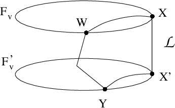
Since the property of alternating was defined completely in terms of the geometry of the pants graph, it must be preserved by the automorphism , so the sequence must also be alternating. Say the edge corresponds to an elementary move (say ) for some curves and —so the marked Farey graph is associated to , then (by the alternating property) the edge must correspond to an elementary move , where and are some other curves (so corresponds to . Now, the edge cannot correspond to a move (by the alternating property again), nor can it correspond to any other move , for , since was chosen to be a 2-curve small loop, and in such a loop, all but two of the curves stay fixed. Therefore, the edge corresponds to a move , and so the marked Farey graph corresponds to , just like .
Illegal Moves. Suppose and differ by the move . There is one illegal move which we will rule out now—the case when and lie on a , and , , and are all non-separating on the . The reason we need to rule this out is that this type of move does not appear in the almost-alternating hexagon (or any of the other small loops previously discussed), and this makes it difficult to find the loop in this case. We need not concern ourselves with this case, because the pants graph is still connected even when the edges corresponding to these moves are removed. In other words, there is a pants decomposition which differs by a move from both and so that the above illegal move does not occur in passing from to or from to . We now prove this fact:
Since is nonseparating on , its complement in the subsurface is a , with the four “punctures” corresponding to the two punctures from and the two “sides” of . Since and are nonseparating curves on the which differ by an elementary move, they each associate (see Section 2) different punctures with a given side of (in particular, they don’t associate the two punctures of the ). Since any edge in is part of a triangle, there is a vertex (two in fact) in (corresponding to a curve ) connected to both vertices corresponding to and , where associates the two punctures of (i.e. is separating on ), since the pants decompositions corresponding to the three vertices of a triangle of have all three different associations. Choose so that the moves and correspond to the moves and .

Finding the Loop. In order find the loop , there are three cases to consider:
1. and lie on disjoint subsurfaces
2. and lie on a
3. and lie on a
Case 1: Choose to be the alternating square , where , , , and have the same curves (in name) in their corresponding pants decompositions as , , , and (from the topological description of alternating squares).
Case 2: Choose to be the alternating pentagon (for unique ), where , , , , and have the same curves in their corresponding pants decompositions as , , , , and respectively (from the topological description of alternating pentagons).
Case 3: Since we eliminated illegal moves, there are two possibilities for the curves , , and —either (i) and is nonseparating, and is separating, or (ii) is separating, and are nonseparating. By symmetry, the first possibility takes care of the case when is nonseparating, is separating, and is nonseparating.
For the first possibility, choose to be the almost alternating hexagon (for unique and ) where , , , , , and , correspond to , , , , , and , respectively (from the topological characterization of almost alternating hexagons). For the latter case, , , , , , and , should correspond to , , , , , and , respectively.
is an automorphism.
Since the curve complex has the property that every set of mutually connected vertices is the -skeleton of a -simplex in the curve complex, we only need to check that extends to an automorphism of the -skeleton of the curve complex, i.e. that takes vertices connected by edges to vertices connected by edges.
Suppose that and are vertices of the curve complex corresponding to curves and on the surface. We will show that and are connected by an edge in the curve complex if and only if there are marked Farey graphs and corresponding to and , where the Farey graphs share a unique point , which is also the marked point on both Farey graphs. Since the number of intersection points between Farey graphs is preserved under the pants graph automorphism , it follows that edges are preserved under .
Let be any pants decomposition containing and , say . Then let and be the set of all pants decompositions of the form and . Then and have the desired property. This construction is possible if and only if and are part of some pants decomposition, which is equivalent to and being connected by an edge.
is an isomorphism.
We show that is a homomorphism that is injective and surjective.
Homomorphism. We will show that in by showing that for any vertex in . is, by definition, the vertex in corresponding to , where is a marked Farey graph in representing , and , being an element of acts on it in the natural way. On the other hand, is the vertex in corresponding to , and hence is the vertex of corresponding to , where is some Farey graph representing . We can in fact choose to be , and so is , which is the same as .
Injectivity. Suppose is the identity automorphism of the curve complex, and let be a vertex of the pants graph corresponding to the pants decomposition , where are the vertices of the curve complex corresponding to the . We will show that . There is a unique choice of (the Farey graph corresponding to the pants decompostions ) representing the so that the all intersect at the point in the pants graph.
Since must be marked Farey graphs corresponding to , it follows that their common intersection point is . Thus .
Surjectivity: There is a natural map obtained by using the isomorphism of Theorem A. The isomorphism is natural in the sense that if a curve corresponds to a vertex of the curve complex, then the curve represents the vertex for any .
Let , and let be a vertex of the pants graph, where is the set of curves . Then is defined to be the vertex of the pants graph which is the curves . Note that preserves edges in since it is has the same action as a mapping class element.
It remains to show that , where . If is a vertex of the curve complex, then we need to show that , where and are marked Farey graphs in the pants graph corresponding to the vertices and of the curve complex. If corresponds to a curve , then the vertices of are all the pants decompositions of the form for some curves which have trivial intersection with . By definition, the vertices of are all of the pants decompositions of the form , and is the pants decomposition . Since corresponds to the vertex of the curve complex, we are done.
References
- [1] Martin R. Bridson and Karen Vogtmann. Automorphisms of automorphism groups of free groups. J. Algebra, 229(2):785–792, 2000.
- [2] Jeffrey Brock. The weil-petersson metric and volumes of 3-dimensional hyperbolic convex cores. Preprint.
- [3] Ruth Charney and Michael Davis. When is a Coxeter system determined by its Coxeter group? J. London Math. Soc. (2), 61(2):441–461, 2000.
- [4] John Harer. The virtual cohomological dimension of the mapping class group of an orientable surface. Invent. Math., 84(1):157–176, 1986.
- [5] W. J. Harvey. Geometric structure of surface mapping class groups. In Homological group theory (Proc. Sympos., Durham, 1977), pages 255–269. Cambridge Univ. Press, Cambridge, 1979.
- [6] Allen Hatcher and William Thurston. A presentation for the mapping class group of a closed orientable surface. Topology, 19(3):221–237, 1980.
- [7] Nikolai Ivanov. Automorphisms of complexes of curves and of Teichmüller spaces. In Progress in knot theory and related topics, pages 113–120. Hermann, Paris, 1997.
- [8] Nikolai Ivanov. Mapping class groups. In Handbook in Geometric Topology. Elsevier, Amsterdam, 2001.
- [9] Mustafa Korkmaz. Automorphisms of complexes of curves on punctured spheres and on punctured tori. Topology Appl., 95(2):85–111, 1999.
- [10] Feng Luo. Automorphisms of the complex of curves. Topology, 39(2):283–298, 2000.
- [11] Howard Masur and Yair Minsky. Geometry of the complex of curves. I. Hyperbolicity. Invent. Math., 138(1):103–149, 1999.
- [12] Howard Masur and Mike Wolf. Weil-petersson isometries. Preprint.
- [13] Yair Minsky. A geometric approach to the complex of curves on a surface. In Topology and Teichmüller spaces (Katinkulta, 1995), pages 149–158. World Sci. Publishing, River Edge, NJ, 1996.
Dan Margalit
Dept. of Mathematics, University of Chicago
5734 University Ave.
Chicago, Il 60637
E-mail: juggler@math.uchicago.edu