跳到论文正文
W Papers独立论文阅读器 arXiv:math/0112196 论文正文 计算阅读时间 · 0%
引用这篇论文根据当前论文元数据生成,正式投稿前建议核对。


License: Assumed arXiv.org perpetual non-exclusive license
arXiv:math/0112196v1 [math.NT] 19 Dec 2001

The Highest-Lowest Zero and other Applications of Positivity

Stephen D. Miller Thanks: The author was supported by an NSF Postdoctoral Fellowship during this work. Affiliation: Department of Mathematics , Yale University , P.O. Box 208283, New Haven, CT 06520-8283
May 16, 1999
Abstract

The first nontrivial zeroes of the Riemann ζ\zeta function are ≈12±14.13472​i\approx\frac{1}{2}\pm 14.13472i. We investigate the question of whether or not any other L-function has a higher lowest zero. To do so we try to quantify the notion that the L-function of a “small” automorphic representation (i.e. one with small level and archimedean type) does not have small zeroes, and vice-versa. We prove that many types of automorphic L-functions have a lower first zero than ζ\zeta’s (see Theorems 1.1 and 1.2). This is done using Weil’s explicit formula with carefully-chosen test functions. When this method does not immediately show L-functions of a certain type have low zeroes, we then attempt to turn the tables and show no L-functions of that type exist. Thus the argument is a combination of proving low zeroes exist and that certain cusp forms do not. Consequently we are able to prove vanishing theorems and improve upon existing bounds on the Laplace spectrum on L2​(S​Ln​(ℤ)\S​Ln​(ℝ)/S​On​(ℝ))L^{2}(SL_{{n}}({\mathbb{Z}})\backslash SL_{{n}}({\mathbb{R}})/SO_{{n}}({\mathbb{R}})). These in turn can be used to show that S​L68​(ℤ)\S​L68​(ℝ)/S​O68​(ℝ)SL_{{68}}({\mathbb{Z}})\backslash SL_{{68}}({\mathbb{R}})/SO_{{68}}({\mathbb{R}}) has a discrete, non-constant, non-cuspidal eigenvalue outside the range of the continuous spectrum on L2​(S​L68​(ℝ)/S​O68​(ℝ))L^{2}(SL_{68}({\mathbb{R}})/SO_{68}({\mathbb{R}})), but that this never happens for S​Ln​(ℤ)\S​Ln​(ℝ)/S​On​(ℝ)SL_{{n}}({\mathbb{Z}})\backslash SL_{{n}}({\mathbb{R}})/SO_{{n}}({\mathbb{R}}) in lower rank. Another application is to cuspidal cohomology: we show there are no cuspidal harmonic forms on S​Ln​(ℤ)\S​Ln​(ℝ)/S​On​(ℝ)SL_{{n}}({\mathbb{Z}})\backslash SL_{{n}}({\mathbb{R}})/SO_{{n}}({\mathbb{R}}) for n<27n<27.

1 Introduction

The Riemann ζ\zeta function’s first critical zeroes are surprisingly large: about 12±14.13472​i\frac{1}{2}\pm 14.13472i. Our main interest in this paper is the following question:

Does any other automorphic L-function have a larger first zero?

This question was raised by Odlyzko ([O]), who proved that the Dedekind zeta function of any number field has a zero whose imaginary part is less than 14. Odlyzko also proved related conditional results for Artin L-functions.

Every automorphic L-function conjecturally factors into products of standard L-functions of cusp forms on G​LnGL_{n} over the rationals, and we shall be content to discuss these.11 1 Nevertheless our arguments work under various wider assumptions, as they are mostly sensitive to the analytic properties of the L-function. In fact, by twisting a cuspidal automorphic representation of G​Ln/ℚGL_{n}/{\mathbb{Q}} by a power of the determinant, it is possible to shift the zeroes any amount vertically, so we restrict ourselves to studying cuspidal automorphic representations π=⊗p≤∞πp\pi_{=}\otimes_{p\leq\infty}\pi_{p} of G​Ln/ℚGL_{n}/{\mathbb{Q}} whose central character is normalized to be trivial. In most examples coming from number theory the archimedean type π∞\pi_{\infty} is real, i.e. the gamma factors multiplying L⁡(s,π)L(s,\pi) have real shifts. Our first result answers the question for such cusp forms:

Theorem 1.1.

Let π\pi be a cuspidal automorphic representation of G​LnGL_{n} over ℚ\mathbb{Q} with a real archimedean type and a trivial central character. Then L⁡(s,π)L(s,\pi) has a low zero which either (i) is on the critical axis between 12±14.13472​i\frac{1}{2}\pm 14.13472i or (ii) violates the generalized Riemann hypothesis (GRH) in an effective range.

When we speak of a zero violating GRH “in an effective range,” we mean that should conclusion (i) fail, then one could theoretically find an effective constant T>0T>0 such that the box (12,1)×[−T,T]​i(\frac{1}{2},1)\times[-T,T]i contains a zero. For brevity we will use the following terminology:

Definition: An L-function has a low zero if it either vanishes on the critical axis between 12±14.13472​i\frac{1}{2}\pm 14.13472i, or violates GRH in an effectively-bounded range (see Section 2.3).

We will use this definition to state unconditional results, but not much is actually gained philosophically or numerically in this problem by assuming GRH.

The L-functions in Theorem 1.1 include those of Dirichlet characters, rational elliptic curves, and conjecturally all rational abelian varieties. Of course they are also expected to include all Artin L-functions, for example L-functions of Galois representations. We have been unable to squeeze our technique to answer Odlyzko’s question in full generality, but can prove many cases. For example:

Theorem 1.2.

Let π\pi be a cuspidal automorphic representation of G​L2GL_{2} over ℚ\mathbb{Q} with a trivial central character. Then L⁡(s,π)L(s,\pi) has a low zero (which is on the critical axis between 12±14.13472​i\frac{1}{2}\pm 14.13472i or else violates GRH in an effective range).

This includes modular form and Maass form L-functions.

Other results can be proven about low zeroes. For example, every L-function which is related to itself by an odd functional equation automatically vanishes at s=1/2s=1/2. For a fixed degree nn, most cuspidal automorphic representations of G​LnGL_{n} over ℚ\mathbb{Q} with a trivial central character have low zeroes. In fact, the possible exceptions all lie in a bounded subset of the unitary dual and have bounded level. This subset tends to be devoid of cusp forms, which is why our method is successful. Thus Odlyzko’s question is related to vanishing theorems about automorphic forms.

Our technique uses Weil’s explicit formula relating the coefficients and zeroes of automorphic L-functions. It is a variation on the Stark-Odlyzko positivity technique, as formulated by Serre, Poitou, Mestre, and others – see [O] for a survey. In particular, one can compute an exact formula for sum of certain test functions over the critical zeroes. If we use a test function which is positive only in a certain range, then finding this sum is positive ensures a zero in that range. On the other hand, if this sum is negative, then we can often construct another test function which is positive in the critical strip, yet whose sum over the zeroes is negative. This contradiction shows that the L-function actually could not have existed to begin with. Our main difficulty is that it is often very difficult to construct this second test function given the failure of the first.

The latter contradiction, of positive terms yielding a negative sum, can be used to prove vanishing theorems about automorphic forms, since they cannot exist when their L-functions do not. Independent of our interest in low zeroes, this leads to applications in group cohomology and spectral theory.

Other applications

One of the consequences of the Ramanujan-Selberg temperedness conjecture is that the discrete cuspidal spectrum of the laplacian Δ\Delta on
L2​(S​Ln​(ℤ)\S​Ln​(ℝ)/S​On​(ℝ))L^{2}(SL_{{n}}({\mathbb{Z}})\backslash SL_{{n}}({\mathbb{R}})/SO_{{n}}({\mathbb{R}})) is contained in the continuous spectrum of Δ\Delta on L2​(S​Ln​(ℝ)/S​On​(ℝ))L^{2}(SL_{n}({\mathbb{R}})/SO_{n}({\mathbb{R}})). (We always normalize Δ\Delta so that this continuous spectrum is the interval [n3−n24,∞)[\frac{n^{3}-n}{24},\infty).) This consequence should be true more generally for congruence covers of S​Ln​(ℤ)\S​Ln​(ℝ)/S​On​(ℝ)SL_{{n}}({\mathbb{Z}})\backslash SL_{{n}}({\mathbb{R}})/SO_{{n}}({\mathbb{R}}), but in this particular case slightly more was proven in [M]:

Theorem 1.3.

([M]): There exists a constant c>0c>0 such that the Laplace eigenvalue of every cusp form ϕ\phi on S​Ln​(ℤ)\S​Ln​(ℝ)/S​On​(ℝ)SL_{{n}}({\mathbb{Z}})\backslash SL_{{n}}({\mathbb{R}})/SO_{{n}}({\mathbb{R}}) satisfies

λ⁡(ϕ)>λ1​(S​Ln​(ℝ)/S​On​(ℝ))+c​n.\lambda(\phi)>\lambda_{1}(SL_{n}({\mathbb{R}})/SO_{n}({\mathbb{R}}))+cn.

Our new result is superior for small nn:

Theorem 1.4.

Let ϕ\phi be a cuspidal eigenfunction of the non-euclidean laplacian Δ\Delta on S​Ln​(ℤ)\S​Ln​(ℝ)/S​On​(ℝ)SL_{n}({\mathbb{Z}})\backslash SL_{n}({\mathbb{R}})/SO_{n}({\mathbb{R}}). Then ϕ\phi’s Laplace eigenvalue satisfies

λ⁡(ϕ)>n3−4​n24+25.92​(1+1n−1).\lambda(\phi)>\frac{n^{3}-4n}{24}+25.92\left(1+\frac{1}{n-1}\right). (1)

It can be applied to answer a question of Alexander Lubotzky: when does the eigenvalue of a noncuspidal, square-integrable eigenfunction of the laplacian on S​Ln​(ℤ)\S​Ln​(ℝ)/S​On​(ℝ)SL_{n}({\mathbb{Z}})\backslash SL_{n}({\mathbb{R}})/SO_{n}({\mathbb{R}}) lie outside [n3−n24,∞)[\frac{n^{3}-n}{24},\infty)?

Theorem 1.5.

If  n≤67n\leq 67, any non-constant eigenfunction of Δ\Delta in
L2​(S​Ln​(ℤ)\S​Ln​(ℝ)/S​On​(ℝ))L^{2}(SL_{{n}}({\mathbb{Z}})\backslash SL_{{n}}({\mathbb{R}})/SO_{{n}}({\mathbb{R}})) has Laplace eigenvalue greater than n3−n24\frac{n^{3}-n}{24}, but the first Laplace eigenvalue of S​L68​(ℤ)\S​L68​(ℝ)/S​O68​(ℝ)SL_{68}({\mathbb{Z}})\backslash SL_{68}({\mathbb{R}})/SO_{68}({\mathbb{R}}) is in fact approximately

12906.6<683−6824=13098.5.12906.6<\frac{68^{3}-68}{24}=13098.5.

Finally, we can apply our technique to cuspidal cohomology and extend a result in [M], where it was shown that S​Ln​(ℤ)\S​Ln​(ℝ)/S​On​(ℝ)SL_{n}({\mathbb{Z}})\backslash SL_{n}({\mathbb{R}})/SO_{n}({\mathbb{R}}) has no harmonic cuspidal automorphic forms for n<23n<23:

Theorem 1.6.

The constant-coefficients cuspidal cohomology of S​Ln​(ℤ)SL_{n}({\mathbb{Z}})

Hc​u​s​p⋅​(S​Ln​(ℤ),ℂ)=0H_{cusp}^{\cdot}(SL_{n}({\mathbb{Z}});{\mathbb{C}})=0

vanishes for 1<n<27.1<n<27.

The technique used to prove this theorem is related to the one in [M]. Fermigier [F] had a similar, but weaker, result using positivity with a different L-function. Here we combine both methods to go further.

Acknowledgements: We wish to thank Don Blasius, William Duke, Benedict Gross, Alexander Lubotzky, Andrew Odlyzko, Ilya Piatetski-Shapiro, Vladimir Rokhlin, Peter Sarnak, Jean-Pierre Serre, Gunther Steil, Andrew Wiles, and Gregg Zuckerman for their discussions. Our point of view on L-functions was influenced by the discussion in [RS]. Support was provided by National Science Foundation Graduate and Postdoctoral Fellowships and a Yale Hellmann fellowship during stays at Princeton University, Yale University, and the University of California at San Diego. All numerical computations were made with Mathematica v.3 on an Intel Pentium II 300 MHz system running Windows NT 4.0 and Slackware Linux 2.0.30.

2 L-functions and positivity

By conjectures of Langlands the most general automorphic L-function is a product of standard L-functions of cuspidal automorphic representations π=⊗p≤∞πp\pi=\otimes_{p\leq\infty}\pi_{p} on G​LmGL_{m} over the rational adeles 𝔸ℚ\mathbb{A}_{\mathbb{Q}}. These “primitive” L-functions are degree mm Euler products

L⁡(s,π)=∏p​ prime∏j=1m(1−αp,j​p−s)−1,αp,j∈ℂL(s,\pi)=\prod_{p\mbox{ prime}}\ \prod_{j=1}^{m}(1-\alpha_{p,j}p^{-s})^{-1}~,~\alpha_{p,j}\in\mathbb{C}

and have completions

Λ⁡(s,π)=∏j=1mπ(−s+ηj)/2​Γ​(s+ηj2)​L​(s,π),ηj∈ℂ\Lambda(s,\pi)=\prod_{j=1}^{m}\pi^{(-s+\eta_{j})/2}\Gamma\left(\frac{s+\eta_{j}}{2}\right)L(s,\pi)~,~\eta_{j}\in{\mathbb{C}}

which are entire unless m=1m=1 and L⁡(s)=ζ⁡(s)L(s)=\zeta(s). We have used the duplication property of the gamma function in writing the gamma factors in this way. The conductor is DD, and for πp\pi_{p} unramified, the αp,j\alpha_{p,j} are Hecke eigenvalue parameters and the ηj\eta_{j} are related to the archimedean parameters of π∞\pi_{\infty}. With this normalization Λ⁡(s,π)\Lambda(s,\pi) has the functional equation

Λ⁡(s,π)=τπ​D−s​Λ​(1−s,π~),τπ∈ℂ,|τπ|=D,D>0,\Lambda(s,\pi)=\tau_{\pi}D^{-s}\Lambda(1-s,\tilde{\pi})~,~\tau_{\pi}\in{\mathbb{C}}~,~|\tau_{\pi}|=\sqrt{D}~,~D>0,

where π~\tilde{\pi} is the contragredient representation to π\pi. The Jacquet-Shalika ([JS]) bounds imply that

Re ​ηj>−12.\mbox{Re~}{\eta_{j}}>-\frac{1}{2}. (2)

2.1 Weil’s formula

The explicit formula of André Weil equates a sum over the zeroes of an L-function with a sum over its coefficients and gamma factors:

∑Λ⁡(12+i​γ,π)=0h⁡(γ)=2​Re ​{∑j=1ml⁡(ηj)−∑n=1∞cnn​g​(log⁡n)}+g⁡(0)​log⁡D,\sum_{\Lambda(\frac{1}{2}+i\gamma,\pi)=0}h(\gamma)=2\mbox{Re~}\left\{\sum_{j=1}^{m}l(\eta_{j})-\sum_{n=1}^{\infty}\frac{c_{n}}{\sqrt{n}}g(\log n)\right\}+g(0)\log{D}, (3)

where gg is an even, differentiable real function,

g^​(r)=h⁡(r)=∫ℝg⁡(x)​ei​r​x​𝑑x,\hat{g}(r)=h(r)=\int_{{\mathbb{R}}}g(x)e^{irx}dx,
Γℝ(s)=π−s/2Γ(s/2),\Gamma_{{\mathbb{R}}}(s)=\pi^{-s/2}\Gamma(s/2),

and

l⁡(η)=12​π​∫ℝh⁡(r)​Γℝ′Γℝ​(12+η+i​r)​𝑑rl(\eta)=\frac{1}{2\pi}\int_{{\mathbb{R}}}h(r)\frac{\Gamma_{{\mathbb{R}}}^{\prime}}{\Gamma_{{\mathbb{R}}}}\left(\frac{1}{2}+\eta+ir\right)dr
=12​π​∫ℝh⁡(r)​(−log⁡π2)​𝑑r+12​π​∫ℝh⁡(r)​Γ′2​Γ​(14+η2+i​r2)​𝑑r=\frac{1}{2\pi}\int_{{\mathbb{R}}}h(r)\left(\frac{-\log\pi}{2}\right)dr+\frac{1}{2\pi}\int_{{\mathbb{R}}}h(r)\frac{\Gamma^{\prime}}{2\Gamma}\left(\frac{1}{4}+\frac{\eta}{2}+\frac{ir}{2}\right)dr
=−log⁡π2​g​(0)−12​∫0∞(g⁡(x/2)​e−(1/4+η/2)​x1−e−x−g⁡(0)ex​x)​𝑑x.=-\frac{\log\pi}{2}g(0)-\frac{1}{2}\int_{0}^{\infty}\left(\frac{g(x/2)e^{-(1/4+\eta/2)x}}{1-e^{-x}}-\frac{g(0)}{e^{x}x}\right)dx.

Here we have made use of the fact that L⁡(s,π)L(s,\pi) is entire; for ζ⁡(s)\zeta(s) and Rankin-Selberg L-functions there is a polar term that will be introduced when needed later on. See [RS] for a proof of (3).

If gg is supported in the interval [−log⁡2,log⁡2][-\log 2,\log 2] then the formula can be viewed as giving the value of the sum over the zeroes from the gamma factors:

∑h⁡(γ)=2​Re ​∑j=1ml⁡(ηj)+g⁡(0)​log⁡D.\sum h(\gamma)=2\mbox{Re~}\sum_{j=1}^{m}l(\eta_{j})+g(0)\log D. (4)

The basis of the positivity technique is the observation that if h⁡(γ)≥0h(\gamma)\geq 0 for each zero, then the sum on the right-hand side of (4) must also be positive. This immediately gives a lower bound on the conductor DD, which is the original application of the positivity technique. Fortunately the sum on the right-hand side of (4) is explicitly computable in terms of the ηj\eta_{j}’s and DD; if it is negative then the L-function L⁡(s,π)L(s,\pi) cannot exist and hence neither can the original cusp form π\pi.

Upon assuming GRH, let

⋯≤γ−2≤γ−1≤0≤γ1≤γ2≤⋯\cdots\leq\gamma_{-2}\leq\gamma_{-1}\leq 0\leq\gamma_{1}\leq\gamma_{2}\leq\cdots

be the imaginary parts of the zeroes of L⁡(s,π)L(s,\pi). Let gg and h=g^h=\hat{g} be chosen so that h≥0h\geq 0 on ℝ\mathbb{R} and let c>0c>0 be a cutoff parameter. Then the function hm​(r)=h⁡(r)​(c2−r2)h_{m}(r)=h(r)(c^{2}-r^{2}) is positive exactly when |r|<c|r|<c and is the Fourier transform of gm=c2​g+g′′g_{m}=c^{2}g+g^{\prime\prime}. The support of gmg_{m} is of course also contained in [−log⁡2,log⁡2][-\log 2,\log 2] provided gg is suitably regular. If the sum 2​Re ​∑j=1mlm​(ηj)+gm​(0)​log⁡D2\mbox{Re~}\sum_{j=1}^{m}l_{m}(\eta_{j})+g_{m}(0)\log D in (4) is positive, then γ1<c\gamma_{1}<c or γ−1>−c\gamma_{-1}>-c, i.e. L⁡(s,π)L(s,\pi) has a small zero. To summarize:

2.2 Criteria

Our strategy will then be, for given archimedean parameters ηj\eta_{j} and conductor DD, to find a function gg of support contained in [−log⁡2,log⁡2][-\log 2,\log 2] and for which either

2​Re ​∑j=1ml⁡(ηj)+g⁡(0)​log⁡D<02\mbox{Re~}\sum_{j=1}^{m}l(\eta_{j})+g(0)\log D<0

(which shows the L-function does not exist) or

2​Re ​∑j=1mlm​(ηj)+gm​(0)​log⁡D>02\mbox{Re~}\sum_{j=1}^{m}l_{m}(\eta_{j})+g_{m}(0)\log D>0

(which shows that it must have a low zero or violate GRH in an effective range, as discussed below).

2.3 What low zeroes mean without GRH

Even if we do not assume GRH, we may still conclude from

2​Re ​∑j=1mlm​(ηj)+gm​(0)​log⁡D>02\mbox{Re~}\sum_{j=1}^{m}l_{m}(\eta_{j})+g_{m}(0)\log D>0

that the sum

∑hm​(γ)>0.\sum h_{m}(\gamma)>0.

Thus, there are zeroes ρ=12+i​γ\rho=\frac{1}{2}+i\gamma in the region where hm​(γ)>0h_{m}(\gamma)>0. We can explicitly compute the functions hmh_{m} for our choices of gg and examine where they are positive and negative within the critical strip. Since the density of zeroes increases only logarithmically with their height (with an effective constant), and our functions hm​(z)h_{m}(z) decay polynomially as z→∞z\rightarrow\infty in the critical strip, the zero must be contained in an effectively bounded region of the critical strip.

As an example, Figure 1 is a contour plot of the function h1​mh_{1m} defined at the end of Section 3. The white regions are where Re ​h1​m>0\mbox{Re~}h_{1m}>0, the black where Re ​h1​m<0\mbox{Re~}h_{1m}<0.

Refer to caption
Figure 1: A contour plot of the function Re ​h1​m​(x+i​y)\mbox{Re~}h_{1m}(x+iy). We have colored the positive set white and the negative one black.

Figures 2 and 3 contain plots for the other functions we use.

3 A library of functions

The main functions we use in this paper are

g1,p​(x)=((π⁡(1−|x|p)​cos⁡(π​xp))+sin⁡(π​|x|p)π)/cosh⁡(x/2),g_{1,p}(x)=\left({\frac{\left(\pi\left(1-{\frac{|x|}{p}}\right)\cos({\frac{\pi x}{p}})\right)+\sin({\frac{\pi|x|}{p}})}{\pi}}\right)/\cosh(x/2),
g2,p​(x)=(4​π​(1−|x|p)+2​π​(1−|x|p)​cos⁡(2​π​xp)+3​sin⁡(2​π​|x|p)6​π)/cosh⁡(x/2),g_{2,p}(x)=\left({\frac{4\pi\left(1-{\frac{|x|}{p}}\right)+2\pi\left(1-{\frac{|x|}{p}}\right)\cos({\frac{2\pi x}{p}})+3\sin({\frac{2\pi|x|}{p}})}{6\pi}}\right)/\cosh(x/2),

and

g3,p​(x)=(54​π​(1−|x|p)​cos⁡(π​xp)+6​π​(1−|x|p)​cos⁡(3​π​xp)+27​sin⁡(π​|x|p)+11​sin⁡(3​π​|x|p)60​π)cosh⁡(x/2).g_{3,p}(x)=\frac{\left({\frac{54\pi\left(1-{\frac{|x|}{p}}\right)\cos({\frac{\pi x}{p}})+6\pi\left(1-{\frac{|x|}{p}}\right)\cos({\frac{3\pi x}{p}})+27\sin({\frac{\pi|x|}{p}})+11\sin({\frac{3\pi|x|}{p}})}{60\pi}}\right)}{\cosh(x/2)}.

We have normalized gj,p​(0)=1g_{j,p}(0)=1 and will often write gj​(x)=gj,log⁡(2)​(x)g_{j}(x)=g_{j,\log(2)}(x). Ignoring the cosh⁡(x/2)\cosh(x/2)’s temporarily, the functions gj,pg_{j,p} are rescalings of the convolutions of (cos⁡(π​x2))j(\cos(\frac{\pi x}{2}))^{j} with itself. Without the cosh⁡(x/2)\cosh(x/2) term they would thus have a positive Fourier transform on the real line, and the cosh⁡(x/2)\cosh(x/2) term spreads the positivity into the critical strip. Were we to assume GRH we would not need it.

Lemma 3.1.

If an even function g⁡(x)g(x)’s Fourier transform is positive on the real line, then the Fourier transform of g⁡(x)/cosh⁡(x/2)g(x)/\cosh(x/2) is positive in the strip −12<Im ​r<12-\frac{1}{2}<\mbox{Im~}r<\frac{1}{2}.

Proof: The Fourier transform of sech​(x)\mbox{sech}(x) is

∫−∞∞2ex+e−x​ei​r​x​𝑑x=π​sech​(π​r/2).\int_{-\infty}^{\infty}\frac{2}{e^{x}+e^{-x}}e^{irx}dx~~~=~~~\pi\mbox{sech}(\pi r/2).

This has positive real part for −12<Im ​r<12-\frac{1}{2}<\mbox{Im~}r<\frac{1}{2} and the Fourier transform converts multiplication into convolution, so the smeared g⋅sech^\widehat{g\cdot\mbox{sech}} remains positive in this strip. □\Box

We defined modified functions

gm=c2​g​(x)+g′′​(x)c2​g​(0)+g′′​(0),g_{m}=\frac{c^{2}g(x)+g^{\prime\prime}(x)}{c^{2}g(0)+g^{\prime\prime}(0)},

which also have gm​(0)=1g_{m}(0)=1. (Of course we multiplicatively normalize g⁡(0)=gm​(0)=1g(0)=g_{m}(0)=1 to compare the explicit formulas from various test functions.) These are used for showing the presence of low zeroes, and since we do not assume GRH for this, we will actually use g=g1,p​(x)​cosh⁡(x/2),g2,p​(x)​cosh⁡(x/2),g=g_{1,p}(x)\cosh(x/2),g_{2,p}(x)\cosh(x/2), or g3,p​(x)​cosh⁡(x/2)g_{3,p}(x)\cosh(x/2). Thus

g1​m,p,c​(x)=π2​(−1+|x|p)​cos⁡(π​xp)p2+π​sin⁡(π​|x|p)p2−c2​(−(π⁡(1−|x|p)​cos⁡(π​xp))−sin⁡(π​|x|p))πc2−π2p2g_{1m,p,c}(x)={\frac{{\frac{{{\pi}^{2}}\left(-1+{\frac{|x|}{p}}\right)\cos({\frac{\pi x}{p}})}{{p^{2}}}}+{\frac{\pi\sin({\frac{\pi|x|}{p}})}{{p^{2}}}}-{\frac{{c^{2}}\left(-\left(\pi\left(1-{\frac{|x|}{p}}\right)\cos({\frac{\pi x}{p}})\right)-\sin({\frac{\pi|x|}{p}})\right)}{\pi}}}{{c^{2}}-{\frac{{{\pi}^{2}}}{{p^{2}}}}}}
g2​m,p,c​(x)=c2​(4​π​(1−|x|p)+2​π​(1−xp)​cos⁡(2​π​xp)+3​sin⁡(2​π​|x|p))6​π−8​π3​(1−xp)​cos⁡(2​π​xp)p2+4​π2​sin⁡(2​π​|x|p)p26​πc2−4​π23​p2g_{2m,p,c}(x)={\frac{{\frac{{c^{2}}\left(4\pi\left(1-{\frac{|x|}{p}}\right)+2\pi\left(1-{\frac{x}{p}}\right)\cos({\frac{2\pi x}{p}})+3\sin({\frac{2\pi|x|}{p}})\right)}{6\pi}}-{\frac{{\frac{8{{\pi}^{3}}\left(1-{\frac{x}{p}}\right)\cos({\frac{2\pi x}{p}})}{{p^{2}}}}+{\frac{4{{\pi}^{2}}\sin({\frac{2\pi|x|}{p}})}{{p^{2}}}}}{6\pi}}}{{c^{2}}-{\frac{4{{\pi}^{2}}}{3{p^{2}}}}}}

and

g3​m,p,c​(x)=g_{3m,p,c}(x)=~~~~~~~~~~~~~~~~~~~~~~~~~~~~~~~~~~~~~~~~~~~~~~~~~~~~~~~~~~~~~~~~~~~~~~~~~
c2​(54​π​(1−|x|p)​cos⁡(π​xp)+6​π​(1−|x|p)​cos⁡(3​π​xp)+27​sin⁡(π​|x|p)+11​sin⁡(3​π​|x|p))60​π​(c2−9​π25​p2)+\displaystyle\frac{c^{2}\left(54\pi\left(1-{\frac{|x|}{p}}\right)\cos({\frac{\pi x}{p}})+6\pi\left(1-{\frac{|x|}{p}}\right)\cos({\frac{3\pi x}{p}})+27\sin({\frac{\pi|x|}{p}})+11\sin({\frac{3\pi|x|}{p}})\right)}{60\pi\left(c^{2}-\frac{9\pi^{2}}{5p^{2}}\right)}~~+
54​π3​(−1+|x|p)​cos⁡(π​xp)+54​π3​(−1+|x|p)​cos⁡(3​π​xp)+81​π2​sin⁡(π​|x|p)−63​π2​sin⁡(3​π​|x|p)60​π​p2​(c2−9​π25​p2).\displaystyle\frac{54\pi^{3}\left(-1+{\frac{|x|}{p}}\right)\cos({\frac{\pi x}{p}})+54{{\pi}^{3}}\left(-1+{\frac{|x|}{p}}\right)\cos({\frac{3\pi x}{p}})+81{{\pi}^{2}}\sin({\frac{\pi|x|}{p}})-63{{\pi}^{2}}\sin({\frac{3\pi|x|}{p}})}{60\pi p^{2}\left({c^{2}}-{\frac{9{{\pi}^{2}}}{5{p^{2}}}}\right)}~.

Since we are interested in finding zeroes in the range from 12±14.13472​i\frac{1}{2}\pm 14.13472i, we will now take c=14.13472c=14.13472 and write

g1​m​(x)=g1​m,log⁡(2),14.13472​(x),g_{1m}(x)=g_{1m,\log(2),14.13472}(x),
g2​m​(x)=g2​m,log⁡(2),14.13472​(x),g_{2m}(x)=g_{2m,\log(2),14.13472}(x),

and

g3​m​(x)=g3​m,log⁡(2),14.13472​(x).g_{3m}(x)=g_{3m,\log(2),14.13472}(x).

The Fourier transforms of these functions are

h1​m​(r)=−8p3π2(c2−x2)cos(p​x2)2(−c2​p2+π2)​(π−p​x)2​(π+p​x)2,h_{1m}(r)={\frac{-8{p^{3}}{{\pi}^{2}}\left({c^{2}}-{x^{2}}\right){{\cos({\frac{px}{2}})}^{2}}}{\left(-{c^{2}}{p^{2}}+{{\pi}^{2}}\right){{\left(\pi-px\right)}^{2}}{{\left(\pi+px\right)}^{2}}}},
h2​m​(r)=128pπ4(c2−x2)sin(p​x2)2(3​c2​p2−4​π2)​(−4​π2​x+p2​x3)2,h_{2m}(r)={\frac{128p{{\pi}^{4}}\left({c^{2}}-{x^{2}}\right){{\sin({\frac{px}{2}})}^{2}}}{\left(3{c^{2}}{p^{2}}-4{{\pi}^{2}}\right){{\left(-4{{\pi}^{2}}x+{p^{2}}{x^{3}}\right)}^{2}}}},

and

h3​m​(r)=2304p3π6(c2−x2)cos(p​x2)2(5​c2​p2−9​π2)​(9​π4−10​p2​π2​x2+p4​x4)2.h_{3m}(r)={\frac{2304{p^{3}}{{\pi}^{6}}\left({c^{2}}-{x^{2}}\right){{\cos({\frac{px}{2}})}^{2}}}{\left(5{c^{2}}{p^{2}}-9{{\pi}^{2}}\right){{\left(9{{\pi}^{4}}-10{p^{2}}{{\pi}^{2}}{x^{2}}+{p^{4}}{x^{4}}\right)}^{2}}}}.

We show the contour plots of the functions h2​mh_{2m} and h3​mh_{3m} in Figures 2 and 3, the plot of h1​mh_{1m} having been presented above in Figure 1.

Refer to caption
Figure 2: A contour plot of the function Re ​h2​m​(x+i​y)\mbox{Re~}h_{2m}(x+iy). We have colored the positive set white and the negative one black.
Refer to caption
Figure 3: A contour plot of the function Re ​h3​m​(x+i​y)\mbox{Re~}h_{3m}(x+iy). We have colored the positive set white and the negative set black.

4 The highest lowest zero for π∞\pi_{\infty} real

We restate

Theorem 4.1 (=1.1).

Let π=⊗p≤∞πp\pi=\otimes_{p\leq\infty}\pi_{p} be a cuspidal automorphic representation of G​LnGL_{n} over ℚ\mathbb{Q} with a trivial central character and whose archimedean type π∞\pi_{\infty} is real. Then L⁡(s,π)L(s,\pi) has a low zero.

First we will note that for a fixed degree mm, L-functions with large ηj\eta_{j}’s or large conductor DD must have low zeroes. This is because Stirling’s formula implies that

l⁡(η)=12​π​∫ℝh⁡(r)​Γℝ′Γℝ​(12+η+i​r)​𝑑rl(\eta)=\frac{1}{2\pi}\int_{{\mathbb{R}}}h(r)\frac{\Gamma_{{\mathbb{R}}}^{\prime}}{\Gamma_{{\mathbb{R}}}}\left(\frac{1}{2}+\eta+ir\right)dr

has a positive real part for η\eta large. Thus, the lowest zero is only an issue for “small” archimedean parameters ηj\eta_{j} and small conductor – partly because l⁡(η)l(\eta) is bounded from below in Re ​η>−12\mbox{Re~}\eta>-\frac{1}{2} (which we may assume by (2)).

We will present two different proofs of Theorem 1.1.

Picture Proof of Theorem 1.1: Figures 4, 5, and 6 indicate that l1​(η)<l3​m​(η)l_{1}(\eta)<l_{3m}(\eta) for η≥−12\eta\geq-\frac{1}{2}, so the theorem follows from Criteria 2.2.

Refer to caption
Figure 4: The functions l⁡(η)l(\eta) and l3​m​(η)l_{3m}(\eta).
Refer to caption
Figure 5: The difference between l⁡(η)l(\eta) and l3​m​(η)l_{3m}(\eta)
Refer to caption
Figure 6: The difference between l⁡(η)l(\eta) and l3​m​(η)l_{3m}(\eta), magnified.

□\Box

Less-Pictorial Proof of Theorem 1.1: This proof also relies on numerical computation, but demonstrates how a proof can be made even if the function ll is not strictly less than the modified lml_{m}. It uses l2​ml_{2m} instead of l3​ml_{3m}.

We noted before in Criteria 2.2 that if

2​∑j=1ml2​m​(ηj)+log⁡D≥02\sum_{j=1}^{m}l_{2m}(\eta_{j})+\log D\geq 0

then there is a indeed a low zero, while if

2​∑j=1ml1​(ηj)+log⁡D≤0,2\sum_{j=1}^{m}l_{1}(\eta_{j})+\log D\leq 0,

the L-function actually cannot exist to begin with. Thus we are reduced to dismissing the situation where

∑j=1ml2​m​(ηj)<0\sum_{j=1}^{m}l_{2m}(\eta_{j})<0

and

∑j=1m[l1​(ηj)−l2​m​(ηj)]>0\sum_{j=1}^{m}\left[l_{1}(\eta_{j})-l_{2m}(\eta_{j})\right]>0

hold simultaneously. Partition the ηj∈(−12,∞)\eta_{j}\in(-\frac{1}{2},\infty) into 3 sets:

N={ηj∣l2​m(ηj)≤0,l1(ηj)−l2​m(ηj)≤0}=(−12,5.4471⋯],N=\left\{\eta_{j}\mid l_{2m}(\eta_{j})\leq 0,l_{1}(\eta_{j})-l_{2m}(\eta_{j})\leq 0\right\}~~=~~(-\frac{1}{2}~,~5.4471\cdots],
S={ηj∣l2​m(ηj)>0,l1(ηj)−l2​m(ηj)≤0}=(5.4472⋯,8.6553⋯],S=\left\{\eta_{j}\mid l_{2m}(\eta_{j})>0,l_{1}(\eta_{j})-l_{2m}(\eta_{j})\leq 0\right\}~~=~~(5.4472\cdots~,~8.6553\cdots],

and

P={ηj∣l2​m(ηj)>0,l1(ηj)−l2​m(ηj)>0}=(8.6553⋯,∞).P=\left\{\eta_{j}\mid l_{2m}(\eta_{j})>0,l_{1}(\eta_{j})-l_{2m}(\eta_{j})>0\right\}~~=~~(8.6553\cdots~,~\infty).

Of course if

∑j=1ml2​m​(ηj)<0,\sum_{j=1}^{m}l_{2m}(\eta_{j})<0,

then also

∑ηj∈N∪Pl2​m​(ηj)<0,\sum_{\eta_{j}\in N\cup P}l_{2m}(\eta_{j})<0,

and if

∑j=1m[l1​(ηj)−l2​m​(ηj)]>0,\sum_{j=1}^{m}\left[l_{1}(\eta_{j})-l_{2m}(\eta_{j})\right]>0,

then

∑ηj∈N∪P[l1​(ηj)−l2​m​(ηj)]>0\sum_{\eta_{j}\in N\cup P}\left[l_{1}(\eta_{j})-l_{2m}(\eta_{j})\right]>0

as well. Thus we need only consider the case where SS is empty.

From computer investigations (see Figure 8) on the functions l1​(η)l_{1}(\eta) and l2​m​(η)l_{2m}(\eta) we can determine the following very precise information:

Refer to caption
Figure 7: The difference between l⁡(η)l(\eta) and l2​m​(η)l_{2m}(\eta).
Refer to caption
Figure 8: The graphs of l⁡(η)l(\eta) and l2​m​(η)l_{2m}(\eta).
ηj∈N⟹−.628291≤l1​(ηj)≤0,l1​(ηj)−l2​m​(ηj)≤−.001201\eta_{j}\in N\Longrightarrow-.628291\leq l_{1}(\eta_{j})\leq 0~~~~,~~~~l_{1}(\eta_{j})-l_{2m}(\eta_{j})\leq-.001201

and

ηj∈P⟹l1​(ηj)≥.187484,0≤l1​(ηj)−l2​m​(ηj)≤.0005801.\eta_{j}\in P\Longrightarrow l_{1}(\eta_{j})\geq.187484~~~~~~~,~~~~~~~0\leq l_{1}(\eta_{j})-l_{2m}(\eta_{j})\leq.0005801.

Thus

0>∑j=1ml2​m​(ηj)=∑ηj∈Nl2​m​(ηj)+∑ηj∈Pl2​m​(ηj)0>\sum_{j=1}^{m}l_{2m}(\eta_{j})=\sum_{\eta_{j}\in N}l_{2m}(\eta_{j})+\sum_{\eta_{j}\in P}l_{2m}(\eta_{j})
≥|N​|(−.628291)+|​P|(.187484),\geq|N|(-.628291)+|P|(.187484),

which implies

|N||P|<.187484.628291=.298403.\frac{|N|}{|P|}<\frac{.187484}{.628291}=.298403.

On the other hand

0<∑j=1m[l1​(ηj)−l2​m​(ηj)]=∑ηj∈N[l1​(ηj)−l2​m​(ηj)]+∑ηj∈P[l1​(ηj)−l2​m​(ηj)]0<\sum_{j=1}^{m}\left[l_{1}(\eta_{j})-l_{2m}(\eta_{j})\right]=\sum_{\eta_{j}\in N}\left[l_{1}(\eta_{j})-l_{2m}(\eta_{j})\right]+\sum_{\eta_{j}\in P}\left[l_{1}(\eta_{j})-l_{2m}(\eta_{j})\right]
≤|N​|(−.001201)+|​P|(.005801)\leq|N|(-.001201)+|P|(.005801)

forces

|N||P|>.0005801.001201=.483104,\frac{|N|}{|P|}>\frac{.0005801}{.001201}=.483104,

a contradiction. □\Box

5 Low zeroes for modular form L-functions

In this section we prove that L-functions of cusp forms on G​L2GL_{2} over ℚ\mathbb{Q} have low zeroes:

Theorem 5.1 (=1.2).

Let π\pi be a cuspidal automorphic representation of G​L2GL_{2} over ℚ\mathbb{Q} with a trivial central character. Then L⁡(s,π)L(s,\pi) has a low zero.

Before giving the proof we shall give some background on the hardest case – Maass form L-functions. In particular we will precisely describe their completions, analytic continuations, and functional equations in some important cases.

5.1 Background on Maass forms on Γ0​(p)\ℍ\Gamma_{0}(p)\backslash\mathbb{H}

It is known that if D=pD=p is a prime and π\pi is a cuspidal automorphic representation not corresponding to a holomorphic modular form, then π\pi instead corresponds to a Maass form ϕ\phi on Γ0​(p)\ℍ\Gamma_{0}(p)\backslash\mathbb{H}. The Laplace operator Δ\Delta, the Hecke operators Tn,n≥0T_{n},n\geq 0, as well as the involutions

(T−1​f)​(x+i​y)=f⁡(−x+i​y)(T_{-1}f)(x+iy)=f(-x+iy)
(Wp​f)​(x+i​y)=f⁡(−1p⁡(x+i​y))(W_{p}f)(x+iy)=f\left(\frac{-1}{p(x+iy)}\right)

all commute. Thus, after diagonalizing, we may take a basis of Maass cusp forms on Γ0​(p)\ℍ\Gamma_{0}(p)\backslash\mathbb{H} which are joint eigenfunctions of Δ,Tn,T−1,\Delta,T_{n},T_{-1}, and WpW_{p}. Writing

Δ​ϕ=λ​ϕ,λ=14−ν2,\Delta\phi=\lambda\phi~~,~~\lambda=\frac{1}{4}-\nu^{2},

ϕ\phi has the Fourier expansion

ϕ⁡(x+i​y)=∑n∈ℤcn​y​Kν​(2​π​|n|​y)​e2​π​i​n​x,\phi(x+iy)=\sum_{n\in{\mathbb{Z}}}c_{n}\sqrt{y}K_{\nu}(2\pi|n|y)e^{2\pi inx},

where

Kν=K−ν=12∫0∞e−y(t+t−1)/2tνd​ttK_{\nu}=K_{-\nu}=\frac{1}{2}\int_{0}^{\infty}e^{-y(t+t^{-1})/2}t^{\nu}\frac{dt}{t}

is the KK-Bessel function of order ν\nu. The cuspidality condition forces c0=0c_{0}=0; the involution T−1T_{-1} interchanges cnc_{n} and c−nc_{-n}.

There are four symmetry classes of Maass forms under the action of the involutions T−1T_{-1} and WpW_{p}. The standard argument of Hecke and Maass to prove that the L-functions of cusp forms are entire also describes the functional equations of L-functions of Maass forms having various symmetries.

Proposition 5.2.

Suppose ϕ\phi is a Maass form on Γ0​(p)\ℍ\Gamma_{0}(p)\backslash\mathbb{H} with

T−1​ϕ=(−1)τ​ϕT_{-1}\phi=(-1)^{\tau}\phi

and

Wp​ϕ=(−1)ω​ϕ,τ,ω=0​ or ​1.W_{p}\phi=(-1)^{\omega}\phi~~,~~\tau,\omega=0\mbox{ or }1.

Multiplicatively normalize the coefficients of ϕ\phi so that a1=1a_{1}=1 and

ϕ⁡(x+i​y)={∑n=1∞an​y​Kν​(2​π​n​y)​cos⁡(2​π​n​x),τ=0∑n=1∞an​y​Kν​(2​π​n​y)​sin⁡(2​π​n​x),τ=1.\phi(x+iy)=\left\{\begin{array}[]{ll}\sum_{n=1}^{\infty}a_{n}\sqrt{y}K_{\nu}(2\pi ny)\cos(2\pi nx),&\tau=0\\ \sum_{n=1}^{\infty}a_{n}\sqrt{y}K_{\nu}(2\pi ny)\sin(2\pi nx),&\tau=1.\\ \end{array}\right.

Then

Λ⁡(s,ϕ)=Γℝ​(s+τ+ν)​Γℝ​(s+τ−ν)​∑n=1∞anns\Lambda(s,\phi)=\Gamma_{{\mathbb{R}}}(s+\tau+\nu)\Gamma_{{\mathbb{R}}}(s+\tau-\nu)\sum_{n=1}^{\infty}\frac{a_{n}}{n^{s}}

satisfies the functional equation

Λ⁡(s,ϕ)=(−1)τ+ω​p1/2−s​Λ​(1−s,ϕ).\Lambda(s,\phi)=(-1)^{\tau+\omega}p^{1/2-s}\Lambda(1-s,\phi). (5)

Proof: First consider the case τ=0\tau=0. Then

∫0∞ϕ⁡(i​y)​ys−1/2​d​yy=∑n=1∞an​∫0∞Kν​(2​π​n​y)​ys​d​yy\int_{0}^{\infty}\phi(iy)y^{s-1/2}\frac{dy}{y}=\ \sum_{n=1}^{\infty}a_{n}\int_{0}^{\infty}K_{\nu}(2\pi ny)y^{s}\frac{dy}{y}
=∑n=1∞an​(2​π​n)−s​[∫0∞Kν​(y)​ys​d​yy]=\sum_{n=1}^{\infty}a_{n}(2\pi n)^{-s}\left[\int_{0}^{\infty}K_{\nu}(y)y^{s}\frac{dy}{y}\right]
=∑n=1∞an​(2​π​n)−s​[2s−2​Γ​(s+ν2)​Γ​(s−ν2)]=\sum_{n=1}^{\infty}a_{n}(2\pi n)^{-s}\left[2^{s-2}\Gamma(\frac{s+\nu}{2})\Gamma(\frac{s-\nu}{2})\right]
=14​Λ​(s,ϕ).=\frac{1}{4}\Lambda(s,\phi).

The transformation property

ϕ⁡(i​y)=(−1)ω​ϕ​(ip​y)\phi(iy)=(-1)^{\omega}\phi(\frac{i}{py})

gives

Λ⁡(s,ϕ)=4​∫0∞ϕ⁡(i​y)​ys−1/2​d​yy=4​(−1)ω​∫0∞ϕ⁡(ip​y)​ys−1/2​d​yy\Lambda(s,\phi)=4\int_{0}^{\infty}\phi(iy)y^{s-1/2}\frac{dy}{y}=4(-1)^{\omega}\int_{0}^{\infty}\phi(\frac{i}{py})y^{s-1/2}\frac{dy}{y}
=4​(−1)ω​∫0∞ϕ⁡(i​yp)​y1/2−s​d​yy=4(-1)^{\omega}\int_{0}^{\infty}\phi(\frac{iy}{p})y^{1/2-s}\frac{dy}{y}
=4​p1/2−s​(−1)ω​∫0∞ϕ⁡(i​y)​y1/2−s​d​yy=4p^{1/2-s}(-1)^{\omega}\int_{0}^{\infty}\phi(iy)y^{1/2-s}\frac{dy}{y}
=(−1)ω​p1/2−s​Λ​(1−s,ϕ).=(-1)^{\omega}p^{1/2-s}\Lambda(1-s,\phi).

If instead τ=1\tau=1 then actually ϕ⁡(i​y)=0\phi(iy)=0 and we instead consider the derivative

ϕ′​(x+i​y):=dd​x​ϕ​(x+i​y)\phi^{\prime}(x+iy):=\frac{d}{dx}\phi(x+iy)
=∑n=1∞(2​π​n)​an​y​Kν​(2​π​n​y)​cos⁡(2​π​n​x).=\sum_{n=1}^{\infty}(2\pi n)a_{n}\sqrt{y}K_{\nu}(2\pi ny)\cos(2\pi nx).

The action under WpW_{p} now reads

ϕ′​(i​y)=(−1)ω​ϕ′​(ip​y2)​(−1p​y2).\phi^{\prime}(iy)=(-1)^{\omega}\phi^{\prime}(\frac{i}{py^{2}})(\frac{-1}{py^{2}}).

We also have that

∫0∞ϕ′​(i​y)​ys+1/2​d​yy=∑n=1∞(2​π​n)​an​∫0∞Kν​(2​π​n​y)​ys+1​d​yy\int_{0}^{\infty}\phi^{\prime}(iy)y^{s+1/2}\frac{dy}{y}=\sum_{n=1}^{\infty}(2\pi n)a_{n}\int_{0}^{\infty}K_{\nu}(2\pi ny)y^{s+1}\frac{dy}{y}
=∑n=1∞an​(2​π​n)−s​[2s−1​Γ​(s+1+ν2)​Γ​(s+1−ν2)],=\sum_{n=1}^{\infty}a_{n}(2\pi n)^{-s}\left[2^{s-1}\Gamma(\frac{s+1+\nu}{2})\Gamma(\frac{s+1-\nu}{2})\right],

and the functional equation for Λ⁡(s,ϕ)\Lambda(s,\phi) follows as before. □\Box

5.2 Low zeroes for Maass form L-functions

We will first prove Theorem 5.1 for Maass forms through a series of propositions.

Proposition 5.3.

Every Maass form L-function whose conductor satisfies

D≥3,if ​T−1​ϕ=ϕD\geq 3~~,~~\mbox{if }~~T_{-1}\phi=\phi

or

D≥2,if ​T−1​ϕ=−ϕD\geq 2~~,~~\mbox{if }~~T_{-1}\phi=-\phi

has a low zero.

Proof: In these two symmetry classes the gamma factors of Λ⁡(s,ϕ)\Lambda(s,\phi) are either

Γℝ​(s+ν)​Γℝ​(s−ν)\Gamma_{{\mathbb{R}}}(s+\nu)\Gamma_{{\mathbb{R}}}(s-\nu)

or

Γℝ​(s+1+ν)​Γℝ​(s+1−ν),\Gamma_{{\mathbb{R}}}(s+1+\nu)\Gamma_{{\mathbb{R}}}(s+1-\nu),

depending on whether ϕ\phi is even or odd under T−1T_{-1}. In each case we may assume the parameter ν\nu is not real and hence purely imaginary, because Theorem 1.1 already covers the case of real archimedean type.

In the first case we have that

Re ​(l3​m​(i​r)−l1​(i​r))>0if −5.1<r<5.1,\mbox{Re~}\left(l_{3m}(ir)-l_{1}(ir)\right)>0~~~~\mbox{if }-5.1<r<5.1,

a range in which Re ​l1​(i​r)<−log⁡34≈−0.274653\mbox{Re~}l_{1}(ir)<-\frac{\log 3}{4}\approx-0.274653 (see Figure 9).

Refer to caption
Figure 9: A plot showing that Re ​l1​(i​r)+log⁡34<0\mbox{Re~}l_{1}(ir)+\frac{\log 3}{4}<0 and Re ​(l3​m​(i​r)−l1​(i​r))>0\mbox{Re~}\left(l_{3m}(ir)-l_{1}(ir)\right)>0 for −5.1<r<5.1-5.1<r<5.1.

In the second case

Re ​(l3​m​(1+i​r)−l1​(1+i​r))>0if −5.5<r<5.5,\mbox{Re~}\left(l_{3m}(1+ir)-l_{1}(1+ir)\right)>0~~~~\mbox{if }-5.5<r<5.5,
Refer to caption
Figure 10: A plot showing that Re ​l1​(1+i​r)+log⁡24<0\mbox{Re~}l_{1}(1+ir)+\frac{\log 2}{4}<0 and Re ​(l3​m​(1+i​r)−l1​(1+i​r))>0\mbox{Re~}\left(l_{3m}(1+ir)-l_{1}(1+ir)\right)>0 for −5.5<r<5.5-5.5<r<5.5.

where Re ​l1​(1+i​r)\mbox{Re~}l_{1}(1+ir) and Re ​l3​m​(1+i​r)\mbox{Re~}l_{3m}(1+ir) are both less than −log⁡24-\frac{\log 2}{4} (see Figure 10). Criteria 2.2 thus shows there are low zeroes in either case. □\Box

This next proposition handles the case of Maass forms at full level (i.e. unramified for all primes p<∞p<\infty):

Proposition 5.4.

If ϕ\phi is a Maass form on S​L2​(ℤ)\ℍSL_{2}({\mathbb{Z}})\backslash\mathbb{H} then L⁡(s,ϕ)L(s,\phi) has a low zero.

Proof: We again break the proof up into two cases, according to whether ϕ\phi is even or odd under T−1T_{-1}. By Theorem 1.1 we need only consider the case Re ​ν=0\mbox{Re~}\nu=0.

If ϕ\phi is even then the gamma factors of L⁡(s,ϕ)L(s,\phi) are

Γℝ​(s+ν)​Γℝ​(s−ν).\Gamma_{{\mathbb{R}}}(s+\nu)\Gamma_{{\mathbb{R}}}(s-\nu).

Figure 11 shows Re ​l3​(ν)\mbox{Re~}l_{3}(\nu) is negative when Re ​l1​m​(ν)\mbox{Re~}l_{1m}(\nu) is,

Refer to caption
Figure 11: A plot showing that Re ​l3​(ν)\mbox{Re~}l_{3}(\nu) is negative when Re ​l1​m​(ν)\mbox{Re~}l_{1m}(\nu) is.

which by Criteria 2.2 proves the proposition in this case.

Refer to caption
Figure 12: A plot showing that Re ​l3​(1+ν)\mbox{Re~}l_{3}(1+\nu) is negative when Re ​l1​m​(1+ν)\mbox{Re~}l_{1m}(1+\nu) is.

If instead ϕ\phi is odd the gamma factors are instead

Γℝ​(s+1+ν)​Γℝ​(s+1−ν),\Gamma_{{\mathbb{R}}}(s+1+\nu)\Gamma_{{\mathbb{R}}}(s+1-\nu),

and similarly Re ​l3​(1+ν)\mbox{Re~}l_{3}(1+\nu) is negative when Re ​l1​m​(1+ν)\mbox{Re~}l_{1m}(1+\nu) is – see Figure 12. The proposition follows by invoking Criteria 2.2. □\Box

To handle the remaining case, of even Maass forms on Γ0​(2)\ℍ\Gamma_{0}(2)\backslash\mathbb{H}, we will use a result about the smallest even eigenvalue of the laplacian there. Perhaps Proposition 5.6 below can be proven without such explicit information.

Proposition 5.5.

If ϕ\phi is a Maass form on Γ0​(2)\ℍ\Gamma_{0}(2)\backslash\mathbb{H} which is even under both T−1T_{-1} and W2W_{2}, then its Laplace eigenvalue exceeds 14+6.142\frac{1}{4}+6.14^{2}.

Hejhal [H] has numerically computed that the first such eigenvalue is ≈14+8.9222\approx\frac{1}{4}+8.922^{2}. We present the following argument to demonstrate a technique.

Proof: First, Figure 13 shows that

Re ​l1​(i​r)+log⁡24<0\mbox{Re~}{l_{1}(ir)+\frac{\log 2}{4}}<0

for −6.07≤r≤6.07-6.07\leq r\leq 6.07, so we need only consider the range 6.07≤r≤6.146.07\leq r\leq 6.14. Using the symmetries, set

f⁡(t)=ϕ⁡(i2​et)=∑n=1∞ann​Wi​r​(n2​et)=f⁡(−t),f(t)=\phi\left(\frac{i}{\sqrt{2}}e^{t}\right)=\sum_{n=1}^{\infty}\frac{a_{n}}{\sqrt{n}}W_{ir}\left(\frac{n}{\sqrt{2}}e^{t}\right)=f(-t),
Wi​r​(y)=y​Ki​r​(2​π​y).W_{ir}(y)=\sqrt{y}K_{ir}(2\pi y).

Thus ff is an even function in tt, and so

f′​(0)=∑n=1∞ann​Wi​r′​(n2)​n2=0f^{\prime}(0)=\sum_{n=1}^{\infty}\frac{a_{n}}{\sqrt{n}}W^{\prime}_{ir}\left(\frac{n}{\sqrt{2}}\right)\frac{n}{\sqrt{2}}=0 (6)

and

f′′′​(0)=∑n=1∞ann​[Wi​r′′′​(n2)​n32​2+Wi​r′′​(n2)​3​n22+Wi​r′​(n2)​n2]f^{\prime\prime\prime}(0)=\sum_{n=1}^{\infty}\frac{a_{n}}{\sqrt{n}}\left[W_{ir}^{\prime\prime\prime}\left(\frac{n}{\sqrt{2}}\right)\frac{n^{3}}{2\sqrt{2}}+W_{ir}^{\prime\prime}\left(\frac{n}{\sqrt{2}}\right)\frac{3n^{2}}{2}+W_{ir}^{\prime}\left(\frac{n}{\sqrt{2}}\right)\frac{n}{\sqrt{2}}\right]
=:∑n=1∞ann​Vi​r​(n)=0.=:\sum_{n=1}^{\infty}\frac{a_{n}}{\sqrt{n}}V_{ir}(n)=0. (7)

The terms in the Fourier expansion decay rapidly with nn, and so we will use the first three terms as an approximation. Recall that we are focusing on the range 6.07≤r≤6.146.07\leq r\leq 6.14. We may assume that ϕ\phi is a Hecke eigenform with a1=1a_{1}=1, and [BDHI] have proven that their coefficients satisfy the bound

|an|≤τ⁡(n)​n5/28,|a_{n}|\leq\tau(n)n^{5/28},

where τ⁡(n)\tau(n) is the number of divisors of nn. Using the crude bound τ⁡(n)≤2​n\tau(n)\leq 2\sqrt{n} we can bound the tails

|∑n=4∞ann​Wi​r′​(n2)​n2|≤1.14⋅10−7\left|\sum_{n=4}^{\infty}\frac{a_{n}}{\sqrt{n}}W_{ir}^{\prime}\left(\frac{n}{\sqrt{2}}\right)\frac{n}{\sqrt{2}}\right|\leq 1.14\cdot 10^{-7} (8)

and

|∑n=4∞ann​Vi​r​(n)|≤2.7⋅10−5.\left|\sum_{n=4}^{\infty}\frac{a_{n}}{\sqrt{n}}V_{ir}(n)\right|\leq 2.7\cdot 10^{-5}. (9)

Thus, (6) and (8) show

|Wi​r′​(12)​12+a22​Wi​r′​(22)​22+a32​Wi​r′​(32)​32|≤1.14⋅10−7\left|W_{ir}^{\prime}\left(\frac{1}{\sqrt{2}}\right)\frac{1}{\sqrt{2}}+\frac{a_{2}}{\sqrt{2}}W_{ir}^{\prime}\left(\frac{2}{\sqrt{2}}\right)\frac{2}{\sqrt{2}}+\frac{a_{3}}{\sqrt{2}}W_{ir}^{\prime}\left(\frac{3}{\sqrt{2}}\right)\frac{3}{\sqrt{2}}\right|\leq 1.14\cdot 10^{-7}

while (7) and (9) show

|Vi​r​(12)+a22​Vi​r​(22)+a32​Vi​r​(32)|≤2.7⋅10−5.\left|V_{ir}(\frac{1}{\sqrt{2}})+\frac{a_{2}}{\sqrt{2}}V_{ir}(\frac{2}{\sqrt{2}})+\frac{a_{3}}{\sqrt{2}}V_{ir}(\frac{3}{\sqrt{2}})\right|\leq 2.7\cdot 10^{-5}.

Now, |Wi​r′​(32)|≤2.5⋅10−6|W_{ir}^{\prime}(\frac{3}{\sqrt{2}})|\leq 2.5\cdot 10^{-6} in the range 6.07≤r≤6.146.07\leq r\leq 6.14. Yet Wi​r​(12)W_{ir}(\frac{1}{\sqrt{2}}) and Wi​r​(22)​22W_{ir}(\frac{2}{\sqrt{2}})\frac{2}{\sqrt{2}} are much larger, never smaller than 5.7⋅10−55.7\cdot 10^{-5} in magnitude. The ratio of

Wi​r′​(12)​12Wi​r′​(22)​22\frac{W_{ir}^{\prime}(\frac{1}{\sqrt{2}})\frac{1}{\sqrt{2}}}{W_{ir}^{\prime}(\frac{2}{\sqrt{2}})\frac{2}{\sqrt{2}}}

is smallest at r=6.07r=6.07, where it is ≈1.475>1\approx 1.475>1. Thus, we must have that a22>1\frac{a_{2}}{\sqrt{2}}>1 for (6) to be valid.

At the same time, such a value of a22\frac{a_{2}}{\sqrt{2}} is too large to achieve equality in (7). This is because it makes the second term much larger than the first and third terms could possibly be with the constraint that a3≤2⋅35/28a_{3}\leq 2\cdot 3^{5/28}:

|Vi​r​(12)|+2⋅35/283​|Vi​r​(32)|<|Vi​r​(22)|,6.07≤r≤6.14.|V_{ir}(\frac{1}{\sqrt{2}})|+\frac{2\cdot 3^{5/28}}{\sqrt{3}}|V_{ir}(\frac{3}{\sqrt{2}})|<|V_{ir}(\frac{2}{\sqrt{2}})|~~,~~6.07\leq r\leq 6.14.

So (6) and (7) cannot hold simultaneously. This contradiction shows every Maass form on Γ0​(2)\ℍ\Gamma_{0}(2)\backslash\mathbb{H} which is even under both T−1T_{-1} and W2W_{2} has Laplace eigenvalue greater than 14+6.142\frac{1}{4}+6.14^{2}. □\Box

Proposition 5.6.

Maass form L-functions with conductor D=2D=2 (which correspond to Maass forms on Γ0​(2)\ℍ\Gamma_{0}(2)\backslash\mathbb{H}) have low zeroes.

Proof: By Proposition 5.3 we need only consider the even Maass forms, where the gamma factors are

Γℝ​(s+ν)​Γℝ​(s−ν).\Gamma_{{\mathbb{R}}}(s+\nu)\Gamma_{{\mathbb{R}}}(s-\nu).

In fact, by Proposition 5 we can assume that ϕ\phi is even under both W2W_{2} and T−1T_{-1}; otherwise (5) dictates

Λ⁡(12,ϕ)=−Λ⁡(12,ϕ)=0.\Lambda(\frac{1}{2},\phi)=-\Lambda(\frac{1}{2},\phi)=0.

The function Re ​l1​m​(i​r)>−log⁡24\mbox{Re~}l_{1m}(ir)>-\frac{\log 2}{4} for r>6.135r>6.135 (Figure 13),

Refer to caption
Figure 13: A plot showing that Re ​l1​m​(i​r)>−log⁡24\mbox{Re~}l_{1m}(ir)>-\frac{\log 2}{4} for r>6.135r>6.135 , while Re ​l1​(i​r)<−log⁡24\mbox{Re~}l_{1}(ir)<-\frac{\log 2}{4} for r<6.07r<6.07

and Proposition 5.5 shows all even eigenvalues are in that range. □\Box

Proof of Theorem 5.1: Every cuspidal automorphic representation on G​L2GL_{2} over ℚ\mathbb{Q} comes from either a Maass form or a holomorphic modular form. Both holomorphic modular forms and non-tempered Maass forms (i.e. λ<14\lambda<\frac{1}{4}) have real archimedean type and are thus covered under Theorem 1.1. The rest of the Maass forms (the tempered ones) are covered by Propositions 5.3, 5.4, and 5.6. □\Box

6 Cuspidal eigenvalue bounds

Now we move our focus completely towards automorphic representations rather than on their L-functions. In this section and in the next we will examine the discrete spectrum of the laplacian Δ\Delta on L2​(S​Ln​(ℤ)\S​Ln​(ℝ)/S​On​(ℝ))L^{2}(SL_{{n}}({\mathbb{Z}})\backslash SL_{{n}}({\mathbb{R}})/SO_{{n}}({\mathbb{R}})).22 2 Of course our methods carry over to some congruence covers but we will restrict our attention to full-level here. We normalize our laplacian so that its continuous spectrum on L2​(S​Ln​(ℝ)/S​On​(ℝ))L^{2}(SL_{n}({\mathbb{R}})/SO_{n}({\mathbb{R}})) spans the interval from

λ1​(S​Ln​(ℝ)/S​On​(ℝ))=n3−n24\lambda_{1}(SL_{n}({\mathbb{R}})/SO_{n}({\mathbb{R}}))=\frac{n^{3}-n}{24}

to ∞\infty.

Because the ring of invariant differential operators ℛ{\cal R} on S​Ln​(ℝ)/S​On​(ℝ)SL_{n}({\mathbb{R}})/SO_{n}({\mathbb{R}}) is commutative, we may take a basis of Laplace eigenfunctions which are also common eigenfunctions of the operators in ℛ{\cal R}. Thus, to each discrete eigenfunction ϕ∈L2​(S​Ln​(ℤ)\S​Ln​(ℝ)/S​On​(ℝ))\phi\in L^{2}(SL_{{n}}({\mathbb{Z}})\backslash SL_{{n}}({\mathbb{R}})/SO_{{n}}({\mathbb{R}})) we can attach Langlands parameters μ1,…,μn\mu_{1},\ldots,\mu_{n}. These describe ϕ\phi’s eigenvalues under the different operators in ℛ\cal R; in particular, the Laplace eigenvalue satisfies

Δ​ϕ=λ​ϕ,λ=n3−n24−μ12+⋯+μn22.\Delta\phi=\lambda\phi~~,~~\lambda=\frac{n^{3}-n}{24}-\frac{\mu_{1}^{2}+\cdots+\mu_{n}^{2}}{2}.

By the Jacquet-Shalika “trivial” bound [JS]

|Re μj|<12,j=1,…,n.|\mbox{Re~}{\mu_{j}}|<\frac{1}{2}~~,~~j=1,\ldots,n.

Thus,

λ>12​∑j=1n(Im ​μj)2+n3−𝟒​n24.\lambda>\frac{1}{2}\sum_{j=1}^{n}(\mbox{Im~}\mu_{j})^{2}+\frac{n^{3}-{\bf 4}n}{24}. (10)

We will use (10) to bound λ\lambda from below.

Positivity Functions

Recall the function

g1,p=((1−|x|p)​cos⁡(π​xp)+1π​sin⁡(π​|x|p))/cosh⁡(x/2),0<p≤log⁡2.g_{1,p}=\left((1-\frac{|x|}{p})\cos\left(\frac{\pi x}{p}\right)+\frac{1}{\pi}\sin\left(\frac{\pi|x|}{p}\right)\right)/\cosh(x/2)~~,~~0<p\leq\log 2.

Define

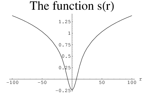
s⁡(r)=max⁡Re ​l1,12​(i​r+σ),s(r)=\max\mbox{Re~}l_{1,\frac{1}{2}}(ir+\sigma),

where the maximum is taken over σ∈[−12,32]\sigma\in[-\frac{1}{2},\frac{3}{2}].

Refer to caption
Figure 14: The graph of s⁡(r)s(r).

6.1 Criteria

If ∑j=1ns⁡(rj)<0\sum_{j=1}^{n}s(r_{j})<0 then there is no cuspidal eigenfunction in L2​(S​Ln​(ℤ)\S​Ln​(ℝ)/S​On​(ℝ))L^{2}(SL_{{n}}({\mathbb{Z}})\backslash SL_{{n}}({\mathbb{R}})/SO_{{n}}({\mathbb{R}})) whose Langlands parameters μ1,…,μn\mu_{1},\ldots,\mu_{n} have Im ​μj=rj\mbox{Im~}\mu_{j}=r_{j}.

If ϕ\phi is a cusp form, then the archimedean Ramanujan-Selberg conjectures assert that π∞\pi_{\infty} is tempered, i.e. Re ​μj=0\mbox{Re~}{\mu_{j}}=0. A consequence is that λc​u​s​p≥n3−n24\lambda^{cusp}\geq\frac{n^{3}-n}{24}. This was proven in [M] unconditionally using a similar positivity argument. Here we can derive some stronger results and different applications.

Proposition 6.1.

(A trivial bound) If ϕ\phi is a cusp form in L2​(S​Ln​(ℤ)\S​Ln​(ℝ)/S​On​(ℝ))L^{2}(SL_{{n}}({\mathbb{Z}})\backslash SL_{{n}}({\mathbb{R}})/SO_{{n}}({\mathbb{R}})), then with the above notation

∑j=1nrj2>51.84​(1+1n−1).\sum_{j=1}^{n}r_{j}^{2}>51.84\left(1+\frac{1}{n-1}\right).

Proof: The plot shows s⁡(r)<0s(r)<0 for |r|<7.2|r|<7.2. Thus ∑j=1ns⁡(rj)≥0\sum_{j=1}^{n}s(r_{j})\geq 0 only if at least one |rj|≥7.2.|r_{j}|\geq 7.2. Since the rjr_{j} are constrained to have r1+⋯+rn=0r_{1}+\cdots+r_{n}=0, this means

∑j=1nrj2≥7.22+(n−1)​(7.2n−1)2.\sum_{j=1}^{n}r_{j}^{2}\geq 7.2^{2}+(n-1)\left(\frac{7.2}{n-1}\right)^{2}.

□\Box

Theorem 1 follows immediately from Proposition 6.1 and (10).

6.2 Extreme values

Given dd and the constraints ∑rj2=d,∑rj=0\sum r_{j}^{2}=d,\sum r_{j}=0, if the largest value obtained by ∑s⁡(rj)\sum s(r_{j}) is negative, then Criteria 6.1 implies λ>d2+n3−4​n24\lambda>\frac{d}{2}+\frac{n^{3}-4n}{24}.

Principle 6.2.
33 3 Some may not consider the justification to be a proof, but as we indicate, it can be verified in the applications we use it for.

If (r1,…,rn)(r_{1},\ldots,r_{n}) is an extremal point of

∑j=1ns⁡(rj)\sum_{j=1}^{n}s(r_{j})

subject to the constraints

∑j=1nrj=0,∑j=1nrj2=d,\sum_{j=1}^{n}r_{j}=0~~,~~\sum_{j=1}^{n}r_{j}^{2}=d,

then the rjr_{j} assume at most three distinct values.

Proof: By Lagrange multipliers, there are real constants c1,c2∈ℝc_{1},c_{2}\in\mathbb{R} such that

(s′​(r1),…,s′​(rn))=c1​(r1,…,rn)+c2​(1,…,1),(s^{\prime}(r_{1}),\ldots,s^{\prime}(r_{n}))=c_{1}(r_{1},\ldots,r_{n})+c_{2}(1,\ldots,1),

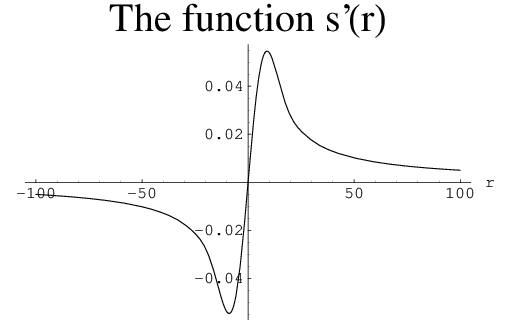
i.e. the points (rj,s′​(rj))(r_{j},s^{\prime}(r_{j})) all lie on the intersection of some line and the graph of y=s′​(x)y=s^{\prime}(x).

Refer to caption
Figure 15: The graph of s′​(r)s^{\prime}(r).

But no line crosses this graph in more than three places. Even though Figure 15 only shows the range |x|≤100|x|\leq 100 it is legal to use this principle in this paper. For another crossing would give a value of rjr_{j} so large that it would not enter into our subsequent bounds. □\Box

Theorem 6.3.

We have the following bounds on the Laplace eigenvalue of a cuspidal eigenfunction of Δ\Delta in L2​(S​Ln​(ℤ)\S​Ln​(ℝ)/S​On​(ℝ))L^{2}(SL_{{n}}({\mathbb{Z}})\backslash SL_{{n}}({\mathbb{R}})/SO_{{n}}({\mathbb{R}})):

nn 33 44 55 66 77 88
λ≥\lambda\geq 87.62587.625 108.108. 140.875140.875 167167. 201.125201.125 232.232.

Proof: By the last proposition, we need only consider the case where there are A​r1Ar_{1}’s, B​r2Br_{2}’s, and C​r3Cr_{3}’s, with r1,r2,r3∈ℝr_{1},r_{2},r_{3}\in\mathbb{R},

A​r1+B​r2+C​r3=0,A​r12+B​r22+C​r32=d,Ar_{1}+Br_{2}+Cr_{3}=0~~,~~Ar_{1}^{2}+Br_{2}^{2}+Cr_{3}^{2}=d,

and then try to find a large value of dd such that

A​s​(r1)+B​s​(r2)+C​s​(r3)As(r_{1})+Bs(r_{2})+Cs(r_{3})

is always negative. Since A,B,A,B, and CC are all positive integers which sum to nn, this is a finite calculation. We will take A,B,C>0A,B,C>0 by allowing some of the values of r1,r2r_{1},r_{2}, and r3r_{3} to coincide. Then in terms of the parameter r3r_{3}, either

r1=−A​C​r3+A​B​(−C2​r32+A⁡(D−C)+B⁡(D​r32−C​r32))A⁡(A+B)r_{1}=-{\frac{ACr_{3}+{\sqrt{AB\left(-C^{2}r_{3}^{2}+A(D-C)+B(Dr_{3}^{2}-Cr_{3}^{2})\right)}}}{A\left(A+B\right)}}

and

r2=−(B​C​r3)+A​B​(−C2​r32+A⁡(D−C​r32)+B⁡(D−C​r32))B⁡(A+B)r_{2}={\frac{-\left(BCr_{3}\right)+{\sqrt{AB\left(-C^{2}r_{3}^{2}+A(D-Cr_{3}^{2})+B(D-Cr_{3}^{2})\right)}}}{B\left(A+B\right)}}

or instead

r1=−A​C​r3+A​B​(−C2​r32+A⁡(D−C)+B⁡(D​r32−C​r32))A⁡(A+B)r_{1}={\frac{-ACr_{3}+{\sqrt{AB\left(-C^{2}r_{3}^{2}+A(D-C)+B(Dr_{3}^{2}-Cr_{3}^{2})\right)}}}{A\left(A+B\right)}}

and

r2=−(B​C​r3)+A​B​(−C2​r32+A⁡(D−C​r32)+B⁡(D−C​r32))B⁡(A+B).r_{2}=-{\frac{\left(BCr_{3}\right)+{\sqrt{AB\left(-C^{2}r_{3}^{2}+A(D-Cr_{3}^{2})+B(D-Cr_{3}^{2})\right)}}}{B\left(A+B\right)}}.

Actually, the second set of solutions and the first are interchanged upon r3↔−r3r_{3}\leftrightarrow-r_{3}, so they take the same values. For a given nn, we need only enumerate the integer triples of A,B,CA,B,C with A≥B≥C>0A\geq B\geq C>0 and plot

A​s​(−A​C​r3+A​B​(−C2​r32+A⁡(D−C)+B⁡(D​r32−C​r32))A⁡(A+B))+As\left(-{\frac{ACr_{3}+{\sqrt{AB\left(-C^{2}r_{3}^{2}+A(D-C)+B(Dr_{3}^{2}-Cr_{3}^{2})\right)}}}{A\left(A+B\right)}}\right)+
B​s​(−(B​C​r3)+A​B​(−C2​r32+A⁡(D−C​r32)+B⁡(D−C​r32))B⁡(A+B))+C​s​(r​3)Bs\left({\frac{-\left(BCr_{3}\right)+{\sqrt{AB\left(-C^{2}r_{3}^{2}+A(D-Cr_{3}^{2})+B(D-Cr_{3}^{2})\right)}}}{B\left(A+B\right)}}\right)+Cs(r3)

over the range

−A+B​DC​A+B+C≤r3≤A+B​DC​A+B+C.-{\frac{{\sqrt{A+B}}{\sqrt{D}}}{{\sqrt{C}}{\sqrt{A+B+C}}}}\leq r_{3}\leq{\frac{{\sqrt{A+B}}{\sqrt{D}}}{{\sqrt{C}}{\sqrt{A+B+C}}}}.

One finds the following values of dd work:

nn 3 4 5 6 7 8
dd 174 212 273 318 376 424

□\Box

Remark 6.4.

Theorem 1.3 shows there exists a positive constant c>0c>0 such that

λc​u​s​p−n3−n24>cn,n=1,2,….\lambda^{cusp}-\frac{n^{3}-n}{24}>cn~~,~~n=1,2,\ldots.

The argument above gives a much better constant.

6.3 Some open problems about λ1c​u​s​p​(S​Ln​(ℤ)\S​Ln​(ℝ)/S​On​(ℝ))\lambda^{cusp}_{1}(SL_{{n}}({\mathbb{Z}})\backslash SL_{{n}}({\mathbb{R}})/SO_{{n}}({\mathbb{R}}))

Conjecture 6.5.

Fix k=1,2,…k=1,2,\ldots and denote the kk-th cuspidal eigenvalue of Δ\Delta on L2​(S​Ln​(ℤ)\S​Ln​(ℝ)/S​On​(ℝ))L^{2}(SL_{{n}}({\mathbb{Z}})\backslash SL_{{n}}({\mathbb{R}})/SO_{{n}}({\mathbb{R}})) as λkc​u​s​p​(S​Ln​(ℤ)\S​Ln​(ℝ)/S​On​(ℝ))\lambda_{k}^{cusp}(SL_{{n}}({\mathbb{Z}})\backslash SL_{{n}}({\mathbb{R}})/SO_{{n}}({\mathbb{R}})). Then the sequence

{λkc​u​s​p​(S​Ln​(ℤ)\S​Ln​(ℝ)/S​On​(ℝ))−n3−n24n∣n=1,2,…}\left\{\frac{\lambda_{k}^{cusp}(SL_{{n}}({\mathbb{Z}})\backslash SL_{{n}}({\mathbb{R}})/SO_{{n}}({\mathbb{R}}))-\frac{n^{3}-n}{24}}{n}\mid n=1,2,\ldots\right\} (11)

has a limiting distribution.

Questions 6.6.

Is the sequence in (11) also bounded from above as well as from below?

7 Bounds on non-cuspidal eigenvalues

Lubotzky asked if the bound

λ≥n3−n24\lambda\geq\frac{n^{3}-n}{24}

could also hold for the entire non-zero discrete spectrum of Δ\Delta on L2​(S​Ln​(ℤ)\S​Ln​(ℝ)/S​On​(ℝ))L^{2}(SL_{{n}}({\mathbb{Z}})\backslash SL_{{n}}({\mathbb{R}})/SO_{{n}}({\mathbb{R}})), i.e. not just for cusp forms alone. Although from the point of view of automorphic forms the cusp forms are most essential, the entire discrete spectrum enters into considerations in differential geometry. In fact, there are non-constant, non-cuspidal, square-integrable residues of Eisenstein series on L2​(S​Ln​(ℤ)\S​Ln​(ℝ)/S​On​(ℝ))L^{2}(SL_{{n}}({\mathbb{Z}})\backslash SL_{{n}}({\mathbb{R}})/SO_{{n}}({\mathbb{R}})) which are discrete Laplace eigenfunctions, and they are never tempered (that is, they violate Re ​μj=0\mbox{Re~}\mu_{j}=0). The first example of one on S​Ln​(ℤ)\S​Ln​(ℝ)/S​On​(ℝ)SL_{{n}}({\mathbb{Z}})\backslash SL_{{n}}({\mathbb{R}})/SO_{{n}}({\mathbb{R}}) violating λ≥n3−n24\lambda\geq\frac{n^{3}-n}{24} occurs for n=68n=68:

Theorem 7.1.

There exists a discrete Laplace eigenfunction

ϕ∈L2​(S​L68​(ℤ)\S​L68​(ℝ)/S​O68​(ℝ))\phi\in L^{2}(SL_{{68}}({\mathbb{Z}})\backslash SL_{{68}}({\mathbb{R}})/SO_{{68}}({\mathbb{R}}))

such that

Δ​ϕ=λϕ​ϕ,λϕ≈12916.6<683−6824=13098.5.\Delta\phi=\lambda_{\phi}\phi~~,~~\lambda_{\phi}\approx 12916.6<\frac{68^{3}-68}{24}=13098.5.

Yet for n≤67n\leq 67 the bound

λ≥n3−n24\lambda\geq\frac{n^{3}-n}{24}

is valid for every non-zero discrete eigenvalue of Δ\Delta on L2​(S​Ln​(ℤ)\S​Ln​(ℝ)/S​On​(ℝ))L^{2}(SL_{{n}}({\mathbb{Z}})\backslash SL_{{n}}({\mathbb{R}})/SO_{{n}}({\mathbb{R}})).

Of course the failure of λ≥n3−n24\lambda\geq\frac{n^{3}-n}{24} at n=68n=68 is the typical case for large nn.

The key idea here is the classification of the discrete spectrum in terms of cusp forms. It was first conjectured by Jacquet [J] and later proven by Mœglin-Waldspurger [MW]. Let us now describe how discrete eigenfunctions can be constructed. Factor n=r​an=ra and let ϕ\phi be a cusp form on S​La​(ℤ)\S​La​(ℝ)/S​Oa​(ℝ)SL_{{a}}({\mathbb{Z}})\backslash SL_{{a}}({\mathbb{R}})/SO_{{a}}({\mathbb{R}}). The group S​Ln​(ℝ)SL_{n}({\mathbb{R}}) has a rank r−1r-1 parabolic subgroup PP of type (a,a,…,a)(a,a,\ldots,a) whose Levi component is

L=G​La​(ℝ)r∩S​Ln​(ℝ).L=GL_{a}({\mathbb{R}})^{r}\cap SL_{n}({\mathbb{R}}).

The cusp form ϕ\phi extends as a product to the rr copies of S​La​(ℝ)SL_{a}({\mathbb{R}}) in LL in the obvious way. Given h=(h1,…,hr)∈ℂrh=(h_{1},\ldots,h_{r})\in{\mathbb{C}}^{r} such that h1+⋯+hr=0h_{1}+\cdots+h_{r}=0, we can form a character of the split Levi component AA of PP, and the Eisenstein series E⁡(P,g,ϕ,h)E(P,g,\phi,h). If ϕ\phi has Langlands parameters μ1,…,μa\mu_{1},\ldots,\mu_{a}, then E⁡(P,g,ϕ,h)E(P,g,\phi,h) has Langlands parameters

(μ1+h1,μ2+h1,…,μa+h1⏞a,μ1+h2,…​…​…,μ1+hr,…,μa+hr⏞a⏟r​a=n).(\underbrace{\overbrace{\mu_{1}+h_{1},\mu_{2}+h_{1},\ldots,\mu_{a}+h_{1}}^{a},\mu_{1}+h_{2},\ldots\ldots\ldots,\overbrace{\mu_{1}+h_{r},\ldots,\mu_{a}+h_{r}}^{a}}_{ra=n}).

Furthermore, E⁡(P,g,ϕ,h)E(P,g,\phi,h) has a pole of order r−1r-1 at h=(r−12,r−32,…,−r−12)h=(\frac{r-1}{2},\frac{r-3}{2},\ldots,-\frac{r-1}{2}) and its r−1r-1st iterated residue there is a discrete, L2L^{2} eigenfunction of Δ\Delta. Moreover, all of them arise this way. For example, if r=1r=1 these are just cusp forms, and if a=1a=1, constant functions.

We compute that the residue’s Laplace eigenvalue is

2λ−n3−n12=−∑j=1a∑k=1r(μj+r−12−k)22\lambda-\frac{n^{3}-n}{12}=-\sum_{j=1}^{a}\sum_{k=1}^{r}\left(\mu_{j}+\frac{r-1}{2}-k\right)^{2}
=−r∑j=1aμj2−ar3−r12.=-r\sum_{j=1}^{a}\mu_{j}^{2}-a\frac{r^{3}-r}{12}.

Incidentally, Maass forms with Laplace eigenvalue 14\frac{1}{4} are known to exist on congruence quotients of S​L2​(ℝ)/S​O2​(ℝ)SL_{2}({\mathbb{R}})/SO_{2}({\mathbb{R}}). Using this procedure one may already construct a discrete residue on a congruence quotient of S​L4​(ℝ)/S​O4​(ℝ)SL_{4}({\mathbb{R}})/SO_{4}({\mathbb{R}}) which violates the λ≥43−424\lambda\geq\frac{4^{3}-4}{24} bound.

Proof of Theorem 7.1: Firstly, Hejhal (see [H]) has computed that λ1c​u​s​p(SL2(ℤ)\SL2(ℝ)/SO2(ℝ))=91.1413⋯\lambda_{1}^{cusp}(SL_{{2}}({\mathbb{Z}})\backslash SL_{{2}}({\mathbb{R}})/SO_{{2}}({\mathbb{R}}))=91.1413\cdots, corresponding to μ1=−μ2≈9.534​i\mu_{1}=-\mu_{2}\approx 9.534i. Thus the Laplace eigenvalue of a residue formed from Hejhal’s Maass form has

2​λ−n3−n12≈r⁡(181.8)−2​r3−r12,2\lambda-\frac{n^{3}-n}{12}\approx r(181.8)-2\frac{r^{3}-r}{12},

and this difference is positive for

r<6⋅181.8+1≈33.04.r<\sqrt{6\cdot 181.8+1}\approx 33.04.

For r=34r=34 we have

λ≈12916.6<683−6824=13098.5.\lambda\approx 12916.6<\frac{68^{3}-68}{24}=13098.5.

If in fact there was an example of a residue for n=r​a<68n=ra<68, with

−r∑j=1aμj2−ar3−r12<0,-r\sum_{j=1}^{a}\mu_{j}^{2}-a\frac{r^{3}-r}{12}<0,

we would necessarily have

r>−12a∑j=1aμj2+1.r>\sqrt{-\frac{12}{a}\sum_{j=1}^{a}\mu_{j}^{2}+1}. (12)

We already know that r>1r>1 since cusp forms obey the λ≥n3−n24\lambda\geq\frac{n^{3}-n}{24} bound. Thus we can restrict to the cases r≥2,a=1,…,34r\geq 2,a=1,\ldots,34. Using our pre-existing bounds for ∑μj2\sum\mu_{j}^{2} we conclude r​a≥68ra\geq 68 – see Table 1 for details.

aa r≤[68a]r\leq[\frac{68}{a}] Lower bound for −∑j=1aμj2-\sum_{j=1}^{a}\mu_{j}^{2} Upper bound for −∑j=1aμj2-\sum_{j=1}^{a}\mu_{j}^{2}
3 22 171.25 120.75
4 17 211 96.00
5 13 271.75 70.
6 11 316.5 60.
7 9 374.25 46.66
8 8 422 42.00
9 7 56.07 36.
10 6 55.10 29.16
11 6 54.27 32.08
12 5 53.55 24.
13 5 52.91 26.
14 4 52.32 17.5
15 4 51.79 18.75
16 4 51.29 20.
17 4 50.83 21.25
18 3 50.38 12.
19 3 49.96 12.66
20 3 49.56 13.33
21 3 49.18 14.
22 3 48.80 14.66
23 2 48.44 5.75
24 2 48.09 6.
25 2 47.75 6.25
26 2 47.41 6.5
27 2 47.08 6.75
28 2 46.76 7.
29 2 46.44 7.25
30 2 46.12 7.5
31 2 45.81 7.75
32 2 45.51 8.
33 2 45.20 8.25
34 2 44.91 8.5
Table 1: This table completes the proof of Theorem 7.1. Suppose a residue of a cusp form on G​LaGL_{a} occurred on some G​Ln,n=r​a<68GL_{n},n=ra<68 with Laplace eigenvalue ≤n3−n24\leq\frac{n^{3}-n}{24}. The second column gives the upper bound r≤[68a]r\leq[\frac{68}{a}]. The third column gives a lower bound for −∑j=1aμj2-\sum_{j=1}^{a}\mu_{j}^{2} (from Proposition 6.1), but the fourth gives an upper bound on −∑j=1aμj2-\sum_{j=1}^{a}\mu_{j}^{2} that would be satisfied by such a residue with low eigenvalue (as derived in (12) in the proof of Theorem 7.1). The inconsistency of these two inequalities is a contradiction which shows that the discrete Laplace spectrum on S​Ln​(ℤ)\S​Ln​(ℝ)/S​On​(ℝ)SL_{{n}}({\mathbb{Z}})\backslash SL_{{n}}({\mathbb{R}})/SO_{{n}}({\mathbb{R}}) is contained in {0}∪[n3−n24,∞)\{0\}\cup[\frac{n^{3}-n}{24},\infty) for n<68n<68.

□\Box

8 Cuspidal cohomology

The positivity inequality can be applied to products of L-functions which have poles, for example Rankin-Selberg L-functions L⁡(s,π⊗π~)L(s,\pi\otimes\tilde{\pi}) of cuspidal automorphic forms π\pi on G​LnGL_{n}. If {μj​k}j=1,k=1m\{\mu_{jk}\}_{j=1,k=1}^{m} are the archimedean Γℝ\Gamma_{\mathbb{R}} parameters, the inequality reads

∫ℝg(x)(ex/2+e−x/2)dx+2Re ∑j=1m∑k=1ml(μj​k)+g(0)logD≥0.\int_{{\mathbb{R}}}g(x)\left(e^{x/2}+e^{-x/2}\right)dx+2\mbox{Re~}\sum_{j=1}^{m}\sum_{k=1}^{m}l(\mu_{jk})+g(0)\log D\geq 0. (13)

The new term in (13) as compared to (4) comes from the poles of L⁡(s,π⊗π~)L(s,\pi\otimes\tilde{\pi}). Also, here we have simply dropped the coefficients entirely because L′L​(s,ϕ)\frac{L^{\prime}}{L}(s,\phi) has a Dirichlet series with non-positive coefficients (see [RS] for a verification of this) and so there is no restriction on the support of gg.

If π=⊗p≤∞πp\pi=\otimes_{p\leq\infty}\pi_{p} comes from a constant-coefficients cohomological cusp form on G​Ln​(𝔸ℚ)GL_{n}(\mathbb{A}_{\mathbb{Q}}) then π∞\pi_{\infty} is of either the form

π∞=IndP(2,2,…,2)G​Ln​(D2,D4,…,Dn),n​ even,\pi_{\infty}=\mbox{Ind}_{P_{(2,2,\ldots,2)}}^{GL_{n}}(D_{2},D_{4},\ldots,D_{n}),~n\mbox{ even},

or

π∞=IndP(1,2,2,…,2)G​Ln​(sgn​(⋅)ϵ,D3,D5,…,Dn),n​ odd.\pi_{\infty}=\mbox{Ind}_{P_{(1,2,2,\ldots,2)}}^{GL_{n}}(\hbox{sgn}(\cdot)^{\epsilon},D_{3},D_{5},\ldots,D_{n}),~n\mbox{ odd}.

(sgn is the sign character, ϵ=0\epsilon=0 or 1, and DkD_{k} denotes the kk-th discrete series on G​L2GL_{2}, corresponding to weight kk holomorphic forms.) Thus, if nn is written as 2​m+t2m+t, t=0t=0 or 1, the archimedean μj​k\mu_{jk} can be computed via the recipe summarized in [RS] and are the following multisets:

{μj,k}\displaystyle\{\mu_{j,k}\} =\displaystyle= {t+j+k,t−1+j+k,|k−j|,1+|k−j|∣1≤j,k≤m}\displaystyle\{t+j+k,t-1+j+k,|k-j|,1+|k-j|\mid 1\leq j,k\leq m\}
∪\displaystyle\cup {0,j,j,j+1,j+1∣1≤j≤m}⏟omit if t=0.\displaystyle~~~~~~~~~~~~~~~~~\underbrace{\{0,j,j,j+1,j+1\mid 1\leq j\leq m\}}_{\mbox{omit if $t=0$}}.
Theorem 8.1.
Hc​u​s​p⋅​(S​Ln​(ℤ),ℝ)=0,1<n<27.H^{\cdot}_{cusp}(SL_{n}({\mathbb{Z}});{\mathbb{R}})=0,~1<n<27.

Proof: Let

gp​(x)=((1−|x|p)​cos⁡(π​xp)+1π​sin⁡(π​|x|p))/cosh⁡(x/2).g_{p}(x)=\left((1-\frac{|x|}{p})\cos(\frac{\pi x}{p})+\frac{1}{\pi}\sin(\frac{\pi|x|}{p})\right)/\cosh(x/2).

Then h1,p​(r)=g^1,p​(r)h_{1,p}(r)=\hat{g}_{1,p}(r) is positive in the critical strip |Im ​r|<12|\mbox{Im~}r|<\frac{1}{2}. For our cohomological forms D=1D=1 at full level and with the μj​k\mu_{jk}’s as above we arrive at a contradiction to the positivity inequality (see Table 2). □\Box

n tt LHS(13) n tt LHS(13) n tt LHS(13) n tt LHS(13)
2 3. -2.821 15 6. -111.4 9 6. -71.43 22 6. -77.30
3 6. -8.113 16 6. -112.1 10 6. -80.27 23 6. -64.06
4 6. -17.02 17 6. -112.4 11 6. -89.68 24 6. -46.70
5 6. -28.30 18 6. -109.2 12 6. -96.45 25 6. -28.18
6 6. -38.51 19 6. -105.4 13 6. -103.4 26 6. -5.388
7 6. -50.30 20 6. -97.87 14 6. -107.5
Table 2: The (numerical) proof of the cohomology theorem. The left-hand side of (13), ∫ℝg(x)(ex/2+e−x/2)dx+2Re ∑j=1m∑k=1ml(μj​k)+g(0)logD\int_{{\mathbb{R}}}g(x)\left(e^{x/2}+e^{-x/2}\right)dx+2\mbox{Re~}\sum_{j=1}^{m}\sum_{k=1}^{m}l(\mu_{jk})+g(0)\log D must be positive if the cusp form exists, and this table shows it is negative for n<27n<27.

Remarks

We proved this for n<23n<23 in [M] with the Rankin-Selberg L-functions but without Weil’s formula (instead using the Mittag-Leffler expansion). Fermigier [F] proved a weaker result using Weil’s formula but with the standard L-function. The above theorem surpasses both.

Nothing is known about these cuspidal Betti numbers for n≥27n\geq 27, let alone if they ever non-zero.

References

  • [BDHI] Daniel Bump, W. Duke, Jeffrey Hoffstein, and Henryk Iwaniec, An estimate for the Hecke eigenvalues of Maass forms, Internat. Math. Res. Notices, 1992, No. 4, 75–81.
  • [F] S. Fermigier, Annulation de la cohomologie cuspidale de sous-groupes de congruence de G​Ln​(ℤ)GL_{n}({\mathbb{Z}}), Math. Ann. 306 (1996), no. 2, 247–256.
  • [H] D. A. Hejhal, Eigenvalues of the Laplacian for Hecke Triangle Groups, Mem. Amer. Math. Soc., 469, 1992.
  • [J] Hervé Jacquet, On the residual spectrum of G​L​(n)GL(n), in Lie group representations, II, 185–208, Lecture Notes in Math., 1041, Springer, 1984.
  • [JS] H. Jacquet and J.A. Shalika, Rankin-Selberg Convolutions: Archimedean Theory, Israel Math. Conf. Proceedings 2 (1990), 125–208.
  • [LRS] W. Luo, Z. Rudnick, and P. Sarnak, On Selberg’s Eigenvalue Conjecture, Geom. Funct. Anal. 5 (1995), no. 2, 387–401.
  • [M] Stephen D. Miller, Spectral and Cohomological Applications of the Rankin-Selberg Method, Internat. Math. Res. Notices, 1996, No. 1, 15–26.
  • [MW] C. Mœglin and J.-L. Waldspurger, Le spectre résiduel de GL⁡(n){\rm{G}{L}}(n), Ann. Sci. École Norm. Sup. (4) 22 (1989), no. 4., 605–674.
  • [O] Andrew Odlyzko, Bounds for discriminants and related estimates for class numbers, regulators and zeroes of zeta functions: a survey of recent results, Séminaire de Théorie des Nombres, Bordeaux 2 (1990), 119–141.
  • [R] W. Roelcke Über die Wellengleichungen bei Grenzkreisgruppen erster Art, Sitzungsberichte Heidelberg Akad. Wiss. (1955) NR. 4 109 pp..
  • [RS] Z. Rudnick and P. Sarnak Zeroes of Principal L-Functions and Random Matrix Theory, Duke Jour. of Math, 81 no. 2 (1996), 269–322.

Current Address:

Department of Mathematics

Hill Center-Busch Campus

Rutgers, The State University of New Jersey

110 Frelinghuysen Road

Piscataway, NJ 08854-8019

miller@math.rutgers.edu