Puzzles and (equivariant) cohomology of GrassmanniansThanks: AK is supported by the NSF and the Sloan foundation.Thanks: TT is supported by the Clay Mathematics Institute and by a grant from the Packard foundation.
Abstract.
The product of two Schubert cohomology classes on a Grassmannian has long been known to be a positive combination of other Schubert classes, and many manifestly positive formulae are now available for computing such a product (e.g. the Littlewood-Richardson rule, or the more symmetric puzzle rule from [Hon2]). Recently in [G] it was shown, nonconstructively, that a similar positivity statement holds for -equivariant cohomology (where the coefficients are polynomials). We give the first manifestly positive formula for these coefficients, in terms of puzzles using an “equivariant puzzle piece”.
The proof of the formula is mostly combinatorial, but requires no prior combinatorics, and only a modicum of equivariant cohomology (which we include). As a by-product the argument gives a new proof of the puzzle (or Littlewood-Richardson) rule in the ordinary-cohomology case, but this proof requires the equivariant generalization in an essential way, as it inducts backwards from the “most equivariant” case.
This formula is closely related to the one in [MS] for multiplying factorial Schur functions in three sets of variables, although their rule does not give a positive formula in the sense of [G]. We include a cohomological interpretation of this problem, and a puzzle formulation for it.
1. Summary of results
In [Hon2] we introduced a new rule (the puzzle rule) for computing Schubert calculus (intersection theory on Grassmannians ), and proved it by reduction to the honeycombs of [Hon1]. This reduction implicitly involved the somewhat tricky relation between this cohomology ring and the representation ring of the general linear group , and so our derivation of the puzzle rule was somewhat indirect. In this paper we give an independent and nearly self-contained proof of the puzzle rule. The proof is mainly combinatorial; the only non-combinatorial aspects are a small amount of equivariant cohomology theory and the Pieri rule (For completeness, we include a combinatorial proof of the Pieri rule in an appendix.) In particular, we avoid any use of the Littlewood-Richardson rule11 1 Indeed, one can use the results in this paper, together with the correspondences in [Hon2] and [Bu2], to prove that the Littlewood-Richardson rule computes Schubert calculus, though this is not the most direct derivation of this fact..
In the course of our argument we also give a formula for equivariant Schubert calculus on Grassmannians, that is manifestly positive in the sense of [G] (which shall be defined in a moment); to our knowledge this is the first such formula.
1.1. The puzzle rule for .
We first recall the definition of Schubert calculus, and the puzzle rule from [Hon2] which computes this calculus.
Let be fixed integers. Abusing notation, we let denote the set of strings consisting of ones and zeroes in arbitrary order, e.g. . This set has an obvious left action22 2 Readers familiar with Schubert classes on flag manifolds may wish to think of as quotiented by the right-action of . There are many suggestive hints that the arguments in this paper should extend from Grassmannians to flag manifolds, but we have so far been unable to extend them. of the permutation group . In particular, the long word acts on by reversal, e.g. . If , we define an inversion of to be a pair with . We denote the set of inversions by and the number of inversions by . Observe that in there is a unique string with no inversions, a unique string (assuming ) with one inversion, and a unique string with the maximal number of inversions.
If is a string, we let denote the corresponding coordinate -plane in , and let be the Schubert cycle in defined as
where is the anti-standard -plane. Equivalently, is the closure of the set
The Schubert class is the Poincaré dual of the cycle . In particular the degree of is . These classes are well-known to give a basis (over ) for the cohomology ring , and as such we can expand uniquely the product of any two classes as a sum over the basis , weighted by the structure constants of the multiplication. These integers are the concern of (ordinary) “Schubert calculus”.
Schubert calculus can be computed by many combinatorial rules, most famously the Littlewood-Richardson rule; we however shall use the more symmetric puzzle rule from [Hon2], which we now recall.
Define an (ordinary) puzzle piece as one of the following three plane figures with labeled edges:
- (1)
a unit triangle with all edges labeled 0
- (2)
a unit triangle with all edges labeled 1
- (3)
a unit rhombus (two unit triangles glued together along an edge), the two edges clockwise of acute vertices labeled 0, the other two labeled 1.

Note that the set of puzzle pieces is closed under rotation but not reflection (the reflection of a rhombus puzzle piece is not again a puzzle piece). See figure 1.
Define an (ordinary) puzzle as a decomposition of an equilateral triangle into triangles and rhombi, all edges labeled 0 or 1, such that each region is a puzzle piece. (Alternately, one can speak of attaching puzzle pieces together, with edges required to match up as in a jigsaw puzzle.) We will always align our puzzles to have a South side, Northwest33 3 Our definition of northwest will be at a angle to north, rather than . Similarly for southwest, etc. side and Northeast side; this forces the edges of puzzle pieces to be oriented E-W, NW-SE, or NE-SW, the triangles to be oriented upward or downward, and the rhombi to be oriented N-S, NW-SE, or SW-NE. Some examples of puzzles are pictured in figure 2.

Define a labeled equilateral triangle to be an upward-pointing equilateral triangle of some integer side-length , with the unit edges on the boundary labeled either or . Clearly every puzzle induces a labeled equilateral triangle , which we refer to as the boundary of .
Given any three strings , we let denote the labeled equilateral triangle with NW side labeled , NE side labeled , and S side labeled (all read clockwise). We also let denote the labeled equilateral triangle with NW side , NE side , and S side , all read left-to-right. If is a puzzle, we let , , be the three strings of labels of read clockwise, thus
We will also call a puzzle with boundary a -puzzle.
Our first main result shall be a new, and essentially self-contained, proof of the following theorem.
Theorem 1 (Puzzles compute Schubert calculus).
[Hon2] Let , and let be three elements of indexing Schubert classes in . Then the following (equivalent) statements hold:
- (1)
The intersection number is equal to the number of puzzles with .
- (2)
The structure constant is equal to the number of puzzles with .
- (3)
This first formulation, in terms of Schubert intersection numbers, realizes several symmetries evident in that problem. Note that the rotation of a puzzle is again a puzzle, corresponding to the fact44 4 One would also expect a similar geometric interpretation of the commutativity property ; the puzzle rule can indeed be shown to be commutative but this turns out to be much more non-trivial. that
We include here the standard proof that these integrals are a priori positive. They are visibly computing the number of signed intersection points of three Schubert cycles, perturbed to be transverse. It turns out to be possible to achieve this perturbation by replacing the standard flag by two other generic flags, which means the three transverse cycles are again complex subvarieties. Then the intersection points all have positive sign. Unfortunately this simple proof, which generalizes to arbitrary flag manifolds for arbitrary groups , does not provide a formula (under most people’s notions of “formula”).
From degree considerations we see that the structure constants vanish unless . We invite the reader to see how this simple fact can also be deduced from the puzzle rule.
If , define the dual string to be the string with all s and s exchanged; thus for instance . The dual string gives a Schubert class on the dual Grassmannian . Similarly, given a puzzle , we can define the dual puzzle by reflecting left-right and exchanging s and s everywhere. Observe that this gives a puzzle-theoretic proof of the equation
Grassmann duality gives a geometric proof of this identity, as follows. It takes a -plane to its perpendicular -plane (with respect to the standard Hermitian form on ), and the Schubert variety to the opposite Schubert variety (thinking of as the antidiagonal permutation matrix). Since the transformation is deformable to the identity transformation, again represents the Schubert class .

1.2. A new puzzle piece, for .
To prove theorem 1 we shall generalize the result so that it computes the answer to a harder question, namely the product structure in the -equivariant cohomology of Grassmannians. In section 2 we recall the (very few) necessary facts about -equivariant cohomology we need to set up this question. For now, we need only four:
- •
the equivariant cohomology ring is naturally a graded module over the polynomial ring (itself the equivariant cohomology of a point);
- •
has a natural basis of “equivariant Schubert classes” , with having degree ;
- •
there is a natural forgetful map to ordinary cohomology, which consists of setting all the to ;
- •
this forgetful map takes each equivariant Schubert class to the corresponding ordinary Schubert class .
In particular, one can speak of “equivariant Schubert calculus”, which concerns the structure constants in the product expansion55 5 In this paper, all summations over Greek indices shall range over . . By degree considerations in this graded ring, we know is a homogeneous polynomial of degree . In particular, vanishes when , and agrees with the ordinary structure constants when (which is why we can safely use the same notation for both).
It is not hard to show that the equivariant structure constants actually live in the subring . In [G] it is proven that written as polynomials in these differences, the structure constants have positive integer coefficients (this was first conjectured by Dale Peterson). As in the non-equivariant case, the proof does not directly give a formula for the .
To compute these , we need to generalize our notion of puzzle a bit. We introduce the equivariant puzzle piece: this is the same as the N-S rhombus puzzle piece but with the s and s interchanged. A puzzle using some equivariant pieces66 6 Since equivariant Schubert calculus generalizes ordinary, we can safely call these again “puzzles” and need not introduce a term “equivariant puzzles”. Rather, one might call a puzzle ordinary if one wanted to emphasize that it happens to contain no equivariant pieces. is given in figure 4.

To each equivariant piece in a puzzle, we associate a weight , which we compute by dropping lines SW and SE from the piece until they poke out the th and th place on the South side and then setting . See figure 5. The weights of the pieces in figure 4 are given as example. We can then associate a weight to every puzzle by defining , where ranges over the equivariant pieces of . (An empty product is taken to be , of course.)
Observe that we necessarily have in the above definition of . In particular, the weight of a puzzle can be expressed as a positive combination of .
The main result of this paper is
Theorem 2 (Puzzles compute equivariant Schubert calculus).
Let , and let be three elements of , indexing equivariant Schubert classes in . Then the following (equivalent) statements hold:
- (1)
The structure constant is equal to the sum of the weights of all puzzles with . In particular, we explicitly demonstrate for the abstract positivity result in [G].
- (2)
This obviously implies the second and third formulations of theorem 1. There is no close analogue of the first formulation.77 7 The closest analogue would be to compute . So a positive formula for the structure constants gives a positive formula for the integrals. The converse does not seem to be obviously true. In ordinary cohomology the three formulations could be equated via the formula , but this identity does not hold in equivariant cohomology. In particular, we should not lament the symmetry lost by including the non-rotatable equivariant piece, since the problem itself is less symmetric. On the other hand, the dual of an equivariant puzzle is still an equivariant puzzle, giving an equality , where the bar is defined by . This again follows from Grassmann duality (the two coefficients are not equal, because is not deformable to the identity through -invariant maps).
We give an example in figure 6, computing the products and . These are of course equal (the ring is commutative), but this is very nonobvious from the formula.

This paper is organized as follows. In the “geometric” part (sections 2 – 3, plus an optional Appendix) of the paper we set up the machinery from equivariant cohomology which we will need, culminating in the equivariant Pieri identities for Schubert classes and structure constants. In the “combinatorial” part (sections 4 – 5) we show that the equivariant puzzle rule obeys these Pieri identities, which will imply theorem 2 (and hence theorem 1) by an induction argument. We remark that this induction only seems to be available in the equivariant setting, so we cannot give a completely non-equivariant proof of theorem 1 by these techniques.
Finally, in section 6 we compare the results here with those in [MS] for multiplying factorial Schur functions (which are nothing other than double (i.e. equivariant) Schubert polynomials for Grassmannian permutations). They solve a different problem, which also reduces to ordinary Schubert calculus when . We introduce cohomological formulations of their problem, and a reformulation of their rule in terms of “MS-puzzles”.
2. Equivariant cohomology, especially of Grassmannians
Fix . In this section we give a combinatorial definition of the equivariant cohomology ring , which we interpret as lists of polynomials indexed by satisfying some congruence conditions. We then invoke some standard facts about equivariant cohomology to determine that this ring is indeed the ring of equivariant cohomology classes on the Grassmannian, and is equipped with a basis of equivariant Schubert classes which map to ordinary Schubert classes under the forgetful map88 8 We chose this rather odd approach to to emphasize the point that one does not actually need much equivariant cohomology theory to prove Theorem 1, and one could in fact just think of as an abstract ring of lists of polynomials to be manipulated combinatorially without ever having to understand what the functor means.. Our reference for combinatorial properties of equivariant cohomology is [GZ].
2.1. A combinatorial description of .
Begin by defining to be the polynomial ring in variables (without yet worrying what “” means in general). Define to be the space of all lists of polynomials , indexed by elements . This is clearly a commutative ring, and a -module (where acts diagonally on each term of the list).
Suppose that . Call a class if it satisfies the GKM conditions:
For each pair , differing99 9 Equivalently, we have , where is the transposition of and . only in places and , the difference should be a multiple of .
Examples. The list is a class, since all the relevant differences are . The list is also a class1010 10 Topologically, this class arises as the equivariant first Chern class of the th exterior power of the tautological -plane bundle on the Grassmannian. , where the multiples are all . For each , the list is also a class. In figure 7 are a list of some very special classes in .
Now define to be the set of all classes. It is obviously a subring and a submodule of .
Define the support of a class as the set such that . Recall that is a lattice, where the partial order is given by if one has for all . Say that is supported above if one has for all .
Let , and let be a class supported above . This forces to be a multiple of. If we have the stronger relationship , and also is homogeneous of degree1111 11 In this paper we give each generator a degree of 1, although from the cohomological considerations below it could be argued that the really deserve to have degree 2. We believe however that setting here would be too confusing. We remark that if we replaced the equivariant cohomology ring with the equivariant Chow ring (which is equivalent for ) then the genuinely do have degree 1. for all , we call a Schubert class corresponding to . For some examples, see the Schubert classes in in figure 7.
Lemma 1 (Schubert classes are unique).
For each there is at most one Schubert class corresponding to .
Proof.
Suppose for contradiction that there were two distinct Schubert classes corresponding to . Let be a minimal element of the support of the class . Since , agree on and are supported above , we have . By the GKM conditions this forces to be a multiple of . But this contradicts the fact that is homogeneous of degree . ∎
To prove existence of Schubert classes is a little trickier. We now give a topological proof that there exists a Schubert class for each . We also give a purely combinatorial proof in the Appendix.
2.2. -equivariant cohomology.
Let be a torus, and the category of topological spaces with a continuous -action, the morphisms being equivariant maps. Then -equivariant cohomology is a contravariant functor from to supercommutative1212 12 Elements of odd degree anticommute with one another, as in ordinary cohomology. In the case of interest, the Grassmannian, there are none of these anyway and the ring is therefore commutative. graded rings. We do not define it here, as all we need are a few of its properties:
- (1)
is (as promised) a polynomial ring , whose generators are given formal degree , and correspond to a basis of the dual of the Lie algebra of . In particular we can think of weights of as giving elements of (i.e. the weights are linear combinations of the ).
- (2)
If is a -invariant oriented cycle in a compact oriented manifold , then determines1313 13 In ordinary cohomology can be defined via Poincaré duality, but that is not available in equivariant cohomology. Nonetheless this should be the intuition. an equivariant cohomology class on , which we will denote . The degree of is the codimension of in . If is not in , then the pullback of to is zero.
- (3)
There is a natural “forgetful” map from , which factors as
It takes the equivariant class associated to a -invariant cycle to the ordinary Poincaré dual of in .
- (4)
Given a -space , there are two natural equivariant maps associated, , where is the set of fixed points. These induce ring homomorphisms backwards in equivariant cohomology, . In other words, the functor takes values in the category of algebras over .
Now assume that is a smooth projective variety, and acts on algebraically with isolated fixed points. (In particular, could be the Grassmannian ). Then much more is true (see [GKM]):
- (1)
is a free module over .
- (2)
has a cell decomposition by complex cells (see [BB]), corresponding to the fixed points , whose closures give a basis of equivariant cohomology as a module over . The restriction of a class to the point is the product of the weights in the normal bundle at the point .
- (3)
The forgetful map is an isomorphism on rational cohomology.
- (4)
The natural map is injective1414 14 This is very odd from the point of view of ordinary cohomology – we are restricting cohomology classes to individual points, which would seem very forgetful, but the above assertion says that we actually lose no information. The intuition should be that the equivariant cohomology of a point is very big, being a polynomial ring..
These last two statements are the most combinatorially interesting: they say that we can do all our calculations with lists of polynomials indexed by the fixed points , and then once we understand the ring , we can (if we wish) set all the generators of to zero and recover ordinary cohomology.
It remains to understand the image of inside . Given a class and a fixed point , let denote the restriction of to , so that this map is . As it turns out, this image can be characterized by the -invariant copies of inside .
Theorem.
[GKM] Let act on a smooth projective variety , with finite, and let be a -invariant inside . Then consists of two points and . If is the weight of the -action on the one-dimensional tangent space , then we have the “GKM condition”
for all classes .
Conversely, suppose that there are only finitely many -invariant ’s, and is an element of which obeys the GKM condition for every -invariant . Then lies in the image of inside .
The first statement can be proven by applying the functor to the inclusions
The converse is deeper; see [GKM].
2.3. Grassmannians.
We now apply this technology to the case of the Grassmannian , in order to verify our claimed combinatorial description of .
The torus acting in this case is the -dimensional torus , so our base ring is . This torus acts by the diagonal action on , and thus also acts on . The fixed points are just the coordinate -planes ; we shall abuse notation and refer to the fixed point simply as .
Two fixed points , are connected by a -invariant if and only if for some . If is such a , then the action of on has weight , and similarly for .
From the GKM theorem we thus see that the equivariant cohomology ring is isomorphic (both as a ring and as a -module) to the ring defined earlier combinatorially, and we shall no longer bother to distinguish the two rings.
For each , the Schubert cycle defined in the introduction is oriented and -invariant, so it induces an equivariant cohomology class . These cycles are the closures of a cell decomposition of into complex cells. At the fixed point , the weights of the action on the normal bundle of are given by , so we have . The only fixed points in are those corresponding to strings above , so is supported above . From degree considerations we see that (treating the as having degree 1), and from the first half of the GKM theorem we see that obeys the GKM conditions. Combining this with lemma 1 we see that is indeed the Schubert class corresponding to . Furthermore, we see that maps to the ordinary cohomology class under the forgetful map to ordinary cohomology.
This concludes our construction of the equivariant Schubert classes . In section 6 we will also relate these classes to factorial Schur functions, which are polynomials in many more variables1515 15 It is remarkable that these lists of polynomials can be wrapped up into individual polynomials. This can also be traced to a geometrical fact, which is that Grassmannians can be constructed as symplectic quotients of affine space. Then the Kirwan map from equivariant cohomology of affine space (a polynomial ring) maps onto the equivariant cohomology of the Grassmannian. Since we will always work with classes, rather than factorial Schur functions, we do not go into the details of this argument..
2.4. Schubert classes form a basis.
Having used topological considerations to construct the equivariant Schubert classes , we shall use a simple combinatorial argument to show that they form a basis for .
Proposition 1.
The form a -basis for . More specifically, any class can be written uniquely as an -linear combination of using only those such that for some .
Proof.
This essentially follows from the upper-triangularity of the Schubert classes with respect to the order on . We now give the details.
First, we show the are linearly independent. Suppose for contradiction that for some which are not identically zero. Among all with , we pick a which is minimal in the lattice . But then the restriction of to is , contradiction.
To see that the span, let be a class one is attempting to write as a -linear combination of some classes satisfying those conditions. Let be a minimal element of the support of . From the GKM conditions we see that must be a multiple of . Subtracting , we can inductively reduce the support of upwards until it is gone. This only uses those for which for some . ∎
Example. Consider the class , which is supported above (refer back to figure 7 to see these classes). Following the algorithm given in proposition 1 to write this in the Schubert basis, we first subtract off a multiple of itself, the multiple being . The remainder is supported at , and is in fact times . In all . This is an example of the “equivariant Pieri rule” proved in proposition 2. We verify the puzzle rule in this example, in figure 8.

Since the form a -basis of the ring , we can define structure constants for all by the formula
We record some elementary properties of these structure constants.
Lemma 2.
The structure constant has degree , and vanishes unless and . In the special case , the structure constants are integers and agree with those from ordinary Schubert calculus.
At the other extreme, when we have .
Proof.
The first claim follows since each has degree . In particular vanishes when . The class is supported above and above , so by proposition 1 we obtain the conditions . If we apply the forgetful map from equivariant cohomology to ordinary cohomology, then the structure constants of non-zero degree all vanish, leaving only those with , which explains the last claim in the first paragraph.
Finally, if we restrict to , we obtain
Since vanishes unless , and is supported above , we see that all the terms in the summation vanish. The claim then follows since is non-zero. ∎
From the above lemma we see that the equivariant structure constants compute Schubert classes when , and ordinary structure constants when . In the next section we prove a Pieri rule which bridges the gap between these two extreme cases.
3. Pieri-based recurrence relations
In this section we assume that , since the Schubert calculus for the and cases are trivial.
Let denote the unique element of with one inversion. The corresponding Schubert class is the only one of degree , coming from the unique Schubert divisor (hence the name). With , and the associativity of the equivariant cohomology ring, we will establish recurrence relations on the Schubert classes and the equivariant structure constants .
Lemma 3.
The Schubert divisor class is given by
Proof.
The right-hand side is clearly homogeneous of degree , supported above , and equals when restricted to . It can easily be shown to also obey the GKM conditions. The claim then follows from lemma 1. ∎
Write if and ; this is the covering relation in the lattice . Equivalently, if and for some strings , . Thus for instance .
Proposition 2 (The equivariant Pieri rule).
Proof.
From lemma 2 and the fact that we have
where the are the structure constants for ordinary Schubert calculus. The claim then follows from the ordinary-cohomology Pieri rule1616 16 The “Pieri rule” sometimes refers to a more general rule than we need here, for multiplying by where . The equivariant version of this rule was recently formulated [G]-positively in [R], for flag manifolds (not just Grassmannians). (as proved in [F]). ∎
In the appendix we shall give an alternative proof of proposition 2 which does not go through the ordinary Pieri rule.
The equivariant Pieri rule gives a recurrence relation on the structure constants :
Theorem 3.
[MS] For any we have the recurrence relation
The above recurrence was proven in [MS] by a different argument; it had also been observed by A. Okounkov.
Proof.
We use associativity of multiplication in and the equivariant Pieri rule to expand in two different ways:
and
Comparing coefficients of , we get
as desired. ∎
The above recurrence gives us a purely combinatorial way to verify that a putative formula for equivariant structure constants indeed works:
Corollary 1.
Let . Suppose that we have an assignment from to obeying the following identities:
- •
For any , we have
(1) - •
For any , we have
(2) - •
For any we have
(3)
Then for all , , .
The identity (1) thus involves only -puzzles, while (2) involves -puzzles and (3) involves general -puzzles.
Proof.
If or then we must have , and the claim follows from (1), Lemma 2, and the definition of . So we assume .
To begin with, we use the first two properties of to show that (which we already knew to be equal to ). We induct on the quantity , which is clearly bounded from below. If , then is non-zero, and the claim follows from (2), proposition 2, and the induction hypothesis1717 17 Observe that this induction argument implies that vanishes unless , which is of course consistent with the support properties of . Similarly, the argument in the next paragraph shows that vanishes unless . (observing that ). In the base case we instead use (1) and our definition of the class .
We can tighten this further using the duality operation on puzzles, which takes to . Also, we have , where is the involution on defined by for . From these observations and the definition of we see that
Lemma 4.
Proof.
If we thus apply (3) with replaced by and apply the involution, we obtain
From lemma 3 we have
while from the definitions we see that is equivalent to . We obtain1818 18 This could also have been obtained from (3) and the commutativity property . This commutativity property is of course true (since it manifestly holds for the ) but is non-trivial to prove using puzzles, so we rely instead on duality.
We now specialize this to the case , and use (4) to see that when . The claim (2) follows. ∎
4. SW-NE rhombi, and the proofs of (1) and (4)
We give first a “Green’s theorem” argument to constrain the interior of a puzzle from its boundary. Suppose that is a SW-NE rhombus. If we drop lines SE from , they will poke out of the th and st place of the South side of the puzzle for some . We then define the discrepancy of to be .
Lemma 5.
Let be a -puzzle. Then
Note that the edges of a SW-NE rhombus are parallel to the and sides of the puzzle.
Proof.
Let be any puzzle piece of , and let be an edge of . We give the pair a “flux” as follows. If is a -edge, or a NW-SE -edge, we set . Otherwise we drop a line SE from until it pokes out of the th place on the South side, and set , where the sign is positive if is on the SW, SE, or S side of , and negative if is on the N, NW, or NE side.
Now compute the total flux of a puzzle piece . By checking each case from Figure 1 (and the equivariant piece) in turn, we see that has total flux zero unless is a NW-SE rhombus, in which case the total flux is .
Finally, add up the flux of all the puzzle pieces in . At each internal edge, the contributions from the two pieces containing that edge cancel one another. So the total flux reduces to a sum over the edges on the boundary of , which can be computed as
Combining this with the previous paragraph we obtain the lemma. ∎
This has some very pleasant corollaries:
Corollary 2.
Let be a -puzzle.
Then all have the same number of ’s (they are elements of the same ).
Also, the number of rhombi in with edges parallel to the and sides is . Similarly when is replaced with throughout.
Proof.
For the first, specialize at . (This argument can be presented much more simply than we have done here!) For the second, specialize at . ∎
Another consequence is
Corollary 3.
Let be a -puzzle. Then:
- •
We must have and in the partial order on . (This is (4).)
- •
If , there can be no SW-NE rhombi.
- •
If , the can be no SW-NE or NW-SE rhombi.
Proof.
Since the discrepancies are all positive in the sense of [G], we see from the previous lemma that is non-negative. But this is equivalent to . Furthermore, if , then there cannot be any SW-NE rhombi, since would then be strictly positive, a contradiction.
To obtain the corresponding statements concerning , we replace by the dual puzzle defined in the introduction. (Alternatively, one can “dualize” the proof of lemma 5 by the appropriate reflection and swapping of 0-edges and 1-edges.) ∎
We now prove (1), in the form of
Proposition 3.
There exists a unique -puzzle , and its weight is .
Proof.
Define a “diamond” in a puzzle to be any of the following objects:
- •
A N-S rhombus piece;
- •
An equivariant puzzle piece;
- •
Two triangular puzzle pieces joined by an E-W edge.
Note that the NW label on a diamond matches that on the SE, likewise the NE and SW labels match.
Let be a -puzzle. By the third conclusion of Corollary 3, contains no SW-NE or NW-SE rhombi. Thus we can cut along all NW-SE and NE-SW lines without slicing through any rhombi. Except for the triangles attached to the South side, the sliced-up falls into diamonds.
We analyze starting from the bottom. First, attach the isolated
triangles. Then in each trough, fill in the unique diamond that
fits. We give the example of .
![[Uncaptioned image]](0112150v1/lamlamlamex.png)
Layer by layer, this creates the only puzzle with S edge (read left to right) that uses no NW-SE or NE-SW rhombi. By the matching properties of diamonds, the NW and NE edges also end up labeled . This shows the existence and uniqueness.
An equivariant piece comes whenever the trough to be filled has a on the SE and on the SW, coming from an inverted and in . This shows that the weight is as advertised. ∎
5. Gashed puzzles: the proof of (3)
We give first the crucial definition, and then a rough indication of the argument.
Definition.
We define a gashed puzzle as a decomposition of a labeled equilateral triangle into a collection of puzzle pieces, along with a line segment in the triangular lattice (which we refer to as the gash), such that
- •
The gash is contained in the equilateral triangle (either on the boundary or in the interior), and is oriented either E-W or SW-NE;
- •
every edge not on the gash has at most one label (as in a non-gashed puzzle)
- •
if the gash is oriented SW-NE, then it is length , and the labels on each side are a then a (read clockwise)
- •
if the gash is oriented E-W, then it is length at least , with all but the first and last edge passing through the short diagonals of some equivariant rhombi. The labels on each side are a , then the short diagonals of some equivariant rhombi, then (read clockwise).

Some examples of gashed puzzles appear in figure 9. As with non-gashed puzzles, we can define the weight of a gashed puzzle to be the product of the weights of all the equivariant pieces . Thus for instance the second puzzle in figure 9 has weight .
We now give an extremely rough indication of the argument, which decomposes (3) into the four identities (5)-(8) to come. Recall that equation (3) computes from for and for . We will take puzzles with boundary and attach a gash on their NW side, changing the boundary labels to . (This will eventually give equation (5).)
Then we will use some local rules for propagating a gash through a gashed puzzle (the map in proposition 4, giving equation (8)), preserving the weight. The gash will usually come out on the S side, and when removed it leaves a puzzle with boundary (equation (6)). If the gash always makes it through, then (the right-hand side of (3)) will be zero. This occurs in the example given in figure 10, and therefore .

Frequently though, an equivariant piece can cause a gash to heal (or appear) on its own, and (by (7)) these extra terms will give the left-hand side of equation (3). The example appears in figure 11.

Fix . We define the set to be the collection of all gashed puzzles with . We define four subsets of (local pictures given in figure 12):

We define to be the union of the (obviously disjoint) sets and , and to be the union of the (obviously disjoint) sets and . (The sets and may intersect.)
Our proof of (3) will come down to four identities. Two are very simple:
| (5) | ||||
| (6) |
We begin with (5). Let be an arbitrary element of . Then lies on a pair of edges where reads 10. If one removes the gash, one obtains a non-gashed puzzle with boundary , where is equal to but with 10 replaced by 01. In particular, we have . This argument can be reversed; given any -puzzle with , we can take the two edges where and disagree, and swap them to create a gashed puzzle . Since this affects no equivariant pieces, one has , and (5) follows.
The proof of (6) is exactly the same, except for one minor subtlety: observe that if then the gash must have length 2, since does not contain the short diagonal of any equivariant rhombus pieces.
The other two identities
| (7) | ||||
| (8) |
are more subtle and will be proved in the next two subsections.
5.1. Proof of (7).
To prove (7) we need to introduce the notion of a scab. Let be a puzzle. We define a left-scab of to be any pair of puzzle pieces in consisting of an SW-NE rhombus sitting atop a downward -triangle. Similarly define a right-scab of to be any pair of puzzle pieces in consisting of an upward -triangle sitting atop a SW-NE rhombus.
We define the weight of the scab by , where is the unique equivariant piece which can fit inside the region occupied by .
Lemma.
We have
and
Proof.
Let be a gashed puzzle in . Then must be
a NE-SW line segment of length 2, whose SW edge is the SE edge of an
equivariant piece . From Figure 1 we thus see
that there must be a downward 1-triangle between and the NE
edge of , as in figure 12.
Observe that if we replace and with a left-scab
, we obtain an ungashed puzzle with and .
![[Uncaptioned image]](0112150v1/ungashing.png)
This procedure can be reversed; given any ungashed puzzle with , and given any left-scab of , we can replace the scab with an equivariant piece and a downward 1-triangle , creating a gashed puzzle with and . This proves the first claim.
The second claim is similar (indeed, it is essentially a rotation of the first claim) and is left to the reader. ∎
The argument above motivates the terminology; when a gash closes up it leaves a scab, and conversely, a scab can come off producing a new gash.
From the above lemma, we see that to prove (7) it will suffice to show
Lemma.
Let be a -puzzle. Then
Proof.
This is another Green’s theorem argument. Let be any puzzle piece of , and let be an edge of . We give the pair a “flux” as follows. If is a -edge, or a NW-SE -edge, we set . If is an E-W -edge, we drop a line SW from until it pokes out of the th place on the South side, and set if is on the N side of , and if is on the S side of . Similarly, if is a SW-NE -edge, we drop a line SE from until it pokes out of the th place on the South side, and set if is on the NW side of , and if is on the SE side of .
Now compute the total flux of a puzzle piece . By checking each case from Figure 1 (and the equivariant piece) in turn, we see that has total flux zero unless is a -triangle. Furthermore, if is an upward -triangle sitting atop the south boundary , then also has total flux 0. Finally, if is an upward -triangle sitting atop a downward -triangle , then the total flux of and is zero.
Thus the only upward -triangles which have non-zero flux are those which sit atop SW-NE rhombi. But in that case belongs to a right-scab , and the total flux of can be easily computed to equal . Similarly, only the downward -triangles which have non-zero flux are those which sit below SW-NE rhombi, so they belong to a left-scab , and the total flux of can be easily computed to be .
Finally, add up the flux of all the puzzle pieces in . At each internal edge, the contributions from the two pieces containing that edge cancel one another. So the total flux reduces to a sum over the edges on the boundary of , which can be computed as
Combining this with the previous paragraph we obtain the lemma. ∎
Proof of (7).
This follows from the two lemmata just proven:
∎
5.2. Proof of (8).
Proposition 4.
There exists a weight-preserving bijection from to .
Proof.
Let be an element of . We shall construct an element of for which . This will require only a local surgery on , in which some pieces are replaced and the gash moves.1919 19 It is worth noting, for readers cognizant of the “gentle path” technology of [Hon2], that the center of the gash always moves along a gentle path. Indeed, the loop-breathing in [Hon2] can be interpreted as introducing a “double gash” crossing the gentle loop, propagating one gash around the loop, and once it gets back removing them both.
Suppose first that is a SW-NE gash, and consider the pieces
to its right, with a vertex on the center of the gash.
Since , there cannot be an
equivariant piece immediately to the right of , which
leaves three possibilities:
![[Uncaptioned image]](0112150v1/SWNEgash1.png)
In each of these cases, we remove the pieces and gash,
and replace them as follows:
![[Uncaptioned image]](0112150v1/SWNEgash2.png)
In each case, the labels on the boundary do not change, which means that the new set of pieces and gash match fit into the puzzle where the old ones were. So this creates a new gashed puzzle , and this is how we define .
Now take the case that is an E-W gash. Since we see that is not on the edge of the puzzle.
Suppose first that has length 2, and consider the pieces below
with a vertex on the center of the gash. There are four possibilities,
which we give below, along with their replacements in :
![[Uncaptioned image]](0112150v1/EWgash.png)
Now suppose that has length . Then the two extreme edges of
are separated by equivariant pieces as shown below (with ):
![[Uncaptioned image]](0112150v1/5widegash.png)
Observe that between and below any two equivariant pieces on the gash
there must be another equivariant piece (since nothing else can fit in
that space). That leaves possibilities for the ends, depending
on whether there are more equivariant pieces in that row below.
In each case we move the
gash down one step, possibly stretching it or shrinking it by length 1:
![[Uncaptioned image]](0112150v1/EWgashprop.png)
(In these pictures the gash begins length 4, and ends length 5, 4, 4, or 3.) This creates a new gashed puzzle , with which we define .
We have now defined for all . A simple examination of all cases verifies that is a gashed puzzle with , and also . It is obvious that since no equivariant pieces are created, destroyed, or moved.
If we rotate these local-replacement recipes by , we get a similar map from to . This is easily checked to be the inverse of , which is therefore a bijection. ∎
One can use the same rules to define a correspondence between and , but they must be iterated. This was the viewpoint of the examples in figures 10 and 11 at the beginning of the section.
Proof of theorem 2.
There is one foolish subtlety in obtaining the second statement of the theorem: the first statement (and the recurrences (2)-(3)) only constrain for all having the same number of s, and so a priori we might worry that the product might be miscalculated to have some extra terms in which has a different number of s. But by corollary 2 above, the number of s is the same on all sides of a puzzle. The second statement follows. ∎
6. The Molev-Sagan problem
In this section we compare the results of this paper with the earlier work in [MS], which was a major source of inspiration for this paper. We also give a homological (or “geometrical”) interpretation of the structure constants computed in [MS].
The paper [MS] is concerned with multiplying “factorial Schur functions” for . These functions are polynomials in two sets of variables , and are related to the classes by
Proof.
The problem solved in [MS] is more general than the one we have stated: they consider the mixed structure constants , which are polynomials in variables and , given by the product expansion
The reduce to the structure constants for equivariant cohomology of Grassmannians at the specialization (and to ordinary cohomology at ).2020 20 In [MS] they also permit to be a skew Schur function, not just a Schur function, but we have not been able to find any cohomological interpretation of these.
The formula in [MS] writes as a sum over “barred tableaux,” each one contributing a certain product . In that sense their formula is positive (and reduces to the Littlewood-Richardson rule, in the case that ). Unfortunately, many of their terms have factors with , as the example
already shows. For this reason, the computation of Molev-Sagan structure constants is too general a setting for finding a formula (as in theorem 2) for equivariant Schubert calculus that is manifestly positive in the sense of [G].
We now give a cohomological interpretation of the structure constants , which we christen “triple Schubert calculus”, and sketch how one can also compute these co-efficients using “MS-puzzles”. (Cohomology does not explicitly appear in [MS] – they consider the computation of the purely as a combinatorial question.)
6.1. Double Schubert calculus vs. equivariant Schubert calculus.
In this subsection we recall the (well-known) connection between double Schubert calculus and equivariant Schubert calculus. In a nutshell, the connection is that for any partial flag manifold , taking equivariant Schubert classes to “double Schubert classes”. We begin by recalling some standard material on double Schubert calculus (originally defined in [LS]), and its geometric interpretation.
Let denote the space of flags (i.e. maximal chains of subspaces) in . This has a transitive action of induced from its action on , and the stabilizer of the standard flag is the upper triangular matrices , so .
If we denote the lower triangular matrices by , then the Schubert cells on the Grassmannian are exactly the orbits, whose Poincaré duals gave us the Schubert basis of ordinary cohomology . These were indexed by patterns recording the intersection of the -plane with the anti-standard flag.
Analogously, we can consider closures of the -orbits on , which are again indexed by (recording the intersection of the -plane with the flag, which is now varying). The Poincaré duals of these -orbit closures then form an -basis for as varies over .
Since is a ring as well as an -module, we can define structure constants for the multiplication:
The computation of the is the concern of double Schubert calculus, and has the following homological interpretation. Fix a generic element of . The class corresponds to an irreducible cycle of pairs where satisfies two intersection conditions with : intersects -much, and intersects -much. The class corresponds to a union of cycles, each of which put only one condition on (that it intersect -much), while also requiring that live in a cycle Poincaré dual to . So the equation requiring these two to be homologous is somehow splitting the double burden on to a single burden on and a single burden on .
Restricting to , each maps to , which shows that these generalize the structure constants of ordinary Schubert calculus. This was also true of the structure constants of equivariant Schubert calculus, and like them, the carry a degree.2121 21 However, this degree is the degree of a cohomology class rather than a polynomial, and to be precise it is rather than .
We can connect double Schubert calculus with equivariant Schubert calculus using the following property of equivariant cohomology: if acts on , and ’s action is free, then . Letting denote the stabilizer of the standard -plane , so , we thus have
where we have used the fact that is isomorphic to quotiented by the diagonal action of . Thus the structure constants for equivariant Schubert calculus live in , and the forgetful map from to maps these constants to the double Schubert calculus constants .
To summarize the above discussion, while equivariant Schubert calculus essentially lacks a definition in terms of intersecting cycles, one is provided by double Schubert calculus, of which equivariant Schubert calculus is a refinement.2222 22 One can show that it is the only such refinement satisfying some natural stability properties in the limit . This is perhaps a bad way to see things, though, since such a limit can only be defined for classical Lie groups, whereas double and equivariant Schubert calculus can be defined for arbitary Lie groups.
6.2. Triple Schubert calculus.
Consider the cohomology ring as a module over the cohomology ring of the first and third factors. Since the classes form a basis of , we see that the classes form a -basis for . One could compute the structure constants for multiplication in this basis, but one would just obtain the double Schubert constants again (or to be pedantic, we would obtain ).
Since , the classes induce a corresponding basis for . The classes thus form another -basis for . Again, the structure constants for this basis are no richer than for double Schubert calculus.
In [MS] the authors (implicitly) considered the hybrid problem of computing the structure constants in the expansion
This has the following homological interpretation. We are now looking for triples . The left side of the equation says that intersects -much and also intersects -much. The right side is a union of cycles, in each of which intersects -much, has no condition directly relating to , and instead and are related by a condition Poincaré dual to . Again, the equation is shifting the double burden on to a single burden on and a single burden on the pair .
In analogy with double Schubert calculus we feel it is appropriate to dub the computation of the triple Schubert calculus. Note that these ’s are not symmetric in and , and only become so when restricted to the flag manifold sitting diagonally in the first and third factor.
It is worth noting that triple Schubert calculus has many extensions – e.g. -theory, replacing the Grassmannian by a flag manifold, or using groups other than .2323 23 It seems difficult to formulate the notion of positivity for groups other than ; in [MS] the roots of are implicitly seen as a specialization of , and it is unclear how to extend this to arbitrary root systems. For many of the other extensions, no satisfactory explicit combinatorial formula for the structure constants is known. In this way, one can view [MS] as establishing a positivity result for triple Schubert calculus on Grassmannians.2424 24 Much as [Bu] did for K-theoretic Schubert calculus on Grassmannians. In both cases, they gave a formula directly rather than an abstract reason for positivity such as the one given in [G] for equivariant Schubert calculus.
6.3. An alternate interpretation: equivariant double Schubert calculus.
For completeness, we use the connection between double Schubert calculus and equivariant Schubert calculus discussed in subsection 6.1 to recast triple Schubert calculus as “equivariant double Schubert calculus”.
Inside , we have two interesting families of subvarieties parameterized by : the diagonal- orbit closures, and the varieties corresponding to the Schubert cycles . Both families are invariant under the diagonal action of the torus, and so define families of equivariant cohomology classes in . Either family gives a -basis of . Therefore we can expand the product
where the coefficients live in . Following a similar analysis as in subsection 6.1 one can show that these coefficients refine the coefficients in triple Schubert calculus.
The results of [MS] have the rather surprising consequence that the constants and can be lifted beyond their respective rings and to actual double polynomials ; this would suggest (speaking loosely) that one should be able to replace the cohomology ring with the “doubly equivariant” ring (using an ineffective action of on ). While this can indeed be done, the homological perspective is lost, because the classes being multiplied are no longer representable by subvarieties.
6.4. MS-puzzles solve the Molev-Sagan problem.
Define an MS-puzzle as an arrangement of puzzle pieces forming a diamond of size , looking something like a very large equivariant piece. They therefore have the usual NW and NE boundaries, and now SW and SE boundaries as well. We will require the labels on the NE boundary (read clockwise) to be the inversion-free string . Some examples are in figure 13.
Define the MS-weight of an equivariant piece as , where measures the distance from the SE side and from the SW side2525 25 This definition of weight does not reduce to the definition we needed for (non-MS) puzzles, in the case that the equivariant piece is in the top half. The definition that would do that would be for the distance from the SW side and the distance from the NW side. (starting from 1), and the weight of an MS-puzzle as the product of the MS-weights of its equivariant pieces.
Theorem.
The Molev-Sagan structure constant is equal to the sum of the weights of the MS-puzzles with on the SW side, on the NW side, and on the SE side, all read bottom-to-top. (The NE side has all s, then all s, read clockwise.)
We will not prove the theorem here, except to say that the Molev-Sagan structure constants satisfy a recurrence similar to that in corollary 1, and the MS-puzzle formula can be shown to satisfy this recurrence through a slight variant of the arguments in section 5.
Of course, similar recurrences were proven in [MS] using barred tableaux. It is possible, though quite unpleasant, to establish a weight-preserving bijection between MS-puzzles and Molev-Sagan barred tableaux, but we will not present one here.
An example of MS-puzzles in action is in figure 13, demonstrating the equality
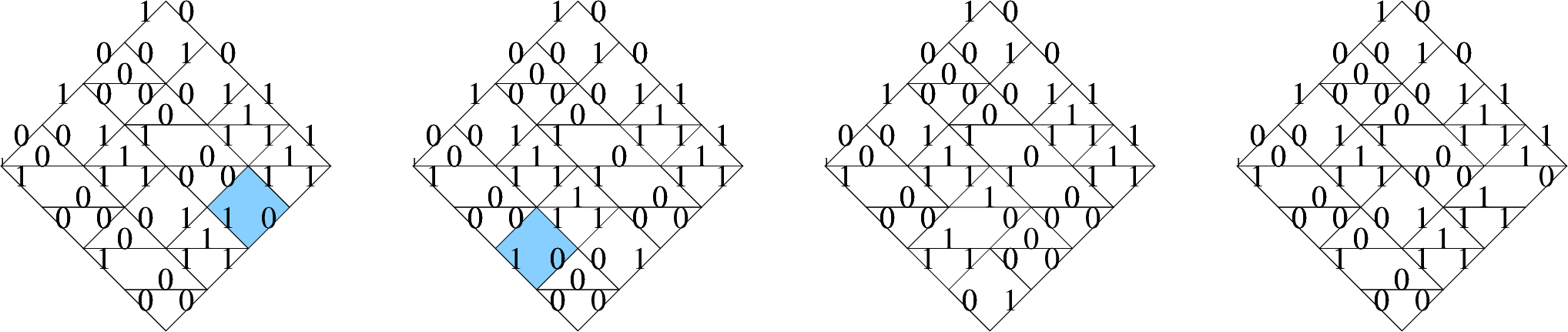
It is interesting to compare this calculation to that of using (non-MS) puzzles, as done in figure 14, which only uses three puzzles.

The fact that equivariant Schubert calculus and Molev-Sagan structure constants both reduce to ordinary Schubert calculus, in the case , is reflected in the fact that the two ordinary puzzles in the second calculation occur as the lower halves of the corresponding MS-puzzles (rotated ).
7. Appendix: existence of Schubert classes, and the equivariant Pieri rule
In this appendix we extend the standard combinatorial proof of existence of Schubert classes (via divided difference operators) to equivariant Schubert classes.2626 26 This essentially follows Demazure’s work [D], which was implicitly a calculation in equivariant K-theory localized at the fixed points of the flag manifold. Recall that, before, we established the existence of equivariant Schubert classes by direct topological means, but this did not give a formula for restrictions to fixed points. As a corollary of the formula we get a direct proof of the equivariant Pieri rule (which then implies ordinary Pieri rule as a corollary).
The permutation group acts on and on in obvious ways. If is a class, and , put these actions together to define by
which is easily seen to again be a class (i.e. satisfies the GKM divisibility conditions). We will care most about the case .
We now define the divided difference operators . If is a class, define by
A priori, this is just a list of rational functions. But in fact these turn out to define endomorphisms of (as a vector space):
Lemma.
If is a class, then is also a class.
Proof.
From the GKM conditions we see that . We want to know that itself satisfies the GKM conditions, i.e. that is a multiple of if differ in only the positions. Plainly this is true if , (or vice versa) since then the difference is zero. Otherwise, the division by is irrelevant since its GCD with is one, and then the divisibility follows from the fact that and are both classes. ∎
Recall that in section 2.3 we gave a topological proof of the existence of Schubert classes (which we already knew by lemma 1 to be unique). The first conclusion in the following lemma gives a combinatorial proof, using divided difference operators, and the second conclusion will be used in the proof of equivariant Pieri.
Lemma 6.
Fix and .
If (i.e. ), then .
If however (i.e. ), then .
In particular, one can construct the Schubert class by starting with the class (which is trivial to compute) and applying successive divided difference operators.
Proof.
The class is supported above , which implies that is supported inside . On the other hand, from degree considerations is a linear combination of Schubert classes of degree at most . From these two facts and Proposition 1 we see that must vanish if , and is an integer multiple of if . In the latter case, we can show this multiple is 1 by the straightforward computation
∎
We can now prove the equivariant Pieri rule directly.
Proposition (The equivariant Pieri rule).
Proof.
If , then they must differ in only two spots , where has and has . Applying , we get
By lemma 6 we have , hence , and
Also we have and in the above summation. The claim follows. ∎
Applying the forgetful map to ordinary cohomology we recover the ordinary Pieri rule .
References
- [BB] A. Białynicki-Birula, Some properties of the decompositions of algebraic varieties determined by actions of a torus. Bull. Acad. Polon. Sci. Sér. Sci. Math. Astronom. Phys. 24 (1976), no. 9, 667–674.
- [Bu] A. Buch, A Littlewood-Richardson rule for the K-theory of Grassmannians. To appear in Acta. Math. math.AG/0004137
- [Bu2] A. Buch, The saturation conjecture (after A. Knutson and T. Tao). With an appendix by William Fulton. Enseign. Math. (2) 46 (2000), no. 1-2, 43–60. math.CO/9810180
- [D] M. Demazure, Désingularisation des variétés de Schubert généralisées. Ann. Sci. École Norm. Sup. (4) 7 (1974), 53–88.
- [F] W. Fulton, Young tableaux. With applications to representation theory and geometry. London Mathematical Society Student Texts, 35. Cambridge University Press, Cambridge, 1997.
- [G] W. Graham, Positivity in equivariant Schubert calculus. Duke Math. J. 109 (2001), no. 3, 599–614. math.AG/9908172
- [GKM] M. Goresky, R. Kottwitz, R. MacPherson, Equivariant cohomology, Koszul duality, and the localization theorem. Invent. Math. 131 (1998), no. 1, 25–83.
- [GZ] V. Guillemin, C. Zara, Equivariant de Rham theory and graphs. Asian J. Math. 3 (1999), no. 1, 49–76. math.DG/9808135
- [Hon1] A. Knutson, T. Tao, The honeycomb model of GL(n) tensor products I: proof of the saturation conjecture. Journal of the AMS, 12 (1999), no. 4, 1055–1090. math.RT/9807160
- [Hon2] A. Knutson, T. Tao, C. Woodward, The honeycomb model of GL(n) tensor products II: puzzles give facets of the L-R cone. To appear in Journal of the AMS. math.CO/0107011
- [LS] A. Lascoux, M. Schützenberger, Interpolation de Newton á plusieurs variables. Lecture Notes in Math., 1146, 161–175, Springer, Berlin, 1985.
- [MS] A. I. Molev, B. Sagan, A Littlewood-Richardson rule for factorial Schur functions. Trans. Amer. Math. Soc. 351 (1999), no. 11, 4429–4443. q-alg/9707028
- [O] A. Okounkov, Quantum immanants and higher Capelli identities, Transformation Groups 1 (1996), 99–126. q-alg/9602028
- [R] S. Robinson, A Pieri-type formula for the equivariant cohomology of the flag manifold. To appear in the Journal of Algebra.