HOMOLOGY OF GAUSSIAN GROUPS

Our notations follow those of [37] on the one hand, and those of [22] and [20] on the other hand. Let $M$ be a monoid. We say that $x$ is a left divisor (resp. a proper left divisor) of $y$ in $M$, denoted $x\mathrel{\scriptstyle\sqsubseteq}y$ (resp. $x\mathrel{\scriptstyle\sqsubset}y$), if $y=xz$ holds for some $z$ (resp. for some $z$ with $z\not=1$). Alternatively, we say that $y$ is a right multiple of $x$. Right divisors and left multiples are defined symmetrically (but we introduce no specific notation).

Note that, if $M$ is a left Noetherian monoid, there is no invertible element in $M$ but $1$, and, therefore, the relation $\mathrel{\scriptstyle\sqsubset}$ is a strict ordering on $M$ (and so is the symmetric right divisibility relation). For $x$, $y$ in $M$, we say that $z$ is a least common left multiple, or left lcm, of $x$ and $y$, if $z$ is a left multiple of $x$ and $y$, and every common left multiple of $x$ and $y$ is a left multiple of $z$. If $z$ and $z^{\prime}$ are two left lcm’s for $x$ and $y$, then we have $z\mathrel{\scriptstyle\sqsubseteq}z^{\prime}$ and $z^{\prime}\mathrel{\scriptstyle\sqsubseteq}z$ by definition, hence $z=z^{\prime}$ whenever $M$ is left Noetherian. Thus, in a left Noetherian monoid, left lcm’s are unique when they exist.

If $M$ is a locally left Gaussian monoid, and $x$, $y$ are elements of $M$ that admit at least one common left multiple, we denote by $x\vee y$ the left lcm of $x$ and $y$, and by ${x}_{\!/\!{y}}$ the unique element $z$ satisfying $zy=x\vee y$; the latter is called the left complement of $x$ in $y$. Thus we have

whenever $x$ and $y$ have a common left multiple. Observe that, if $y$ happens to be a right divisor of $x$, then ${x}_{\!/\!{y}}$ is the corresponding quotient, i.e., we have $x={x}_{\!/\!{y}}\cdot y$: this should make the notation natural. It is easy to see that, in a locally left Gaussian monoid $M$, any two elements $x$, $y$ admit a right gcd, i.e., a common right divisor $z$ such that every common right divisor of $x$ and $y$ is a right divisor of $z$; then $M$ equipped with right division is an inf-semi-lattice with least element $1$.

The notion of a (locally) right Gaussian monoid is defined symmetrically in terms of right Noetherianity, left cancellativity and existence of right lcm’s. If $M$ is a (locally) right Gaussian monoid, and $x$, $y$ are elements of $M$ that admit a common right multiple, we denote by ${}_{x\!\backslash}\!y$ the unique element of $M$ such that $x_{x\!\backslash}\!y$ is the right lcm of $x$ and $y$, and call it the right complement of $x$ in $y$ (we shall need no specific notation for the right lcm in this paper).

Finally, we introduce Gaussian monoids as those monoids satisfying the previous conditions on both sides:

Roughly speaking, Gaussian monoids are those monoids where a good theory of divisibility exist, with in particular left and right lcm’s and gcd’s for every finite family of elements. Locally Gaussian monoids are similar, with the exception that the lcm’s operations, and, therefore, the associated complements operations, are only partial operations. The Artin monoid associated with an arbitrary Coxeter matrix is a typical example of a locally Gaussian monoid [8]; such an Artin monoid is Gaussian if and only if the associated Coxeter group is finite, i.e., in the so-called spherical case. We refer to [32] and [21] for many more examples of (locally) Gaussian monoids. Let us just still mention here the Baumslag-Solitar monoid $\langle a,b\,;\,ba=ab^{2}\rangle^{\scriptscriptstyle+}$, another typical example of a locally left Gaussian monoid that is not Gaussian, as the elements $ab$ and $a$ have no common left multiple.

If $M$ is a Gaussian monoid, it satisfies Ore’s conditions [ClP] and, therefore, it embeds in a group of fractions. We say that a group $G$ is Gaussian if there exists at least one Gaussian monoid $M$ such that $G$ is the group of fractions of $M$. The example of Artin’s braid groups $B_{n}$, which is both the group of fractions of the monoid $B_{n}^{+}$ [27] and of the Birman-Ko-Lee monoid $B\!K\!L_{n}^{+}$ [6] shows that a given Gaussian group may be the group of fractions of several non-isomorphic Gaussian monoids—as well as of many more monoids that need not be Gaussian [32].

In the sequel, we shall be specially interested in finitely generated (locally) Gaussian monoids. Actually, we shall consider a stronger condition, namely admitting a finite generating subset that is closed under some operations.

As is shown in [20], Garside monoids may be characterized by weaker assumptions: for instance, a sufficient condition for a Gaussian monoid to be Garside is to admit a finite generating subset closed under left complement. Another equivalent condition is the existence of a Garside element, defined as an element $\Delta$ such that the left and right divisors of $\Delta$ coincide, they are finite in number and they generate $M$. In this case, the family ${\mathcal{D}}_{\!{}_{\Delta}}$ of all divisors of $\Delta$ is a finite generating set that is closed under left and right complement, left and right lcm, and left and right gcd. In particular, ${\mathcal{D}}_{\!{}_{\Delta}}$ equipped with the operation of left lcm and right gcd (or of right lcm and left gcd) is a finite lattice, with minimum $1$ and maximum $\Delta$, and this lattice completely determines the monoid $M$. It is also known that every Gaussian monoid admits a unique minimal generating family, which implies that it admits a unique minimal Garside element, for instance the fundamental element $\Delta_{n}$ in the case of the monoid $B_{n}^{+}$ of positive braids. Let us mention that no example of a Gaussian non-Garside monoid of finite type is known.

Locally Garside monoids need not possess a Garside element $\Delta$ in general. Typical examples are free monoids and, more generally, FC-type Artin monoids [3]. In the cas of a free monoid ${\mathcal{X}}^{*}$ (the set of all words over the alphabet ${\mathcal{X}}$), the set ${\mathcal{X}}$ is a generating set that is trivially closed under lcm and complement: any two distinct elements $x$, $y$ of ${\mathcal{X}}$ admit no common multiple, so $x\vee y$ and ${x}_{\!/\!{y}}$ trivially belong to ${\mathcal{X}}$ when they exist, i.e., never.

In the sequel we need a convenient lcm calculus. As already pointed out in [22, 20], the main object here is not the lcm operation, but rather the derived complement operation and the algebraic identities it satisfies.

Thus, the iterated complement operation is defined by the equality

Observe that (1.1) remains true for $n=0$ provided we define ${x}_{\!/\!{Y}}$ to be $x$ if $Y$ is the empty sequence.

The constructions we shall describe in Sections 2 and, partly, 3, rely on a word process called word reversing. It was introduced in [17], and investigated more systematically in Chapter II of [19]—see also [21] for further generalizations.

If $({\mathcal{X}},{\mathcal{R}})$ is a monoid presentation, i.e., a set of letters plus a list of relations $u=v$ with $u$, $v$ words over ${\mathcal{X}}$, we denote by $\langle{\mathcal{X}}\,;\,{\mathcal{R}}\rangle^{\scriptscriptstyle+}$ the associated monoid, and by $\langle{\mathcal{X}}\,;\,{\mathcal{R}}\rangle$ the associated group. If $u$, $v$ are words over ${\mathcal{X}}$, we shall denote by $\overline{u}$ the element of the monoid $\langle{\mathcal{X}}\,;\,{\mathcal{R}}\rangle^{\scriptscriptstyle+}$ represented by $u$, and we write $u\equiv v$ for $\overline{u}=\overline{v}$. We use ${\mathcal{X}}^{*}$ for the free monoid generated by ${\mathcal{X}}$, i.e., the set of all words over ${\mathcal{X}}$; we use $\varepsilon$ for the empty word. We also introduce ${\mathcal{X}}^{-1}$ as a disjoint copy of ${\mathcal{X}}$ consisting of one letter $\alpha^{-1}$ for each letter $\alpha$ of ${\mathcal{X}}$. Finally, we say that the presentation $({\mathcal{X}},{\mathcal{R}})$ is positive if all relations in ${\mathcal{R}}$ have the form $u=v$ with $u$, $v$ nonempty, and that it is complemented if it is positive and, for each pair of letters $\alpha$, $\beta$ in ${\mathcal{X}}$, there exists at most one relation of the form $v\alpha=u\beta$ in ${\mathcal{R}}$, and no relation $u\alpha=v\alpha$ with $u\not=v$.

For further intuition, it is important to associate with every reversing sequence starting with a word $w$ a labelled planar graph defined inductively and analogous to a van Kampen diagram: first we associate with $w$ a path labelled by the successive letters of $w$, in which the positive letters (those in ${\mathcal{X}}$) are given horizontal right-oriented edges and the negative letters (those in ${\mathcal{X}}^{-1}$) are given vertical down-oriented edges. Then, word reversing consists in inductively completing the diagram by using a relation $v^{\prime}u=u^{\prime}v$ of ${\mathcal{R}}$ (or a trivial relation $u=u$) to close a pattern of the form into .

In general, word reversing is not a deterministic process: starting with one word may lead to various sequences of words, various diagrams, and, in particular, to several terminal words, the latter being those words that contain no pattern $\alpha\alpha^{-1}$ or $\alpha\beta^{-1}$ such that there exists at least one relation $v\alpha=u\beta$ in ${\mathcal{R}}$. However, it is easily shown that, if ${\mathcal{R}}$ is a complemented presentation, then there exists a unique maximal reversing diagram starting with a given word $w$, and $w$ is reversible to at most one terminal word, so, in particular, at most one word of the form $u^{-1}v$ with $u$, $v$ words over ${\mathcal{X}}$.

Observe that, if $\alpha$ and $\beta$ are letters in ${\mathcal{X}}$, then ${\alpha}_{\!\smash{/^{{\!*}}}\!{\beta}}$ and ${\beta}_{\!\smash{/^{{\!*}}}\!{\alpha}}$ are the (unique) words $u$, $v$ such that $v\alpha=u\beta$ is a relation in ${\mathcal{R}}$, if such a relation exists.

By definition, each step of ${\mathcal{R}}$-reversing consists in replacing a subword with another word that represents the same element of the group $\langle{\mathcal{X}}\,;\,{\mathcal{R}}\rangle$, so an induction shows that, if $w$ is reversible to $w^{\prime}$, then $w$ and $w^{\prime}$ represent the same element of $\langle{\mathcal{X}}\,;\,{\mathcal{R}}\rangle$. A slightly more careful argument gives the following result, which is stronger in general as it need not be true that the monoid congruence $\equiv$ is the restriction to positive words of the associated group congruence, i.e., that the monoid $\langle{\mathcal{X}}\,;\,{\mathcal{R}}\rangle^{\scriptscriptstyle+}$ embeds in the group $\langle{\mathcal{X}}\,;\,{\mathcal{R}}\rangle$.

Thus, we see that (left) reversing constructs common left multiples. The question is whether all common left multiples are obtained in this way. The answer is not always positive, but the nice point is that there exists an effective criterion for recognizing when this happens—and that every locally left Gaussian monoid admits presentations for which this happens.

Thus, Proposition 1.4 tells us that, in good cases, left word reversing computes the left complement operation (and, therefore, the left lcm) in the associated monoid. If $M$ is a locally left Gaussian monoid, and $({\mathcal{X}},{\mathcal{R}})$ is a presentation of $M$ as in Proposition 1.4(ii), then, if $\alpha$ and $\beta$ belong to ${\mathcal{X}}$ and admit a common left multiple, the word ${\alpha}_{\!\smash{/^{{\!*}}}\!{\beta}}$ of ${\mathcal{X}}^{*}$ represents the element ${\alpha}_{\!/\!{\beta}}$ of $M$. In particular, if ${\mathcal{X}}$ happens to be closed under left complement, the word ${\alpha}_{\!\smash{/^{{\!*}}}\!{\beta}}$ has length $1$, and it consists of the unique letter ${\alpha}_{\!/\!{\beta}}$. Thus, the operation $\smash{/^{{\!*}}}$ can be seen as an extension of operation $/$ to words—as the notation suggests. However, it should be kept in mind that ${u}_{\!\smash{/^{{\!*}}}\!{v}}$ is a word (not an element of the monoid), and that computing it depends not only on $u$, $v$, and $M$, but also on a particular presentation.

When $M$ is a Gaussian monoid, then, for every set of generators ${\mathcal{X}}$, Proposition 1.4(ii) provides us with a good presentation of $M$, one for which lcm’s can be computed using word reversing. In this case, the lcm always exists, the complement operation is everywhere defined, and, therefore, the operation $\smash{/^{{\!*}}}$ on words is everywhere defined as well, which easily implies that word reversing from an arbitrary word over ${\mathcal{X}}\cup{\mathcal{X}}^{-1}$ always terminates with a word $v^{-1}u$ with $u$, $v$ words over ${\mathcal{X}}$.

Assume that $M$ is a locally left Gaussian monoid and ${\mathcal{X}}$ is a generating subset of $M$ that is closed under left complement (a typical example is when $M$ is a Garside monoid, and ${\mathcal{X}}$ the set of all nontrivial divisors of some Garside element $\Delta$ ). Then, when applying Proposition 1.4(ii), we can choose for each pair $\alpha$, $\beta$ of letters, the relation

so, here, ${\alpha}_{\!/\!{\beta}}$ and ${\beta}_{\!/\!{\alpha}}$ are words of length $1$ or $0$, i.e., letters or $\varepsilon$. The set of these relations, which depends only on $M$ and on the choice of ${\mathcal{X}}$, will be denoted ${\mathcal{R}}_{\!{}_{\mathcal{X}}}$ in the sequel. As the left and the right hand sides of every relation in ${\mathcal{R}}_{\!{}_{\mathcal{X}}}$ have length $2$ or $1$, ${\mathcal{R}}_{\!{}_{\mathcal{X}}}$-reversing does not increase the length of the words: for all words $u$, $v$ in ${\mathcal{X}}^{*}$, the length of the word ${u}_{\!\smash{/^{{\!*}}}\!{v}}$ is at most the length of the word $u$; in particular, for every letter $\alpha$ and every word $v$, the word ${\alpha}_{\!\smash{/^{{\!*}}}\!{v}}$ has length $1$ or $0$, so it is either an element of ${\mathcal{X}}$ or the empty word. Another technically significant consequence is:

If $M$ is a locally Gaussian monoid, and ${\mathcal{X}}$ is a generating subset of $M$ that is closed enough, we can define a unique distinguished decomposition for every element $x$ of $M$ by considering the maximal left divisor of $x$ lying in ${\mathcal{X}}$ and iterating the process. This construction is well known in the case of Artin monoids [23, 25, 40, 24], where it is known as the (left) greedy normal form, and it extends without change to all Garside monoids [20]. The case of locally Gaussian monoids is not really more complicated: the only point that could possibly fail is the existence of a maximal divisor of $x$ belonging to ${\mathcal{X}}$; we shall see below that this existence is guaranteed by the Noetherianity condition. Here we describe the construction in the case of a locally right Gaussian monoid, i.e., we use right lcm’s, and not left lcm’s as in most parts of this paper: Proposition 1.10 below will explain this choice.

We deduce that, under the assumptions of Lemma 1.7, every nontrivial element $x$ of $M$ admits a unique decomposition $x=x_{1}\cdots x_{p}$ such that, for each $i$, $x_{i}$ is the greatest left divisor of  $x_{i}\cdots x_{p}$ lying in ${\mathcal{X}}$. Indeed, if $x_{1}$ is the greatest left divisor of $x$ lying in ${\mathcal{X}}$, we have $x=x_{1}x^{\prime}$, and the hypothesis that ${\mathcal{X}}$ generates $M$ guarantees that $x_{1}$ is not $1$, hence $x^{\prime}$ is a proper right divisor of $x$, so the hypothesis that $M$ is right Noetherian implies that the iteration of the process terminates in a finite number of steps.

What makes the distinguished decomposition constructed in this way interesting is the fact that it can be characterized using a purely local criterion, involving only two factors at one time. This criterion is crucial in the existence of an automatic structure [25], and it will prove crucial in our current development as well.

In the sequel, we shall denote by $\mbox{\rm\small N\!F}(x)$ the ${\mathcal{X}}$-normal form of $x$. For our problem, the main property of the ${\mathcal{X}}$-normal form is the following connection between the normal forms of $x$ and of $x\alpha$, established in [20] in the case of a Garside monoid:

Our purpose in the sequel is to compute the homology of a (semi)-Gaussian monoid starting from a presentation. When the considered monoid $M$ satisfies Ore’s conditions on the left, i.e., when $M$ is cancellative and any two elements of $M$ admit a common left multiple, then $M$ embeds in a group of left fractions $G$, and every presentation of $M$ as a monoid is a presentation of $G$ as a group. By tensorizing by ${\mathbf{Z}}G$ over ${\mathbf{Z}}M$ we can extend every (left) ${\mathbf{Z}}M$-module into a ${\mathbf{Z}}G$-module. As in in [37], we shall use the following result:

So, from now on, we shall consider monoids exclusively. When the monoid happens to be an Ore monoid, the homology of the monoid automatically determines the homology of the associated group of fractions, but the case is not really specific.

We shall consider in the sequel simplicial complexes associated with finite families of distinct elements of ${\mathcal{X}}$ that admit a left lcm. To avoid redundant cells, we fix a linear ordering $<$ on ${\mathcal{X}}$.

The elements of $C_{n}$ will be called $n$-chains. As a ${\mathbf{Z}}$-module, $C_{n}$ is generated by the elements of the form $x[A]$ with $x\in M$; such elements will be called elementary $n$-chains.

The leading idea in the sequel is to associate to each $n$-cell an oriented $n$-cube reminiscent of a van Kampen diagram in $M$ and constructed using the ${\mathcal{R}}_{\!{}_{\mathcal{X}}}$-reversing process of Section 1. The vertices of that cube are elements of $M$, while the edges are labelled by elements of ${\mathcal{X}}$. The $n$-cube associated with $[\alpha_{1},\ldots,\alpha_{n}]$ starts from the vertex $1$ and ends at the vertex $\alpha_{1}\vee\cdots\vee\alpha_{n}$, so the lcm of the generators $\alpha_{1}$, …, $\alpha_{p}$ is the main diagonal of the cube, as the notation ${}^{\ulcorner}\!\!A\hskip-1.0pt_{\lrcorner}$ would suggest. We start with $n$ edges labelled $\alpha_{1}$, …, $\alpha_{n}$ pointing to the final vertex, and we construct the other edges backwards using left reversing, i.e., we inductively close every pattern consisting of two converging edges $\alpha$, $\beta$ with two diverging edges ${\beta}_{\!/\!{\alpha}}$, ${\alpha}_{\!/\!{\beta}}$. The construction terminates with $2^{n}$ vertices. Finally, we associate with the elementary $n$-chain $x[A]$ the image of the $n$-cube (associated with) $[A]$ under the left translation by $x$: the cube starts from $x$ instead of starting from $1$.

With the previous intuition at hand, the definition of a boundary map is clear: for $A$ an $n$-cell, we define $\partial_{n}[A]$ to be the $(n-1)$-chain obtained by enumerating the $(n-1)$-faces of the $n$-cube (associated with) $[A]$, which are $2n$ in number, with a sign corresponding to their orientation, and taking into account the vertex they start from. In order to handle such enumerations, we need to extend our notations.

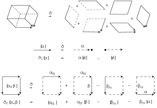
So, in low degrees, the formulas take the following form:

References

- [2] S.I. Adyan, Fragments of the word Delta in a braid group, Mat. Zam. Acad. Sci. SSSR 36-1 (1984) 25–34; translated Math. Notes of the Acad. Sci. USSR; 36-1 (1984) 505–510.
- [3] J. Altobelli & R. Charney, A geometric Rational form for Artin groups of FC type, Geometriae Dedicata; 79; 2000; 277-289.
- [4] V.I. Arnold, The cohomology ring of the colored braid group, Mat. Zametki 5 (1969) 227–231.
- [5] V.I. Arnold, Toplogical invariants of algebraic functions II, Funkt. Anal. Appl. 4 (1970) 91–98.
- [6] J. Birman, K.H. Ko & S.J. Lee, A new approach to the word problem in the braid groups, Advances in Math. 139-2 (1998) 322-353.
- [7] E. Brieskorn, Sur les groupes de tresses (d’après V.I. Arnold), Sém. Bourbaki, exp. 401 (1971), Springer Lect. Notes Math. 317 (1973) 21–44.
- [8] E. Brieskorn & K. Saito, Artin-Gruppen und Coxeter-Gruppen, Invent. Math. 17 (1972) 245–271.
- [9] K.S. Brown, Cohomology of groups, Springer (1982).
- [10] H. Cartan & S. Eilenberg, Hmological Algebra, Princeton University Press, Princeton (1956).
- [11] R. Charney, Artin groups of finite type are biautomatic, Math. Ann. 292-4 (1992) 671–683.
- [12] R. Charney, Geodesic automation and growth functions for Artin groups of finite type, Math. Ann. 301-2 (1995) 307–324.
- [13] R. Charney, J. Meier, & K. Whittlesey, Bestvina’s normal form complex and the homology of Garside groups, Preprint.
- [14] F. Cohen, Cohomology of braid spaces, Bull. Amer. Math. Soc. 79 (1973) 763–766.
- [15] F. Cohen, Artin’s braid groups, classical homotopy theory, and sundry other curiosities, Contemp. Math. 78 (1988) 167–206.
- [16] C. de Concini, M. Salvetti, & F. Stumbo, The top-cohomology of Artin groups with coefficients in rank local systems over , Topology Appl. 78-1 (1997) 5–20.
- [17] P. Dehornoy, Deux propriétés des groupes de tresses, C. R. Acad. Sci. Paris 315 (1992) 633–638.
- [18] P. Dehornoy, Gaussian groups are torsion free, J. of Algebra 210 (1998) 291–297.
- [19] P. Dehornoy, Braids and self-distributivity, Progress in Math. vol. 192, Birkhäuser (2000).
- [20] P. Dehornoy, Groupes de Garside, Ann. Sci. Ec. Norm. Sup., to appear.
- [21] P. Dehornoy, Complete group presentations, Preprint (2001).
- [22] P. Dehornoy & L. Paris, Gaussian groups and Garside groups, two generalizations of Artin groups, Proc. London Math. Soc. 79-3 (1999) 569–604.
- [23] P. Deligne, Les immeubles des groupes de tresses généralisés, Invent. Math. 17 (1972) 273–302.
- [24] E. A. Elrifai & H. R. Morton, Algorithms for positive braids, Quart. J. Math. Oxford 45-2 (1994) 479–497.
- [25] D. Epstein & al., Word Processing in Groups, Jones & Bartlett Publ. (1992).
- [26] D.B. Fuks, Cohomology of the braid group mod. 2, Funct. Anal. Appl. 4 (1970) 143–151.
- [27] F. A. Garside, The braid group and other groups, Quart. J. Math. Oxford 20-78 (1969) 235–254.
- [28] V.V. Goryunov, The cohomology of braid groups of series C and D and certain stratifications, Funkt. Anal. i Prilozhen. 12-2 (1978) 76–77.
- [29] Y. Kobayashi, Complete rewriting systems and homology of monoid algebras, J. Pure Appl. Algebra 65 (1990) 263–275.
- [30] Y. Lafont, A new finiteness condition for monoids presented by complete rewriting systems (after Craig C. Squier), J. Pure Appl. Algebra 98 (1995) 229–244.
- [31] Y. Lafont & A. Prouté, Church-Rosser property and homology of monoids, Math. Struct. Comput. Sci 1 (1991) 297–326.
- [32] M. Picantin, Petits groupes gaussiens, Thèse de doctorat, Université de Caen (2000).
- [33] M. Picantin, The center of small Gaussian groups, J. of Algebra, to appear.
- [34] M. Salvetti, The homotopy type of Artin groups, Math. Res. Letters 1 (1994) 565–577.
- [35] H. Sibert, Extraction of roots in Garside groups, Comm. in Algebra; to appear.
- [36] C. Squier, Word problems and a homological finiteness condition for monoids, J. Pure Appl. Algebra 49 (1987) 201–217.
- [37] C. Squier, The homological algebra of Artin groups, Math. Scand. 75 (1995) 5–43.
- [38] C. Squier, A finiteness condition for rewriting systems, revision by F. Otto and Y. Kobayashi, Theoret. Compt. Sci. 131 (1994) 271–294.
- [39] J. Stallings, The cohomology of pregroups, Conference on Group Theory, Lecture Notes in Math. 319 (1973) 169–182.
- [40] W. Thurston, Finite state algorithms for the braid group, Circulated notes (1988).
- [41] F.V. Vainshtein, Cohomologies of braid groups, Functional Anal. Appl. 12 (1978) 135–137.
- [42] V. V. Vershinin, Braid groups and loop spaces, Uspekhi Mat. Nauk 54-2 (1999) 3–84.