Statistical analysis of stochastic resonance with ergodic diffusion noise
Abstract
A subthreshold signal is transmitted through a channel and may be detected when some noise – with known structure and proportional to some level – is added to the data. There is an optimal noise level, called stochastic resonance, that corresponds to the highest Fisher information in the problem of estimation of the signal. As noise we consider an ergodic diffusion process and the asymptotic is considered as time goes to infinity.
We propose consistent estimators of the subthreshold signal and we solve further a problem of hypotheses testing. We also discuss evidence of stochastic resonance for both estimation and hypotheses testing problems via examples.
keywords: stochastic resonance, diffusion processes, unobservable signal detection, maximum a posterior probability.
MSC: 93E10, 62M99.
1 Introduction
The term ‘stochastic resonance’ was introduced in the early ‘80s (see [2] and [17]) in the study of periodic advance of glaciers on Earth. The stochastic resonance is the effect of nonmonotone dependence of the response of a system on the noise when this noise (for instance the temperature) is added to a periodic input signal (see e.g. [8], in which the author explains also differences and similarities with the notion of stochastic filtering). An extensive review on stochastic resonance and its presence in different fields of applications can be found in [7]. Following [5], as stochastic resonance we intend the phenomenon in which the transmission of a signal can be improved (in terms of statistical quantities) by the addition of noise. From the statistical point of view the problem is to estimate a signal transmitted through a channel. This signal has to be detected by a receiver that can reveal signals louder than a threshold . If is bounded from above by , the signal is not observable and the problem has not a solution. But, if some noise is added to the signal, the perturbed signal may be observable and inference can be done on . Too few noise is not sufficient to give good estimates and too much noise deteriorates excessively the signal. The optimal – in some sense – level of the noise will be called stochastic resonance in this framework. Usually (see [7]) the criterion applied to measure optimality of estimators are the Shannon mutual information or the Kullback divergence. More recently the Fisher information quantity have been also proposed (see [5] and [6]). Here we are concerned with the Fisher information quantity. It happens that this quantity, as a function of the noise, can be maximized for certain noise structures. If there is only one global maximum, the corresponding noise level is the value for which we have stochastic resonance, if several local maxima are present, the phenomenon is called stochastic multi-resonance.
In this paper we study the problem of estimation and hypotheses testing for the following model: we suppose to have a threshold and a subthreshold constant and non negative signal , . We add, in continuous time, a noise that is a trajectory of a diffusion process and we observe the perturbed signal where is the level of the noise. We propose two schemes of observations: i) we observe only the proportion of time spent by the perturbed signal over the threshold and ii) we measure the energy of the perturbed signal when it is above the threshold. The asymptotic is considered as time goes to infinity.
This approach differs from the ones in the current statistical literature basically for two reasons: the noise structure is an ergodic diffusion process and not a sequence of independent and identically distributed random variables and data are collected in continuous time. This second aspect is a substantial difference but it is not a problem from the point of view of applications for the two schemes of observations proposed if one thinks at analogical devices.
We propose two different estimators for the schemes and we study their asymptotic properties. We present an example where, in both cases, it emerges the phenomenon of stochastic resonance. For the same model we also solve the problem of testing the simple hypothesis against the simple alternative by applying the bayesian maximum a posterior probability criterion. It emerges that the overall probability of error is nonmonotonically dependent on . We show again that there exists a non trivial local minimum of this probability that is again the effect of stochastic resonance. The presence of stochastic resonance in this context is noted for the first time here.
The paper is organized as follows. In Section 2 we set up the regularity assumptions of the model. In sections 3 and 4 we prove some asymptotic properties estimators for the two schemes and we calculate numerically the points where the Fisher information quantity attains its maximum for both models. It turns out that the estimators proposed are asymptotically equivalent to the maximum likelihood estimators. Section 5 is devoted to the problem of hypotheses testing. All the figures are collected at the end of the paper.
2 The model and the structure of the noise
Let be the threshold and a constant signal. Taking will not influence the calculations that follows but may improve the exposition, so we use this assumption. Let be a given diffusion process solution to the following stochastic differential equation
| (1) |
with non random initial value . The process is supposed to have the ergodic property with invariant measure and invariant distribution function as . The functions and satisfy the global Lipschitz condition
| (C1) |
where is the Lipschitz constant. Under condition C1, equation (1) has a unique strong solution (see e.g. [13]) but any equivalent condition to C1 can be assumed because we do not use explicitly it in the sequel. The following conditions are needed to ensure the ergodicity of the process . If
| (C2) |
and
| (C3) |
then there exists the stationary distribution function and it takes the following form
Again, any other couple of conditions that imply the existence of can be used instead of C3 and C3.
We perturb the signal by adding, proportionally to some level , the trajectory diffusion process into the channel. The result will be the perturbed signal . This new signal will be detectable only when it is above the threshold . Moreover, is still ergodic with trend and diffusion coefficients respectively and and initial value , but we will not use directly this process. We denote by the observable part of the trajectory of , being the indicator function of the set .
We consider two possibile schemes of observation:
- i)
we observe only the proportion of time spent by over the threshold
- ii)
we measure the energy of the signal
In the next sections, for the two models we establish asymptotic properties of estimators given by the generalized method of moments. In [11] different properties of the generalized method of moments for ergodic diffusion processes are studied. In this note we follows the lines given in the paper of[6] for the i.i.d. setting. These results are interesting in themselves independently from the problem of stochastic resonance. We give an example of stochastic resonance based on the Ornstein-Uhlenbeck process where the phenomenon of stochastic resonance appears pronounced and in which results in a closed form can be written down.
3 Observing the time spent by the process over the threshold
The random variable can be rewritten in terms of the process as
By the ergodic property of we have that
| (2) |
where has as distribution function. From (2) it derives that
so that is a one-to-one continuous function of . From the Glivenko-Cantelli theorem (see e.g. [11]) for the empirical distribution function (EDF) defined by
follows directly that is a -consistent estimator of thus also
is a -consistent estimator for . We can calculate the asymptotic variance of this estimator. It is known that (see [9] and [16]) the EDF is asymptotically Gaussian and in particular
where is the inverse of the analogue of the Fisher information quantity in the problem of distribution function estimation :
| (3) |
where and . The quantity is also the minimax asymptotic lower bound for the quadratic risk associated to the estimation of , so that is asymptotically efficient in this sense.
The asymptotic variance of can be derived by means of the so-called -method (see e.g. [1]):
thus
where is the density of . The quantity can also be derived from the asymptotic minimal variance of the EDF estimator. In fact, with little abuse of notation, by putting and we have that
3.1 Link with the likelihood estimator
We now show that also maximizes the approximate likelihood of the model. In fact, for the central limit theorem for the EDF we have
where is a standard Gaussian random variable. Thus
where is the distribution function of . We approximate the likelihood function of by
that is maximal when
thus, the maximum likelihood estimator of (constructed on the approximated likelihood) reads
So if the approximation above is acceptable, one can infer the optimality property of of having minimum variance from being also the maximum likelihood estimator.
3.2 An example of stochastic resonance
To view the effect of stochastic resonance on the Fisher information we consider a particular example. By setting and the noise become a standard Ornstein-Uhlenbeck process solution to the stochastic differential equation
In such a case, the ergodic distribution function is the Gaussian law with zero mean and variance 1/2. The asymptotic variance assumes the following form
where is the classical error function.
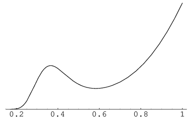
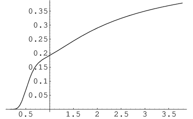
In Figure 1 it is shown that for this model there exists the phenomenon of stochastic resonance. For a fixed level of noise the Fisher information increases as the signal is closer to the threshold . For a fixed value of the signal , the Fisher information, as a function of , has a single maximum, that is the optimal level of noise. For example, if then the optimal level is and for it is .
4 Measuring the observed energy
Suppose that it is possibile to observe not only the time when the perturbed process is over the threshold but also its trajectory above , say , . We now show how it is possibile to estimate the unknown signal from the equivalent of the energy of the signal for : literally from the quantity
We use the following general result from [10] on the estimation of functionals of the invariant distribution functions for ergodic diffusion processes. Let and be such that . Then
is a -consistent estimator for where is distributed according to . In our case and . The estimator can be rewritten as
and it converges to the quantity
that is a continuous and increasing function of , . Its inverse allows us to have again . By applying the -method once again, we can obtain the asymptotic variance of from the asymptotic variance of .
where
The asymptotic variance of is given by (see [10])
where
and its inverse is also the minimal asymptotic variance in the problem of estimation of functionals for ergodic diffusion. Thus, the asymptotic variance of is given by
Remark: By the asymptotic normality of follows that is also the value that maximizes the approximate likelihood function. In fact, as in the previous example, if we approximate the density function of with
it is clear that is its maximum.
4.1 The effect of stochastic resonance
As before, we put in evidence the phenomenon of stochastic resonance by using the Ornstein-Uhlenbeck process as noise. The quantities involved ( and ) transform into the following
(from which it appears that is an increasing function of ) and
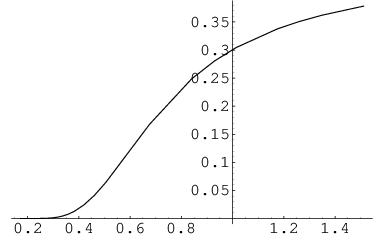
In Figure 1 it is plotted the Fisher information of the model as a function of and . Also in this case there is evidence of stochastic resonance. For a fixed value of is then possibile to find the optimal noise level . For example, taking then we have stochastic resonance at and for , .
5 Hypotheses testing problem
We now study a problem of testing two simple hypotheses for the model discussed in the previous section. As in [4], we apply the maximum a posteriori probability (MAP) criterion. We will see that the decision rules for our model are similar to the one proposed by Chapeau-Blondeau in the i.i.d. setting.
Given the observation we want to verify the null hypothesis that the unknown constant signal is against the simple alternative , with :
Suppose that, before observing , we have a prior information on the parameter, that is and . The MAP criterion uses the following likelihood ratio
and the decision rule is to accept whenever (decision ) or refuse it otherwise (decision ). The overall probability of error is
Let now be
| (4) |
Then, the likelihood appears as
To write explicitly the decision rule and then study the effect of stochastic resonance we have to distinguish three cases: , and .
- 1.
Let it be , then put
Then, if accept and . If , then if reject otherwise accept it. In both cases
- 2.
Let it be , then put
Then, if reject and . If , then if accept otherwise reject it. In both cases
(5) - 3.
Let it be , then put
Then, if reject otherwise accept it. In both cases
5.1 Example
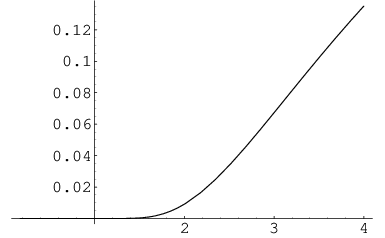
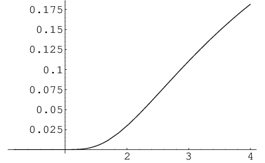
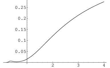
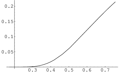
As before, we apply this method to the Ornstein-Uhlenbeck model. In this case the variance , for a fixed threshold and noise level , is a non decreasing function of being only a scale factor (Figure 2 gives a numerical representation of this statement). Thus, the is, in general, given by formula (5). What is amazing is the behavior of . In Figure 3 it is reported the graph of as a function of and given and . For around 1/2 the shows the effect of stochastic resonance. So it appears that in some cases the noise level can reduce sensibly the overall probability of making the wrong decision. This kind of behavior is non outlined in the work of [4].
Remark: Following the same scheme, similar results can be obtained for the model ii) when we observe the energy . In this case it is sufficient to replace in (4) the values of and with the quantities
and with in the decision rule.
Final remarks
The use of ergodic diffusions as noise in the problem of stochastic resonance seems quite powerful. Characterizations of classes of ergodic process that enhance the stochastic resonance can be done (see e.g. [6]) but not in a simple way as in the i.i.d. case as calculations are always cumbersome. The problem of a parametric non constant signal can also be treated while the full nonparametric non constant signal requires more attention and will be object for further investigations. For i.i.d. observations, [14] and [15] considered the problem of non parametric estimation for regression models of the form , . Their approach can be applied in this context.
Other criterion of optimality than the Fisher information quantity can be used as it is usually done in information theory (e.g. Shannon mutual information or Kullback divergence).
The analysis of the overall probability of error seems to put in evidence something new with respect to the current literature (see e.g. [4]). It is worth noting that in a recent paper [3] models driven by ergodic diffusions have also been used but the effect of stochastic resonance is not used to estimate parameters.
References
- [1] Barndorff-Nielsen, O., Cox, D.R., Asymptotic techniques for use in statistics. Chapman & Hall, 1989, Bristol.
- [2] Benzi, R., Sutera, A., Vulpiani, A., The mechanism of stochastic resonance. J. Phys. A, v 14, (1981), L453-L458.
- [3] Berglund, N., Gentz, B., A sample-path approach to noise-induced synchronization: Stochastic resonance in a double-well potential. WIAS preprint no. 627, (2000).
- [4] Chapeau-Blondeau, F., Nonlinear test statistic to improve signal detection in non-Gaussian noise. IEEE Sig. Proc. Lett., v 7, n 7, (2000), 205-207.
- [5] Chapeau-Blondeau, F., Rojas-Varela, J., Information-theoretic measures improved by noise in nonlinear systems. Proc. 14th Int. Conf. on Math. Theory of Networks and Systems, Perpignane, France, (2000), 79-82.
- [6] Greenwood, P.E., Ward,L.M., Wefelmeyer, W., Statistical analysis of stochastic resonance in a simple setting. Phys. Rev. E, v 60, n 4, (2000), 4687-4695.
- [7] Gammaitoni, L., Hänggi, P., Jung, P., Marchesoni, F. , Stochastic resonance. Rev. of Modern Phys., 70, (1998), 223-288.
- [8] Klimontovich, Yu.L., What are stochastic filtering and stochastic resonance? Physics-Uspecky, v 42, n 1, (1999), 37-44.
- [9] Kutoyants, Yu.A., Efficiency of the empirical distribution function for ergodic diffusion. Bernoulli, v 3, n 4, (1997a), 445-456.
- [10] Kutoyants, Yu.A., On semiparametric estimation for ergodic diffusion. Proc. A. Razmadze Math. Inst., 115, (1997b), 45-58.
- [11] Kutoyants, Yu.A., Statistical inference for ergodic diffusion processes. Monography to appear (2000).
- [12] Ibragimov, I.A., Khasminskii, R.Z., Statistical estimation (Asymptotic theory). Springer, 1981, New York.
- [13] Liptser, R.S., Shiryayev, A.N., Statistics of random processes, Part. 1. Springer-Verlag, 1977, New York.
- [14] Müller, U. U., Nonparametric regression for threshold data. Canadian J. Statist, 28, (2000), to appear.
- [15] Müller, U. U., Ward, L. M., Stochastic resonance in a statistical model of a time-integrating detector Phys. Rev. E (3), 61, (2000), to appear.
- [16] Negri, I. (1998). Stationary distribution function estimation for ergodic diffusion processes. Statistical inference for stochastic processes, v 1, n 1, 61-84.
- [17] Nicolis, C., Stochastic aspects of climatic transitions—response to a periodic forcing. Tellus, 34, n 1, (1982), 1-9.
Figures
 |
 |

 |
 |
 |
 |
 |
 |