跳到论文正文
W Papers独立论文阅读器 arXiv:math/0110170 论文正文 计算阅读时间 · 0%
引用这篇论文根据当前论文元数据生成,正式投稿前建议核对。


License: Assumed arXiv.org perpetual non-exclusive license
arXiv:math/0110170v2 [math.SG] 13 Mar 2002

Absolutely graded Floer homologies and intersection forms for four-manifolds with boundaryThanks: PSO was supported by NSF grant number DMS 9971950 and a Sloan Research FellowshipThanks: ZSz was supported by NSF grant number DMS 0107792 and a Packard Fellowship

Peter Ozsváth Address: Department of Mathematics, Princeton University, New Jersey 08540
petero@math.princeton.edu
and Zoltán Szabó Address: Department of Mathematics, Princeton University, New Jersey 08540
szabo@math.princeton.edu
Abstract.

In [22], we introduced absolute gradings on the three-manifold invariants developed in [21] and [20]. Coupled with the surgery long exact sequences, we obtain a number of three- and four-dimensional applications of this absolute grading including strengthenings of the “complexity bounds” derived in [20], restrictions on knots whose surgeries give rise to lens spaces, and calculations of H​F+HF^{+} for a variety of three-manifolds. Moreover, we show how the structure of H​F+HF^{+} constrains the exoticness of definite intersection forms for smooth four-manifolds which bound a given three-manifold. In addition to these new applications, the techniques also provide alternate proofs of Donaldson’s diagonalizability theorem and the Thom conjecture for ℂ​ℙ2{\mathbb{CP}}^{2}.

1. Introduction

In [21] and [20], we introduced Floer-homology invariants (H​F^\widehat{HF}, H​F±HF^{\pm}, and H​F∞HF^{\infty}) for oriented three-manifolds equipped with Spinc{\mathrm{Spin}}^{c} structures. In [20], we derived a number of exact sequences relating H​F+HF^{+} (and also H​F^\widehat{HF}) for three-manifolds which differ by surgeries. In [22], we introduced the corresponding four-dimensional theory, where cobordisms WW between three-manifolds induce maps F^{\widehat{F}}, F±F^{\pm}, F∞F^{\infty} between the corresponding Floer homology theories on the boundaries. One by-product of this four-dimensional theory is an absolute rational lift to the relative ℤ\mathbb{Z} grading on the homology groups for a three-manifold YY endowed with a torsion Spinc{\mathrm{Spin}}^{c} structure (i.e. one whose first Chern class is a torsion element of H2​(Y,ℤ)H^{2}(Y;\mathbb{Z})).

The present article presents a number of three- and four-dimensional applications of the interplay between the absolute gradings and the surgery exact sequences.

1.1. The correction term d⁡(Y)d(Y)

After two introductory sections (Section 2 where we review some of the terminology from the earlier articles, and Section 3, where we pin down the relationship between the absolute gradings and the exact sequence), we give the first application of the absolute gradings: a “correction term” for three-manifolds. For simplicity, we presently assume that YY is a rational homology three-sphere, equipped with a Spinc{\mathrm{Spin}}^{c} structure 𝔱\mathfrak{t}. With the help of the absolute grading, we define a numerical invariant d⁡(Y,𝔱)d(Y,\mathfrak{t}) for YY, which is the minimal degree of any non-torsion class in H​F+​(Y,𝔱)HF^{+}(Y,\mathfrak{t}) coming from H​F∞​(Y,𝔱)HF^{\infty}(Y,\mathfrak{t}). This invariant is analogous to a gauge-theoretic invariant of Frøyshov (see [12]).

The basic properties of dd are conveniently stated with the help of a result which we state after introducing some terminology.

Definition 1.1.

The three-dimensional Spinc{\mathrm{Spin}}^{c} homology bordism group θc\theta^{c} is the set of equivalence classes of pairs (Y,𝔱)(Y,\mathfrak{t}) where YY is a rational homology three-sphere, and 𝔱\mathfrak{t} is a Spinc{\mathrm{Spin}}^{c} structure over YY, and the equivalence relation identifies (Y1,𝔱1)∼(Y2,𝔱2)(Y_{1},\mathfrak{t}_{1})\sim(Y_{2},\mathfrak{t}_{2}) if there is a (connected, oriented, smooth) cobordism WW from Y1Y_{1} to Y2Y_{2} with Hi​(W,ℚ)=0H_{i}(W,\mathbb{Q})=0 for i=1i=1 and 22, which can be endowed with a Spinc{\mathrm{Spin}}^{c} structure 𝔰\mathfrak{s} whose restrictions to Y1Y_{1} and Y2Y_{2} are 𝔱1\mathfrak{t}_{1} and 𝔱2\mathfrak{t}_{2} respectively. The connected sum operation endows this set with the structure of an Abelian group (whose unit is S3S^{3} endowed with its unique Spinc{\mathrm{Spin}}^{c} structure).

There is a classical homomorphism

ρ:θc⟶ℚ/ℤ\rho\colon\theta^{c}\longrightarrow\mathbb{Q}/\mathbb{Z}

(see for instance [1]), defined as follows. Consider a rational homology three-sphere (Y,𝔱)(Y,\mathfrak{t}), and let XX be any four-manifold equipped with a Spinc{\mathrm{Spin}}^{c} structure 𝔰\mathfrak{s} with ∂X≅Y\partial X\cong Y and 𝔰|∂X≅𝔱\mathfrak{s}|\partial X\cong\mathfrak{t}. Then

ρ⁡(Y,𝔱)≡c1​(𝔰)2−sgn⁡(X)4(mod2​ℤ)\rho(Y,\mathfrak{t})\equiv\frac{c_{1}(\mathfrak{s})^{2}-\mathrm{sgn}(X)}{4}\pmod{2\mathbb{Z}}

where sgn⁡(X)\mathrm{sgn}(X) denotes the signature of the intersection form of XX.

Theorem 1.2.

The numerical invariant d⁡(Y,𝔱)d(Y,\mathfrak{t}) descends to give a group homomorphism

d:θc⟶ℚd\colon\theta^{c}\longrightarrow\mathbb{Q}

which is a lift of ρ\rho. Moreover, dd is invariant under conjugation; i.e. d⁡(Y,𝔱)=d⁡(Y,𝔱¯)d(Y,\mathfrak{t})=d(Y,{\overline{\mathfrak{t}}}).

Additivity of the correction term under connected sums, and its behaviour under orientation reversal, is established Section 4. Its rational homology cobordism invariance is established only after more of the four-dimensional theory is developed in Section 9. When b1​(Y)>0b_{1}(Y)>0, torsion Spinc{\mathrm{Spin}}^{c} structures can be endowed with a collection of correction terms. In Subsection 4.2, we discuss this construction in the case where H1​(Y,ℤ)≅ℤH_{1}(Y;\mathbb{Z})\cong\mathbb{Z}.

1.2. Regularized Euler characteristics

When YY is an integral homology three-sphere, H​F+​(Y)HF^{+}(Y) is infinitely generated. (We drop the Spinc{\mathrm{Spin}}^{c} structure from the notation, since it is unique.) To obtain a finitely generated group, we must pass to the quotient

H​Fred+​(Y)=H​F+​(Y)/H​F∞​(Y).HF^{+}_{\mathrm{red}}(Y)=HF^{+}(Y)/HF^{\infty}(Y).

We have the following relationship between the Euler characteristic of H​Fred+​(Y)HF^{+}_{\mathrm{red}}(Y), the correction term for YY, and Casson’s invariant λ⁡(Y)\lambda(Y),

Theorem 1.3.

Let YY be an integer homology three-sphere. Then, the following relationship holds between Casson’s invariant, the Euler characteristic of H​F+HF^{+} (thought of as a ℤ\mathbb{Z}-module), and the correction term:

λ⁡(Y)=χ⁡(H​Fred+​(Y))−12​d​(Y),\lambda(Y)=\chi(HF^{+}_{\mathrm{red}}(Y))-\frac{1}{2}d(Y),

where here Casson’s invariant is normalized so that, if Σ⁡(2,3,5)\Sigma(2,3,5) denotes the Poincaré homology sphere, oriented as the boundary of the negative-definite E​8E8 plumbing, then λ⁡(Σ⁡(2,3,5))=−1\lambda(\Sigma(2,3,5))=-1.

1.3. Invisible three-manifolds.

When YY is an integer homology three-sphere, we define its complexity N⁡(Y)N(Y) to be the rank of H​Fred​(Y)HF_{\rm red}(Y). Let K⊂YK\subset Y be a knot in YY, rr be a rational number, and let Yr​(K)Y_{r}(K) be the integer homology three-sphere obtained by rr surgery on YY along KK. In Theorem  of [20], we gave lower bounds on the sum of complexities of YY and Y1/n​(K)Y_{1/n}(K) (where nn is a whole number), in terms of the Alexander polynomial of KK. Using d⁡(Y)d(Y) in conjunction with N⁡(Y)N(Y), these bounds can be strengthened, according to the following:

Theorem 1.4.

Let YY be an integral homology three-sphere and K⊂YK\subset Y be a knot, whose symmetrized Alexander polynomial is

ΔK​(T)=a0​(K)+∑i=1dai​(K)⋅(Ti+T−i),\Delta_{K}(T)=a_{0}(K)+\sum_{i=1}^{d}a_{i}(K)\cdot(T^{i}+T^{-i}),

then for each positive integer nn, there is a bound

n⁡(|t0​(K)|+2​∑i=1d|ti​(K)|)≤N⁡(Y)+d⁡(Y)2+N⁡(Y1/n​(K))−d​(Y1/n​(K))2,n\left(|t_{0}(K)|+2\sum_{i=1}^{d}|t_{i}(K)|\right)\leq N(Y)+\frac{d(Y)}{2}+N(Y_{1/n}(K))-\frac{d(Y_{1/n}(K))}{2},

where

(1) ti​(K)=∑j=1dj​a|i|+j​(K).t_{i}(K)=\sum_{j=1}^{d}ja_{|i|+j}(K).

An integral homology three-sphere YY for which both N⁡(Y)=0=d⁡(Y)N(Y)=0=d(Y) is called invisible, since these invariants do not distinguish it from S3S^{3}. Of course (in view of Theorem 1.3), all invisible homology three-spheres have λ⁡(Y)=0\lambda(Y)=0. We prove in Section 6 that the set of invisible three-manifolds YY is closed under connected sum and orientation reversal.

Theorem 1.4 has the following immediate consequence:

Corollary 1.5.

If K⊂YK\subset Y is a knot with non-trivial Alexander polynomial in an invisible three-manifold, then any non-trivial surgery on KK gives a three-manifold which is not invisible.

1.4. Surgeries giving lens spaces.

The graded Floer homologies can also be used to place restrictions on knots K⊂S3K\subset S^{3} whose surgeries give lens spaces. For example, we have the following:

Theorem 1.6.

If K⊂S3K\subset S^{3} is a knot with the property that some integral surgery along KK with integral coefficient pp with |p|≤4|p|\leq 4 gives a lens space, then H​F+​(Y0​(K))≅H​F+​(S2×S1)HF^{+}(Y_{0}(K))\cong HF^{+}(S^{2}\times S^{1}). In particular, the Alexander polynomial of KK is trivial.

Remark 1.7.

The “cyclic surgery theorem” of Culler-Gordon-Luecke-Shalen [5] ensures that if KK is not a torus knot, and some surgery along KK gives a lens space, then that surgery is integral. It is conjectured in [14] that the trivial knot is the only knot KK with the property that some surgery on KK gives a lens space L⁡(p,1)L(p,1) with |p|≤4|p|\leq 4.

A +5+5-surgery on the right-handed trefoil gives the lens space −L⁡(5,1)-L(5,1), so care must be taken in generalizing Theorem 1.6. The following result holds for general pp:

Theorem 1.8.

Suppose that K⊂S3K\subset S^{3} is a knot with the property that +p+p surgery on KK gives the lens space L⁡(p,1)L(p,1) (with its canonical orientation). Then, H​F∞​(S03​(K))≅H​F∞​(S2×S1)HF^{\infty}(S^{3}_{0}(K))\cong HF^{\infty}(S^{2}\times S^{1}) as absolutely graded groups; in particular, the Alexander polynomial of KK is trivial.

In fact, Gordon has conjectured (see [13]) that if +p+p surgery on a knot K⊂S3K\subset S^{3} gives L⁡(p,1)L(p,1), then KK is the unknot. Moreover, Berge [3] has conjectured a complete list of knots which give rise to lens spaces.

Theorems 1.6 and 1.8 are proved in Section 7, where they are given as a corollaries to a theorem, Theorem 7.2, which, for any fixed pp and qq, gives strong restrictions on knots K⊂S3K\subset S^{3} for which +p+p surgery gives the lens space L⁡(p,q)L(p,q). Specifically, if KK is such a knot, the theorem shows how H​F+HF^{+} of the zero-surgery (and hence the Alexander polynomial of the knot) is determined, up to a finite indeterminacy, by the correction terms for L⁡(p,q)L(p,q). The indeterminacy comes from certain allowed permutations of these correction terms. The terms themselves are calculated in Proposition 4.8 (see [24] for a more conceptual interpretation of these numbers). For another illustration of these constraints, we tabulate at the end of this paper (c.f Subsection 10.3) the possible Alexander polynomials of knots in S3S^{3} for which some positive integral surgery p≤26p\leq 26 gives a lens space.

Turned around, Theorem 7.2 also gives obstructions to realizing lens spaces as integral surgeries on a knot in the three-sphere. For example, these techniques show that the lens space L⁡(22,3)L(22,3) – and indeed, any lens spaces in the family L⁡(2​k​(3+8​k),2​k+1)L(2k(3+8k),2k+1) where kk is any positive integer not divisible by 44 – is not obtained by integral surgery on a single knot K⊂S3K\subset S^{3}. This obstruction is “S3S^{3}-specific”. An argument of Fintushel and Stern gives a necessary and sufficient condition for L⁡(p,q)L(p,q) to be realized as integral surgery on a knot in a homology sphere: the condition is that ±q\pm q be a square modulo pp, a condition which all the lens spaces in this family satisfy. (This application is described in Proposition 7.9.)

1.5. Some calculations.

We give several calculations of N⁡(Y)N(Y) and d⁡(Y)d(Y), including calculations of both invariants for integer homology spheres obtained as surgeries on the (p,q)(p,q) torus knot. Indeed, we calculate all of H​F+HF^{+} for the Brieskorn spheres Σ⁡(2,3,6​n±1)\Sigma(2,3,6n\pm 1). Moreover, we calculate H​F+​(En)HF^{+}(E_{n}) where EnE_{n} is the three-manifold obtained by 1/n1/n surgery with n>0n>0 on the figure eight knot in S3S^{3} (c.f. Proposition 8.3):

H​Fk+​(En)≅{ℤif k≡0(mod2) and k≥0ℤnif k=−10otherwise.HF^{+}_{k}(E_{n})\cong\left\{\begin{array}[]{ll}\mathbb{Z}&{\text{if $k\equiv 0\pmod{2}$ and $k\geq 0$}}\\ \mathbb{Z}^{n}&{\text{if $k=-1$}}\\ 0&{\text{otherwise}}\end{array}\right..

We also give the following simple calculation for the invariants of T3T^{3}:

Proposition 1.9.

Let T3T^{3} denote the three-dimensional torus. Then, we have H1​(T3,ℤ)H_{1}(T^{3};\mathbb{Z})-module isomorphisms:

H​F^​(T3)\displaystyle\widehat{HF}(T^{3}) ≅\displaystyle\cong H2​(T3,ℤ)⊕H1​(T3,ℤ),\displaystyle H^{2}(T^{3};\mathbb{Z})\oplus H^{1}(T^{3};\mathbb{Z}),
H​F+​(T3)\displaystyle HF^{+}(T^{3}) ≅\displaystyle\cong (H2​(T3,ℤ)⊕H1​(T3,ℤ))⊗ℤℤ⁡[U−1],\displaystyle\Big(H^{2}(T^{3};\mathbb{Z})\oplus H^{1}(T^{3};\mathbb{Z})\Big)\otimes_{\mathbb{Z}}\mathbb{Z}[U^{-1}],
H​F∞​(T3)\displaystyle HF^{\infty}(T^{3}) ≅\displaystyle\cong (H2​(T3,ℤ)⊕H1​(T3,ℤ))⊗ℤℤ⁡[U,U−1].\displaystyle\Big(H^{2}(T^{3};\mathbb{Z})\oplus H^{1}(T^{3};\mathbb{Z})\Big)\otimes_{\mathbb{Z}}\mathbb{Z}[U,U^{-1}].

The absolute grading is symmetric, in the sense that gr~​(H2​(T3,ℤ)⊂H​F^​(T3))=1/2\widetilde{\mathrm{gr}}(H^{2}(T^{3};\mathbb{Z})\subset\widehat{HF}(T^{3}))=1/2, gr~(H1(T3;ℤ)⊂H​F^(T3))=−1/2\widetilde{\mathrm{gr}}(H^{1}(T^{3};\mathbb{Z})\subset\widehat{HF}(T^{3}))=-1/2.

Further calculations are given for surgeries on certain pretzel knots, via surgery long exact sequences which mirror the skein relations for calculating Alexander polynomials.

1.6. Intersection forms of definite four-manifolds.

By analyzing the maps FW,𝔰∞F^{\infty}_{W,\mathfrak{s}} for negative-definite cobordisms, we give an alternative proof of Donaldson’s diagonalizability theorem:

Theorem 1.10.

(Donaldson) If XX is a smooth, closed, oriented four-manifold with definite intersection form, then the form of XX is diagonalizable over ℤ\mathbb{Z}.

Indeed, applying the same idea to four-manifolds which bound a given integer homology three-sphere YY, we obtain the following analogue of a theorem of Frøyshov.

Let YY be an integral homology three-sphere, and XX be a four-manifold which bounds YY. There is an intersection form

QX:(H2​(X,ℤ)/Tors)⊗(H2​(X,ℤ)/Tors)⟶ℤ.Q_{X}\colon(H_{2}(X;\mathbb{Z})/\mathrm{Tors})\otimes(H_{2}(X;\mathbb{Z})/\mathrm{Tors})\longrightarrow\mathbb{Z}.

A characteristic vector for this intersection form is an element ξ∈H2​(X,ℤ)/Tors\xi\in H_{2}(X;\mathbb{Z})/\mathrm{Tors} with

ξ⋅v≡v⋅v(mod2)\xi\cdot v\equiv v\cdot v\pmod{2}

for each v∈H2​(X,ℤ)/Torsv\in H_{2}(X;\mathbb{Z})/\mathrm{Tors}. (We write ξ⋅η\xi\cdot\eta for QX​(ξ,η)Q_{X}(\xi,\eta), and ξ2\xi^{2} for QX​(ξ,ξ)Q_{X}(\xi,\xi).)

Theorem 1.11.

Let YY be an integral homology three-sphere, then for each negative-definite four-manifold XX which bounds YY, we have the inequality:

ξ2+rk⁡(H2​(X,ℤ))≤4​d​(Y),\xi^{2}+\mathrm{rk}(H^{2}(X;\mathbb{Z}))\leq 4d(Y),

for each characteristic vector ξ\xi.

This theorem has an obvious generalization to rational homology three-spheres, and, indeed, generalizations for three-manifolds with b1​(Y)>0b_{1}(Y)>0 discussed in Section 9.3. When H1​(Y,ℤ)≅ℤH_{1}(Y;\mathbb{Z})\cong\mathbb{Z}, the inequality can be used as obstruction to realizing YY as the boundary of an integral homology S2×D2S^{2}\times D^{2}. Moreover, when applied to certain circle bundles over two-manifolds, the intersection form bounds provide another proof of the Thom conjecture for ℂ​ℙ2{\mathbb{CP}}^{2} first proved by Kronheimer-Mrowka [16] and Morgan-Szabó-Taubes [19], c.f. Subsection 9.4. The proof given here is analogous to a Seiberg-Witten proof given recently by Strle, see [25].

In Section 10, we close with some other applications of the intersection form bounds, as combined with the calculations from Section 8. Specifically, we show how the results constrain the intersection forms of four-manifolds which bound certain Seifert fibered spaces. In particular, in Subsection 10.2, we exhibit a three-manifold whose first homology is isomorphic to ℤ\mathbb{Z} and which can be expressed as surgery on a certain two-component link in S3S^{3}, but which cannot be expressed as surgery on a single knot. Finally, we close with a table of allowed Alexander polynomials of knots giving rise to (small) lens spaces.

Acknowledgements: It is our pleasure to thank Cameron Gordon, Robion Kirby, Tomasz Mrowka, and András Stipsicz for their encouragement during the preparation of this work. We would especially like to thank Cameron Gordon for some very useful suggestions on an early version of this paper.

2. Floer homologies and maps between them

In [22], we showed how the constructions from [21] and [20] can give rise to a naturally associated assignment which associates to a three-manifold YY equipped with a Spinc{\mathrm{Spin}}^{c} structure 𝔱\mathfrak{t}, four relatively ℤ/c1​(𝔱)∪H1​(Y,ℤ)​ℤ\mathbb{Z}/{c_{1}(\mathfrak{t})\cup H^{1}(Y;\mathbb{Z})}\mathbb{Z}-graded Abelian groups H​F^\widehat{HF}, H​F+HF^{+}, H​F−HF^{-}, and H​F∞HF^{\infty}, the latter three of which are also endowed with the action by a polynomial algebra ℤ⁡[U]\mathbb{Z}[U], where multiplication by UU lowers relative degree by 22. All four groups are acted upon by the exterior algebra Λ∗​H1​(Y,ℤ)/Tors\Lambda^{*}H_{1}(Y;\mathbb{Z})/\mathrm{Tors}.

In fact, these groups are related by functorially associated long exact sequences:

(2) ...→H​F^​(Y,𝔱)→ι^H​F+​(Y,𝔱)→UH​F+​(Y,𝔱)→...\begin{CD}...@>{}>{}>\widehat{HF}(Y,\mathfrak{t})@>{\widehat{\iota}}>{}>HF^{+}(Y,\mathfrak{t})@>{U}>{}>HF^{+}(Y,\mathfrak{t})@>{}>{}>...\end{CD}

and

(3) ...→H​F−​(Y,𝔱)→ιH​F∞​(Y,𝔱)→πH​F+​(Y,𝔱)→...\begin{CD}...@>{}>{}>HF^{-}(Y,\mathfrak{t})@>{\iota}>{}>HF^{\infty}(Y,\mathfrak{t})@>{\pi}>{}>HF^{+}(Y,\mathfrak{t})@>{}>{}>...\end{CD}

The second long exact sequence (which we use more often) will frequently be abbreviated H​F∘​(Y,𝔱)HF^{\circ}(Y,\mathfrak{t}). Note that maps in the first sequence are equivariant under the action of Λ∗​(Y)/Tors\Lambda^{*}(Y)/\mathrm{Tors}, while those for the second are equivariant under the action of ℤ⁡[U]⊗ℤΛ∗​(Y)/Tors\mathbb{Z}[U]\otimes_{\mathbb{Z}}\Lambda^{*}(Y)/\mathrm{Tors}.

When WW is a (smooth) cobordism from a three-manifold Y1Y_{1} to Y2Y_{2}, equipped with a Spinc{\mathrm{Spin}}^{c} structure 𝔰\mathfrak{s} whose restrictions to the two boundary components are 𝔱1\mathfrak{t}_{1} and 𝔱2\mathfrak{t}_{2} respectively, then there are induced maps between the long exact sequences:

...→H​F−​(Y1,𝔱1)→ιH​F∞​(Y1,𝔱1)→πH​F+​(Y1,𝔱1)→...FW,𝔰−↓FW,𝔰∞↓FW,𝔰+↓...→H​F−​(Y2,𝔱2)→ιH​F∞​(Y2,𝔱2)→πH​F+​(Y2,𝔱2)→...\begin{CD}...@>{}>{}>HF^{-}(Y_{1},\mathfrak{t}_{1})@>{\iota}>{}>HF^{\infty}(Y_{1},\mathfrak{t}_{1})@>{\pi}>{}>HF^{+}(Y_{1},\mathfrak{t}_{1})@>{}>{}>...\\ &&@V{F^{-}_{W,\mathfrak{s}}}V{}V@V{F^{\infty}_{W,\mathfrak{s}}}V{}V@V{F^{+}_{W,\mathfrak{s}}}V{}V\\ ...@>{}>{}>HF^{-}(Y_{2},\mathfrak{t}_{2})@>{\iota}>{}>HF^{\infty}(Y_{2},\mathfrak{t}_{2})@>{\pi}>{}>HF^{+}(Y_{2},\mathfrak{t}_{2})@>{}>{}>...\\ \end{CD}

and

...→H​F^​(Y1,𝔱1)→ι^H​F+​(Y1,𝔱1)→UH​F+​(Y1,𝔱1)→...F^W,𝔰↓FW,𝔰+↓FW,𝔰+↓...→H​F^​(Y2,𝔱2)→ι^H​F+​(Y2,𝔱2)→UH​F+​(Y2,𝔱2)→...\begin{CD}...@>{}>{}>\widehat{HF}(Y_{1},\mathfrak{t}_{1})@>{\widehat{\iota}}>{}>HF^{+}(Y_{1},\mathfrak{t}_{1})@>{U}>{}>HF^{+}(Y_{1},\mathfrak{t}_{1})@>{}>{}>...\\ &&@V{{\widehat{F}}_{W,\mathfrak{s}}}V{}V@V{F^{+}_{W,\mathfrak{s}}}V{}V@V{F^{+}_{W,\mathfrak{s}}}V{}V\\ ...@>{}>{}>\widehat{HF}(Y_{2},\mathfrak{t}_{2})@>{\widehat{\iota}}>{}>HF^{+}(Y_{2},\mathfrak{t}_{2})@>{U}>{}>HF^{+}(Y_{2},\mathfrak{t}_{2})@>{}>{}>...\\ \end{CD}

The maps F^W,𝔰{\widehat{F}}_{W,\mathfrak{s}}, FW,𝔰±F^{\pm}_{W,\mathfrak{s}}, and FW,𝔰∞F^{\infty}_{W,\mathfrak{s}} are uniquely defined up to multiplication by an overall sign ±1\pm 1.

These maps also admit an action by Λ∗​H1​(W)/Tors\Lambda^{*}H_{1}(W)/\mathrm{Tors}. This action is related to the analogous actions over the three-manifolds, according to the following formula. Fix arbitrary elements γi∈H1​(Yi)/Tors\gamma_{i}\in H_{1}(Y_{i})/\mathrm{Tors} for i=1,2i=1,2, and let γ∈H1​(W)/Tors\gamma\in H_{1}(W)/\mathrm{Tors} be the homology class obtained as γ=j1​(γ1)−j2​(γ2)\gamma=j_{1}(\gamma_{1})-j_{2}(\gamma_{2}), where for i=1,2i=1,2, jij_{i} denotes the natural inclusion ji:H1​(Yi)⟶H1​(X)j_{i}\colon H_{1}(Y_{i})\longrightarrow H_{1}(X). Then,

±(γ⊗FW,𝔰)​(ξ)=FW,𝔰​(γ1⋅ξ)−γ2⋅FW,𝔰​(ξ).\pm(\gamma\otimes F_{W,\mathfrak{s}})(\xi)=F_{W,\mathfrak{s}}(\gamma_{1}\cdot\xi)-\gamma_{2}\cdot F_{W,\mathfrak{s}}(\xi).

In particular, if γ1\gamma_{1} and γ2\gamma_{2} are homologous in WW, then

FW,𝔰​(γ1⋅ξ)=γ2⋅FW,𝔰​(ξ).F_{W,\mathfrak{s}}(\gamma_{1}\cdot\xi)=\gamma_{2}\cdot F_{W,\mathfrak{s}}(\xi).

Suppose now that YY is equipped with a torsion Spinc{\mathrm{Spin}}^{c} structure. In Theorem  of [22], we showed that H​F∘​(Y,𝔱)HF^{\circ}(Y,\mathfrak{t}), and also H​F^​(Y,𝔱)\widehat{HF}(Y,\mathfrak{t}) can be given an absolute ℚ\mathbb{Q} grading gr~\widetilde{\mathrm{gr}} which lifts the relative ℤ\mathbb{Z} grading. It is uniquely characterized by the following properties:

  • •

    ι^{\widehat{\iota}}, ι\iota, and π\pi above preserve the absolute grading

  • •

    H​F^​(S3)\widehat{HF}(S^{3}) is supported in absolute grading zero

  • •

    if WW is a cobordism from Y1Y_{1} to Y2Y_{2}, and ξ∈H​F∞​(Y1,𝔱1)\xi\in HF^{\infty}(Y_{1},\mathfrak{t}_{1}), then

    (4) gr~​(FW,𝔰​(ξ))−gr~​(ξ)=c1​(𝔰)2−2​χ​(W)−3​σ​(W)4,\widetilde{\mathrm{gr}}(F_{W,\mathfrak{s}}(\xi))-\widetilde{\mathrm{gr}}(\xi)=\frac{c_{1}(\mathfrak{s})^{2}-2\chi(W)-3\sigma(W)}{4},

    where 𝔱i=𝔰|Yi\mathfrak{t}_{i}=\mathfrak{s}|Y_{i} for i=1,2i=1,2.

The existence and characterization of this absolute grading is the key result we use here from [22].

3. Exact sequences and absolute gradings

Recall that in [20], surgery long exact sequences for H​F+HF^{+} and H​F^\widehat{HF} were established. We give now a graded refinement, focusing mainly on the case of H​F+HF^{+}. The key point is the relationship between the maps in the long exact sequences and the maps induced by the cobordisms obtained by surgeries on knots.

More concretely, recall that when KK is a knot in an integral homology three-sphere, Theorem  of [20] gives a long exact sequence

...→H​F+​(Y)→F1H​F+​(Y0)→F2H​F+​(Y1)→F3H​F+​(Y)→...,\begin{CD}...@>{}>{}>HF^{+}(Y)@>{F_{1}}>{}>HF^{+}(Y_{0})@>{F_{2}}>{}>HF^{+}(Y_{1})@>{F_{3}}>{}>HF^{+}(Y)@>{}>{}>...,\end{CD}

where Y0=Y0​(K)Y_{0}=Y_{0}(K) and Y1=Y1​(K)Y_{1}=Y_{1}(K) are the three-manifolds obtained by 00-surgery and +1+1-surgery on YY along KK (using its canonical framing). Here,

H​F+​(Y0)=⨁𝔱∈Spinc​(Y0)H​F+​(Y0,𝔱).HF^{+}(Y_{0})=\bigoplus_{\mathfrak{t}\in{\mathrm{Spin}}^{c}(Y_{0})}HF^{+}(Y_{0},\mathfrak{t}).

The maps F1F_{1} and F2F_{2} were defined by counting pseudo-holomorphic triangles in a Heegaard triple. An easy comparison between the definition of the maps in [20] and the maps associated to two-handles (Subsection  of [21]) shows that F1F_{1} and F2F_{2} are sums of maps associated to cobordisms; i.e.

F1=∑𝔰∈W0±FW0,𝔰,\displaystyle F_{1}=\sum_{\mathfrak{s}\in W_{0}}\pm F_{W_{0},\mathfrak{s}}, and F2=∑𝔰∈W1±FW1,𝔰,\displaystyle F_{2}=\sum_{\mathfrak{s}\in W_{1}}\pm F_{W_{1},\mathfrak{s}},

where W0W_{0} is the cobordism from YY to Y0Y_{0} defined by attaching a single two-handle to YY (with 00-framing), and W1W_{1} is the cobordism from Y0Y_{0} to Y1Y_{1} defined by attaching a single two-handle to Y0Y_{0}. (The signs are chosen as in the proof of Theorem  of [20] to make the sequence exact.) Observe that Spinc{\mathrm{Spin}}^{c} structures on both W0W_{0} and W1W_{1} are uniquely determined by their restrictions to Y0Y_{0}.

Note that the map F3F_{3} arises as the coboundary map of an associated long exact sequence, though one could alternatively realize it, too, as a sum of maps belonging to cobordisms (compare [4]). However, for our present purposes, it suffices to understand properties of the maps F1F_{1} and F2F_{2}.

Lemma 3.1.

Let K⊂YK\subset Y be a knot in an integral homology three-sphere, and let 𝔱0\mathfrak{t}_{0} denote the Spinc{\mathrm{Spin}}^{c} structure over Y0Y_{0} with trivial first Chern class. In the exact sequence

...→H​F+​(Y)→F1H​F+​(Y0)→F2H​F+​(Y1)→F3H​F+​(Y)→...,\begin{CD}...@>{}>{}>HF^{+}(Y)@>{F_{1}}>{}>HF^{+}(Y_{0})@>{F_{2}}>{}>HF^{+}(Y_{1})@>{F_{3}}>{}>HF^{+}(Y)@>{}>{}>...,\end{CD}

the component of F1F_{1} mapping into H​F+​(Y0,𝔱0)HF^{+}(Y_{0},\mathfrak{t}_{0}) (now thought of as absolutely ℚ\mathbb{Q}-graded) has degree −1/2-1/2, the restriction of F2F_{2} to H​F+​(Y0,𝔱0)HF^{+}(Y_{0},\mathfrak{t}_{0}) has degree −1/2-1/2.

Proof. In view of the above remarks, the component of F1F_{1} landing in the H​F+​(Y0,𝔱0)HF^{+}(Y_{0},\mathfrak{t}_{0}) summand is the map induced by the cobordism W0W_{0}, endowed with the Spinc{\mathrm{Spin}}^{c} structure 𝔰0\mathfrak{s}_{0} with trivial first Chern class. This cobordism is obtained by a single one-handle addition (so its χ=0\chi=0), and its signature σ=0\sigma=0. Thus, by Equation (4), the result follows. The map F2F_{2} is also obtained by a single two-handle addition, with signature zero.           

Remark 3.2.

Note that the above discussion could have been made using H​F^\widehat{HF} in place of H​F+HF^{+}, with only notational changes.

When YY is an integral homology three-sphere, we can compare the absolute grading of H​F∘​(Y)HF^{\circ}(Y) as defined in Section  of [22] with the absolute ℤ/2​ℤ\mathbb{Z}/{2}\mathbb{Z} grading as defined in [20].

Observe first that for an integral homology three-sphere, the absolute grading of Section  of [22] is actually a ℤ\mathbb{Z} lift (rather than a ℚ\mathbb{Q} lift) of the usual relative grading. To see this, let WW be a a cobordism containing only two-handles from S3S^{3} to YY (used in the definition of the absolute grading), and observe that

c1​(𝔰)2−2​χ​(W)−3​s​g​n​(W)4≡c1​(𝔰)2−sgn⁡(W)4,(modℤ)\frac{c_{1}(\mathfrak{s})^{2}-2\chi(W)-3\mathrm{sgn}(W)}{4}\equiv\frac{c_{1}(\mathfrak{s})^{2}-\mathrm{sgn}(W)}{4},\pmod{\mathbb{Z}}

(where sgn⁡(W)\mathrm{sgn}(W) is the signature of the intersection form of WW) which is integral since c1​(𝔰)c_{1}(\mathfrak{s}) is a characteristic vector for the definite, unimodular form H2​(W,ℤ)H^{2}(W;\mathbb{Z}).

Next, recall that in general H​F∘​(Y,𝔱)HF^{\circ}(Y,\mathfrak{t}) comes equipped with an absolute ℤ/2​ℤ\mathbb{Z}/{2}\mathbb{Z} grading, defined in Subsection  of [20]. When YY is an integral homology three-sphere, this is the ℤ/2​ℤ\mathbb{Z}/{2}\mathbb{Z} grading characterized by the property that

χ​(H​F^​(Y))=1.\chi(\widehat{HF}(Y))=1.

(Since there is only one Spinc{\mathrm{Spin}}^{c} structure in this case, we drop it from the notation.)

An equivalent (but technically more useful) formulation of this grading follows from the calculation of H​F∞HF^{\infty} of an integer homology three-sphere, Theorem  of [20], where it is shown that H​F∞​(Y)≅ℤ⁡[U,U−1]HF^{\infty}(Y)\cong\mathbb{Z}[U,U^{-1}]. We then define the ℤ/2​ℤ\mathbb{Z}/{2}\mathbb{Z} degree so that H​F∞​(Y)HF^{\infty}(Y) is supported in even degree.

Proposition 3.3.

If YY is an integral homology three-sphere, then the parity of the absolute ℤ\mathbb{Z} grading defined above is the absolute ℤ/2​ℤ\mathbb{Z}/{2}\mathbb{Z} grading defined in [20].

Proof. Both gradings (mod 22) agree on YY, if and only if they agree on Y1Y_{1}. This is easily seen from the long exact sequence connecting H​F+​(Y)HF^{+}(Y), H​F+​(Y0)HF^{+}(Y_{0}), and H​F+​(Y1)HF^{+}(Y_{1}), according to which the composite map from YY to Y1Y_{1} shifts the absolute ℤ\mathbb{Z}-degree by −1-1 (modulo two); it also shifts the absolute ℤ/2​ℤ\mathbb{Z}/{2}\mathbb{Z} degree. The result then follows from the model case S3S^{3}, together with fact that every integer homology can be constructed from S3S^{3} by a sequence of ±1\pm 1 surgeries.           

Another case which will interest us is that of three-manifolds Y0Y_{0} with H1​(Y0,ℤ)≅ℤH_{1}(Y_{0};\mathbb{Z})\cong\mathbb{Z}. For such a manifold, the absolute ℤ/2​ℤ\mathbb{Z}/{2}\mathbb{Z} grading from [20] is defined so that the image of the action by H1​(Y0,ℤ)H_{1}(Y_{0};\mathbb{Z}) on H​F∞​(Y0)HF^{\infty}(Y_{0}) has degree zero modulo 22.

Proposition 3.4.

Let Y0Y_{0} be a three-manifold with H1​(Y0,ℤ)≅ℤH_{1}(Y_{0};\mathbb{Z})\cong\mathbb{Z}, and let 𝔱0\mathfrak{t}_{0} be the Spinc{\mathrm{Spin}}^{c} structure with c1​(𝔱0)=0c_{1}(\mathfrak{t}_{0})=0. Then the parity of gr~+12\widetilde{\mathrm{gr}}+\frac{1}{2} is the absolute ℤ/2​ℤ\mathbb{Z}/{2}\mathbb{Z} grading given above.

Proof. By surgering out the one-dimensional homology, we can fit Y0Y_{0} into a long exact sequence for YY, Y0Y_{0}, and Y1Y_{1}, where YY and Y1Y_{1} are integer homology three-spheres. The result then follows from the grading in the long exact sequence (Lemma 3.1) together with Proposition 3.3 above.           

We now turn to the graded refinement of the long exact sequence, after introducing some notation. Let YY be a closed, oriented three-manifold and a∈ℝa\in\mathbb{R}, and let 𝔰0\mathfrak{s}_{0} be a torsion Spinc{\mathrm{Spin}}^{c} structure. Then, we let

H​F≤a+​(Y,𝔰0)⊂H​F+​(Y,𝔰0)HF^{+}_{\leq a}(Y,\mathfrak{s}_{0})\subset HF^{+}(Y,\mathfrak{s}_{0})

denote the subgroup generated by homogeneous elements ξ\xi with degree gr~​(ξ)≤a\widetilde{\mathrm{gr}}(\xi)\leq a. Let 𝔗⊂Spinc​(Y){\mathfrak{T}}\subset{\mathrm{Spin}}^{c}(Y) denote the subset of torsion Spinc{\mathrm{Spin}}^{c} structures, then

H​F≤a+​(Y)=(⨁𝔰0∈𝔗H​F≤a+​(Y,𝔰0))⊕(⨁𝔱∈Spinc​(Y)−𝔗H​F+​(Y,𝔱)).HF^{+}_{\leq a}(Y)=\left(\bigoplus_{\mathfrak{s}_{0}\in{\mathfrak{T}}}HF^{+}_{\leq a}(Y,\mathfrak{s}_{0})\right)\oplus\left(\bigoplus_{\mathfrak{t}\in{\mathrm{Spin}}^{c}(Y)-{\mathfrak{T}}}HF^{+}(Y,\mathfrak{t})\right).

We have the following:

Theorem 3.5.

Let K⊂YK\subset Y be a knot in an integral homology three-sphere. Then, for all sufficiently large nn, we have an exact sequence

...→H​F≤2​n+1+​(Y)→F1H​F≤2​n+1+​(Y0)→F2H​F≤2​n+1+​(Y1)→F3...\begin{CD}...@>{}>{}>HF^{+}_{\leq 2n+1}(Y)@>{F_{1}}>{}>HF^{+}_{\leq 2n+1}(Y_{0})@>{F_{2}}>{}>HF^{+}_{\leq 2n+1}(Y_{1})@>{F_{3}}>{}>...\end{CD}

Proof. Observe that Ker​F1⊂H​F+​(Y)\mathrm{Ker}F_{1}\subset HF^{+}(Y) is a finitely generated ℤ\mathbb{Z}-module, since for all sufficently large kk, the 𝔰0\mathfrak{s}_{0} component of F1F_{1} carries H​F2​k+​(Y)HF^{+}_{2k}(Y) isomomorphically to H​F2​k−1/2+​(Y0,𝔰0)HF^{+}_{2k-1/2}(Y_{0},\mathfrak{s}_{0}), and H​F2​k+1+​(Y)=0HF^{+}_{2k+1}(Y)=0 (we are using here the H​F∞HF^{\infty} characterization of the ℤ/2​ℤ\mathbb{Z}/{2}\mathbb{Z} grading and Proposition 3.3 to compare it with the absolute ℤ\mathbb{Z} grading). Moreover, this kernel is the image of F3​(H​F+​(Y1))F_{3}(HF^{+}(Y_{1})). It follows that we can find an nn large enough that

F3​(H​F+​(Y1))=F3​(H​F≤2​n+1+​(Y1)).F_{3}(HF^{+}(Y_{1}))=F_{3}(HF^{+}_{\leq 2n+1}(Y_{1})).

Moreover, since ⨁𝔱≠𝔰0H​F+​(Y0,𝔱)\bigoplus_{\mathfrak{t}\neq\mathfrak{s}_{0}}HF^{+}(Y_{0},\mathfrak{t}) is finitely generated, we have that F2F_{2} maps H​F≤2​n+1+​(Y0)HF^{+}_{\leq 2n+1}(Y_{0}) into H​F≤2​n+1+​(Y1)HF^{+}_{\leq 2n+1}(Y_{1}), for all sufficiently large nn.

The theorem then follows from the Lemma 3.1.           

3.1. More exact sequences: fractional surgeries

There are analogues of the refined exact sequence (Theorem 3.5) which holds for fractional surgeries, as well.

Recall that in Theorem  of [20], we established an exact sequence for fractional surgeries of the form

(5) ...→H​F+​(Y)→F~1H​F¯+​(Y0,ℤ/q​ℤ)→F~2H​F+​(Y1/q)→F~3H​F+​(Y)→...,\begin{CD}...@>{}>{}>HF^{+}(Y)@>{{\widetilde{F}}_{1}}>{}>\underline{HF}^{+}(Y_{0};\mathbb{Z}/{q}\mathbb{Z})@>{{\widetilde{F}}_{2}}>{}>HF^{+}(Y_{1/q})@>{{\widetilde{F}}_{3}}>{}>HF^{+}(Y)@>{}>{}>...,\end{CD}

where YY is an integral homology sphere, and qq is any real number. In the above sequence,

H​F¯+​(Y0,ℤ/q​ℤ)=⨁𝔱∈Spinc​(Y0)H​F¯+​(Y0,𝔱,ℤ/q​ℤ)\underline{HF}^{+}(Y_{0};\mathbb{Z}/{q}\mathbb{Z})=\bigoplus_{\mathfrak{t}\in{\mathrm{Spin}}^{c}(Y_{0})}\underline{HF}^{+}(Y_{0},\mathfrak{t};\mathbb{Z}/{q}\mathbb{Z})

is a sum of H​F+HF^{+}-groups twisted by some representation

H1​(Y0,ℤ)⟶ℤ/q​ℤ.H_{1}(Y_{0};\mathbb{Z})\longrightarrow\mathbb{Z}/{q}\mathbb{Z}.

Observe that the 𝔱0\mathfrak{t}_{0}-component of H​F¯+​(Y0,ℤ/q​ℤ)\underline{HF}^{+}(Y_{0},\mathbb{Z}/{q}\mathbb{Z}) (where, as usual, c1​(𝔱0)=0c_{1}(\mathfrak{t}_{0})=0) can be given an absolute ℚ\mathbb{Q}-grading (inherited from the absolute grading of the untwisted group).

Defining H​F¯≤2​n+1+​(Y0,ℤ/q​ℤ)\underline{HF}^{+}_{\leq 2n+1}(Y_{0};\mathbb{Z}/{q}\mathbb{Z}) with respect to this grading on the torsion component, we have the following truncated exact sequence (analogous to Theorem 3.6):

Theorem 3.6.

Let K⊂YK\subset Y be a knot in an integral homology three-sphere. Then, for all sufficiently large nn, there is an exact sequence

...→H​F≤2​n+1+​(Y)→F~1H​F¯≤2​n+1+​(Y0,ℤ/q​ℤ)→F~2H​F≤2​n+1+​(Y1/q)→F~3...\begin{CD}...@>{}>{}>HF^{+}_{\leq 2n+1}(Y)@>{{\widetilde{F}}_{1}}>{}>\underline{HF}^{+}_{\leq 2n+1}(Y_{0},\mathbb{Z}/{q}\mathbb{Z})@>{{\widetilde{F}}_{2}}>{}>HF^{+}_{\leq 2n+1}(Y_{1/q})@>{{\widetilde{F}}_{3}}>{}>...\end{CD}

The proof of the above theorem is complicated by the fact that in the proof of the fractional surgeries exact sequence (Theorem  of [20]), the maps F~2{\widetilde{F}}_{2} and F~3{\widetilde{F}}_{3} were constructed by counting pseudo-holomorphic triangles (and thus they correspond to maps of cobordisms), while the map F~1{\widetilde{F}}_{1} is an induced coboundary map. Thus, our aim is to give a construction of F~1{\widetilde{F}}_{1} by counting pseudo-holomorphic triangles. This construction diverges slightly from the context set up in Subsection  of [22], but the following analogue of Lemma 3.1 still holds (and from this, Theorem 3.6 follows easily):

Proposition 3.7.

Let K⊂YK\subset Y be a knot in an integral homology three-sphere. There is an exact sequence

...→H​F+​(Y)→F~1H​F¯+​(Y0,ℤ/q​ℤ)→F~2H​F+​(Y1/q)→F~3H​F+​(Y)→...,\begin{CD}...@>{}>{}>HF^{+}(Y)@>{{\widetilde{F}}_{1}}>{}>\underline{HF}^{+}(Y_{0};\mathbb{Z}/{q}\mathbb{Z})@>{{\widetilde{F}}_{2}}>{}>HF^{+}(Y_{1/q})@>{{\widetilde{F}}_{3}}>{}>HF^{+}(Y)@>{}>{}>...,\end{CD}

with the property that the component of F~1{\widetilde{F}}_{1} mapping into H​F+​(Y0,𝔱0,ℤ/q​ℤ)HF^{+}(Y_{0},\mathfrak{t}_{0};\mathbb{Z}/{q}\mathbb{Z}) has degree −1/2-1/2, the restriction of F~2{\widetilde{F}}_{2} to H​F¯+​(Y0,𝔱0,ℤ/q​ℤ)\underline{HF}^{+}(Y_{0},\mathfrak{t}_{0};\mathbb{Z}/{q}\mathbb{Z}) has degree −1/2-1/2.

To prove the above proposition, we find it convenient to introduce a construction closely related to twisted coefficients, and to verify that the associated maps satisfy the naturality properties needed to establish exactness for the surgery sequence. We return to the proof of Proposition 3.7 and Theorem 3.6 at the end of the present section, after this lengthy digression.

3.2. Covering spaces

We introduce Floer homology groups associated to covering spaces of the symmetric product, and establish enough naturality properties for the above applications (Theorem 3.6).

Fix a two-manifold Σ\Sigma. A one-dimensional cohomology class ξ∈H1​(Σ,ℤ/n​ℤ)≅H1​(Symg​(Σ),ℤ/n​ℤ)\xi\in H^{1}(\Sigma,\mathbb{Z}/{n}\mathbb{Z})\cong H^{1}(\mathrm{Sym}^{g}(\Sigma),\mathbb{Z}/{n}\mathbb{Z}) describes an nn-fold cyclic covering space of Symg​(Σ)\mathrm{Sym}^{g}(\Sigma), which we denote by

Πξ:Sym~g​(Σ)ξ⟶Symg​(Σ).\Pi_{\xi}\colon{\widetilde{\mathrm{Sym}}}^{g}(\Sigma)_{\xi}\longrightarrow\mathrm{Sym}^{g}(\Sigma).

We assume that the covering space is connected, which is equivalent to the condition that there is a homology class in Σ\Sigma whose pairing with ξ\xi is one. Observe that ξ\xi also gives an nn-fold covering of Σ\Sigma, which we denote by Σ~\widetilde{\Sigma}, and there is a branched covering space

Symg​(Σ~)⟶Sym~g​(Σ)ξ.\mathrm{Sym}^{g}(\widetilde{\Sigma})\longrightarrow{\widetilde{\mathrm{Sym}}}^{g}(\Sigma)_{\xi}.

Next, fix a Heegaard triple (Σ,𝜶,𝜷,z)(\Sigma,\mbox{\boldmath$\alpha$},\mbox{\boldmath$\beta$},z), and let 𝜶~\widetilde{\mbox{\boldmath$\alpha$}} and 𝜷~\widetilde{\mbox{\boldmath$\beta$}} be gg-tuples of simple, closed curves in Σ~\widetilde{\Sigma}, with the property that the Πξ​α~i\Pi_{\xi}\widetilde{\alpha}_{i} is homotopic to some multiple of αi\alpha_{i} and Πξ​β~i\Pi_{\xi}\widetilde{\beta}_{i} is homotopic to some multiple of βi\beta_{i}. There are induced tori 𝕋~α{\widetilde{\mathbb{T}}}_{\alpha} and 𝕋~β{\widetilde{\mathbb{T}}}_{\beta} inside Sym~g​(Σ)ξ{\widetilde{\mathrm{Sym}}}^{g}(\Sigma)_{\xi}.

We can define chain complexes analogous to the C​F−CF^{-}, C​F∞CF^{\infty}, C​F+CF^{+}, and C​F^\widehat{CF}. For instance, we can define C​F~∞​(𝜶~,𝜷~,z){\widetilde{CF}^{\infty}}(\widetilde{\mbox{\boldmath$\alpha$}},\widetilde{\mbox{\boldmath$\beta$}},z) generated by pairs [𝐱~,i][\widetilde{\mathbf{x}},i] where i∈ℤi\in\mathbb{Z} and 𝐱~∈𝕋~α∩𝕋~β\widetilde{\mathbf{x}}\in{\widetilde{\mathbb{T}}}_{\alpha}\cap{\widetilde{\mathbb{T}}}_{\beta} so that 𝔰z​(Π​(𝐱~))\mathfrak{s}_{z}(\Pi(\widetilde{\mathbf{x}})), with

∂~​[𝐱~,i]=∑𝐲~∈𝕋~α∩𝕋~β∑ϕ~∈π2​(𝐱~,𝐲~)#⁡(ℳ⁡(ϕ~))⋅[𝐲~,i−nz​(Π∘ϕ)].{\widetilde{\partial}}[\widetilde{\mathbf{x}},i]=\sum_{\widetilde{\mathbf{y}}\in{\widetilde{\mathbb{T}}}_{\alpha}\cap{\widetilde{\mathbb{T}}}_{\beta}}\sum_{{\widetilde{\phi}}\in\pi_{2}(\widetilde{\mathbf{x}},\widetilde{\mathbf{y}})}\#(\mathcal{M}(\widetilde{\phi}))\cdot{[\widetilde{\mathbf{y}},i-n_{z}(\Pi\circ\phi)]}.

Here, of course, π2​(𝐱~,𝐲~)\pi_{2}(\widetilde{\mathbf{x}},\widetilde{\mathbf{y}}) denotes the space of homotopy classes of Whitney disks in Sym~g​(Σ)ξ{\widetilde{\mathrm{Sym}}}^{g}(\Sigma)_{\xi} which connect 𝐱~\widetilde{\mathbf{x}} to 𝐲~\widetilde{\mathbf{y}}. We can also define its quotient complex C​F~+​(𝜶~,𝜷~){\widetilde{CF}^{+}}(\widetilde{\mbox{\boldmath$\alpha$}},\widetilde{\mbox{\boldmath$\beta$}}), where the integer is required to be non-negative. In fact, for notational simplicity, we will focus on this case.

The verification that these are, in fact, complexes follows by modifying the discussion in of [21]. We outline the main steps.

First, of course, we must use families of almost-complex structures on the lift Sym~g​(Σ)ξ{\widetilde{\mathrm{Sym}}}^{g}(\Sigma)_{\xi} to obtain genericity.

Next, observe that a Whitney disk ϕ\phi in Sym~g​(Σ)ξ{\widetilde{\mathrm{Sym}}}^{g}(\Sigma)_{\xi} has a corresponding domain 𝒟⁡(ϕ){\mathcal{D}}(\phi) in Σ\Sigma, whose boundary lies in the images of the 𝜶~\widetilde{\mbox{\boldmath$\alpha$}} and 𝜷~\widetilde{\mbox{\boldmath$\beta$}}. Holomorphic curves in Sym~g​(Σ)ξ{\widetilde{\mathrm{Sym}}}^{g}(\Sigma)_{\xi} give rise to branched covers of the disk, which map holomorphically into Σ\Sigma, as before. The energy bounds of [21] follow directly.

Next, since the map from Sym~g​(Σ)ξ{\widetilde{\mathrm{Sym}}}^{g}(\Sigma)_{\xi} to Symg​(Σ)\mathrm{Sym}^{g}(\Sigma) is a covering space, we see that π2​(Sym~g​(Σ)ξ)≅π2​(Symg​(Σ))\pi_{2}({\widetilde{\mathrm{Sym}}}^{g}(\Sigma)_{\xi})\cong\pi_{2}(\mathrm{Sym}^{g}(\Sigma)), and also that T​Sym~g​(Σ)ξ≅Πξ∗​T​Symg​(Σ)T{\widetilde{\mathrm{Sym}}}^{g}(\Sigma)_{\xi}\cong\Pi_{\xi}^{*}T\mathrm{Sym}^{g}(\Sigma). Thus, the dimension counts from [21] can be used to show that generic choices of 𝜶~\widetilde{\mbox{\boldmath$\alpha$}} and 𝜷~\widetilde{\mbox{\boldmath$\beta$}}, two-dimensional moduli spaces miss the holomorphic spheres (which could otherwise spoil ∂~2=0{\widetilde{\partial}}^{2}=0).

For boundary degenerations, observe that our homological hypotheses show that for any ϕ∈π2​(𝐱~,𝐱~)\phi\in\pi_{2}({\widetilde{\mathbf{x}}},{\widetilde{\mathbf{x}}}), 𝒟⁡(ϕ){\mathcal{D}}(\phi) consists of some number of copies of Σ\Sigma.

It then as before that that the only types of boundary degenerations which can occur (in the proof that ∂2=0\partial^{2}=0) are those in the homotopy class O𝐱~+S∈π2​(𝐱~,𝐱~)O_{\widetilde{\mathbf{x}}}+S\in\pi_{2}({\widetilde{\mathbf{x}}},{\widetilde{\mathbf{x}}}). As before, an 𝔧\mathfrak{j}-holomorphic representative for this homotopy class is generically injective, and hence, spaces of boundary degenerations are smooth for generic perturbations of the almost-complex structure induced over Sym~g​(Σ)ξ{\widetilde{\mathrm{Sym}}}^{g}(\Sigma)_{\xi}. The total number of these can be calculated by degenerating the base Σ\Sigma, to see that the signed count is zero.

Finally, when there are relations between the homology classes in the span of 𝜶~\widetilde{\mbox{\boldmath$\alpha$}} and those of 𝜷~\widetilde{\mbox{\boldmath$\beta$}}, then we need corresponding admissibile hypotheses to show that the sums are a priori finite. Weak admissibility in this context, for instance, (which is sufficient for the purposes of H​F+HF^{+}) is the requirement that all homologies between the spans of 𝜶~\widetilde{\mbox{\boldmath$\alpha$}} and 𝜷~\widetilde{\mbox{\boldmath$\beta$}}, when projected down to Σ\Sigma, always have both positive and negative multiplicities.

With these remarks in place, then, we have “lifted” a chain complex C​F~+​(Σ,𝜶~,𝜷~,z~)\widetilde{CF}^{+}(\Sigma,\widetilde{\mbox{\boldmath$\alpha$}},\widetilde{\mbox{\boldmath$\beta$}},\widetilde{z}), and also its corresponding homology group.

We relate this construction directly to the three-manifolds invariants in two cases. Fix a Heegaard triple (Σ,𝜶,𝜷,z)(\Sigma,\mbox{\boldmath$\alpha$},\mbox{\boldmath$\beta$},z) for an oriented three-manifold YY, and also a one-dimensional cohomology class ξ∈H1​(Σ,ℤ)\xi\in H^{1}(\Sigma;\mathbb{Z}). Fix lifts 𝜶~\widetilde{\mbox{\boldmath$\alpha$}} and 𝜷~\widetilde{\mbox{\boldmath$\beta$}} for 𝜶\alpha and 𝜷\beta under the map Πξ\Pi_{\xi}. In this case, C​F~+​(𝜶~,𝜷~)\widetilde{CF}^{+}(\widetilde{\mbox{\boldmath$\alpha$}},\widetilde{\mbox{\boldmath$\beta$}}) splits into summands indexed by 𝔱∈Spinc​(Y)\mathfrak{t}\in{\mathrm{Spin}}^{c}(Y), where C​F~+​(𝜶~,𝜷~,𝔱)\widetilde{CF}^{+}(\widetilde{\mbox{\boldmath$\alpha$}},\widetilde{\mbox{\boldmath$\beta$}},\mathfrak{t}) is generated by 𝐱~\widetilde{\mathbf{x}} with 𝔰z​(Πξ​𝐱~)=𝔱\mathfrak{s}_{z}(\Pi_{\xi}\widetilde{\mathbf{x}})=\mathfrak{t}.

There will be two subcases of particular importance to us. First, suppose that ξ∈H1​(Σ,ℤ/p​ℤ)\xi\in H^{1}(\Sigma,\mathbb{Z}/{p}\mathbb{Z}) satisfies the following two conditions

  • •

    there is an element in the span of the 𝜶\alpha whose evaluation on ξ\xi is 11

  • •

    the restriction of ξ\xi to the span of the 𝜷\beta is trivial.

In this case, 𝕋~α=Πξ−1​(𝕋α){\widetilde{\mathbb{T}}}_{\alpha}=\Pi_{\xi}^{-1}({\mathbb{T}}_{\alpha}), while 𝕋~β{\widetilde{\mathbb{T}}}_{\beta} is one of the nn tori which project to 𝕋β{\mathbb{T}}_{\beta}.

Proposition 3.8.

Fix a one-dimensional cohomology class ξ\xi with the property that the induced covering space of 𝕋α{\mathbb{T}}_{\alpha} is connected, while the restriction of ξ\xi to the span of the 𝛃\beta is trivial. Then, for any choice of 𝛃~\widetilde{\mbox{\boldmath$\beta$}} as above, we have a natural identification

H​F~+​(𝜶~,𝜷~,𝔱)≅H​F+​(𝜶,𝜷,𝔱).\widetilde{HF}^{+}(\widetilde{\mbox{\boldmath$\alpha$}},\widetilde{\mbox{\boldmath$\beta$}},\mathfrak{t})\cong HF^{+}(\mbox{\boldmath$\alpha$},\mbox{\boldmath$\beta$},\mathfrak{t}).

Proof. According to the assumption, Πξ−1​(𝕋β)\Pi_{\xi}^{-1}({\mathbb{T}}_{\beta}) consists of nn disjoint tori. Thus, each intersection point 𝐱∈𝕋α∩𝕋β\mathbf{x}\in{\mathbb{T}}_{\alpha}\cap{\mathbb{T}}_{\beta} corresponds to a unique intersection point of 𝕋~α{\widetilde{\mathbb{T}}}_{\alpha} with 𝕋~β{\widetilde{\mathbb{T}}}_{\beta}. Moreover, if 𝐱~,𝐲~∈𝕋~α∩𝕋~β\widetilde{\mathbf{x}},\widetilde{\mathbf{y}}\in{\widetilde{\mathbb{T}}}_{\alpha}\cap{\widetilde{\mathbb{T}}}_{\beta} lie over 𝐱,𝐲∈𝕋α∩𝕋β\mathbf{x},\mathbf{y}\in{\mathbb{T}}_{\alpha}\cap{\mathbb{T}}_{\beta}, the usual covering space theory gives an identification between Whitney disks connected 𝐱\mathbf{x} to 𝐲\mathbf{y} with Whitney disks connecting 𝐱~\widetilde{\mathbf{x}} to 𝐲~\widetilde{\mathbf{y}}. By using the lift of a family of almost-complex structures over Symg​(Σ)\mathrm{Sym}^{g}(\Sigma), it is easy to see that the boundary maps are identified, as well.

Thus, the identification takes place actually on the chain complex level.           

For the second case, we start again with a pointed Heegaard diagram (Σ,𝜶,𝜷,z)(\Sigma,\mbox{\boldmath$\alpha$},\mbox{\boldmath$\beta$},z) for YY, and a class ξ∈H1​(Σ,ℤ/n​ℤ)\xi\in H^{1}(\Sigma;\mathbb{Z}/{n}\mathbb{Z}), only now we suppose that both covering spaces 𝕋~α=Πξ−1​(𝕋α){\widetilde{\mathbb{T}}}_{\alpha}=\Pi_{\xi}^{-1}({\mathbb{T}}_{\alpha}) and 𝕋~β=Πξ−1​(𝕋β){\widetilde{\mathbb{T}}}_{\beta}=\Pi_{\xi}^{-1}({\mathbb{T}}_{\beta}) are connected (i.e. there are homology classes in the spans of both [α1],…,[αg][\alpha_{1}],...,[\alpha_{g}] and [β1],…,[βg][\beta_{1}],...,[\beta_{g}] whose pairing with ξ\xi is one).

Observe that the covering space Sym~g​(Σ)ξ{\widetilde{\mathrm{Sym}}}^{g}(\Sigma)_{\xi} gives rise to an additive map

A:π2​(𝐱,𝐲)⟶ℤ/n​ℤ,A\colon\pi_{2}(\mathbf{x},\mathbf{y})\longrightarrow\mathbb{Z}/{n}\mathbb{Z},

in the following way. For each 𝐱∈𝕋α∩𝕋β\mathbf{x}\in{\mathbb{T}}_{\alpha}\cap{\mathbb{T}}_{\beta}, choose some lift 𝐱~0∈𝕋~α∩𝕋~β\widetilde{\mathbf{x}}_{0}\in{\widetilde{\mathbb{T}}}_{\alpha}\cap{\widetilde{\mathbb{T}}}_{\beta}. Next, each ϕ∈π2​(𝐱,𝐲)\phi\in\pi_{2}(\mathbf{x},\mathbf{y}), has a unique lift starting at 𝐱~0{\widetilde{\mathbf{x}}}_{0}. Its other endpoint 𝐲~{\widetilde{\mathbf{y}}} (which depends only on the homotopy class of ϕ\phi) lies over 𝐲\mathbf{y}; thus we can define the element A⁡(ϕ)∈ℤ/n​ℤA(\phi)\in\mathbb{Z}/{n}\mathbb{Z} to be the element with the property that 𝐲~=A⁡(ϕ)⋅𝐲~0{\widetilde{\mathbf{y}}}=A(\phi)\cdot\widetilde{\mathbf{y}}_{0}. It is easy to see that this AA is additive under juxtaposition, hence it is an additive assignment of the kind required to define homology with twisted coefficients H​F+​(Y,𝔰,ℤ/n​ℤ)HF^{+}(Y,\mathfrak{s};\mathbb{Z}/{n}\mathbb{Z}). (c.f. Subsection  of [20]).

Proposition 3.9.

Let (Σ,𝛂,𝛃,z)(\Sigma,\mbox{\boldmath$\alpha$},\mbox{\boldmath$\beta$},z) be a Heegaard diagram for YY, and fix a class ξ\xi as above, with the property that the induced covering spaces for both 𝕋α{\mathbb{T}}_{\alpha} and 𝕋β{\mathbb{T}}_{\beta} are connected. Then, for the additive assignment defined above, there is a natural identification

H​F¯+​(Y,𝔱,ℤ/n​ℤ)≅H​F~+​(𝕋~α,𝕋~β,𝔱).\underline{HF}^{+}(Y,\mathfrak{t};\mathbb{Z}/{n}\mathbb{Z})\cong\widetilde{HF}^{+}({\widetilde{\mathbb{T}}}_{\alpha},{\widetilde{\mathbb{T}}}_{\beta};\mathfrak{t}).

Proof. We have an identification of ℤ/n​ℤ\mathbb{Z}/{n}\mathbb{Z}-sets:

𝕋~α∩𝕋~β≅(𝕋α∩𝕋β)×ℤ/n​ℤ.{\widetilde{\mathbb{T}}}_{\alpha}\cap{\widetilde{\mathbb{T}}}_{\beta}\cong({\mathbb{T}}_{\alpha}\cap{\mathbb{T}}_{\beta})\times\mathbb{Z}/{n}\mathbb{Z}.

Thus, the generators of C​F+¯​(Y,𝔱)\underline{CF^{+}}(Y,\mathfrak{t}) and C​F~+​(𝕋α,𝕋β,𝔱)\widetilde{CF}^{+}({\mathbb{T}}_{\alpha},{\mathbb{T}}_{\beta};\mathfrak{t}) are identified. The boundary maps are easily seen to coincide.           

Of course, if we move the 𝜷\beta by an isotopy which does not cross the basepoint, there is an induced isotopy amongst the 𝜷~\widetilde{\mbox{\boldmath$\beta$}}, which does not project to the basepoint – hence leaving the homology groups unchanged. But we have more freedom to move the 𝜷~\widetilde{\mbox{\boldmath$\beta$}}.

Proposition 3.10.

Suppose that {ζ1,…,ζg}\{\zeta_{1},...,\zeta_{g}\} are curves in Σ~\widetilde{\Sigma} which are simultaneously isotopic to 𝛃~\widetilde{\mbox{\boldmath$\beta$}} via an isotopy which never projects to the basepoint z∈Σz\in\Sigma, then the isotopy induces an identification

C​F~+​(𝕋~α,𝕋~β)≅C​F~+​(𝕋~α,𝕋~ζ),\widetilde{CF}^{+}({\widetilde{\mathbb{T}}}_{\alpha},{\widetilde{\mathbb{T}}}_{\beta})\cong\widetilde{CF}^{+}({\widetilde{\mathbb{T}}}_{\alpha},{\widetilde{\mathbb{T}}}_{\zeta}),

where the second chain complex is defined using the torus 𝕋~ζ=ζ1×…×ζg{\widetilde{\mathbb{T}}}_{\zeta}=\zeta_{1}\times...\times\zeta_{g}.

Proof. We adapt the usual proof of isotopy invariance, noting that the the branched covering

Σ~×g⟶Symg​(Σ~)⟶Sym~g​(Σ)ξ\widetilde{\Sigma}^{\times g}\longrightarrow\mathrm{Sym}^{g}(\widetilde{\Sigma})\longrightarrow{\widetilde{\mathrm{Sym}}}^{g}(\Sigma)_{\xi}

gives us a bound of the energy of holomorphic disks in Sym~g​(Σ)ξ{\widetilde{\mathrm{Sym}}}^{g}(\Sigma)_{\xi} in terms of the induced homology class in Σ~×g\widetilde{\Sigma}^{\times g}. This energy remains bounded under dynamical boundary conditions, provided that the 𝜷~\widetilde{\mbox{\boldmath$\beta$}} are moved by an exact Hamiltonian in Σ~\widetilde{\Sigma}.           

3.3. The fractional surgeries long exactness

We can now modify the proof of the long exact sequence for fractional surgeries (Theorem  of [20]) to have a better understanding of the maps involved. We assume for simplicity that YY is an integer homology three-sphere, and K⊂YK\subset Y is a knot with the canonical framing, so that in particular b1​(Y0)=1b_{1}(Y_{0})=1.

Consider the Heegaard quadruple (Σ,𝜶,𝜷,𝜸,𝜹,z)(\Sigma,\mbox{\boldmath$\alpha$},\mbox{\boldmath$\beta$},\mbox{\boldmath$\gamma$},\mbox{\boldmath$\delta$},z) as in Section  of [20]. In particular, (Σ,𝜶,𝜷,𝜸,z)(\Sigma,\mbox{\boldmath$\alpha$},\mbox{\boldmath$\beta$},\mbox{\boldmath$\gamma$},z) is a Heegaard triple subordinate to the knot K⊂YK\subset Y (with its 00-framing), (Σ,𝜶,𝜸,𝜹,z)(\Sigma,\mbox{\boldmath$\alpha$},\mbox{\boldmath$\gamma$},\mbox{\boldmath$\delta$},z) is a Heegaard triple subordinate to a knot in Y0Y_{0}, which in turn represents the a canonical cobordism from Y0Y_{0} to Y1/qY_{1/q}, while (Σ,𝜶,𝜹,𝜷)(\Sigma,\mbox{\boldmath$\alpha$},\mbox{\boldmath$\delta$},\mbox{\boldmath$\beta$}) represents a cobordism from the union of Y1/qY_{1/q} and a lens space to YY.

Let ξ∈H1​(Σ,ℤ/q​ℤ)\xi\in H^{1}(\Sigma;\mathbb{Z}/q\mathbb{Z}) be the Poincaré dual of βg\beta_{g}. Clearly, ξ\xi evaluates trivially on the span of the 𝜷\beta and 𝜹\delta. However, ⟨ξ,γg⟩=1\langle\xi,\gamma_{g}\rangle=1. It follows that there is some element in the span of 𝜶\alpha whose pairing with ξ\xi is one.

Since in H1​(Σ,ℤ)H_{1}(\Sigma;\mathbb{Z}) we have the relation

βg+q​γg=δg,\beta_{g}+q\gamma_{g}=\delta_{g},

we have the corresponding relation in H1​(Σ~,ℤ)H_{1}(\widetilde{\Sigma};\mathbb{Z}):

β~g+γ~g=δ~g.{\widetilde{\beta}}_{g}+{\widetilde{\gamma}}_{g}={\widetilde{\delta}}_{g}.

Observe that we have isomorphisms

H​F≤0​(𝜷~,𝜸~)≅H​F≤0​(𝜹~,𝜷~)≅H​F≤0​(#g−1​(S1×S2)),HF^{\leq 0}(\widetilde{\mbox{\boldmath$\beta$}},{\widetilde{\mbox{\boldmath$\gamma$}}})\cong HF^{\leq 0}({\widetilde{\mbox{\boldmath$\delta$}}},\widetilde{\mbox{\boldmath$\beta$}})\cong HF^{\leq 0}(\#^{g-1}(S^{1}\times S^{2})),

in view of Proposition 3.8, so these first two groups have (up to sign) canonical top-dimensional generators which we denote by Θ~β,γ\widetilde{\Theta}_{\beta,\gamma} and Θ~δ,β\widetilde{\Theta}_{\delta,\beta} respectively. Similarly, we have (up to sign) a canonical top dimensional generator Θ~γ,δ\widetilde{\Theta}_{\gamma,\delta} for

H​F≤0​(𝜸~,𝜹~)≅H​F≤0​(#g​(S2×S1),ℤ/q​ℤ)≅H​F≤0​(#g​(S2×S1)).HF^{\leq 0}({\widetilde{\mbox{\boldmath$\gamma$}}},{\widetilde{\mbox{\boldmath$\delta$}}})\cong HF^{\leq 0}(\#^{g}(S^{2}\times S^{1}),\mathbb{Z}/{q}\mathbb{Z})\cong HF^{\leq 0}(\#^{g}(S^{2}\times S^{1})).

(The first isomorphism is an application of Proposition 3.9, and the second is an easy calculation.)

Define

F~1:H​F+​(Y)≅H​F~+​(𝕋~α,𝕋~β)→⊗Θ~β,γH​F~+​(𝕋~α,𝕋~γ)≅H​F¯+​(Y0,ℤ/n​ℤ),\begin{CD}{\widetilde{F}_{1}}\colon HF^{+}(Y)\cong\widetilde{HF}^{+}({\widetilde{\mathbb{T}}}_{\alpha},{\widetilde{\mathbb{T}}}_{\beta})@>{\otimes{\widetilde{\Theta}}_{\beta,\gamma}}>{}>\widetilde{HF}^{+}({\widetilde{\mathbb{T}}}_{\alpha},{\widetilde{\mathbb{T}}}_{\gamma})\cong\underline{HF}^{+}(Y_{0};\mathbb{Z}/{n}\mathbb{Z}),\end{CD}

Where the first isomorphism is induced from Proposition 3.8, the second isomorphism is induced from Proposition 3.9, and the tensor product map is defined by counting (zero-dimensional spaces of) pseudo-holomorphic triangles in Sym~g​(Σ)ξ{\widetilde{\mathrm{Sym}}}^{g}(\Sigma)_{\xi}. Similarly, we define

F~2:H​F¯+​(Y0,ℤ/n​ℤ)≅H​F~+​(𝕋~α,𝕋~γ)→⊗Θ~γ,δH​F~+​(𝕋~α,𝕋~γ)≅H​F+​(Y1/q)\begin{CD}{\widetilde{F}_{2}}\colon\underline{HF}^{+}(Y_{0};\mathbb{Z}/{n}\mathbb{Z})\cong\widetilde{HF}^{+}({\widetilde{\mathbb{T}}}_{\alpha},{\widetilde{\mathbb{T}}}_{\gamma})@>{\otimes{\widetilde{\Theta}}_{\gamma,\delta}}>{}>\widetilde{HF}^{+}({\widetilde{\mathbb{T}}}_{\alpha},{\widetilde{\mathbb{T}}}_{\gamma})\cong HF^{+}(Y_{1/q})\end{CD}

Finally, F~3{\widetilde{F}}_{3} is defined as it is in [20] (where it is simply denoted F3F_{3}) by

F~3:H​F+​(Y1/q)≅H​F+​(𝕋α,𝕋δ)→⊗Θδ,βH​F+​(𝕋α,𝕋β)≅H​F+​(Y).\begin{CD}{\widetilde{F}_{3}}\colon HF^{+}(Y_{1/q})\cong HF^{+}({\mathbb{T}}_{\alpha},{\mathbb{T}}_{\delta})@>{\otimes\Theta_{\delta,\beta}}>{}>HF^{+}({\mathbb{T}}_{\alpha},{\mathbb{T}}_{\beta})\cong HF^{+}(Y).\end{CD}

We now have the precise statement of the fractional long exact sequence:

Proposition 3.11.

The maps F~1{\widetilde{F}}_{1}, F~2{\widetilde{F}}_{2}, and F~3{\widetilde{F}}_{3} defined above fit into a long exact sequence:

...→H​F+​(Y)→F~1H​F¯+​(Y0,ℤ/q​ℤ)→F~2H​F+​(Y1/q)→F~3...\begin{CD}...@>{}>{}>HF^{+}(Y)@>{{\widetilde{F}}_{1}}>{}>\underline{HF}^{+}(Y_{0};\mathbb{Z}/{q}\mathbb{Z})@>{{\widetilde{F}}_{2}}>{}>HF^{+}(Y_{1/q})@>{{\widetilde{F}}_{3}}>{}>...\end{CD}

Proof. Use a pointed Heegaard multi-diagram

(Σ,𝜶,𝜷,𝜸,𝜹,z)(\Sigma,\mbox{\boldmath$\alpha$},\mbox{\boldmath$\beta$},\mbox{\boldmath$\gamma$},\mbox{\boldmath$\delta$},z)

as above, so that (𝜶,𝜷)(\mbox{\boldmath$\alpha$},\mbox{\boldmath$\beta$}) describes YY, (𝜷,𝜸)(\mbox{\boldmath$\beta$},\mbox{\boldmath$\gamma$}) describes Y0Y_{0}, (𝜶,𝜹)(\mbox{\boldmath$\alpha$},\mbox{\boldmath$\delta$}) describes Y1Y_{1}. Also, fix the covering space of Sym~g​(Σ)ξ{\widetilde{\mathrm{Sym}}}^{g}(\Sigma)_{\xi} described above, and lifts 𝜶~\widetilde{\mbox{\boldmath$\alpha$}}, 𝜷~\widetilde{\mbox{\boldmath$\beta$}}, 𝜸~{\widetilde{\mbox{\boldmath$\gamma$}}}, and 𝜹~{\widetilde{\mbox{\boldmath$\delta$}}} of the corresponding curves.

Observe that there is a smooth isotopy taking γ~g{\widetilde{\gamma}}_{g} arbitrarily close to the juxtaposition of β~g{\widetilde{\beta}}_{g} with δ~g{\widetilde{\delta}}_{g}, which does not project to the basepoint z∈Σz\in\Sigma (see Figure 1). We denote the induced isotopy of 𝕋~γ{\widetilde{\mathbb{T}}}_{\gamma} by Ψt\Psi_{t} and new isotopic γ\gamma-torus (Ψ1​(𝕋γ)\Psi_{1}({\mathbb{T}}_{\gamma})) by 𝕋~γ′{\widetilde{\mathbb{T}}}_{\gamma}^{\prime}. The proof of Theorem  of [20] (using the filtrations when γ~g{\widetilde{\gamma}}_{g} is a sufficiently close approximation to the juxtaposition of β~g{\widetilde{\beta}}_{g} and δ~g{\widetilde{\delta}}_{g}) then gives a exactness (in the middle) for the maps

(6) H​F~+​(𝜶~,𝜷~)→⊗Θ~β,γ′H​F~+​(𝜶~,𝜸~′)→⊗Θ~γ′,δH​F~+​(𝜶~,𝜹~).\begin{CD}\widetilde{HF}^{+}(\widetilde{\mbox{\boldmath$\alpha$}},\widetilde{\mbox{\boldmath$\beta$}})@>{\otimes\widetilde{\Theta}_{\beta,\gamma^{\prime}}}>{}>\widetilde{HF}^{+}(\widetilde{\mbox{\boldmath$\alpha$}},{\widetilde{\mbox{\boldmath$\gamma$}}}^{\prime})@>{\otimes\widetilde{\Theta}_{\gamma^{\prime},\delta}}>{}>\widetilde{HF}^{+}(\widetilde{\mbox{\boldmath$\alpha$}},{\widetilde{\mbox{\boldmath$\delta$}}}).\end{CD}

Here, ⊗Θ~β,γ′\otimes\widetilde{\Theta}_{\beta,\gamma^{\prime}} is shorthand for the map

η↦∑𝔰∈Xα,β,γ′±f~α,β,γ′(η⊗Θ~β,γ′,𝔰),\eta\mapsto\sum_{\mathfrak{s}\in X_{\alpha,\beta,\gamma^{\prime}}}\pm{\widetilde{f}}_{\alpha,\beta,\gamma^{\prime}}(\eta\otimes\widetilde{\Theta}_{\beta,\gamma^{\prime}},\mathfrak{s}),

(with an appropriate choice of signs) where, of course, f~α,β,γ′{\widetilde{f}}_{\alpha,\beta,\gamma^{\prime}} counts all holomorphic triangles in Sym~g​(Σ)ξ{\widetilde{\mathrm{Sym}}}^{g}(\Sigma)_{\xi}. Also, Θ~β,γ′∈H​F≤0​(𝜷~,𝜸~,𝔰0)\widetilde{\Theta}_{\beta,\gamma^{\prime}}\in HF^{\leq 0}(\widetilde{\mbox{\boldmath$\beta$}},{\widetilde{\mbox{\boldmath$\gamma$}}},\mathfrak{s}_{0}) is a generator which was explicitly written down in [20]. It has an alternative, more algebraic characterization (up to a sign) as the generator of H​F≤0​(𝜷~,𝜸~,𝔰0)≅H​F≤0​(#g−1​(S2×S1),𝔰0)HF^{\leq 0}(\widetilde{\mbox{\boldmath$\beta$}},{\widetilde{\mbox{\boldmath$\gamma$}}},\mathfrak{s}_{0})\cong HF^{\leq 0}(\#^{g-1}(S^{2}\times S^{1}),\mathfrak{s}_{0}) with maximal (relative) degree.

Refer to caption

Figure 1. Isotopy of γ~{\widetilde{\gamma}} We illustrate the isotopy of γ~{\widetilde{\gamma}} for the 1/q1/q surgery exact sequence, when q=3q=3. The lower picture takes place in a genus one surface, the upper picture takes place in its triple cover (which unwinds γ\gamma to give γ~{\widetilde{\gamma}}. The curve γ~′{\widetilde{\gamma}}^{\prime} approximates the juxtaposition of the lifts β~{\widetilde{\beta}} and δ~{\widetilde{\delta}} and is isotopic to γ~{\widetilde{\gamma}} through an isotopy which does not project to the basepoint.

We claim that functoriality of the triangle construction in Sym~g​(Σ)ξ{\widetilde{\mathrm{Sym}}}^{g}(\Sigma)_{\xi}, together with exactness in the middle for Exact Sequence (6), gives exactness in the middle for:

(7) H​F~+​(𝜶~,𝜷~)→⊗Θ~β,γH​F~+​(𝜶~,𝜸~)→⊗Θ~γ,δH​F~+​(𝜶~,𝜹~).\begin{CD}\widetilde{HF}^{+}(\widetilde{\mbox{\boldmath$\alpha$}},\widetilde{\mbox{\boldmath$\beta$}})@>{\otimes\widetilde{\Theta}_{\beta,\gamma}}>{}>\widetilde{HF}^{+}(\widetilde{\mbox{\boldmath$\alpha$}},{\widetilde{\mbox{\boldmath$\gamma$}}})@>{\otimes\widetilde{\Theta}_{\gamma,\delta}}>{}>\widetilde{HF}^{+}(\widetilde{\mbox{\boldmath$\alpha$}},{\widetilde{\mbox{\boldmath$\delta$}}}).\end{CD}

Observe that the maps here correspond to the maps F~1{\widetilde{F}}_{1} and F~2{\widetilde{F}}_{2} from the statement of the proposition.

To see this, note that the isotopy of γ~g{\widetilde{\gamma}}_{g} to γ~g′{\widetilde{\gamma}}_{g}^{\prime} gives rises to isomorphisms

Γ~α;γ,γ′:H​F~+​(𝜶~,𝜸~)\displaystyle\widetilde{\Gamma}_{\alpha;\gamma,\gamma^{\prime}}\colon\widetilde{HF}^{+}(\widetilde{\mbox{\boldmath$\alpha$}},{\widetilde{\mbox{\boldmath$\gamma$}}}) ⟶\displaystyle\longrightarrow H​F~+​(𝜶~,𝜸~′),\displaystyle\widetilde{HF}^{+}(\widetilde{\mbox{\boldmath$\alpha$}},{\widetilde{\mbox{\boldmath$\gamma$}}}^{\prime}),
Γ~β;γ,γ′:H​F~+​(𝜷~,𝜸~)\displaystyle\widetilde{\Gamma}_{\beta;\gamma,\gamma^{\prime}}\colon\widetilde{HF}^{+}(\widetilde{\mbox{\boldmath$\beta$}},{\widetilde{\mbox{\boldmath$\gamma$}}}) ⟶\displaystyle\longrightarrow H​F~+​(𝜷~,𝜸~′),\displaystyle\widetilde{HF}^{+}(\widetilde{\mbox{\boldmath$\beta$}},{\widetilde{\mbox{\boldmath$\gamma$}}}^{\prime}),
Γ~γ,γ′;δ:H​F~+​(𝜸~,𝜹~)\displaystyle\widetilde{\Gamma}_{\gamma,\gamma^{\prime};\delta}\colon\widetilde{HF}^{+}({\widetilde{\mbox{\boldmath$\gamma$}}},{\widetilde{\mbox{\boldmath$\delta$}}}) ⟶\displaystyle\longrightarrow H​F~+​(𝜸~′,𝜹~)\displaystyle\widetilde{HF}^{+}({\widetilde{\mbox{\boldmath$\gamma$}}}^{\prime},{\widetilde{\mbox{\boldmath$\delta$}}})

defined analogously to the maps of isotopies downstairs. It is straightforward to see that these are functorial for triangles (compare Theorem  of [22]). In particular, we have that

F~α,β,γ′​(ξ⊗Γ~β;γ,γ′​(η))\displaystyle{{\widetilde{F}}_{\alpha,\beta,\gamma^{\prime}}}(\xi\otimes\widetilde{\Gamma}_{\beta;\gamma,\gamma^{\prime}}(\eta)) =\displaystyle= Γ~α;γ,γ′∘F~α,β,γ​(ξ⊗η)\displaystyle\widetilde{\Gamma}_{\alpha;\gamma,\gamma^{\prime}}\circ{{\widetilde{F}}_{\alpha,\beta,\gamma}}(\xi\otimes\eta)
F~α,β′,γ​(Γ~α;β,β′​(ξ)⊗Γ~β,β′;γ​(η))\displaystyle{{\widetilde{F}}_{\alpha,\beta^{\prime},\gamma}}(\widetilde{\Gamma}_{\alpha;\beta,\beta^{\prime}}(\xi)\otimes\widetilde{\Gamma}_{\beta,\beta^{\prime};\gamma}(\eta)) =\displaystyle= F~α,β,γ​(ξ⊗η).\displaystyle{{\widetilde{F}}_{\alpha,\beta,\gamma}}(\xi\otimes\eta).

It follows that the following diagram is commutative:

(8) H​F~+​(𝜶~,𝜷~)→⊗Θ~β,γH​F~+​(𝜶~,𝜸~)→⊗Θ~γ,δH​F~+​(𝜶~,𝜹~)Id↓Γ~α;γ,γ′↓Id↓H​F~+​(𝜶~,𝜷~)→⊗Γ~β;γ,γ′​(Θ~β,γ)H​F~+​(𝜶~,𝜸~′)→⊗Γ~γ,γ′;δ​(Θ~γ,δ)H​F~+​(𝜶~,𝜹~).\begin{CD}\widetilde{HF}^{+}(\widetilde{\mbox{\boldmath$\alpha$}},\widetilde{\mbox{\boldmath$\beta$}})@>{\otimes\widetilde{\Theta}_{\beta,\gamma}}>{}>\widetilde{HF}^{+}(\widetilde{\mbox{\boldmath$\alpha$}},{\widetilde{\mbox{\boldmath$\gamma$}}})@>{\otimes\widetilde{\Theta}_{\gamma,\delta}}>{}>\widetilde{HF}^{+}(\widetilde{\mbox{\boldmath$\alpha$}},{\widetilde{\mbox{\boldmath$\delta$}}})\\ @V{\mathrm{Id}}V{}V@V{\widetilde{\Gamma}_{\alpha;\gamma,\gamma^{\prime}}}V{}V@V{\mathrm{Id}}V{}V\\ \widetilde{HF}^{+}(\widetilde{\mbox{\boldmath$\alpha$}},\widetilde{\mbox{\boldmath$\beta$}})@>{{\otimes\widetilde{\Gamma}_{\beta;\gamma,\gamma^{\prime}}(\widetilde{\Theta}_{\beta,\gamma}})}>{}>\widetilde{HF}^{+}(\widetilde{\mbox{\boldmath$\alpha$}},{\widetilde{\mbox{\boldmath$\gamma$}}}^{\prime})@>{\otimes\widetilde{\Gamma}_{\gamma,\gamma^{\prime};\delta}(\widetilde{\Theta}_{\gamma,\delta})}>{}>\widetilde{HF}^{+}(\widetilde{\mbox{\boldmath$\alpha$}},{\widetilde{\mbox{\boldmath$\delta$}}}).\end{CD}

Again, the generators Θ~β,γ\widetilde{\Theta}_{\beta,\gamma} and Θ~γ,δ\widetilde{\Theta}_{\gamma,\delta} are uniquely characterized (up to sign) by the property that they are top-dimensional dimensional generators. It follows (since Γ~β;γ,γ′\widetilde{\Gamma}_{\beta;\gamma,\gamma^{\prime}} and Γ~γ,γ′;δ\widetilde{\Gamma}_{\gamma,\gamma^{\prime};\delta} are isomorphisms on the level of homology) that

Γ~β;γ,γ′​(Θ~β,γ)=±Θ~β,γ′\displaystyle\widetilde{\Gamma}_{\beta;\gamma,\gamma^{\prime}}(\widetilde{\Theta}_{\beta,\gamma})=\pm\widetilde{\Theta}_{\beta,\gamma^{\prime}} and Γ~γ,γ′;δ​(Θ~γ,δ)=±Θ~γ′,δ\displaystyle\widetilde{\Gamma}_{\gamma,\gamma^{\prime};\delta}(\widetilde{\Theta}_{\gamma,\delta})=\pm\widetilde{\Theta}_{\gamma^{\prime},\delta}

Thus, Theorem  establishes exactness along the bottom row of Diagram (8), which in turn implies exactness along the top row of the same diagram.

Of course, by repeating these arguments only now isotoping the curve δg\delta_{g} to γg+βg\gamma_{g}+\beta_{g} (which we can do downstairs in Σ\Sigma), we establish exactness for the maps:

H​F~+​(𝜶~,𝜸~)→⊗Θ~γ,δ′H​F~+​(𝜶~,𝜹~′)→⊗Θ~δ′,βH​F~+​(𝜶~,𝜷~).\begin{CD}\widetilde{HF}^{+}(\widetilde{\mbox{\boldmath$\alpha$}},{\widetilde{\mbox{\boldmath$\gamma$}}})@>{\otimes{\widetilde{\Theta}_{\gamma,\delta^{\prime}}}}>{}>\widetilde{HF}^{+}(\widetilde{\mbox{\boldmath$\alpha$}},{\widetilde{\mbox{\boldmath$\delta$}}}^{\prime})@>{\otimes{\widetilde{\Theta}_{\delta^{\prime},\beta}}}>{}>\widetilde{HF}^{+}(\widetilde{\mbox{\boldmath$\alpha$}},\widetilde{\mbox{\boldmath$\beta$}}).\end{CD}

(Indeed, this was the isotopy used for the case of fractional surgeries in Theorem  of [20]); and hence, by the same naturality arguments, we get exactness for

H​F~+​(𝜶~,𝜸~)→⊗Θ~γ,δH​F~+​(𝜶~,𝜹~)→⊗Θ~δ,βH​F~+​(𝜶~,𝜷~).\begin{CD}\widetilde{HF}^{+}(\widetilde{\mbox{\boldmath$\alpha$}},{\widetilde{\mbox{\boldmath$\gamma$}}})@>{\otimes{\widetilde{\Theta}_{\gamma,\delta}}}>{}>\widetilde{HF}^{+}(\widetilde{\mbox{\boldmath$\alpha$}},{\widetilde{\mbox{\boldmath$\delta$}}})@>{\otimes{\widetilde{\Theta}_{\delta,\beta}}}>{}>\widetilde{HF}^{+}(\widetilde{\mbox{\boldmath$\alpha$}},\widetilde{\mbox{\boldmath$\beta$}}).\end{CD}


3.4. Proof of the truncated exact sequence for fractional surgeries

Proposition 3.7 follows easily from Proposition 3.11.

Proof of Proposition 3.7. We use the maps F~1{\widetilde{F}}_{1} and F~2{\widetilde{F}}_{2} as defined in the proof of Proposition 3.11 above. Clearly, the holomorphic triangles which comprise F~1{\widetilde{F}}_{1} (before we move 𝕋γ′{\mathbb{T}}_{\gamma}^{\prime} by an isotopy) project down to holomorphic triangles for the Heegaard triple (Σ,𝜶,𝜷,𝜸,z)(\Sigma,\mbox{\boldmath$\alpha$},\mbox{\boldmath$\beta$},\mbox{\boldmath$\gamma$},z). Moreover, it is easy to see that the Maslov indices of these triangles agree with the Maslov indices of their projections. Thus, the degree shift of the 𝔱0\mathfrak{t}_{0}-component of F~1{\widetilde{F}}_{1} must agree with the degree shift of its projection. But the projection represents the natural cobordism from YY to Y0Y_{0}, so this degree shift is 12\frac{1}{2}. The same remarks apply to the map F~2{\widetilde{F}}_{2}. ∎

Proof of Theorem 3.6 This follows immediately from Proposition 3.7 in the same way that Theorem 3.5 followed from Lemma 3.1. ∎

4. The correction term

With the help of the absolute grading, we can define the following numerical invariant for integer homology three-spheres or, more generally, rational homology three-spheres and Spinc{\mathrm{Spin}}^{c} structures:

Definition 4.1.

Let YY be a rational homology three-sphere. The correction term d⁡(Y,𝔱)d(Y,\mathfrak{t}) is the minimal grading (gr~\widetilde{\mathrm{gr}}) of any non-torsion element in the image of H​F∞​(Y,𝔱)HF^{\infty}(Y,\mathfrak{t}) in H​F+​(Y,𝔱)HF^{+}(Y,\mathfrak{t}).

This invariant is an analogue of a gauge-theoretic invariant defined by Frøyshov, see [12]. As we shall see (like its gauge-theoretic analogue), the invariant contains information about the intersection forms of four-manifolds which bound YY.

Proposition 4.2.

Let (Y,𝔱)(Y,\mathfrak{t}) be a rational homology three-sphere. Then, we have that

d⁡(Y,𝔱)=d⁡(Y,𝔱¯)d(Y,\mathfrak{t})=d(Y,{\overline{\mathfrak{t}}})

and

(9) d⁡(Y,𝔱)=−d⁡(−Y,𝔱).d(Y,\mathfrak{t})=-d(-Y,\mathfrak{t}).

Proof. The conjugation invariance of the correction term follows from the conjugation invariance of the maps associated to cobordisms (c.f Theorem  of [22]).

We verify Equation (9).

Consider the natural long exact sequence connecting H​F−​(Y,𝔱)HF^{-}(Y,\mathfrak{t}), H​F∞​(Y,𝔱)HF^{\infty}(Y,\mathfrak{t}) and H​F+​(Y,𝔱)HF^{+}(Y,\mathfrak{t}) (Exact Sequence (3)). From this sequence, together with the fact that H​F∞​(Y,𝔱)≅ℤ⁡[U,U−1]HF^{\infty}(Y,\mathfrak{t})\cong\mathbb{Z}[U,U^{-1}] (c.f. Theorem  of [20]), it follows that if we define d−​(Y,𝔱)d^{-}(Y,\mathfrak{t}) to be the maximal kk for which the map ιk:H​Fk−​(Y,𝔱)⟶H​Fk∞​(Y,𝔱)\iota_{k}\colon HF^{-}_{k}(Y,\mathfrak{t})\longrightarrow HF^{\infty}_{k}(Y,\mathfrak{t}) is non-trivial, then

(10) d−​(Y,𝔱)=d⁡(Y,𝔱)−2.d^{-}(Y,\mathfrak{t})=d(Y,\mathfrak{t})-2.

Now there is a duality map 𝒟\mathcal{D} which gives a map from H​F∘HF^{\circ} homology of YY to H​F∘HF_{\circ}-cohomology of −Y-Y. In its precise graded version, (c.f. Proposition  of [22]), we obtain a commutative diagram

H​Fk∞​(Y,𝔱)→πkH​Fk+​(Y,𝔱)↓𝒟∞↓𝒟+ℤ≅H​F∞−k−2​(−Y,𝔱)→ι−k−2H​F−−k−2​(−Y,𝔱).\begin{CD}HF^{\infty}_{k}(Y,\mathfrak{t})@>{\pi_{k}}>{}>HF^{+}_{k}(Y,\mathfrak{t})\\ @V{}V{\mathcal{D}^{\infty}}V@V{}V{\mathcal{D}^{+}}V\\ \mathbb{Z}\cong HF_{\infty}^{-k-2}(-Y,\mathfrak{t})@>{\iota^{-k-2}}>{}>HF_{-}^{-k-2}(-Y,\mathfrak{t})\end{CD}.

(Here, 𝒟⁡[𝐱,i]=[𝐱,−i−1]∗\mathcal{D}[\mathbf{x},i]=[\mathbf{x},-i-1]^{*} is the map from the chain complexes for YY, (Σ,𝜶,𝜷,z)(\Sigma,\mbox{\boldmath$\alpha$},\mbox{\boldmath$\beta$},z), to the cochain complex for −Y-Y, (−Σ,𝜶,𝜷,z)(-\Sigma,\mbox{\boldmath$\alpha$},\mbox{\boldmath$\beta$},z).) The bottom row is the map on cohomology, and the vertical maps are all isomorphisms. Now, by the universal coefficient theorem in cohomology and the fact that H​F∞​(Y,𝔱)HF^{\infty}(Y,\mathfrak{t}) is a free module in each dimension, it follows that the image of ι−k−2\iota^{-k-2} has rank one if and only if the map

ι−k−2:H​F−k−2−​(−Y,𝔱)⟶H​F−k−2∞​(−Y,𝔱)\iota_{-k-2}\colon HF^{-}_{-k-2}(-Y,\mathfrak{t})\longrightarrow HF^{\infty}_{-k-2}(-Y,\mathfrak{t})

is non-trivial. In view of this, and Equation (10), Equation (9) follows.           

We conclude the subsection with the proof of the additivity of the correction term under the connected sum operation:

Theorem 4.3.

If (Y,𝔱)(Y,\mathfrak{t}) and (Z,𝔲)(Z,\mathfrak{u}) are rational homology three-spheres equipped with Spinc{\mathrm{Spin}}^{c} structures, then

d⁡(Y​#​Z,𝔱​#​𝔲)=d⁡(Y,𝔱)+d⁡(Z,𝔲).d(Y\#Z,\mathfrak{t}\#\mathfrak{u})=d(Y,\mathfrak{t})+d(Z,\mathfrak{u}).

The proof occupies the rest of the present subsection.

We define first a natural transformation

FY​#​Z,𝔱​#​𝔲∘:H​F∘​(Y,𝔱)⊗H​F≤0​(Z,𝔲)⟶H​F∘​(Y​#​Z,𝔱​#​𝔲)F^{\circ}_{Y\#Z,\mathfrak{t}\#\mathfrak{u}}\colon HF^{\circ}(Y,\mathfrak{t})\otimes HF^{\leq 0}(Z,\mathfrak{u})\longrightarrow HF^{\circ}(Y\#Z,\mathfrak{t}\#\mathfrak{u})

as follows. Observe that for some g1g_{1} and g2g_{2} there is a pair-of-pants cobordism from Y​#​(#g2​(S2×S1))​∐(#g1​(S2×S1))​#​ZY\#(\#^{g_{2}}(S^{2}\times S^{1}))\coprod(\#^{g_{1}}(S^{2}\times S^{1}))\#Z to Y​#​ZY\#Z. To define this, consider pointed Heegaard diagrams (Σ1,𝜶1,𝜷1,z1)(\Sigma_{1},\mbox{\boldmath$\alpha$}_{1},\mbox{\boldmath$\beta$}_{1},z_{1}) and (Σ2,𝜶2,𝜷2,z2)(\Sigma_{2},\mbox{\boldmath$\alpha$}_{2},\mbox{\boldmath$\beta$}_{2},z_{2}) for YY and ZZ respectively. Then the Heegaard triple

(Σ1​#​Σ2,𝜶1​𝜶2,𝜷1​𝜶2,𝜷1​𝜷2,z)(\Sigma_{1}\#\Sigma_{2},\mbox{\boldmath$\alpha$}_{1}\mbox{\boldmath$\alpha$}_{2},\mbox{\boldmath$\beta$}_{1}\mbox{\boldmath$\alpha$}_{2},\mbox{\boldmath$\beta$}_{1}\mbox{\boldmath$\beta$}_{2},z)

describes such a cobordism. In the above notation, 𝜶1​𝜶2\mbox{\boldmath$\alpha$}_{1}\mbox{\boldmath$\alpha$}_{2} denotes the union of 𝜶1\mbox{\boldmath$\alpha$}_{1} and 𝜶2\mbox{\boldmath$\alpha$}_{2}, thought of now as circles in Σ1​#​Σ2\Sigma_{1}\#\Sigma_{2}. Now, we define FY​#​Z,𝔱​#​𝔲∘F^{\circ}_{Y\#Z,\mathfrak{t}\#\mathfrak{u}} to be the composite of the map

H​F∘​(Y,𝔱)⊗H​F≤0​(Z,𝔲)⟶H​F∘​(Y​#g2​(S2×S1))⊗H​F≤0​((#g1​(S2×S1))​#​Z)HF^{\circ}(Y,\mathfrak{t})\otimes HF^{\leq 0}(Z,\mathfrak{u})\longrightarrow HF^{\circ}(Y\#^{g_{2}}(S^{2}\times S^{1}))\otimes HF^{\leq 0}((\#^{g_{1}}(S^{2}\times S^{1}))\#Z)

induced by the cobordism of one-handles with the map

H​F∘​(Y​#g2​(S2×S1))⊗H​F≤0​((#g1​(S2×S1))​#​Z)⟶H​F∘​(Y​#​Z,𝔱​#​𝔲)HF^{\circ}(Y\#^{g_{2}}(S^{2}\times S^{1}))\otimes HF^{\leq 0}((\#^{g_{1}}(S^{2}\times S^{1}))\#Z)\longrightarrow HF^{\circ}(Y\#Z,\mathfrak{t}\#\mathfrak{u})

defined by counting holomorphic triangles in the Heegaard triple. (Of course, we perturb the circles to achieve admissibility.)

Proposition 4.4.

The map FY​#​Z,𝔱​#​𝔲∘F^{\circ}_{Y\#Z,\mathfrak{t}\#\mathfrak{u}} defined above is independent of the Heegaard diagrams used for YY and ZZ. Moreover, if WW is a cobordism from YY to Y′Y^{\prime} equipped with Spinc{\mathrm{Spin}}^{c} structure 𝔰\mathfrak{s}, then the following diagram is commutative:

H​F∘​(Y,𝔱)⊗H​F≤0​(Z,𝔲)→FY​#​Z,𝔱​#​𝔲H​F∘​(Y​#​Z,𝔱​#​𝔲)FW,𝔰⊗Id↓↓FW​#​(Z×[0,1]),𝔰​#​𝔲H​F∘​(Y′,𝔱′)⊗H​F≤0​(Z,𝔲)→FY′​#​Z,𝔱′​#​𝔲H​F∘​(Y′​#​Z,𝔱′​#​𝔲).\begin{CD}HF^{\circ}(Y,\mathfrak{t})\otimes HF^{\leq 0}(Z,\mathfrak{u})@>{F_{Y\#Z,\mathfrak{t}\#\mathfrak{u}}}>{}>HF^{\circ}(Y\#Z,\mathfrak{t}\#\mathfrak{u})\\ @V{F_{W,\mathfrak{s}}\otimes\mathrm{Id}}V{}V@V{}V{F_{W\#(Z\times[0,1]),\mathfrak{s}\#\mathfrak{u}}}V\\ HF^{\circ}(Y^{\prime},\mathfrak{t}^{\prime})\otimes HF^{\leq 0}(Z,\mathfrak{u})@>{F_{Y^{\prime}\#Z,\mathfrak{t}^{\prime}\#\mathfrak{u}}}>{}>HF^{\circ}(Y^{\prime}\#Z,\mathfrak{t}^{\prime}\#\mathfrak{u}).\end{CD}

Proof. For simplicity, we consider the case where WW is composed entirely of two-handles. Then, the commutative diagram follows from associativity of the triangle construction. More specifically, suppose that WW is represented by the Heegaard triple (Σ1,𝜶1,𝜷1,𝜸,z1)(\Sigma_{1},\mbox{\boldmath$\alpha$}_{1},\mbox{\boldmath$\beta$}_{1},\mbox{\boldmath$\gamma$},z_{1}). Then, by associativity, the following diagram commutes:

H​F∘​(𝜶1,𝜷1′)⊗H​F≤0​(𝜶2′,𝜷2)↓H​F∘​(𝜶1​𝜶2,𝜷1′​𝜶2′)⊗H​F≤0​(𝜷1′​𝜶2′,𝜷1​𝜷2)→⊗H​F∘​(𝜶1​𝜶2,𝜷1​𝜷2)Id⊗(⋅⊗Θβ1​β2,γ1​β2′)↓↓⊗Θβ1​β2,γ1​β2′H​F∘​(𝜶1​𝜶2,𝜷1′​𝜶2′)⊗H​F≤0​(𝜷1′​𝜶2′,𝜸1​𝜷2′)→⊗H​F∘​(𝜶1​𝜶2,𝜸1​𝜷2′)\begin{CD}HF^{\circ}(\mbox{\boldmath$\alpha$}_{1},\mbox{\boldmath$\beta$}_{1}^{\prime})\otimes HF^{\leq 0}(\mbox{\boldmath$\alpha$}_{2}^{\prime},\mbox{\boldmath$\beta$}_{2})\\ @V{}V{}V\\ HF^{\circ}(\mbox{\boldmath$\alpha$}_{1}\mbox{\boldmath$\alpha$}_{2},\mbox{\boldmath$\beta$}_{1}^{\prime}\mbox{\boldmath$\alpha$}_{2}^{\prime})\otimes HF^{\leq 0}(\mbox{\boldmath$\beta$}_{1}^{\prime}\mbox{\boldmath$\alpha$}_{2}^{\prime},\mbox{\boldmath$\beta$}_{1}\mbox{\boldmath$\beta$}_{2})@>{\otimes}>{}>HF^{\circ}(\mbox{\boldmath$\alpha$}_{1}\mbox{\boldmath$\alpha$}_{2},\mbox{\boldmath$\beta$}_{1}\mbox{\boldmath$\beta$}_{2})\\ @V{\mathrm{Id}\otimes(\cdot\otimes\Theta_{\beta_{1}\beta_{2},\gamma_{1}\beta_{2}^{\prime}})}V{}V@V{}V{\otimes\Theta_{\beta_{1}\beta_{2},\gamma_{1}\beta_{2}^{\prime}}}V\\ HF^{\circ}(\mbox{\boldmath$\alpha$}_{1}\mbox{\boldmath$\alpha$}_{2},\mbox{\boldmath$\beta$}_{1}^{\prime}\mbox{\boldmath$\alpha$}_{2}^{\prime})\otimes HF^{\leq 0}(\mbox{\boldmath$\beta$}_{1}^{\prime}\mbox{\boldmath$\alpha$}_{2}^{\prime},\mbox{\boldmath$\gamma$}_{1}\mbox{\boldmath$\beta$}_{2}^{\prime})@>{\otimes}>{}>HF^{\circ}(\mbox{\boldmath$\alpha$}_{1}\mbox{\boldmath$\alpha$}_{2},\mbox{\boldmath$\gamma$}_{1}\mbox{\boldmath$\beta$}_{2}^{\prime})\end{CD}

The first map corresponds to the one-handles. Observe that Θβ1​β2,γ1​β2′\Theta_{\beta_{1}\beta_{2},\gamma_{1}\beta_{2}^{\prime}} is the canonical generator for H​F≤0​(𝜷1​𝜷2,𝜸1​𝜷2′)HF^{\leq 0}(\mbox{\boldmath$\beta$}_{1}\mbox{\boldmath$\beta$}_{2},\mbox{\boldmath$\gamma$}_{1}\mbox{\boldmath$\beta$}_{2}^{\prime}), which describes a connected sum of S1×S2S^{1}\times S^{2}. Thus, going around the above diagram the two ways corresponds to the two possible compositions.

The case of one- and three-handles follows easily (compare Section  of [22]). Independence of the Heegaard diagrams follows in the same manner.           

Lemma 4.5.

Let Z=S3Z=S^{3}, and fix the canonical element Θ∈H​F≤0​(S3,𝔱0)\Theta\in HF^{\leq 0}(S^{3},\mathfrak{t}_{0}). Then

FY​#​S3,𝔱​#​𝔱0∘(⋅⊗Θ):HF∘(Y,𝔱)⟶HF∘(Y#S3,𝔱#𝔱0)≅HF∘(Y,𝔱)F^{\circ}_{Y\#S^{3},\mathfrak{t}\#\mathfrak{t}_{0}}(\cdot\otimes\Theta)\colon HF^{\circ}(Y,\mathfrak{t})\longrightarrow HF^{\circ}(Y\#S^{3},\mathfrak{t}\#\mathfrak{t}_{0})\cong HF^{\circ}(Y,\mathfrak{t})

is the identity map.

Proof. This follows from the usual stabilization invariance of the triangle construction.           

Lemma 4.6.

Let (Z,𝔲)(Z,\mathfrak{u}) be a rational homology sphere equipped with a Spinc{\mathrm{Spin}}^{c} structure. Let ΘZ∈H​F≤0​(Z,𝔲)\Theta_{Z}\in HF^{\leq 0}(Z,\mathfrak{u}) be an element whose image in H​F∞​(Z,𝔲)HF^{\infty}(Z,\mathfrak{u}) under the natural map is a generator. Then, the map

FS3​#​Z,𝔱0​#​𝔲∞(⋅⊗ΘZ):HF∞(S3,𝔱0)⟶HF∞(Z,𝔲)F^{\infty}_{S^{3}\#Z,\mathfrak{t}_{0}\#\mathfrak{u}}(\cdot\otimes\Theta_{Z})\colon HF^{\infty}(S^{3},\mathfrak{t}_{0})\longrightarrow HF^{\infty}(Z,\mathfrak{u})

is an isomorphism which carries the canonical element of H​F∞​(S3,𝔱0)HF^{\infty}(S^{3},\mathfrak{t}_{0}) to the image of ΘZ\Theta_{Z} in H​F∞​(Z,𝔲)HF^{\infty}(Z,\mathfrak{u}).

Proof. By naturality, we have a commutative diagram:

H​F≤0​(S3)→⊗ΘZH​F≤0​(Z)ιS3↓↓ιZH​F∞​(S3)→⊗ΘZH​F∞​(Z)\begin{CD}HF^{\leq 0}(S^{3})@>{\otimes\Theta_{Z}}>{}>HF^{\leq 0}(Z)\\ @V{\iota_{S^{3}}}V{}V@V{}V{\iota_{Z}}V\\ HF^{\infty}(S^{3})@>{\otimes\Theta_{Z}}>{}>HF^{\infty}(Z)\end{CD}

It follows from this, and Lemma 4.5 that

FS3​#​Z,𝔱0​#​𝔲∞​(ιS3​(ΘS3)⊗ΘZ)=ιZ​(ΘZ).F^{\infty}_{S^{3}\#Z,\mathfrak{t}_{0}\#\mathfrak{u}}({\iota_{S^{3}}}(\Theta_{S^{3}})\otimes\Theta_{Z})=\iota_{Z}(\Theta_{Z}).

The result follows, with the observation that both H​F∞​(S3,𝔱0)HF^{\infty}(S^{3},\mathfrak{t}_{0}) and H​F∞​(Z,𝔲)HF^{\infty}(Z,\mathfrak{u}) are generated as ℤ⁡[U,U−1]\mathbb{Z}[U,U^{-1}] modules by the canonical elements ιS3​(ΘS3)\iota_{S^{3}}(\Theta_{S^{3}}) and ιZ​(ΘZ)\iota_{Z}(\Theta_{Z})           

Proposition 4.7.

Let ΘZ∈H​F≤0​(Z,𝔲)\Theta_{Z}\in HF^{\leq 0}(Z,\mathfrak{u}) be an element whose image in H​F∞​(Z,𝔲)HF^{\infty}(Z,\mathfrak{u}) under the natural map is a generator. Then,

FY​#​Z,𝔱​#​𝔲∞(⋅⊗ΘZ):HF∞(Y,𝔱)⟶HF∞(Y#Z,𝔱#𝔲)F^{\infty}_{Y\#Z,\mathfrak{t}\#\mathfrak{u}}(\cdot\otimes\Theta_{Z})\colon HF^{\infty}(Y,\mathfrak{t})\longrightarrow HF^{\infty}(Y\#Z,\mathfrak{t}\#\mathfrak{u})

is an isomorphism of relatively graded groups. Moreover,

gr~​(FY​#​Z,𝔱​#​𝔲∞​(ξ⊗ΘZ))=gr~​(ξ)+gr~​(ΘZ).\widetilde{\mathrm{gr}}\left(F^{\infty}_{Y\#Z,\mathfrak{t}\#\mathfrak{u}}(\xi\otimes\Theta_{Z})\right)=\widetilde{\mathrm{gr}}(\xi)+\widetilde{\mathrm{gr}}(\Theta_{Z}).

Proof. Each integer homology three-sphere can be obtained from S3S^{3} by a sequence of ±1\pm 1 surgeries. When YY is an integer homology sphere, the result follows from induction on the length of such a sequence, with Lemma 4.6 as the base case (when Y≅S3Y\cong S^{3}).

For the inductive step, suppose that the result holds for an integer homology sphere YY. We claim that for each knot K⊂YK\subset Y, the result also holds for Y1=Y±1​(K)Y_{1}=Y_{\pm 1}(K). We concentrate on the case where the sign is +1+1. Then, there is a map of long exact sequences:

(11) ...→H​F+​(Y)→H​F+​(Y0)→H​F+​(Y1)→...F+Y​#​Z(⋅⊗ΘZ)↓F+Y0​#​Z(⋅⊗ΘZ)↓F+Y1​#​Z(⋅⊗ΘZ)↓...→H​F+​(Y​#​Z,[𝔲])→H​F+​(Y0​#​Z,[𝔲])→H​F+​(Y1​#​Z,[𝔲])→...\begin{CD}...@>{}>{}>HF^{+}(Y)@>{}>{}>HF^{+}(Y_{0})@>{}>{}>HF^{+}(Y_{1})@>{}>{}>...\\ &&@V{F^{+}_{Y\#Z}(\cdot\otimes\Theta_{Z})}V{}V@V{F^{+}_{Y_{0}\#Z}(\cdot\otimes\Theta_{Z})}V{}V@V{F^{+}_{Y_{1}\#Z}(\cdot\otimes\Theta_{Z})}V{}V\\ ...@>{}>{}>HF^{+}(Y\#Z,[\mathfrak{u}])@>{}>{}>HF^{+}(Y_{0}\#Z,[\mathfrak{u}])@>{}>{}>HF^{+}(Y_{1}\#Z,[\mathfrak{u}])@>{}>{}>...\\ \end{CD}

We use the convention that if MM is a three-manifold, then

HF∘(M#Z,[𝔲])=⨁{𝔱∈Spinc(M#Z)|𝔱|Z=𝔲}HF∘(M#Z,𝔱),HF^{\circ}(M\#Z,[\mathfrak{u}])=\bigoplus_{\{\mathfrak{t}\in{\mathrm{Spin}}^{c}(M\#Z)|\mathfrak{t}|Z=\mathfrak{u}\}}HF^{\circ}(M\#Z,\mathfrak{t}),

and the vertical maps are obtained by summing the maps defined in Proposition 4.4. Indeed, the above squares commute by Proposition 4.4. It follows immediately that FY0​#​Z∞(⋅⊗ΘZ)F^{\infty}_{Y_{0}\#Z}(\cdot\otimes\Theta_{Z}) sends the image of the γ\gamma-action (γ∈H1​(Y0,ℤ)\gamma\in H_{1}(Y_{0};\mathbb{Z})) in H​F∞​(Y0,𝔱0)HF^{\infty}(Y_{0},\mathfrak{t}_{0}) to the image of the γ\gamma-action in H​F∞​(Y0​#​Z,𝔱0​#​𝔲)HF^{\infty}(Y_{0}\#Z,\mathfrak{t}_{0}\#\mathfrak{u}). It follows from naturality that

FY0​#​Z,𝔱0​#​𝔲∞(⋅⊗ΘZ):HF∞(Y0,𝔱0)⟶HF∞(Y0,𝔱0#𝔲)F^{\infty}_{Y_{0}\#Z,\mathfrak{t}_{0}\#\mathfrak{u}}(\cdot\otimes\Theta_{Z})\colon HF^{\infty}(Y_{0},\mathfrak{t}_{0})\longrightarrow HF^{\infty}(Y_{0},\mathfrak{t}_{0}\#\mathfrak{u})

is an isomorphism in all degrees. Commutative Diagram (11) then forces FY1​#​Z∞(⋅⊗ΘZ)F^{\infty}_{Y_{1}\#Z}(\cdot\otimes\Theta_{Z}) to be an isomorphism, as well. (The case of (−1)(-1)-surgery follows by repeating the above discussion using the (−1)(-1)-surgery exact sequence.)

The case of rational homology spheres follows by induction on the rank of the first homology group, and a comparison of long exact sequences, parallel to the proof of Theorem  of [20] in the case of rational homology spheres.           

Proof of Theorem 4.3. Fix ΘZ∈H​F≤0​(Z,𝔲)\Theta_{Z}\in HF^{\leq 0}(Z,\mathfrak{u}) of degree d⁡(Z,𝔲)d(Z,\mathfrak{u}). Then, we have the following commutative diagram

H​Fk∞​(Y,𝔱)→F∞Y​#​Z,𝔱​#​𝔲(⋅⊗ΘZ)H​Fk+d⁡(Z,𝔲)∞​(Y​#​Z,𝔱​#​𝔲)↓↓H​Fk+​(Y,𝔱)→F+Y​#​Z,𝔱​#​𝔲(⋅⊗ΘZ)H​Fk+d⁡(Z,𝔲)+​(Y​#​Z,𝔱​#​𝔲).\begin{CD}HF^{\infty}_{k}(Y,\mathfrak{t})@>{F^{\infty}_{Y\#Z,\mathfrak{t}\#\mathfrak{u}}(\cdot\otimes\Theta_{Z})}>{}>HF^{\infty}_{k+d(Z,\mathfrak{u})}(Y\#Z,\mathfrak{t}\#\mathfrak{u})\\ @V{}V{}V@V{}V{}V\\ HF^{+}_{k}(Y,\mathfrak{t})@>{F^{+}_{Y\#Z,\mathfrak{t}\#\mathfrak{u}}(\cdot\otimes\Theta_{Z})}>{}>HF^{+}_{k+d(Z,\mathfrak{u})}(Y\#Z,\mathfrak{t}\#\mathfrak{u}).\end{CD}

From this it follows easily that

d⁡(Y,𝔱)+d⁡(Z,𝔲)≤d⁡(Y​#​Z,𝔱​#​𝔲).d(Y,\mathfrak{t})+d(Z,\mathfrak{u})\leq d(Y\#Z,\mathfrak{t}\#\mathfrak{u}).

By the same reasoning, we have the inequality

d⁡(−Y,𝔱)+d⁡(−Z,𝔲)≤d⁡(−Y​#​Z,𝔱​#​𝔲).d(-Y,\mathfrak{t})+d(-Z,\mathfrak{u})\leq d(-Y\#Z,\mathfrak{t}\#\mathfrak{u}).

In view of Equation (9), we can conclude that

d⁡(Y,𝔱)+d⁡(Z,𝔲)=d⁡(Y​#​Z,𝔱​#​𝔲),d(Y,\mathfrak{t})+d(Z,\mathfrak{u})=d(Y\#Z,\mathfrak{t}\#\mathfrak{u}),

as claimed. ∎

4.1. Correction terms for lens spaces

We give an inductive formula for the correction terms of lens spaces.

Let pp and qq be a pair of relatively prime, positive integers. The lens space −L⁡(p,q)-L(p,q) can be given a Heegaard diagram (E,α,γ,z)(E,\alpha,\gamma,z), where EE is an oriented two-manifold with genus g=1g=1. If we let α\alpha be the “horizontal” circle S1×{0}S^{1}\times\{0\} and β\beta be the vertical one {0}×S1\{0\}\times S^{1}, then γ\gamma is a smoothly embedded curve homologous to −q​α+p​β-q\alpha+p\beta (which we can take to be a “straight” circle

θ↦(e−2​π​i​(θ+θ0)q,e2​π​i​(θ+θ1)p).\theta\mapsto(e^{\frac{-2\pi i(\theta+\theta_{0})}{q}},e^{\frac{2\pi i(\theta+\theta_{1})}{p}}).

There is a canonical circular ordering of the Spinc{\mathrm{Spin}}^{c} structures over −L⁡(p,q)-L(p,q) (i.e. a labeling of the Spinc{\mathrm{Spin}}^{c} structures by elements i∈ℤ/p​ℤi\in\mathbb{Z}/{p}\mathbb{Z}), which we can describe as follows. Consider the pointed Heegaard triple (E,α,β,γ,z)(E,\alpha,\beta,\gamma,z), where the baspoint is placed so that all the coefficients of the triply-periodic domain connecting α\alpha, β\beta, and γ\gamma are negative, and order the intersection points of α\alpha with γ\gamma circularly (about α\alpha), so that the (p−1)s​t(p-1)^{st} one modulo pp is the one adjacent to the basepoint. (See Figure 2.)

Refer to caption

Figure 2. Ordering of Spinc{\mathrm{Spin}}^{c} structures over −L⁡(3,2)-L(3,2). This is an illustration of a Heegaard triple (E,α,β,γ,z)(E,\alpha,\beta,\gamma,z), representing a cobordism between −L⁡(3,2)-L(3,2), −L⁡(2,1)-L(2,1), and S3S^{3}. The non-positive integers represent multiplicities of the triply-periodic domain used in the proof of Proposition 4.8, while the integers labelling the intersection points between β∩γ\beta\cap\gamma and α∩γ\alpha\cap\gamma represent the canonical orderings of the Spinc{\mathrm{Spin}}^{c} structures over −L⁡(2,1)-L(2,1) and −L⁡(3,2)-L(3,2) respectively. The darkly-shaded triangle (when taken with multiplicity one) is the domain associated to the triangle ψ1\psi_{1} in the proof of Proposition 4.8.
Proposition 4.8.

Fix positive, relatively prime integers p>qp>q, and also choose an integer with 0≤i<p+q0\leq i<p+q. Then, with respect to the above ordering of the Spinc{\mathrm{Spin}}^{c} structures over −L⁡(p,q)-L(p,q), we have the following inductive formula:

(12) d⁡(−L⁡(p,q),i)=(p​q−(2​i+1−p−q)24​p​q)−d⁡(−L⁡(q,r),j),d(-L(p,q),i)=\left(\frac{pq-(2i+1-p-q)^{2}}{4pq}\right)-d(-L(q,r),j),

where rr and jj are the reductions modulo qq of pp and ii respectively.

Proof. Observe that the Heegaard triple (E,𝜶,𝜷,𝜸,z)(E,\mbox{\boldmath$\alpha$},\mbox{\boldmath$\beta$},\mbox{\boldmath$\gamma$},z) represents a cobordism Xα,β,γX_{\alpha,\beta,\gamma} with

∂Xα,β,γ=−Yα,β−Yβ,γ+Yα,γ=S3−Yβ,γ−L⁡(p,q).\partial X_{\alpha,\beta,\gamma}=-Y_{\alpha,\beta}-Y_{\beta,\gamma}+Y_{\alpha,\gamma}=S^{3}-Y_{\beta,\gamma}-L(p,q).

Indeed, it is easy to see that Yβ,γ≅−L⁡(q,r)Y_{\beta,\gamma}\cong-L(q,r) (and in fact the cobordism obtained from Xα,β,γX_{\alpha,\beta,\gamma} after filling in the S3S^{3} is the usual cobordism between L⁡(q,r)L(q,r) and L⁡(p,q)L(p,q) given by a single two-handle addition).

Observe that there are p+qp+q triangles {ψ0,…,ψp+q−1}\{\psi_{0},...,\psi_{p+q-1}\} with non-negative domains but for which nz​(ψ0)=0n_{z}(\psi_{0})=0. We order these so that 𝒟⁡(ψ0)<𝒟⁡(ψ1)<…<𝒟⁡(ψp+q−1){\mathcal{D}}(\psi_{0})<{\mathcal{D}}(\psi_{1})<...<{\mathcal{D}}(\psi_{p+q-1}). Clearly, with the above conventions, ψi\psi_{i} connects the it​hi^{th} Spinc{\mathrm{Spin}}^{c} structure (where ii is thought of as an element of ℤ/q​ℤ\mathbb{Z}/{q}\mathbb{Z}) on −L⁡(q,r)-L(q,r) to the it​hi^{th} Spinc{\mathrm{Spin}}^{c} structure (now regarding ii as an element of ℤ/p​ℤ\mathbb{Z}/{p}\mathbb{Z}) on −L⁡(p,q)-L(p,q). Clearly, now, the induced map Fα,β,γ≤0F^{\leq 0}_{\alpha,\beta,\gamma} determined by ψi\psi_{i} takes the tensor product of generators in H​F≤0​(S3)⊗H​F≤0​(−L⁡(q,r),j)HF^{\leq 0}(S^{3})\otimes HF^{\leq 0}(-L(q,r),j) isomorphically to the generator of H​F≤0​(−L⁡(p,q),i)HF^{\leq 0}(-L(p,q),i) (since there is a unique holomorphic triangle in the torus representing the Spinc{\mathrm{Spin}}^{c} structure). Thus, as in Equation (4), it follows that

(13) d⁡(−L⁡(p,q),i)+d⁡(−L⁡(q,r),j)=c1​(𝔰z​(ψi))2+14.d(-L(p,q),i)+d(-L(q,r),j)=\frac{c_{1}(\mathfrak{s}_{z}(\psi_{i}))^{2}+1}{4}.

Strictly speaking, the holomorphic triangle is not the one corresponding to the two-handle addition: the diagram (E,{β},{γ},z)(E,\{\beta\},\{\gamma\},z) represents L⁡(q,r)L(q,r), rather than a connected sum of S2×S1S^{2}\times S^{1}. Thus, we use the variant of this dimension shift formula as in Proposition 4.7.

Calculating the right-hand-side of the above equation is an application of Proposition  of [22], a formula which gives the evaluation of the first Chern class of the Spinc{\mathrm{Spin}}^{c} structure underlying a triangle in terms of combinatorial data on the Heegaard triple. Let 𝒫\mathcal{P} be the generator of the group of triply-periodic domains, which is nowhere positive. The quantities appearing in Equation () of [22] are easily seen to be:

χ^​(𝒫)\displaystyle\widehat{\chi}(\mathcal{P}) =\displaystyle= 0\displaystyle 0
#⁡(∂𝒫)\displaystyle\#(\partial\mathcal{P}) =\displaystyle= p+q+1\displaystyle p+q+1
nz​(𝒫)\displaystyle n_{z}(\mathcal{P}) =\displaystyle= 0\displaystyle 0
σ⁡(ψi,𝒫)\displaystyle\sigma(\psi_{i},\mathcal{P}) =\displaystyle= −p−q+i+1.\displaystyle-p-q+i+1.

It now follows from Equation () of [22] that

(14) ⟨c1​(𝔰z​(ψi)),H⁡(𝒫)⟩=2​i+1−p−q.\langle c_{1}(\mathfrak{s}_{z}(\psi_{i})),H(\mathcal{P})\rangle=2i+1-p-q.

Clearly, H⁡(𝒫)H(\mathcal{P}) is the generator of the compactly-supported cohomology, and H​(𝒫)2=−p​qH(\mathcal{P})^{2}=-pq, we can combine the above with Equation (13) to obtain Equation (12).           

4.2. Correction terms for three-manifolds with b1>0b_{1}>0

There are versions of the correction term for three-manifolds whose first Betti number is positive, as well. For instance, one could use totally twisted coefficients to define a rational invariant for three-manifolds equipped with torsion Spinc{\mathrm{Spin}}^{c} structures. However, more structure can be obtained by using untwisted coefficients (and still a torsion Spinc{\mathrm{Spin}}^{c} structure). For simplicity, we restrict ourselves presently to the case where H1​(Y0,ℤ)≅ℤH_{1}(Y_{0};\mathbb{Z})\cong\mathbb{Z}. In this case, there is a unique Spinc{\mathrm{Spin}}^{c} structure 𝔱0\mathfrak{t}_{0} with c1​(𝔱0)=0c_{1}(\mathfrak{t}_{0})=0.

Definition 4.9.

Suppose that H1​(Y0,ℤ)≅ℤH_{1}(Y_{0};\mathbb{Z})\cong\mathbb{Z}. Then, there are two correction terms d±1/2(Y0)d_{\pm 1/2}(Y_{0}), where d±1/2(Y0)d_{\pm 1/2}(Y_{0}) is the minimal grading of any non-torsion element in the image of H​F∞​(Y0,𝔱0)HF^{\infty}(Y_{0},\mathfrak{t}_{0}) in H​F+​(Y,𝔱0)HF^{+}(Y,\mathfrak{t}_{0}) with grading ±1/2\pm 1/2 modulo 22.

Proposition 4.10.

Let H1​(Y0,ℤ)≅ℤH_{1}(Y_{0};\mathbb{Z})\cong\mathbb{Z}. Then,

d1/2(Y0)−1≤d−1/2(Y0).d_{1/2}(Y_{0})-1\leq d_{-1/2}(Y_{0}).

Moreover,

d±1/2(Y0,𝔱)=d±1/2(Y0,𝔱¯),d_{\pm 1/2}(Y_{0},\mathfrak{t})=d_{\pm 1/2}(Y_{0},{\overline{\mathfrak{t}}}),

and

(15) d±1/2(Y0,𝔱)=−d∓1/2(−Y0,𝔱).d_{\pm 1/2}(Y_{0},\mathfrak{t})=-d_{\mp 1/2}(-Y_{0},\mathfrak{t}).

Proof. The first inquality follows from the algebra structure of H​F∞​(Y0,𝔱0)HF^{\infty}(Y_{0},\mathfrak{t}_{0}), together with the grading as given in Proposition 3.4: if ξ0\xi_{0} is any non-zero element with gr~​(ξ0)≡−12(modℤ)\widetilde{\mathrm{gr}}(\xi_{0})\equiv-\frac{1}{2}\pmod{\mathbb{Z}} in H​F+​(Y0,𝔱0)HF^{+}(Y_{0},\mathfrak{t}_{0}) coming from H​F∞​(Y0,𝔱0)HF^{\infty}(Y_{0},\mathfrak{t}_{0}), then there must be an element ξ1\xi_{1} of degree one greater (also coming from H​F∞​(Y0,𝔱0)HF^{\infty}(Y_{0},\mathfrak{t}_{0})), with θ⋅ξ1=ξ0\theta\cdot\xi_{1}=\xi_{0}, where θ\theta is some element of H1​(Y0,𝔱0)H_{1}(Y_{0},\mathfrak{t}_{0}).

The other two equations follow exactly as in the case where b1​(Y)=0b_{1}(Y)=0 (Proposition 4.2).           

The following proposition gives a relationship between correction terms for for integral homology spheres and the correction terms for zero-surgeries on knots in them. This result will be generalized in Section 9 (see especially Theorem 9.11 and Corollary 9.14).

Proposition 4.11.

Let K⊂YK\subset Y be a knot in an integral homology three-sphere. Then,

d(Y)−12≤d−1/2(Y0),d(Y)-\frac{1}{2}\leq d_{-1/2}(Y_{0}),

and

d+1/2(Y0)−12≤d(Y1).d_{+1/2}(Y_{0})-\frac{1}{2}\leq d(Y_{1}).

Proof. The first inequality follows from the fact that for the induced map F1F_{1} on the cobordism from YY to Y0Y_{0}

F1∞:H​Fk∞​(Y)⟶H​Fk−1/2∞​(Y0,𝔱0)F_{1}^{\infty}\colon HF^{\infty}_{k}(Y)\longrightarrow HF^{\infty}_{k-1/2}(Y_{0},\mathfrak{t}_{0})

is an isomorphism for all even integers kk, together with commutativity of the diagram

H​Fk∞​(Y)→F1∞H​Fk−1/2∞​(Y0,𝔱0)↓↓H​Fk+​(Y)→F1+H​Fk−1/2+​(Y0,𝔱0)\begin{CD}HF^{\infty}_{k}(Y)@>{F_{1}^{\infty}}>{}>HF^{\infty}_{k-1/2}(Y_{0},\mathfrak{t}_{0})\\ @V{}V{}V@V{}V{}V\\ HF^{+}_{k}(Y)@>{F_{1}^{+}}>{}>HF^{+}_{k-1/2}(Y_{0},\mathfrak{t}_{0})\\ \end{CD}

The second follows similarly, using the fact that

F2∞:H​Fk+1/2∞​(Y0)⟶H​Fk∞​(Y1)F_{2}^{\infty}\colon HF^{\infty}_{k+1/2}(Y_{0})\longrightarrow HF^{\infty}_{k}(Y_{1})

is an isomorphism for all even integers kk.           

4.3. Knots in S3S^{3}

In light of Proposition 4.11, the correction terms for homology S1×S2S^{1}\times S^{2} can be used to give obstructions to obtaining a given three-manifold as zero-surgery on a knot in the three-sphere. Specifically, since d⁡(S3)=0d(S^{3})=0, we see that if Y0Y_{0} is obtained as zero-surgery on a knot in S3S^{3}, then

−12≤d−1/2(Y0).-\frac{1}{2}\leq d_{-1/2}(Y_{0}).

Moreover, by reflecting the knot and using Proposition 4.10, we also obtain the bound

d1/2​(Y0)≤12.d_{1/2}(Y_{0})\leq\frac{1}{2}.

We will give a generalization of this observation in Theorem 9.11 (see especially Corollary 9.13).

In another direction, we can think of the correction terms as giving rise to knot invariants (by considering the two correction terms associated to the zero-surgery). In fact, we find convenient to package the information as follows:

σ+​(K)=d−1/2(S30(K))−d1/2(S30(K))+12\sigma_{+}(K)=\frac{d_{-1/2}(S^{3}_{0}(K))-d_{1/2}(S^{3}_{0}(K))+1}{2}

and

σ−​(K)=d−1/2(S30(K))+d1/2(S30(K))2\sigma_{-}(K)=\frac{d_{-1/2}(S^{3}_{0}(K))+d_{1/2}(S^{3}_{0}(K))}{2}

(where S03​(K)S^{3}_{0}(K) denotes zero-surgery along KK, given the orientation induced from KK, and the correction term is calculated in the unique torsion Spinc{\mathrm{Spin}}^{c} structure).

In view of the above results, σ+​(K)\sigma_{+}(K) is a non-negative integer, while σ−​(K)\sigma_{-}(K) is an integer. Moreover, if r:S3⟶S3r\colon S^{3}\longrightarrow S^{3} is an orientation-reversing diffeomorphism of S3S^{3} to itself, then σ+​(r⁡(K))=σ+​(K)\sigma_{+}(r(K))=\sigma_{+}(K), while σ−​(r⁡(K))=−σ−​(K)\sigma_{-}(r(K))=-\sigma_{-}(K).

Indeed, the σ±​(K)\sigma_{\pm}(K) could alternatively be defined using only correction terms for integral homology three-spheres, in view of the following result:

Proposition 4.12.

Let K⊂S3K\subset S^{3} be an oriented knot in the three-sphere. Then,

d1/2​(S03​(K))−12\displaystyle d_{1/2}(S^{3}_{0}(K))-\frac{1}{2} =\displaystyle= d​(S13​(K))\displaystyle d(S^{3}_{1}(K))
d⁡(S−13​(K))−12\displaystyle d(S^{3}_{-1}(K))-\frac{1}{2} =\displaystyle= d−1/2(S03(K))\displaystyle d_{-1/2}(S^{3}_{0}(K))

Proof. This is a direct consequence of the surgery long exact sequence, in view of the structure of H​F+​(S3)HF^{+}(S^{3}).           

5. The renormalized Euler characteristic and the Casson invariant

Let YY be an integer homology three-sphere (so that it has a unique Spinc{\mathrm{Spin}}^{c} structure, which we drop from the notation). We define a renormalized Euler characteristic by

χ^​(Y)=χ⁡(H​Fred+​(Y))−12​d​(Y).\widehat{\chi}(Y)=\chi(HF^{+}_{\mathrm{red}}(Y))-\frac{1}{2}d(Y).

Let Σ⁡(2,3,5)\Sigma(2,3,5) denote the Poincaré homology sphere, oriented as the boundary of the negative-definite E​8E8 plumbing.

Theorem 5.1.

Let YY be an integer homology three-sphere. Then, the renormalized Euler characteristic agrees with Casson’s invariant:

χ^​(Y)=λ​(Y),\widehat{\chi}(Y)=\lambda(Y),

where here Casson’s invariant is normalized so that λ⁡(Σ⁡(2,3,5))=−1\lambda(\Sigma(2,3,5))=-1.

We will use the surgery long exact sequence for H​F+HF^{+}, and the following observation.

Lemma 5.2.

Let YY be an integral homology three-sphere. Then, for all sufficiently large nn, we have that

χ^​(Y)=χ⁡(H​F≤2​n−1+​(Y))−n.\widehat{\chi}(Y)=\chi(HF^{+}_{\leq 2n-1}(Y))-n.

Proof. This follows easily from the structure of H​F∞​(Y)HF^{\infty}(Y).           

Recall that when Y0Y_{0} is an integer homology S1×S2S^{1}\times S^{2}, the Euler characteristic χ⁡(H​F≤2​n+1+​(Y,𝔰0))\chi(HF^{+}_{\leq 2n+1}(Y,\mathfrak{s}_{0})) is independent of nn, provided that nn is sufficiently large. We let χtrunc​(H​F+​(Y0,𝔰0))\chi^{\mathrm{trunc}}(HF^{+}(Y_{0},\mathfrak{s}_{0})) denote this integer.

Proposition 5.3.

If K⊂YK\subset Y is a knot in an integral homology three-sphere, and let 𝔰0\mathfrak{s}_{0} denote the Spinc{\mathrm{Spin}}^{c} structure on Y0Y_{0} with trivial c1c_{1}. Then we have the following:

(16) χ^​(Y)−χ^​(Y1)=χtrunc​(Y0,𝔰0)+∑𝔰≠𝔰0χ⁡(H​F+​(Y0,𝔰)).\widehat{\chi}(Y)-\widehat{\chi}(Y_{1})=\chi^{\mathrm{trunc}}(Y_{0},\mathfrak{s}_{0})+\sum_{\mathfrak{s}\neq\mathfrak{s}_{0}}\chi(HF^{+}(Y_{0},\mathfrak{s})).

Proof. This follows by taking the Euler characteristic of the exact sequence in the form stated in Theorem 3.5, and applying the observation of Lemma 5.2.           

Proof of Theorem 5.1. The right-hand-side of Equation (16) can be calculated from the results of [20]. Specifically if we write the Alexander polynomial of Y−KY-K as

ΔK=a0+∑i=1dai​(Ti+T−i),\Delta_{K}=a_{0}+\sum_{i=1}^{d}a_{i}(T^{i}+T^{-i}),

and

ti=∑j=1dj​a|i|+j,t_{i}=\sum_{j=1}^{d}ja_{|i|+j},

then according to Theorem  of [20] (with Proposition  of [20] to pin down the sign, bearing in mind that for an integer homology S1×S2S^{1}\times S^{2}, the mod 22 reduction of gr~+12\widetilde{\mathrm{gr}}+\frac{1}{2} gives the absolute ℤ/2​ℤ\mathbb{Z}/{2}\mathbb{Z} grading on Y0Y_{0} which is used to determine the sign of the Euler characteristic, according to Proposition 3.4), for each i≠0i\neq 0, we have that

χ⁡(H​F+​(Y0,𝔰))=−ti,\chi(HF^{+}(Y_{0},\mathfrak{s}))=-t_{i},

where c1​(𝔰)c_{1}(\mathfrak{s}) is 2​i2i times a generator of H2​(Y0,ℤ)H^{2}(Y_{0};\mathbb{Z}), while

χtrunc​(H​F+​(Y0,𝔰0))=−t0,\chi^{\mathrm{trunc}}(HF^{+}(Y_{0},\mathfrak{s}_{0}))=-t_{0},

for the torsion Spinc{\mathrm{Spin}}^{c} structure (this case is handled in Theorem ). Plugging these values into Equation (16), we see that χ^​(Y,𝔰)\widehat{\chi}(Y,\mathfrak{s}) satisfies the same surgery formula as Casson’s invariant. Moreover, we know that χ^​(S3)=0\widehat{\chi}(S^{3})=0. Since Casson’s invariant is characterized by its +1+1 surgery formula and this normalization, the theorem follows. ∎

6. The renormalized complexity and surgeries

In [20], we defined a numerical invariant for integer homology three-spheres

N⁡(Y)=rk​H​Fred​(Y).N(Y)=\mathrm{rk}HF_{\rm red}(Y).

Let K⊂YK\subset Y be a knot, and let Y1Y_{1} be the manifold obtained by +1+1 surgery along KK, then Theorem  of [20] gives a bound:

max⁡(−t0,0)+2​∑i=1d|ti​(K)|≤N⁡(Y)+N⁡(Y1).\max(-t_{0},0)+2\sum_{i=1}^{d}|t_{i}(K)|\leq N(Y)+N(Y_{1}).

Taken with the correction term, however, N⁡(Y)N(Y) becomes more effective at distinguishing YY and Y1Y_{1}, as follows:

Theorem 6.1.

Let YY be an integral homology three-sphere and K⊂YK\subset Y be a knot, then there is a bound:

(17) |t0​(Y)|+2​∑i=1d|ti​(K)|≤N⁡(Y)+d⁡(Y)2+N⁡(Y1)−d⁡(Y1)2.|t_{0}(Y)|+2\sum_{i=1}^{d}|t_{i}(K)|\leq N(Y)+\frac{d(Y)}{2}+N(Y_{1})-\frac{d(Y_{1})}{2}.

Proof. By surgery long exact sequence, we have exactness in the middle for

H​Fred​(Y)→F1redH​Fred​(Y0)→F2redH​Fred​(Y1).\begin{CD}HF_{\rm red}(Y)@>{F^{\mathrm{red}}_{1}}>{}>HF_{\rm red}(Y_{0})@>{F^{\mathrm{red}}_{2}}>{}>HF_{\rm red}(Y_{1}).\end{CD}

Indeed, the image of F2red{F^{\mathrm{red}}_{2}} lies in the kernel of the map F3red:H​Fred​(Y1)⟶H​Fred​(Y)F^{\mathrm{red}}_{3}\colon HF_{\rm red}(Y_{1})\longrightarrow HF_{\rm red}(Y), while the kernel of F1redF^{\mathrm{red}}_{1} contains the image of F3redF^{\mathrm{red}}_{3}. Thus,

(18) rk​H​Fred​(Y0)=rkIm​F1red+rkIm​F2red\mathrm{rk}HF_{\rm red}(Y_{0})=\mathrm{rk}\mathrm{Im}F^{\mathrm{red}}_{1}+\mathrm{rk}\mathrm{Im}F^{\mathrm{red}}_{2}

We claim that

(19) rkIm​F2red≤rk​H​Fred​(Y1)−(d−1/2(Y0)+12−d(Y)2).\mathrm{rk}\mathrm{Im}F^{\mathrm{red}}_{2}\leq\mathrm{rk}HF_{\rm red}(Y_{1})-\left(\frac{d_{-1/2}(Y_{0})+\frac{1}{2}-d(Y)}{2}\right).

This is true because (thanks to the absolute gradings in the exact sequence, Lemma 3.1) there is a module V1V_{1} of rank DY=d−1/2(Y0)+12−d(Y)2D_{Y}=\frac{d_{-1/2}(Y_{0})+\frac{1}{2}-d(Y)}{2} in the image of H​F∞​(Y)HF^{\infty}(Y) in H​F+​(Y)HF^{+}(Y) which maps to zero in H​F+​(Y0)HF^{+}(Y_{0}). It follows (from the surgery long exact sequence on H​F+HF^{+}) that H​F+​(Y1)HF^{+}(Y_{1}) surjects onto V1⊂H​F+​(Y)V_{1}\subset HF^{+}(Y). In fact, the map

F3+:H​F+​(Y1)⟶H​F+​(Y)F^{+}_{3}\colon HF^{+}(Y_{1})\longrightarrow HF^{+}(Y)

factors as

H​F+​(Y1)→H​Fred​(Y1)→H​F+​(Y),\begin{CD}HF^{+}(Y_{1})@>{}>{}>HF_{\rm red}(Y_{1})@>{}>{}>HF^{+}(Y),\end{CD}

since the map F3∞F^{\infty}_{3} is trivial. Moreover, the image of F2redF^{\mathrm{red}}_{2} is clearly contained in the kernel of this map. But there is a module W1W_{1} of rank at least DYD_{Y} in H​Fred​(Y1)HF_{\rm red}(Y_{1}) which maps to V1V_{1}. This establishes Inequality (19).

Similarly, we claim that

(20) rkIm​F1red≤rk​H​Fred​(Y)−(d⁡(Y1)+12−d1/2​(Y0)2).\mathrm{rk}\mathrm{Im}F^{\mathrm{red}}_{1}\leq\mathrm{rk}HF_{\rm red}(Y)-\left(\frac{d(Y_{1})+\frac{1}{2}-d_{1/2}(Y_{0})}{2}\right).

There is a module V2V_{2} or rank DY1=d⁡(Y1)+12−d1/2​(Y0)2D_{Y_{1}}=\frac{d(Y_{1})+\frac{1}{2}-d_{1/2}(Y_{0})}{2} in the image of H​F∞​(Y0)HF^{\infty}(Y_{0}) in H​F+​(Y0)HF^{+}(Y_{0}) which maps to zero in Y1Y_{1}. It follows (from the surgery long exact sequence on H​F+HF^{+}) that there is a submodule of H​F+​(Y)HF^{+}(Y) which surjects onto V2V_{2}. The grading of V2V_{2} is congruent to 1/21/2 modulo 22 (see Proposition 3.4, so clearly, W2W_{2} consists of elements with grading 11 modulo 22 in H​F+​(Y)HF^{+}(Y), so W2W_{2} injects into H​Fred​(Y)HF_{\rm red}(Y). On the other hand, W2W_{2} maps to zero under F1redF^{\mathrm{red}}_{1}. This establishes Inequality (20).

We claim that for all sufficiently large nn,:

rk​H​Fred​(Y0,𝔰0)≤rk​H​F≤2​n+1+​(Y0,𝔰0)−(d−1/2(Y0)−d1/2(Y0)+12).\mathrm{rk}HF_{\rm red}(Y_{0},\mathfrak{s}_{0})\leq\mathrm{rk}HF^{+}_{\leq 2n+1}(Y_{0},\mathfrak{s}_{0})-\left(\frac{d_{-1/2}(Y_{0})-d_{1/2}(Y_{0})+1}{2}\right).

Combining the Euler characteristic calculations on Y0Y_{0} (Theorem  of [20] when the Spinc{\mathrm{Spin}}^{c} structure is non-torsion and Theorem  of [20] when it is), Equation (18) and Inequalities (19), and (20), we obtain the result claimed.           

It is natural to consider the following class of three-manifolds:

Definition 6.2.

An integer homology three-sphere YY is said to be invisible if d⁡(Y)=0d(Y)=0 and N⁡(Y)=0N(Y)=0.

Invisibility is independent of the orientation of YY, according to the following:

Proposition 6.3.

Let YY be an integral homology three-sphere. Then, N⁡(−Y)=N⁡(Y)N(-Y)=N(Y) and d⁡(−Y)=−d⁡(Y)d(-Y)=-d(Y).

Proof. The fact that N⁡(Y)=N⁡(−Y)N(Y)=N(-Y) follows from duality between H​F+​(Y)HF^{+}(Y) and H​F−​(−Y)HF_{-}(-Y) (the latter being cohomology) (see Proposition  of [21] and also Section  of [22]). The claim for dd was established in Proposition 4.2.           

Of course, S3S^{3} is invisible. By the additivity of dd under connected sum (Theorem 4.3) and the following lemma, the set of invisible three-manifolds is closed under connected sum:

Lemma 6.4.

If N⁡(Y1)=0N(Y_{1})=0 and N⁡(Y2)=0N(Y_{2})=0, then N⁡(Y1​#​Y2)=0N(Y_{1}\#Y_{2})=0, as well.

Proof. From the long exact sequence connecting H​F^\widehat{HF} with H​F+HF^{+}, it follows that N⁡(Y)=0N(Y)=0 if and only if H​F^​(Y)\widehat{HF}(Y) has rank one. The connected sum claim then follows from the Künneth formula for connected sums on H​F^\widehat{HF} (Proposition  of [21]).           

As we shall see in Section 8, N⁡(Σ⁡(2,3,5))=0N(\Sigma(2,3,5))=0. So, it follows from Lemma 6.4 that Σ⁡(2,3,5)​#−Σ⁡(2,3,5)\Sigma(2,3,5)\#-\Sigma(2,3,5) is an invisible three-manifold. Theorem 6.1 has the following consequence for invisible three-manifolds:

Corollary 6.5.

Let YY be an invisible three-manifold, and K⊂YK\subset Y be a knot in YY with non-trivial Alexander polynomial. Then Y1Y_{1} is not invisible.

Proof. The Alexander polynomial of a knot is non-trivial if and only if the left-hand-side of Inequality (17) is positive; so the result follows from the inequlity.           

Using the long exact sequence for 1/n1/n surgeries, we have the following generalization of Theorem 6.1:

Theorem 6.6.

Let YY be an integral homology three-sphere and K⊂YK\subset Y be a knot, then there is a bound

n⁡(|t0​(Y)|+2​∑i=1d|ti​(K)|)≤N⁡(Y)+d⁡(Y)2+N⁡(Y1/n)−d⁡(Y1/n)2.n\left(|t_{0}(Y)|+2\sum_{i=1}^{d}|t_{i}(K)|\right)\leq N(Y)+\frac{d(Y)}{2}+N(Y_{1/n})-\frac{d(Y_{1/n})}{2}.

Proof. The proof proceeds exactly as before, substituting the long exact sequence for 1/n1/n surgeries, with the additional observation that in each degree kk, H​Fk∞​(Y0,𝔰0,ℤ/n​ℤ)≅ℤHF^{\infty}_{k}(Y_{0},\mathfrak{s}_{0};\mathbb{Z}/{n}\mathbb{Z})\cong\mathbb{Z}. Note that we are using Proposition 3.7 in place of Lemma 3.1.           

This has the following immediate consequence:

Corollary 6.7.

Let YY be an invisible three-manifold, and K⊂YK\subset Y be a knot in YY with non-trivial Alexander polynomial. Then any non-trivial surgery on KK gives a three-manifold which is not invisible.

7. Integer surgeries in the three-sphere

We will now consider consequences of the graded exact sequences to the situation where K⊂S3K\subset S^{3} is a knot with the property that +p+p surgery on KK gives a lens space.

Indeed, as we shall show, when K⊂S3K\subset S^{3} is a knot for which Sp3​(K)≅L⁡(p,q)S^{3}_{p}(K)\cong L(p,q), then, the absolute gradings together with the long exact sequence for integer surgeries (Theorem  of [20]) determine the structure of H​F+​(S03​(K))HF^{+}(S^{3}_{0}(K)). The methods here can be thought of as elaborations on the proof of Theorem 6.1. Note that one need consider only integer surgeries on the knot KK, since if a non-integral surgery on a knot in S3S^{3} gives rise to a lens space, then the knot must be a torus knot, according to the “cyclic surgery theorem” of Culler-Gordon-Luecke-Shalen, [5].

In fact, most of the results we discuss here for integer surgeries readily generalize to the case where S3S^{3} is replaced by an arbitrary invisible three-manifold (in the sense of Definition 6.2), and the lens space is replaced by an arbitrary three-manifold LL with H​Fred+​(L)=0HF^{+}_{\mathrm{red}}(L)=0 and H1​(L,ℤ)≅ℤ/p​ℤH_{1}(L,\mathbb{Z})\cong\mathbb{Z}/{p}\mathbb{Z}. However, we state most of our results for S3S^{3} and lens spaces, in the interest of exposition.

We recall now the integral surgeries long exact sequence. Let K⊂YK\subset Y be a knot in an integral homology three-sphere and pp is a positive integer, then Theorem  of [20] gives a map

Q:Spinc​(Y0)⟶Spinc​(Yp)Q\colon{\mathrm{Spin}}^{c}(Y_{0})\longrightarrow{\mathrm{Spin}}^{c}(Y_{p})

and a long exact sequence of the form:

(21) ...→F1H​F+​(Y0,[𝔱])→F2H​F+​(Yp,𝔱)→F3H​F+​(Y)→...,\begin{CD}...@>{F_{1}}>{}>HF^{+}(Y_{0},[\mathfrak{t}])@>{F_{2}}>{}>HF^{+}(Y_{p},\mathfrak{t})@>{F_{3}}>{}>HF^{+}(Y)@>{}>{}>...\end{CD},

where

H​F+​(Y0,[𝔱])=⨁𝔱′∈Q−1​(𝔱)H​F+​(Y0,𝔱′).HF^{+}(Y_{0},[\mathfrak{t}])=\bigoplus_{\mathfrak{t}^{\prime}\in Q^{-1}(\mathfrak{t})}HF^{+}(Y_{0},\mathfrak{t}^{\prime}).

To describe QQ topologically, recall that the integer surgery naturally gives rise to a cobordism WW between Y0Y_{0}, YpY_{p}, and the lens space L⁡(p,1)L(p,1). The proof of the long exact sequence (see especially Proposition  of [20]), gives a preferred Spinc{\mathrm{Spin}}^{c} structure 𝔲\mathfrak{u} over L⁡(p,1)L(p,1). If 𝔰\mathfrak{s} is any Spinc{\mathrm{Spin}}^{c} structure over Y0Y_{0}, then Q⁡(𝔱)Q(\mathfrak{t}) is the Spinc{\mathrm{Spin}}^{c} structure over YpY_{p} for which the triple of Spinc{\mathrm{Spin}}^{c} structures 𝔰\mathfrak{s}, Q⁡(𝔱)Q(\mathfrak{t}) and 𝔲\mathfrak{u} extend over WW. Indeed, the preferred Spinc{\mathrm{Spin}}^{c} structure over L⁡(p,1)L(p,1) is characterized by the following:

Proposition 7.1.

Let NN be a neighborhood of a two-sphere SS with self-intersection number −p-p. Then, 𝔲\mathfrak{u} is the Spinc{\mathrm{Spin}}^{c} structure which extends to a Spinc{\mathrm{Spin}}^{c} structure 𝔰\mathfrak{s} over NN with

⟨c1​(𝔰),[S]⟩=p.\langle c_{1}(\mathfrak{s}),[S]\rangle=p.

Proof. The intersection point representing 𝔲\mathfrak{u} is adjacent to the basepoint (compare Figure  of [20]). The rest is an application of Proposition  of [22] (as in Proposition 4.8).           

There are purely algebraic constraints on realizing a given map from Spinc​(Y0){\mathrm{Spin}}^{c}(Y_{0}) to Spinc​(Y){\mathrm{Spin}}^{c}(Y) as a map of the type QQ above. Of course, the two spaces of Spinc{\mathrm{Spin}}^{c} structures are principal homogeneous spaces for H2​(Y0)≅ℤH^{2}(Y_{0})\cong\mathbb{Z} and H2​(Yp)≅ℤ/p​ℤH^{2}(Y_{p})\cong\mathbb{Z}/{p}\mathbb{Z} respectively, and the map QQ must be equivariant under this action (given a surjective group homomorphism from H2​(Y0)⟶H2​(Yp)H^{2}(Y_{0})\longrightarrow H^{2}(Y_{p})). In addition, both spaces admit actions by ℤ/2​ℤ\mathbb{Z}/{2}\mathbb{Z}, given by conjugating the Spinc{\mathrm{Spin}}^{c} structures, and the map QQ must also be equivariant under these ℤ/2​ℤ\mathbb{Z}/{2}\mathbb{Z}-actions, as well.

In the following statement, recall (c.f. Proposition 4.8) that for each positive integer pp and each congruence class i∈ℤ/p​ℤi\in\mathbb{Z}/{p}\mathbb{Z}

d⁡(L⁡(p,1),i)=(2​j−p)2−p4​p,d(L(p,1),i)=\frac{(2j-p)^{2}-p}{4p},

where we take jj to be the integer in the equivalence class j≡i(modp)j\equiv i\pmod{p} with 0≤j<p0\leq j<p. Note that in that proposition we gave an explicit identification

Spinc​(L⁡(p,q))≅ℤ/p​ℤ.{\mathrm{Spin}}^{c}(L(p,q))\cong\mathbb{Z}/{p}\mathbb{Z}.

When describing Spinc{\mathrm{Spin}}^{c} structures over the zero-surgery Y0Y_{0}, we will find it convenient to use an identification

Spinc​(Y0)≅ℤ{\mathrm{Spin}}^{c}(Y_{0})\cong\mathbb{Z}

induced from a choice of generator HH for H2​(Y0,ℤ)H_{2}(Y_{0},\mathbb{Z}). In particular, we write H​F+​(Y0,i)HF^{+}(Y_{0},i) to denote the group for Y0Y_{0} associated to the Spinc{\mathrm{Spin}}^{c} structure 𝔱i∈Spinc​(Y0)\mathfrak{t}_{i}\in{\mathrm{Spin}}^{c}(Y_{0}) with the property that

⟨c1​(𝔰i),[H]⟩=2​i\langle c_{1}(\mathfrak{s}_{i}),[H]\rangle=2i

(note that the group H​F+​(Y0,i)HF^{+}(Y_{0},i) is actually independent of the choice of generator HH, since the groups are invariant under conjugation).

Theorem 7.2.

Let K⊂S3K\subset S^{3} be a knot in S3S^{3} with the property that p>0p>0 surgery on KK gives the lens space L⁡(p,q)L(p,q), and let Y0=S03​(K)Y_{0}=S^{3}_{0}(K). Then, H​F+​(Y0)HF^{+}(Y_{0}) has the following structure:

  • •

    The group H​F∞​(Y0,0)HF^{\infty}(Y_{0},0) surjects onto H​F+​(Y0,0)HF^{+}(Y_{0},0), and H​F+​(Y0,0)HF^{+}(Y_{0},0) contains no torsion. Thus, H​F+​(Y0,0)HF^{+}(Y_{0},0) is determined by d±1/2(Y0,0)d_{\pm 1/2}(Y_{0},0). In fact,

    d−1/2(Y0,0)=−12,d_{-1/2}(Y_{0},0)=-\frac{1}{2},

    and

    OPENd1/2​(Y0,0)=d⁡(L⁡(p,q),Q⁡(0))−d⁡(L⁡(p,1),0))+12.d_{1/2}(Y_{0},0)=d(L(p,q),Q(0))-d(L(p,1),0))+\frac{1}{2}.
  • •

    For each ii with |i|≤p/2|i|\leq p/2, all non-zero homogeneous elements in H​F+​(Y0,i)HF^{+}(Y_{0},i) have odd grading, and in fact we have an isomorphism of ℤ⁡[U]\mathbb{Z}[U]-modules

    H​F+​(Y0,i)≅ℤ⁡[U]/Uℓ,HF^{+}(Y_{0},i)\cong\mathbb{Z}[U]/U^{\ell},

    where the integer ℓ=ℓ⁡(p,q,Q,i)\ell=\ell(p,q,Q,i) is given by the formula:

    (22) 2​ℓ=−d⁡(L⁡(p,q),Q⁡(i))+d⁡(L⁡(p,1),i)≥0,2\ell=-d(L(p,q),Q(i))+d(L(p,1),i)\geq 0,
  • •

    For each ii with |i|>p/2|i|>p/2, H​F+​(Y0,i)=0HF^{+}(Y_{0},i)=0.

Remark 7.3.

Of course, no generality is lost by focusing on the case of +p+p surgeries. If −p-p surgery on a knot KK gives the lens space L⁡(p,q)L(p,q), then we can apply the above theorem to the reflection of KK, r⁡(K)r(K), bearing in mind that +p+p surgery on r⁡(K)r(K) gives the lens space −L⁡(p,q)=L⁡(p,p−q)-L(p,q)=L(p,p-q), and also that S03​(r⁡(K))=−S03​(K)S^{3}_{0}(r(K))=-S^{3}_{0}(K).

Remark 7.4.

The methods of this section actually prove a stronger statement: if LL is any three-manifold with H​Fred+​(L)=0HF^{+}_{\mathrm{red}}(L)=0 and K⊂YK\subset Y is a knot in an invisible three-manifold with the property that Yp​(K)≅LY_{p}(K)\cong L, then H​F+​(Y0)HF^{+}(Y_{0}) is uniquely specified by formulas similar to those appearing in the statement of Theorem 7.2, depending on the correction terms for YY and LL (and the correspondence QQ). We do not spell these out at present, since the case of lens space surgeries seems to be the most natural.

Before turning to the proof, we give some consequences of the above theorem.

Corollary 7.5.

For each pair of relatively prime integers (p,q)(p,q), there is a finite set of symmetric Laurent polynomials in a variable TT (explicitly determined by pp and qq) which can arise as the Alexander polynomial of a knot K⊂S3K\subset S^{3} with the property that Sp3​(K)≅L⁡(p,q)S^{3}_{p}(K)\cong L(p,q).

More precisely, if K⊂S3K\subset S^{3} is a knot with Sp3​(K)≅L⁡(p,q)S^{3}_{p}(K)\cong L(p,q), then there is a one-to-one correspondence

σ:ℤ/p​ℤ⟶Spinc​(L⁡(p,q))\sigma\colon\mathbb{Z}/{p}\mathbb{Z}\longrightarrow{\mathrm{Spin}}^{c}(L(p,q))

with the property for each integer ii, we have that

0≤2​ti​(K)={−d⁡(L⁡(p,q),σ⁡(i))+d⁡(L⁡(p,1),i)if 2​|i|≤p0otherwise,0\leq 2t_{i}(K)=\left\{\begin{array}[]{ll}-d(L(p,q),\sigma(i))+d(L(p,1),i)&{\text{if $2|i|\leq p$}}\\ 0&{\text{otherwise,}}\end{array}\right.

and the correspondence σ\sigma satisfies the following symmetries:

  • •

    σ⁡(−i)=σ⁡(i)¯\sigma(-i)={\overline{\sigma(i)}}

  • •

    there is an isomorphism ϕ:ℤ/p​ℤ⟶ℤ/p​ℤ\phi\colon\mathbb{Z}/{p}\mathbb{Z}\longrightarrow\mathbb{Z}/{p}\mathbb{Z} with the property that

    σ⁡(i)−σ⁡(j)=ϕ⁡(i−j).\sigma(i)-\sigma(j)=\phi(i-j).

Proof. If KK is as above, the equation for the torsions ti​(K)t_{i}(K) is an immediate consequence of Theorem 7.2, together with the relationship between the Euler characteristic of H​F+HF^{+} for Y0Y_{0} and the torsion invariants for Y0Y_{0} The symmetry properties of σ\sigma follow immediately from the corresponding symmetries of QQ. Since there are only finitely many different possible choices for QQ (corresponding to the various choices of σ\sigma), and the Alexander polynomial of KK is uniquely determined by the torsion coefficients (c.f. Equation (1)), the first statement in the corollary follows.           

This has the following special cases (stated in the introduction as Theorems 1.6 and 1.8):

Corollary 7.6.

Suppose that K⊂S3K\subset S^{3} is a knot with the property that some integer surgery along KK with coefficient pp with |p|≤4|p|\leq 4 gives a lens space, then H​F+​(SK3​(0))≅H​F+​(S2×S1)HF^{+}(S^{3}_{K}(0))\cong HF^{+}(S^{2}\times S^{1}) as absolutely graded groups; in particular, the Alexander polynomial of KK is trivial.

Proof. This follows from a case-by-case analysis. For each pp with |p|≤4|p|\leq 4, and each q≠1q\neq 1, it is easy to see that there is no one-to-one correspondence σ\sigma between Spinc​(L​(p,q)){\mathrm{Spin}}^{c}(L(p,q)) and Spinc​(L​(p,1)){\mathrm{Spin}}^{c}(L(p,1)) for which all differences OPEN−d⁡(L⁡(p,q),𝔱))+d⁡(L⁡(p,1),σ⁡(𝔱))-d(L(p,q),\mathfrak{t}))+d(L(p,1),\sigma(\mathfrak{t})) are all non-negative, even integers. Indeed, when q=1q=1, the only possible correspondence is the trivial one (for which all the differences are zero), forcing H​F+​(SK3​(0))≅H​F+​(S2×S1)HF^{+}(S^{3}_{K}(0))\cong HF^{+}(S^{2}\times S^{1}).

The proof is straightforward, given that the correction terms for L⁡(2,1)L(2,1) are given by (−14,14)(-\frac{1}{4},\frac{1}{4}); the correction terms for L⁡(3,1)L(3,1) are (12,−16,−16)(\frac{1}{2},-\frac{1}{6},-\frac{1}{6}), and those for L⁡(4,1)L(4,1) are (34,0,−14,0)(\frac{3}{4},0,-\frac{1}{4},0).           

The above result is special to the case where |p|<5|p|<5. For instance, the lens space L⁡(5,4)=−L⁡(5,1)L(5,4)=-L(5,1) can be realized as +5+5-surgery on the right-handed trefoil knot, whose Alexander polynomial is non-trivial. Indeed, the constraints given above show that any knot KK with the property that Sp3​(K)=L⁡(5,4)S^{3}_{p}(K)=L(5,4), the Alexander polynomial is given by ΔK=T−1+T−1\Delta_{K}=T-1+T^{-1}. However, we do have the following statement for general pp (see also Section 10.3 for a table of possible Alexander polynomials for knots giving L⁡(p,q)L(p,q), for small values of pp):

Corollary 7.7.

Suppose that K⊂S3K\subset S^{3} is a knot with the property that +p+p surgery on KK gives the lens space L⁡(p,1)L(p,1). Then, H​F∞​(S03​(K))≅H​F∞​(S2×S1)HF^{\infty}(S^{3}_{0}(K))\cong HF^{\infty}(S^{2}\times S^{1}) as absolutely graded groups; in particular, the Alexander polynomial of KK is trivial.

Proof. Suppose that +p+p surgery on KK gives the lens space L⁡(p,1)L(p,1). If H​F+​(S03​(K))≇H​F∞​(S2×S1)HF^{+}(S^{3}_{0}(K))\not\cong HF^{\infty}(S^{2}\times S^{1}), then there must be some non-zero ti​(K)t_{i}(K), and hence there must be some i∈ℤ/p​ℤi\in\mathbb{Z}/{p}\mathbb{Z} with the property that −d⁡(L⁡(p,1),σ⁡(i))+d⁡(L⁡(p,1),i)≠0-d(L(p,1),\sigma(i))+d(L(p,1),i)\neq 0 (according to Theorem 7.2). Thus, there must be some (possibly different) j∈ℤ/p​ℤj\in\mathbb{Z}/{p}\mathbb{Z} so that −d⁡(L⁡(p,1),σ⁡(j))+d⁡(L⁡(p,1),j)-d(L(p,1),\sigma(j))+d(L(p,1),j) is negative. But this contradicts the non-negativity of the tit_{i} from Theorem 7.2).           

In a different direction, Theorem 7.2 gives obstructions to realizing a given lens space as integral surgery on a knot in S3S^{3}. For example, the condition of integrality of ℓ\ell (as given in Equation (22)) could be viewed as an obstruction to obtaining L⁡(p,q)L(p,q) in this way. But it is not particularly strong: since it uses the correction term only modulo 2​ℤ2\mathbb{Z}, it gives an obstruction only to obtaining L⁡(p,q)L(p,q) on a knot in any homology three-sphere. Now, there is a complete characterization of such lens spaces, due to Fintushel-Stern [8]:

Proposition 7.8.

The lens space L⁡(p,q)L(p,q) can be obtained as integral surgery on a knot in an integral homology three-sphere if and only if ±q\pm q is a square modulo pp.

Proof. We consider the link obtained by a single unknot with framing p/qp/q, and another knot which links this with linking number xx, and which is given the framing nn. Let YY be the three-manifold obtained as surgery on this link. Then |H1​(Y,ℤ)|=|n​p−q​x2||H_{1}(Y;\mathbb{Z})|=|np-qx^{2}|. Thus, if ±q\pm q is a square mod pp, we can find an nn and xx such that YY is a homology three-sphere.

Conversely, if YY is a homology three-sphere with a knot on which an integral surgery gives L⁡(p,q)L(p,q), we can find instead a knot in L⁡(p,q)L(p,q), on which an integral surgery gives YY. Thus, the above argument shows that ±q\pm q is a square modulo pp..           

However, the non-negativity of the tit_{i} (coming from the the absolute ℤ/2​ℤ\mathbb{Z}/{2}\mathbb{Z} grading of the ℤ⁡[U]/Uℓ\mathbb{Z}[U]/U^{\ell} as above) gives a more refined obstruction to realizing a fixed lens space L⁡(p,q)L(p,q) as surgery on some knot in S3S^{3}. We content ourselves here with one infinite family of lens spaces ruled out by this obstruction.

Proposition 7.9.

Consider the family of lens spaces L⁡(p,q)L(p,q) parameterized by positive integers kk not divisible by four, with p=2​k​(3+8​k)p=2k(3+8k), and q=2​k+1q=2k+1. These spaces cannot be obtained as integral surgeries on any knot in S3S^{3}, though they all arise as integral surgeries on knots in homology spheres. Moreover, these lens spaces can be obtained by integral surgeries on two-component links in S3S^{3}.

Proof. We consider the Spinc{\mathrm{Spin}}^{c} structure on L⁡(2​k​(3+8​k),2​k+1)L(2k(3+8k),2k+1) labelled by the integer kk, according to the ordering given in Proposition 4.8. Since

2​k​(3+8​k)≡1(mod1+2​k),2k(3+8k)\equiv 1\pmod{1+2k},

the other lens space appearing in the inductive formula is −L⁡(1+2​k,1)-L(1+2k,1). Thus after two iterations of Equation (12), we get that

d⁡(−L⁡(2​k​(3+8​k)​k,2​k+1),k)=1−8​k4.d(-L(2k(3+8k)k,2k+1),k)=\frac{1-8k}{4}.

In the same manner,

d⁡(−L⁡(2​k​(3+8​k)​k,2​k+1),4​k​(1+2​k))=1+2​k4.d(-L(2k(3+8k)k,2k+1),4k(1+2k))=\frac{1+2k}{4}.

We claim also that both Spinc{\mathrm{Spin}}^{c} structures in question are spin structures. To see this, observe that the Spinc{\mathrm{Spin}}^{c} structure labelled by i=4​k​(1+2​k)i=4k(1+2k) extends over the cobordism between L⁡(p,q)L(p,q) and L⁡(q,1)L(q,1) whose first Chern class is trivial (according to Equation (14)). Now the Spinc{\mathrm{Spin}}^{c} structure labeled kk differs from ii by p/2p/2 times a generator of H2​(L​(p,q),ℤ)H^{2}(L(p,q);\mathbb{Z}) thus it, too, must come from a Spin{\mathrm{Spin}} structure.

Thus, the correspondence QQ must pair the spin correction term 8​k−14\frac{8k-1}{4} for L⁡(p,q)L(p,q) with one of the two possible correction terms for L⁡(q,1)L(q,1) which come from Spin{\mathrm{Spin}} structures, namely, −1/4-1/4 and 1−p4\frac{1-p}{4}. Pairing with the first is ruled out by the positivity criterion of Theorem 7.2, while pairing with the second is ruled out by the integrality condition of that same theorem, in light of our hypothesis that kk is not divisible by 44. It follows that +p+p surgery on a knot cannot give L⁡(p,q)L(p,q).

To rule out −L⁡(p,q)-L(p,q), we observe that the other spin correction term for this manifold, 1+2​k4\frac{1+2k}{4}, cannot pair with 1−p4\frac{1-p}{4} by the integrality criterion (and the hypothesis that kk is not divisible by 44). On the other hand, pairing it with −1/4-1/4 is once again ruled out by the positivity criterion.

On the other hand, these lens spaces all arise as surgeries in homology spheres. Specifically, consider the plumbing diagram consisting of a tree with a central node and three chains of spheres. The central node has a sphere of square −1-1, the first chain consists of spheres of square −2-2 and xx (to be revealed later), the second consists of a single sphere labelled with −8​k−1-8k-1, and the third consists of one node with square −3-3, and then a chain of 2​k−12k-1 spheres with self-intersection number −2-2 (see Figure 3). When the sphere labelled with xx is left off, the three-manifold described is simply +1+1-surgery on the (right-handed) torus knot of type (2,4​k+1)(2,4k+1) (as can be seen by successively blowing down −1-1-spheres in the plumbing diagram). When x=0x=0, the three-manifold described is the lens space L⁡(p,q)L(p,q): the x=0x=0 sphere cancels the −2-2 sphere in the first chain, and we can then blow down the central −1-1 sphere, to obtain a single chain 2​k+12k+1 of two-spheres, the first of which is labelled with −8​k-8k, and the rest with self-intersection number −2-2.

Indeed, the above procedure applied to the entire plumbing diagram, i.e. keeping the first unknot (labelled now with x=0x=0) allows us to express the lens spaces in the given family as integral surgeries on two-component links (one of whose components is the (2,4​k+1)(2,4k+1) torus knot, with framing +1+1).

Refer to caption

Figure 3. Plumbing pictures for L⁡(2​k​(3+8​k),2​k+1)L(2k(3+8k),2k+1). This plumbing picture exhibits L⁡(2​k​(3+8​k),2​k+1)L(2k(3+8k),2k+1) as integral surgery on the homology sphere −Σ⁡(2,4​k+1,8​k+1)-\Sigma(2,4k+1,8k+1) (setting x=0x=0). Blowing down all (−1)(-1)-spheres, we obtain an description of the lens space as integral surgery on a two-component link.


Having seen consequences of Theorem 7.2, we turn to its proof, after some lemmas.

For the statement of Theorem 7.2, it is useful to have an alternate characterization of QQ (at least, up to conjugation).

Fix a knot K⊂S3K\subset S^{3}, and let W⁡(Y,K,p)W(Y,K,p) denote the cobordism from S3S^{3} to YpY_{p}. This has b2​(W)=1b_{2}(W)=1, and indeed, it has a compactly supported class Σ\Sigma with Σ⋅Σ=p\Sigma\cdot\Sigma=p.

Lemma 7.10.

Let 𝔱\mathfrak{t} be a Spinc{\mathrm{Spin}}^{c} structure over Y0Y_{0}, with ⟨c1​(𝔱),H⟩=2​i\langle c_{1}(\mathfrak{t}),H\rangle=2i, where H∈H2​(Y,ℤ)H\in H_{2}(Y;\mathbb{Z}) is a generator. Then, the Spinc{\mathrm{Spin}}^{c} structure Q⁡(𝔱)Q(\mathfrak{t}) extends over W⁡(Y,K,p)W(Y,K,p) as a Spinc{\mathrm{Spin}}^{c} structure 𝔰\mathfrak{s} with

±⟨c1​(𝔰),[Σ]⟩≡p+2​i(mod2​p).\pm\langle c_{1}(\mathfrak{s}),[\Sigma]\rangle\equiv p+2i\pmod{2p}.

Proof. We can juxtapose the cobordisms W0W_{0} from YY to Y0Y_{0} and the cobordism WW from Y0​∐L⁡(p,1)Y_{0}\coprod L(p,1) to YpY_{p} to obtain a composite cobordism XX. By the definition of QQ, we can find a Spinc{\mathrm{Spin}}^{c} structure over WW whose restriction to YpY_{p} is Q⁡(𝔱)Q(\mathfrak{t}) and whose restriction to L⁡(p,1)L(p,1) is the canonical 𝔲\mathfrak{u}. We can then extend this Spinc{\mathrm{Spin}}^{c} structure from WW to obtain a Spinc{\mathrm{Spin}}^{c} structure 𝔰\mathfrak{s} over all of XX.

Now, the composite cobordism XX admits a different decomposition as the internal connected sum of the canonical cobordism W⁡(Y,K,p)W(Y,K,p) from YY to YpY_{p} with the null-cobordism of −L⁡(p,1)-L(p,1) as a neighborhood of a sphere SS of square −p-p. (This decomposition is easily seen by decomposing the Heegaard quadruple (Σ,𝜶,𝜷,𝜸,𝜹,z)(\Sigma,\mbox{\boldmath$\alpha$},\mbox{\boldmath$\beta$},\mbox{\boldmath$\gamma$},\mbox{\boldmath$\delta$},z) as a juxtaposition of two Heegaard triples in two ways.) Correspondingly, the homology H2​(X,ℤ)H_{2}(X;\mathbb{Z}) is generated by [Σ][\Sigma] and [S][S]. The image of the generator of HH in XX is represented by ±PD⁡(Σ)−PD⁡(S)\pm\mathrm{PD}(\Sigma)-\mathrm{PD}(S). It follows that

⟨c1(𝔰)|Y0,H⟩=±⟨c1(𝔰),[Σ]⟩−⟨c1(𝔰),[S]⟩≡±⟨c1(𝔰),[Σ]⟩−p(mod2​p).\langle c_{1}(\mathfrak{s})|Y_{0},H\rangle=\pm\langle c_{1}(\mathfrak{s}),[\Sigma]\rangle-\langle c_{1}(\mathfrak{s}),[S]\rangle\equiv\pm\langle c_{1}(\mathfrak{s}),[\Sigma]\rangle-p\pmod{2p}.


We also have the following result concerning degree shifts.

Lemma 7.11.

The component of F1F_{1} in Exact Sequence (21) above which carries H​F+​(Y)HF^{+}(Y) into the 𝔱0\mathfrak{t}_{0}-component of H​F+​(Y0,[Q⁡(𝔱0)])HF^{+}(Y_{0},[Q(\mathfrak{t}_{0})]) has degree −1/2-1/2, while the restriction of F2F_{2} to the H​F+​(Y0,𝔱0)HF^{+}(Y_{0},\mathfrak{t}_{0})-summand of H​F+​(Y0,[Q⁡(𝔱0)])HF^{+}(Y_{0},[Q(\mathfrak{t}_{0})]) has degree (p−34)\left(\frac{p-3}{4}\right).

Proof. Consider the proof of the integral surgeries long exact sequence from [20], only now isotope the γ\gamma- rather than the δ\delta-curves. In so doing, we can realize F1F_{1} and F2F_{2} as maps defined by counting holomorphic triangles (where now F2F_{2} belongs to a cobordism between Y0Y_{0}, YpY_{p} and L⁡(p,1)​#​(#g−1​(S2×S1))L(p,1)\#(\#^{g-1}(S^{2}\times S^{1}))). In particular, F1F_{1} is a sum of maps induced by a single two-handle addition, so it decreases grading by 1/21/2.

The map F2F_{2} counts pseudo-holomorphic triangles, induced from

H​F+​(Y0,𝔱0)⊗H​F≤0​(−L⁡(p,1)​#g−1​(S1×S1),𝔲)⟶H​F+​(Yp,𝔱),HF^{+}(Y_{0},\mathfrak{t}_{0})\otimes HF^{\leq 0}(-L(p,1)\#^{g-1}(S^{1}\times S^{1}),\mathfrak{u})\longrightarrow HF^{+}(Y_{p},\mathfrak{t}),

by substituting in the canonical generator of H​F≤0​(−L⁡(p,1)​#g−1​(S1×S1),𝔲)HF^{\leq 0}(-L(p,1)\#^{g-1}(S^{1}\times S^{1}),\mathfrak{u}). To calculate the degree shift of this map, one follows the usual routine. We let (Σ,𝜶,𝜷,𝜸,𝜹,z)(\Sigma,\mbox{\boldmath$\alpha$},\mbox{\boldmath$\beta$},\mbox{\boldmath$\gamma$},\mbox{\boldmath$\delta$},z) be the Heegaard quadruple representing the integer surgery (so that Yα,β=YY_{\alpha,\beta}=Y, Yα,γ=Y0Y_{\alpha,\gamma}=Y_{0}, Yα,δ=YpY_{\alpha,\delta}=Y_{p}) fix intersection points 𝐱∈𝕋α∩𝕋β\mathbf{x}\in{\mathbb{T}}_{\alpha}\cap{\mathbb{T}}_{\beta}, 𝐲∈𝕋α∩𝕋γ\mathbf{y}\in{\mathbb{T}}_{\alpha}\cap{\mathbb{T}}_{\gamma} (representing 𝔱\mathfrak{t}), and 𝐰∈𝕋α∩𝕋δ\mathbf{w}\in{\mathbb{T}}_{\alpha}\cap{\mathbb{T}}_{\delta} (representing Q⁡(𝔱)Q(\mathfrak{t})), and let Θβ,γ\Theta_{\beta,\gamma}, Θβ,δ\Theta_{\beta,\delta}, and Θγ,δ\Theta_{\gamma,\delta} be intersection points with the canonical grading (the top non-zero grading in H​F≤0HF^{\leq 0} of the corresponding three-manifolds). Indeed, we select the intersection points 𝐱\mathbf{x}, 𝐲\mathbf{y}, and 𝐰\mathbf{w} so that there are triangles φ1∈π2​(𝐱,Θβ,γ,𝐲)\varphi_{1}\in\pi_{2}(\mathbf{x},\Theta_{\beta,\gamma},\mathbf{y}), φ2∈π2​(𝐲,Θγ,δ,𝐰)\varphi_{2}\in\pi_{2}(\mathbf{y},\Theta_{\gamma,\delta},\mathbf{w}) with μ⁡(φ1)=μ⁡(φ2)=0\mu(\varphi_{1})=\mu(\varphi_{2})=0. (As usual, in the case where g=1g=1, we need to stabilize once to achieve this.)

Now we can find alternative triangles ψ1∈π2​(𝐱,Θβ,δ,𝐲)\psi_{1}\in\pi_{2}(\mathbf{x},\Theta_{\beta,\delta},\mathbf{y}) and ψ2∈π2​(Θβ,γ,Θβ,δ,Θγ,δ)\psi_{2}\in\pi_{2}(\Theta_{\beta,\gamma},\Theta_{\beta,\delta},\Theta_{\gamma,\delta}) with μ⁡(ψ2)=0\mu(\psi_{2})=0, so that the square obtained by juxtaposing ψ1\psi_{1} and ψ2\psi_{2} is homotopic to the square obtained by juxtaposing φ1\varphi_{1} and φ2\varphi_{2}. Since the the Spinc{\mathrm{Spin}}^{c} structure determined by φ1+φ2\varphi_{1}+\varphi_{2} factors through the torsion Spinc{\mathrm{Spin}}^{c} structure on Y0Y_{0}, we can use the previous lemma to conclude that if Σ\Sigma is a generator for H2H_{2} of the cobordism from YY to YpY_{p} (corresponding to the triple (Σ,𝜶,𝜷,𝜹,z)(\Sigma,\mbox{\boldmath$\alpha$},\mbox{\boldmath$\beta$},\mbox{\boldmath$\delta$},z)), then

⟨c1​(𝔰z​(ψ1)),[Σ]⟩=±p.\langle c_{1}(\mathfrak{s}_{z}(\psi_{1})),[\Sigma]\rangle=\pm p.

This, together with the additivity of the Maslov index, which forces μ⁡(ψ1)=0\mu(\psi_{1})=0, gives that

gr~​(𝐰)−gr~​(𝐰)=p−54.\widetilde{\mathrm{gr}}(\mathbf{w})-\widetilde{\mathrm{gr}}(\mathbf{w})=\frac{p-5}{4}.

Thus, the degree shift of F2F_{2} is calculated by

gr~​(𝐰)−gr~​(𝐲)=gr~​(𝐰)−gr~​(𝐱)+gr~​(𝐱)−gr~​(𝐲)=p−54+12,\widetilde{\mathrm{gr}}(\mathbf{w})-\widetilde{\mathrm{gr}}(\mathbf{y})=\widetilde{\mathrm{gr}}(\mathbf{w})-\widetilde{\mathrm{gr}}(\mathbf{x})+\widetilde{\mathrm{gr}}(\mathbf{x})-\widetilde{\mathrm{gr}}(\mathbf{y})=\frac{p-5}{4}+\frac{1}{2},

(bearing in mind that the degree shift of F1F_{1} is 12\frac{1}{2}).           

It will be useful also to have the following result for three-manifolds with trivial H​Fred+HF^{+}_{\mathrm{red}}.

Lemma 7.12.

Let K⊂YK\subset Y be a knot in an integer homology three-sphere with H​F+​(Y)=0HF^{+}(Y)=0, let pp be a positive integer, and suppose that H​Fred+​(Yp)=0HF^{+}_{\mathrm{red}}(Y_{p})=0. Then, for all integers n≥pn\geq p, H​Fred+​(Yn)=0HF^{+}_{\mathrm{red}}(Y_{n})=0.

Proof. Recall that for a rational homology sphere LL, it is always the case that

|H2​(L,ℤ)|≤rk​H​F^​(L).|H^{2}(L;\mathbb{Z})|\leq\mathrm{rk}\widehat{HF}(L).

Moreover, the condition that H​Fred+​(L)=0HF^{+}_{\mathrm{red}}(L)=0 is equivalent to the condition that H​F^​(L)\widehat{HF}(L) is a free ℤ\mathbb{Z}-module with

|H2​(L,ℤ)|=rk​H​F^​(L).|H^{2}(L;\mathbb{Z})|=\mathrm{rk}\widehat{HF}(L).

Thus, to establish the lemma, it suffices to show that if H​F^​(Y)\widehat{HF}(Y) and H​F^​(Yn)\widehat{HF}(Y_{n}) are free ℤ\mathbb{Z}-modules of rank 11 and nn respectively, then H​F^​(Yn+1)\widehat{HF}(Y_{n+1}) is a free ℤ\mathbb{Z}-module of rank n+1n+1. This, in turn, follows readily from the general form of the surgery long exact sequence (Theorem  of [20]), which specializes to give exactness in:

...→H​F^​(Y)→H​F^​(Yn)→H​F^​(Yn+1)→H​F^​(Y)→...\begin{CD}...@>{}>{}>\widehat{HF}(Y)@>{}>{}>\widehat{HF}(Y_{n})@>{}>{}>\widehat{HF}(Y_{n+1})@>{}>{}>\widehat{HF}(Y)@>{}>{}>...\end{CD}

It follows immediately that H​F^​(Yn+1)\widehat{HF}(Y_{n+1}) is a free ℤ\mathbb{Z}-module whose rank satisfies:

|H2​(Yn+1,ℤ)|=n+1≤rk​H​F^​(Yn+1)≤rk​H​F^​(Y)+rk​H​F^​(Yn)=1+n.|H_{2}(Y_{n+1};\mathbb{Z})|=n+1\leq\mathrm{rk}\widehat{HF}(Y_{n+1})\leq\mathrm{rk}\widehat{HF}(Y)+\mathrm{rk}\widehat{HF}(Y_{n})=1+n.


Proof of Theorem 7.2. The case of Q⁡(0)Q(0) is analogous to the case of +1+1 surgeries considered earlier (in the proof of Theorem 6.1). Since in this case, the map H​F∞​(Y0,[Q⁡(0)])HF^{\infty}(Y_{0},[Q(0)]) to H​F∞​(Yp,Q⁡(𝔱0))HF^{\infty}(Y_{p},Q(\mathfrak{t}_{0})) is surjective, so we still have exactness in the middle for

H​Fred+​(Y)→H​Fred+​(Y0,[Q⁡(0)])→H​Fred+​(Yp,Q⁡(0)),\begin{CD}HF^{+}_{\mathrm{red}}(Y)@>{}>{}>HF^{+}_{\mathrm{red}}(Y_{0},[Q(0)])@>{}>{}>HF^{+}_{\mathrm{red}}(Y_{p},Q(0)),\end{CD}

where, under the identification of Spinc​(Y0)≅ℤ{\mathrm{Spin}}^{c}(Y_{0})\cong\mathbb{Z} given earlier, we have that

H​Fred+​(Y0,[Q⁡(0)])≅⨁k∈ℤH​Fred+​(Y0,k​p).HF^{+}_{\mathrm{red}}(Y_{0},[Q(0)])\cong\bigoplus_{k\in\mathbb{Z}}HF^{+}_{\mathrm{red}}(Y_{0},kp).

Since we assume that Y=S3Y=S^{3} and Yp=L⁡(p,q)Y_{p}=L(p,q), it follows that H​Fred+​(Y0,[Q⁡(0)])=0HF^{+}_{\mathrm{red}}(Y_{0},[Q(0)])=0. This forces H​F+​(Y0,k​p)=0HF^{+}(Y_{0},kp)=0 for all k≠0k\neq 0. Also, H​F+​(Y0,0)HF^{+}(Y_{0},0) is determined by d±1/2(Y0)d_{\pm 1/2}(Y_{0}):

H​Fk+​(Y0,0)={ℤif k≡−12(mod2​ℤ) and k≥d−1/2(Y0)ℤif k≡12(mod2​ℤ) and k≥d1/2​(Y0)0otherwiseHF^{+}_{k}(Y_{0},0)=\left\{\begin{array}[]{ll}\mathbb{Z}&{\text{if $k\equiv-\frac{1}{2}\pmod{2\mathbb{Z}}$ and $k\geq d_{-1/2}(Y_{0})$}}\\ \mathbb{Z}&{\text{if $k\equiv\frac{1}{2}\pmod{2\mathbb{Z}}$ and $k\geq d_{1/2}(Y_{0})$}}\\ 0&{\text{otherwise}}\end{array}\right.

Moreover, the exact sequence guarantees that F1F_{1} maps the image of H​F∞​(S3)HF^{\infty}(S^{3}) injectively into H​F∞​(Y0,0)HF^{\infty}(Y_{0},0), while F3F_{3} maps the elements coming from H​F∞​(Yp,Q⁡(0))HF^{\infty}(Y_{p},Q(0)) (which in our present case is all of H​F+​(L⁡(p,q),Q⁡(𝔱0))HF^{+}(L(p,q),Q(\mathfrak{t}_{0})) trivially into H​F+​(S3)HF^{+}(S^{3}). Thus, it follows that actually F1F_{1} maps S3S^{3} injectively into H​F+​(Y0,𝔱0)HF^{+}(Y_{0},\mathfrak{t}_{0}). Since F2F_{2} lowers degree by 1/21/2 (Lemma 7.11), it follows that d−1/2(Y0,𝔱0)=−1/2d_{-1/2}(Y_{0},\mathfrak{t}_{0})=-1/2. Again, by exactness, F2F_{2} maps the elements of grading ≡1/2(mod2)\equiv 1/2\pmod{2} injectively to L⁡(p,q)L(p,q). By Lemma 7.11, it then follows that d1/2​(Y0,𝔱0)d_{1/2}(Y_{0},\mathfrak{t}_{0}) is calculated by the formula claimed.

Having determined H​F+​(Y0,i)HF^{+}(Y_{0},i) for all i≡0(modp)i\equiv 0\pmod{p}, we turn to the case of integers i∈ℤi\in\mathbb{Z} with the property that 𝔱0∉Q⁡(i)\mathfrak{t}_{0}\not\in Q(i). In this case, H​F+​(Y0,[Q⁡(i)])HF^{+}(Y_{0},[Q(i)]) is a finitely ℤ\mathbb{Z}-module generated, so clearly Ud​H​F+​(Y0,[Q⁡(i)])=0U^{d}HF^{+}(Y_{0},[Q(i)])=0 for sufficiently large powers of dd. It follows (since Ud:H​F+​(S3)⟶H​F+​(S3)U^{d}\colon HF^{+}(S^{3})\longrightarrow HF^{+}(S^{3}) is surjective for all dd) that the image of H​F+​(S3)HF^{+}(S^{3}) under F1F_{1} is trivial, so that H​F+​(Y0,[Q⁡(i)])HF^{+}(Y_{0},[Q(i)]) is a ℤ⁡[U]\mathbb{Z}[U]-submodule of H​F+​(L⁡(p,q),𝔱)≅ℤ⁡[U−1]HF^{+}(L(p,q),\mathfrak{t})\cong\mathbb{Z}[U^{-1}], which is a finitely generated ℤ\mathbb{Z}-module. Thus, it follows that there is some integer ℓ\ell with the property that

(23) ⨁j≡i(modp)H​F+​(Y0,j)≅ℤ⁡[U]/Uℓ.\bigoplus_{j\equiv i\pmod{p}}HF^{+}(Y_{0},j)\cong\mathbb{Z}[U]/U^{\ell}.

Indeed, since the module on the right is a cyclic ℤ⁡[U]\mathbb{Z}[U]-module, it follows immediately that for each integer ii with |i|<p|i|<p, there is at most one j≡i(modp)j\equiv i\pmod{p} with H​F+​(Y0,j)≠0HF^{+}(Y_{0},j)\neq 0. To complete the proof, it remains to show that the integer in this equivalence class is the one with minimal absolute value, and then to see that ℓ\ell is determined as in Equation (22).

To show the minimality of jj, we proceed as follows. Observe first that the above arguments apply to a more general setting: we have shown that if K⊂S3K\subset S^{3} is a knot with the property that for some positive integer nn, Sn3​(K)≅LS^{3}_{n}(K)\cong L, where LL is a three-manifold with H​Fred+​(L)=0HF^{+}_{\mathrm{red}}(L)=0, then for each i∈ℤ/n​ℤi\in\mathbb{Z}/{n}\mathbb{Z}, there is at most one integer jj with j≡i(modn)j\equiv i\pmod{n} with the property that H​F+​(Y0,j)≠0HF^{+}(Y_{0},j)\neq 0. Now, returning to the lens case, note that if H​F+​(Y0,j)≠0HF^{+}(Y_{0},j)\neq 0, then it is also the case that H​F+​(Y0,−j)≠0HF^{+}(Y_{0},-j)\neq 0 (by the conjugation invariance of the invariants) – so we can assume without loss of generality that j>0j>0. But both H​F+​(Y0,j)HF^{+}(Y_{0},j) and H​F+​(Y0,−j)HF^{+}(Y_{0},-j) lie in the same 2​j2j-orbit 2​j⋅H2​(Y0,ℤ)2j\cdot H^{2}(Y_{0};\mathbb{Z}); so it follows immediately that H​Fred+​(Y2​j)≠0HF^{+}_{\mathrm{red}}(Y_{2j})\neq 0. But then Lemma 7.12 forces 2​j<p2j<p.

Now, it remains to express the integer ℓ\ell from Equation (23) in terms of correction terms. To this end, observe that the map F3F_{3} is realized as a sum of maps belonging to the canonical cobordism WpW_{p} from YpY_{p} to YY:

F3=∑{𝔰∈Spinc(Wp)|𝔰|Yp=Q(i)}±F+Wp,𝔰,F_{3}=\sum_{\{\mathfrak{s}\in{\mathrm{Spin}}^{c}(W_{p})\big|\mathfrak{s}|Y_{p}=Q(i)\}}\pm F^{+}_{W_{p},\mathfrak{s}},

where here Wp=−W⁡(Y,K,p)W_{p}=-W(Y,K,p) in the notation of Lemma 7.10. Moreover, each of these component maps FWp,𝔰+F^{+}_{W_{p},\mathfrak{s}} is induced from the corresponding map on H​F∞HF^{\infty}, FWp,𝔰∞F^{\infty}_{W_{p},\mathfrak{s}}. Thus, these various maps differ only by a dimension shift. Moreover, they must all be isomorphisms, since H​F+​(Y0,[Q⁡(i)])HF^{+}(Y_{0},[Q(i)]) is finitely generated.

To calculate the dimension shift, observe that, the cobordism WpW_{p} from YpY_{p} to YY has b2=1b_{2}=1, containing a surface Σ\Sigma with Σ⋅Σ=−p\Sigma\cdot\Sigma=-p. Now, if 𝔰\mathfrak{s} is any Spinc{\mathrm{Spin}}^{c} structure over WpW_{p}, then we have that

⟨c1​(𝔰),S⟩=−p+2​j,\langle c_{1}(\mathfrak{s}),S\rangle=-p+2j,

and indeed the integer jj uniquely characterizes 𝔰\mathfrak{s}. Fixing the restriction of the Spinc{\mathrm{Spin}}^{c} structure to YpY_{p} fixes the congruence class of j(modp)j\pmod{p}. By the dimension formula, the map FWp,𝔰∞F^{\infty}_{W_{p},\mathfrak{s}} shifts degree by

p−(2​j−p)24​p.\frac{p-(2j-p)^{2}}{4p}.

When j≢0(modℤ)j\not\equiv 0\pmod{\mathbb{Z}} (and this is equivalent to the assumption that 𝔱≠Q⁡(𝔱0)\mathfrak{t}\neq Q(\mathfrak{t}_{0})), there is a unique maximal such dimension shift for all Spinc{\mathrm{Spin}}^{c} structures with given restriction to YpY_{p}, which is found by letting ii be the representative of its congruence class with 0≤i<p0\leq i<p. Indeed, according to Lemma 7.10, writing 𝔰|Yp=Q⁡(𝔱)\mathfrak{s}|Y_{p}=Q(\mathfrak{t}), we have that

2​i≡⟨c1​(𝔱),H⟩(mod2​p),2i\equiv\langle c_{1}(\mathfrak{t}),H\rangle\pmod{2p},

so the maximal dimension shift is given by −d⁡(L⁡(p,1),i)-d(L(p,1),i) (compare Equation (14)).

It is now easy to see (using the fact that the FWp,𝔰∞F^{\infty}_{W_{p},\mathfrak{s}} are all isomorphisms, and since the FWp,𝔰+F^{+}_{W_{p},\mathfrak{s}} are all induced from the maps on H​F∞HF^{\infty}) that that the dimension ℓ\ell of the kernel of F3F_{3} is given by

2​ℓ=d⁡(Y)−d⁡(Yp,Q⁡(𝔱))+d⁡(L⁡(p,1),i),2\ell=d(Y)-d(Y_{p},Q(\mathfrak{t}))+d(L(p,1),i),

where ⟨c1​(𝔱),H⟩≡2​i(mod2​p)\langle c_{1}(\mathfrak{t}),H\rangle\equiv 2i\pmod{2p}. In the present case, since Y=S3Y=S^{3}, d⁡(Y)=0d(Y)=0, we see that ℓ\ell satisfies Equation (22).

8. Calculations

We have seen several general results obtained by combining the absolute gradings with the surgery long exact sequences. In the present section, we calculate the Floer homologies for a number of three-manifolds using these techniques. More calculations will be given in [23].

8.1. Surgeries on torus knots, revisited

We begin with the trefoil.

The Alexander polynomial for the trefoil is T−1+T−1T-1+T^{-1}, so t0=1t_{0}=1, and all other ti=0t_{i}=0. Let Y0Y_{0} denote the manifold obtained by 00-surgery on the right-handed trefoil.

Recall that +5+5 surgery on the right-handed trefoil gives rise to the lens space L⁡(5,4)L(5,4). Thus, it follows from the long exact sequence (as applied in Theorem 7.2) that

(24) H​Fk+​(Y0,𝔰0)≅{ℤif k≡1/2(mod2) and k≥−3/2ℤif k≡−1/2(mod2) and k≥−1/20otherwiseHF^{+}_{k}(Y_{0},\mathfrak{s}_{0})\cong\left\{\begin{array}[]{ll}\mathbb{Z}&{\text{if $k\equiv 1/2\pmod{2}$ and $k\geq-3/2$}}\\ \mathbb{Z}&{\text{if $k\equiv-1/2\pmod{2}$ and $k\geq-1/2$}}\\ 0&{\text{otherwise}}\end{array}\right.

and H​F+​(Y0,𝔰)=0HF^{+}(Y_{0},\mathfrak{s})=0 if 𝔰≠𝔰0\mathfrak{s}\neq\mathfrak{s}_{0}. Letting γ∈H1​(Y0,ℤ)\gamma\in H_{1}(Y_{0},\mathbb{Z}) be a generator, the action by γ\gamma is an isomorphism H​Fk+​(Y0,𝔰0)⟶H​Fk−1+​(Y0,𝔰0)HF^{+}_{k}(Y_{0},\mathfrak{s}_{0})\longrightarrow HF^{+}_{k-1}(Y_{0},\mathfrak{s}_{0}) if k≡1/2(mod2)k\equiv 1/2\pmod{2} and k≥1/2k\geq 1/2, and the action is trivial otherwise.

Recall that if pp, qq, and rr are a triple of relatively prime integers, then the Briskorn variety V⁡(p,q,r)V(p,q,r) is the locus

V(p,q,r)={(x,y,z)∈ℂ3|xp+yq+zr=0,|x|2+|y|2+|z|2=1}.V(p,q,r)=\{(x,y,z)\in\mathbb{C}^{3}\big|x^{p}+y^{q}+z^{r}=0,|x|^{2}+|y|^{2}+|z|^{2}=1\}.

The Brieskorn sphere Σ⁡(p,q,r)\Sigma(p,q,r) is the homology sphere obtained by V⁡(p,q,r)∩S5V(p,q,r)\cap S^{5} (where S5⊂ℂ3S^{5}\subset\mathbb{C}^{3} is a standard three-sphere). This three-manifold inherits a natural orientation, as the boundary of V⁡(p,q,r)∩B6V(p,q,r)\cap B^{6} (which in turn is a manifold away from the origin). Now, with these orientation conventions, the three-manifold obtained as +1+1 surgery on the right-handed trefoil knot is −Σ⁡(2,3,5)-\Sigma(2,3,5). Another application of the long exact sequence, this time with +1+1 surgery, shows that

H​Fk+​(−Σ⁡(2,3,5))={ℤif k is even and k≥−20otherwise.HF^{+}_{k}(-\Sigma(2,3,5))=\left\{\begin{array}[]{ll}\mathbb{Z}&{\text{if $k$ is even and $k\geq-2$}}\\ 0&{\text{otherwise}}\end{array}.\right.

Moreover,

U:H​Fk+​(−Σ⁡(2,3,5))⟶H​Fk−2+​(−Σ⁡(2,3,5))U\colon HF^{+}_{k}(-\Sigma(2,3,5))\longrightarrow HF^{+}_{k-2}(-\Sigma(2,3,5))

is trivial when k=0k=0, otherwise it is an isomorphism: i.e. d⁡(−Σ⁡(2,3,5))=−2d(-\Sigma(2,3,5))=-2 and H​Fred​(−Σ⁡(2,3,5))=0HF_{\rm red}(-\Sigma(2,3,5))=0.

Now, the Brieskorn sphere Σ⁡(2,3,7)\Sigma(2,3,7) is obtained as −1-1 surgery on the right-handed trefoil. The exact sequence for −1-1 surgery now reads:

...→H​F+​(Σ⁡(2,3,7))→H​F+​(Y0)→H​F+​(S3)→...\begin{CD}...@>{}>{}>HF^{+}(\Sigma(2,3,7))@>{}>{}>HF^{+}(Y_{0})@>{}>{}>HF^{+}(S^{3})@>{}>{}>...\end{CD}

Since H​Fk+​(S3)=0HF^{+}_{k}(S^{3})=0 for all k<0k<0, the generator of HF−3/2+(Y0,𝔰)HF^{+}_{-3/2}(Y_{0},\mathfrak{s}) must come from a generator of H​F−1+​(Σ⁡(2,3,7))HF^{+}_{-1}(\Sigma(2,3,7)). Thus, we get that

(25) H​Fk+​(Σ⁡(2,3,7))={ℤif k is even and k≥0ℤif k=−10otherwiseHF^{+}_{k}(\Sigma(2,3,7))=\left\{\begin{array}[]{ll}\mathbb{Z}&{\text{if $k$ is even and $k\geq 0$}}\\ \mathbb{Z}&{\text{if $k=-1$}}\\ 0&{\text{otherwise}}\end{array}\right.

Moreover, H​Fred​(Σ⁡(2,3,7))HF_{\rm red}(\Sigma(2,3,7)) has rank one and d⁡(Σ⁡(2,3,7))=0d(\Sigma(2,3,7))=0.

Indeed, in a similar vein, we can consider the manifold Z−nZ_{-n} obtained by −n-n-surgery on the right-handed trefoil for any negative integer −n-n. Applying the long exact sequence for surgeries with negative integer coefficients, we get again that H​Fred+​(Z−n,𝔰)=0HF^{+}_{\mathrm{red}}(Z_{-n},\mathfrak{s})=0 for each 𝔰≠Q⁡(𝔰0)\mathfrak{s}\neq Q(\mathfrak{s}_{0}), while

HFk+(Σ(Z−n,Q(𝔰0))={ℤif k is even and k≥0ℤif k=−10otherwise,HF^{+}_{k}(\Sigma(Z_{-n},Q(\mathfrak{s}_{0}))=\left\{\begin{array}[]{ll}\mathbb{Z}&{\text{if $k$ is even and $k\geq 0$}}\\ \mathbb{Z}&{\text{if $k=-1$}}\\ 0&{\text{otherwise}}\end{array}\right.,

with d⁡(Z−n,Q⁡(𝔰0))=0d(Z_{-n},Q(\mathfrak{s}_{0}))=0. This gives an alternate calculation of Proposition  from [21], in view of the fact that Z−n=−YnZ_{-n}=-Y_{n}, and that in [21], the surgery was performed on the left-handed trefoil. Indeed, even when nn is even, we get an explicit characterization of the Spinc{\mathrm{Spin}}^{c} structure Q⁡(𝔰0)Q(\mathfrak{s}_{0}), justifying Remark  of [21].

To calculate fractional surgeries on the right-handed trefoil, we must first understand H​F¯+​(Y0,ℤ/n​ℤ)\underline{HF}^{+}(Y_{0};\mathbb{Z}/{n}\mathbb{Z}), for a surjective representation ℤ≅H1​(Y0,ℤ)⟶ℤ/n​ℤ\mathbb{Z}\cong H^{1}(Y_{0};\mathbb{Z})\longrightarrow\mathbb{Z}/{n}\mathbb{Z}. For this, we apply the long exact sequence for positive integer surgeries with twisted coefficients, c.f. Theorem  of [20]. (Actually, there we considered the universal twisting, Larent polynomials in TT, whereas here we specialize to ℤ/n​ℤ\mathbb{Z}/{n}\mathbb{Z} twisting, but the proof there works for any specialization.) The long exact sequence in this context reads as follows:

...⟶H​F¯+(Y0,𝔰0)⟶HF+(L(5,4),Q(𝔰0))[ℤ/nℤ]⟶H​F¯+(S3)[ℤ/nℤ]⟶…...\longrightarrow\underline{HF}^{+}(Y_{0},\mathfrak{s}_{0})\longrightarrow HF^{+}(L(5,4),Q(\mathfrak{s}_{0}))[\mathbb{Z}/{n}\mathbb{Z}]\longrightarrow\underline{HF}^{+}(S^{3})[\mathbb{Z}/{n}\mathbb{Z}]\longrightarrow...

In the above notation, if AA is a ℤ\mathbb{Z}-module A⁡[ℤ/n​ℤ]A[\mathbb{Z}/{n}\mathbb{Z}] denotes the induced ℤ⁡[ℤ/n​ℤ]\mathbb{Z}[\mathbb{Z}/{n}\mathbb{Z}] module A⊗ℤℤ⁡[ℤ/n​ℤ]A\otimes_{\mathbb{Z}}\mathbb{Z}[\mathbb{Z}/{n}\mathbb{Z}]. Of course, as a ℤ\mathbb{Z} module, this is simply a direct sum of nn copies of AA. Recall also that H​F¯k∞​(Y0,𝔰0)≅ℤ\underline{HF}^{\infty}_{k}(Y_{0},\mathfrak{s}_{0})\cong\mathbb{Z} for all k≡12(mod1)k\equiv\frac{1}{2}\pmod{1}. It follows then that

H​Fk+​(Y0,𝔰0)≅{ℤif k≡1/2(mod2) and k≥1/2ℤif k≡−1/2(mod2) and k≥−1/2ℤn≅ℤ⁡[ℤ/n​ℤ]if k=−3/20otherwiseHF^{+}_{k}(Y_{0},\mathfrak{s}_{0})\cong\left\{\begin{array}[]{ll}\mathbb{Z}&{\text{if $k\equiv 1/2\pmod{2}$ and $k\geq 1/2$}}\\ \mathbb{Z}&{\text{if $k\equiv-1/2\pmod{2}$ and $k\geq-1/2$}}\\ \mathbb{Z}^{n}\cong\mathbb{Z}[\mathbb{Z}/{n}\mathbb{Z}]&{\text{if $k=-3/2$}}\\ 0&{\text{otherwise}}\end{array}\right.

Now applying the exact sequence for 1/n1/n surgeries for positive integers nn, we get that

H​Fk+​(Z1/n)≅{ℤif k is even and k≥0ℤnif k=−20otherwiseHF^{+}_{k}(Z_{1/n})\cong\left\{\begin{array}[]{ll}\mathbb{Z}&{\text{if $k$ is even and $k\geq 0$}}\\ \mathbb{Z}^{n}&{\text{if $k=-2$}}\\ 0&{\text{otherwise}}\end{array}\right.

and d⁡(Z1/n)=−2d(Z_{1/n})=-2. Observe that Z1/nZ_{1/n} is the Brieskorn sphere −Σ⁡(2,3,6​n−1)-\Sigma(2,3,6n-1). Similarly, using the sequence for −1/n-1/n surgeries, we get that

HFk+(Z−1/n)≅{ℤif k is even and k≥0ℤnif k=−10otherwise,HF^{+}_{k}(Z_{-1/n})\cong\left\{\begin{array}[]{ll}\mathbb{Z}&{\text{if $k$ is even and $k\geq 0$}}\\ \mathbb{Z}^{n}&{\text{if $k=-1$}}\\ 0&{\text{otherwise}}\end{array}\right.,

with d(Z−1/n)=0d(Z_{-1/n})=0. Note also that Z−1/n≅Σ(2,3,6n+1)Z_{-1/n}\cong\Sigma(2,3,6n+1).

The key point which facilitated the above calculation was that some positive integral surgery on the trefoil gives rise to a lens space. More generally, we have the following:

Proposition 8.1.

Let K⊂S3=YK\subset S^{3}=Y be a knot with the property that some +p+p surgery on S3S^{3} gives a lens space, and let Y0Y_{0} denote the three-manifold obtained by 00-surgery along KK. Then, for each i≠0i\neq 0,

H​F+​(Y0​(K),i)≅ℤ⁡[U]/UtiHF^{+}(Y_{0}(K),i)\cong\mathbb{Z}[U]/U^{t_{i}}

as a ℤ⁡[U]\mathbb{Z}[U] module, which is annihilated by the action of H1​(Y0,ℤ)H_{1}(Y_{0};\mathbb{Z}), where ti=ti​(K)t_{i}=t_{i}(K). For i=0i=0, H​F+​(Y0,0)HF^{+}(Y_{0},0) is a quotient of H​F∞​(Y0,0)HF^{\infty}(Y_{0},0), and

d−1/2(Y0)=−12\displaystyle d_{-1/2}(Y_{0})=-\frac{1}{2} and d1/2​(Y0)=12−2​t0.\displaystyle d_{1/2}(Y_{0})=\frac{1}{2}-2t_{0}.

Moreover, we have that

d⁡(Y1/n)=−2​t0\displaystyle d(Y_{1/n})=-2t_{0} and N(Y1/n)=(n−1)⋅t0,+2n∑i=1∞ti\displaystyle N(Y_{1/n})=(n-1)\cdot t_{0},+2n\sum_{i=1}^{\infty}t_{i}

while

d(Y−1/n)=0\displaystyle d(Y_{-1/n})=0 and N(Y−1/n)=n⋅t0+2n∑i=1∞ti.\displaystyle N(Y_{-1/n})=n\cdot t_{0}+2n\sum_{i=1}^{\infty}t_{i}.

Proof. The statement about Y0Y_{0} follows from the integral surgeries long exact sequence, as applied in Theorem 7.2. The statements about Y±1/nY_{\pm 1/n} then follow easily from the fractional surgeries long exact sequences, as above.           

Note that the above proposition applies to arbitrary torus knots: fix relatively prime positive integers pp and qq, and let Kp,qK_{p,q} denote the right-handed (p,q)(p,q) torus knot. It follows from Kirby calculus that some positive surgery of S3S^{3} along Kp,qK_{p,q} always gives a lens space. Recall also that the Alexander polynomial of Kp,qK_{p,q} is given by

(26) ΔKp,q​(T)=Tp+q−p​q−12​(1−T)​(1−Tp​q)(1−Tp)​(1−Tq)\Delta_{K_{p,q}}(T)=T^{\frac{p+q-pq-1}{2}}\frac{(1-T)(1-T^{pq})}{(1-T^{p})(1-T^{q})}

The ti​(Kp,q)t_{i}(K_{p,q}) can be calculated from this in the obvious way.

Indeed, there are other knots satisfying the hypothesis of Proposition 8.1, including, for example, the (−2,3,7)(-2,3,7) pretzel knot (see [8] for this and more examples).

8.2. Surgeries on the figure-eight knot

Using the Borromean rings as a stepping-stone (compare [10]), we can calculate H​F+HF^{+} for fractional surgeries on the figure eight knot.

Following notation from [10], let M​{p,q,r}M\{p,q,r\} denote the three-manifold obtained from S3S^{3} by surgeries on the Borromean rings with coefficients pp, qq, and rr. It is an exercise in Kirby calculus to see that M​{p,1,−1}M\{p,1,-1\} is the manifold obtained by pp-surgery on the figure eight knot in S3S^{3}, while M​{p,1,1}M\{p,1,1\} is pp-surgery on the right-handed trefoil. In particular, M⁡{−1,1,1}≅Σ⁡(2,3,7)M\{-1,1,1\}\cong\Sigma(2,3,7).

Proposition 8.2.

The manifold M​{−1,0,1}M\{-1,0,1\}, which is zero-surgery on the figure eight knot has

H​Fk+​(M⁡{−1,0,1})≅{ℤif k≡12(modℤ) and k≥12ℤ⊕ℤif k=−120otherwise.HF^{+}_{k}(M\{-1,0,1\})\cong\left\{\begin{array}[]{ll}\mathbb{Z}&{\text{if $k\equiv\frac{1}{2}\pmod{\mathbb{Z}}$ and $k\geq\frac{1}{2}$}}\\ \mathbb{Z}\oplus\mathbb{Z}&{\text{if $k=-\frac{1}{2}$}}\\ 0&{\text{otherwise}}\end{array}\right..

Moreover, d−1/2=−1/2d_{-1/2}=-1/2 and d1/2=1/2d_{1/2}=1/2.

Proof. Use the long exact sequence for the three-manifolds

S3≅M⁡{−1,∞,1},M⁡{−1,0,1},M⁡{−1,1,1}≅Σ⁡(2,3,7),S^{3}\cong M\{-1,\infty,1\},~~~~~~~~~~~~M\{-1,0,1\},~~~~~~~~~~~~M\{-1,1,1\}\cong\Sigma(2,3,7),

and Equation (25).           

Proposition 8.3.

Let EnE_{n} denote the three-manifold obtained by 1/n1/n-surgery on the figure eight knot in S3S^{3} (with integral n>0n>0). Then,

H​Fk+​(En)≅{ℤif k≡0(mod2) and k≥0ℤnif k=−10otherwise.HF^{+}_{k}(E_{n})\cong\left\{\begin{array}[]{ll}\mathbb{Z}&{\text{if $k\equiv 0\pmod{2}$ and $k\geq 0$}}\\ \mathbb{Z}^{n}&{\text{if $k=-1$}}\\ 0&{\text{otherwise}}\end{array}\right..

Moreover, d⁡(En)=0d(E_{n})=0.

Proof. Using the surgery exact sequence for the three-manifolds

M⁡{−1,0,1},M⁡{−1,∞,1},M⁡{−1,1,1}M\{-1,0,1\},~~~~~~~~~~~~M\{-1,\infty,1\},~~~~~~~~~~~~M\{-1,1,1\}

with twisted coefficients (in ℤ⁡[ℤ/n​ℤ]\mathbb{Z}[\mathbb{Z}/{n}\mathbb{Z}]), we see that

H​F¯k+​(M⁡{−1,0,1},ℤ/n​ℤ)≅{ℤif k≡12(modℤ) and k≥12ℤ⊕ℤ⁡[ℤ/n​ℤ]if k=−120otherwise.\underline{HF}^{+}_{k}(M\{-1,0,1\};\mathbb{Z}/{n}\mathbb{Z})\cong\left\{\begin{array}[]{ll}\mathbb{Z}&{\text{if $k\equiv\frac{1}{2}\pmod{\mathbb{Z}}$ and $k\geq\frac{1}{2}$}}\\ \mathbb{Z}\oplus\mathbb{Z}[\mathbb{Z}/{n}\mathbb{Z}]&{\text{if $k=-\frac{1}{2}$}}\\ 0&{\text{otherwise}}\end{array}\right..

The result then follows from the 1/n1/n surgery exact sequence.           

8.3. Connected sums

We remark that more examples can also be constructed using the connected sum theorem for H​F−HF^{-} (see Theorem  of [20]).

For example, it follows easily from Equation (25) (together with the usual long exact sequence relating H​F−HF^{-} and H​F+HF^{+}, Equation (3)) that H​F−​(Σ⁡(2,3,7))HF^{-}(\Sigma(2,3,7)) is generated as a ℤ⁡[U]\mathbb{Z}[U]-module by a generator α∈H​F−2−​(Σ⁡(2,3,7))\alpha\in HF^{-}_{-2}(\Sigma(2,3,7)) (with U⋅α=0U\cdot\alpha=0), and a free summand generated by an element θ∈H​F−2−​(Σ⁡(2,3,7))\theta\in HF^{-}_{-2}(\Sigma(2,3,7)). It follows from the connected sum theorem that for

Y=Σ⁡(2,3,7)​#​Σ​(2,3,7),Y=\Sigma(2,3,7)\#\Sigma(2,3,7),

H​F−​(Y)HF^{-}(Y) is generated as a ℤ⁡[U]\mathbb{Z}[U]-algebra by elements

(θ⊗θ),(α⊗α),(α⊗θ),(θ⊗α)∈H​F−2−​(Y),\displaystyle\left(\theta\otimes\theta\right),\left(\alpha\otimes\alpha\right),\left(\alpha\otimes\theta\right),\left(\theta\otimes\alpha\right)\in HF^{-}_{-2}(Y), and (α∗α)∈H​F−3−​(Y);\displaystyle\left(\alpha*\alpha\right)\in HF^{-}_{-3}(Y);

and, with the exception of (θ⊗θ)\left(\theta\otimes\theta\right), all of the other generators are annihilated by UU. Dualizing again, we see that H​F+​(Y)HF^{+}(Y) is generated by three elements in H​F−1+​(Y)HF^{+}_{-1}(Y), and one in H​F−2+​(Y)HF^{+}_{-2}(Y), in addition to the chain of generators coming from H​F∞​(Y)HF^{\infty}(Y) (bearing in mind that d⁡(Y)=0d(Y)=0).

8.4. The three-torus

Proposition 8.4.

Let T3T^{3} denote the three-dimensional torus. Then, we have H1​(T3,ℤ)H_{1}(T^{3};\mathbb{Z})-module isomorphisms:

H​F^​(T3)\displaystyle\widehat{HF}(T^{3}) ≅\displaystyle\cong H2​(T3,ℤ)⊕H1​(T3,ℤ),\displaystyle H^{2}(T^{3};\mathbb{Z})\oplus H^{1}(T^{3};\mathbb{Z}),
H​F+​(T3)\displaystyle HF^{+}(T^{3}) ≅\displaystyle\cong (H2​(T3,ℤ)⊕H1​(T3,ℤ))⊗ℤℤ⁡[U−1],\displaystyle\Big(H^{2}(T^{3};\mathbb{Z})\oplus H^{1}(T^{3};\mathbb{Z})\Big)\otimes_{\mathbb{Z}}\mathbb{Z}[U^{-1}],
H​F∞​(T3)\displaystyle HF^{\infty}(T^{3}) ≅\displaystyle\cong (H2​(T3,ℤ)⊕H1​(T3,ℤ))⊗ℤℤ⁡[U,U−1].\displaystyle\Big(H^{2}(T^{3};\mathbb{Z})\oplus H^{1}(T^{3};\mathbb{Z})\Big)\otimes_{\mathbb{Z}}\mathbb{Z}[U,U^{-1}].

The absolute grading is symmetric, in the sense that gr~​(H2​(T3,ℤ)⊂H​F^​(T3))=1/2\widetilde{\mathrm{gr}}(H^{2}(T^{3};\mathbb{Z})\subset\widehat{HF}(T^{3}))=1/2, gr~(H1(T3;ℤ)⊂H​F^(T3))=−1/2\widetilde{\mathrm{gr}}(H^{1}(T^{3};\mathbb{Z})\subset\widehat{HF}(T^{3}))=-1/2.

Observe that H​F∞​(T3)HF^{\infty}(T^{3}) is smaller than H​F∞​(#3​(S1×S2))HF^{\infty}(\#^{3}(S^{1}\times S^{2})). By analogy with Seiberg-Witten theory, this corresponds to the singular reducible in the character variety, giving rise to a center manifold picture, compare [17] and [18].

Proof. This, too, is proved by considering surgeries on the Borromean rings, continuing notation from the previous section. We find it most convenient to calculate H​F^\widehat{HF}, first. Since H​F^​(M⁡{1,1,1})≅ℤ\widehat{HF}(M\{1,1,1\})\cong\mathbb{Z} which is supported in dimension −2-2, and H​F^​(M⁡{1,1,∞})=H​F^​(S3)≅ℤ\widehat{HF}(M\{1,1,\infty\})=\widehat{HF}(S^{3})\cong\mathbb{Z} (supported in dimension zero), it follows from the surgery exact sequence that H​F^​(M⁡{0,1,1})≅ℤ⊕ℤ\widehat{HF}(M\{0,1,1\})\cong\mathbb{Z}\oplus\mathbb{Z}, where the generators have degree −1/2-1/2 and −3/2-3/2. Since b1​(M⁡{0,0,1})=2b_{1}(M\{0,0,1\})=2, it follows from Theorem  of [20], that for each kk, H​Fk∞​(M⁡{0,0,1})≅ℤ⊕ℤHF^{\infty}_{k}(M\{0,0,1\})\cong\mathbb{Z}\oplus\mathbb{Z}. Thus, another application of the surgery exact sequence, for the triple M⁡{0,∞,1}≅S1×S2M\{0,\infty,1\}\cong S^{1}\times S^{2}, and M​{0,0,1}M\{0,0,1\} and M​{0,1,1}M\{0,1,1\}, gives us that H​F^​{0,0,1}≅ℤ2⊕ℤ2\widehat{HF}\{0,0,1\}\cong\mathbb{Z}^{2}\oplus\mathbb{Z}^{2}, with two generators in dimension 00 and two in dimension −1-1.

Our final surgery exact sequence is applied to the triple M⁡{0,0,∞}≅#2​(S1×S2)M\{0,0,\infty\}\cong\#^{2}(S^{1}\times S^{2}), M⁡{0,0,0}≅T3M\{0,0,0\}\cong T^{3}, and M​{0,0,1}M\{0,0,1\}. Recall that H​F^​(#2​(S1×S2))=ℤ⊕ℤ2⊕ℤ\widehat{HF}(\#^{2}(S^{1}\times S^{2}))=\mathbb{Z}\oplus\mathbb{Z}^{2}\oplus\mathbb{Z} in gradings 11, 00, and −1-1 respectively. In this case, the surgery long exact sequence does not uniquely determine the groups H​F^​(T3)\widehat{HF}(T^{3}), so we proceed as follows.

For simplicity, we will work over a field 𝔽\mathbb{F}. Observe first that for each degree ii, H​F^i​(T3,𝔽)≅H​F^−i​(T3,𝔽)\widehat{HF}_{i}(T^{3},\mathbb{F})\cong\widehat{HF}_{-i}(T^{3},\mathbb{F}), since T3T^{3} admits an orientation-reversing diffeomorphism. The long exact sequence then implies that

H​F^​(T3)=A⊕A\widehat{HF}(T^{3})=A\oplus A

(in degrees 1/21/2 and −1/2-1/2), where AA is a 𝔽\mathbb{F}-vector space of dimension ≤3\leq 3. Now, from the long exact sequence associated to the triple (H​F^,H​F+,H​F+)(\widehat{HF},HF^{+},HF^{+}), and since H​F^\widehat{HF} is supported in only two consecutive dimensions, it follows easily that H​F+​(T3,𝔽)≅(A⊕A)⊗𝔽𝔽⁡[U−1]HF^{+}(T^{3},\mathbb{F})\cong(A\oplus A)\otimes_{\mathbb{F}}\mathbb{F}[U^{-1}], and also that H​F∞​(T3,𝔽)≅(A⊕A)⊗𝔽𝔽⁡[U,U−1]HF^{\infty}(T^{3},\mathbb{F})\cong(A\oplus A)\otimes_{\mathbb{F}}\mathbb{F}[U,U^{-1}].

We argue that the dimension of AA can be no smaller than 33, with the help of the calculation of H​F¯∞\underline{HF}^{\infty} in the completely twisted case (Theorem  of [20]). This gives

H​F¯∞​(T3,𝔽⁡[H1​(T3,ℤ)])≅𝔽⁡[U,U−1]\underline{HF}^{\infty}(T^{3},\mathbb{F}[H^{1}(T^{3};\mathbb{Z})])\cong\mathbb{F}[U,U^{-1}]

as a module over the ring of Laurent polynomials 𝔽⁡[H1​(T3,ℤ)]\mathbb{F}[H^{1}(T^{3};\mathbb{Z})]. Now, we have an identification

C​F∞​(T3,𝔽)≅C​F¯∞​(T3,𝔽⁡[H1​(T3,ℤ)])⊗𝔽⁡[H1​(T3,ℤ)]𝔽,CF^{\infty}(T^{3},\mathbb{F})\cong\underline{CF}^{\infty}(T^{3},\mathbb{F}[H^{1}(T^{3};\mathbb{Z})])\otimes_{\mathbb{F}[H^{1}(T^{3};\mathbb{Z})]}\mathbb{F},

giving rise to a universal coefficients spectral sequence

Tor𝔽⁡[H1​(T3,ℤ)]i​(H​F¯j∞​(T3,𝔽⁡[H1​(T3,ℤ)]))⇒H​Fi+j​(T3,𝔽).\mathrm{Tor}^{i}_{\mathbb{F}[H^{1}(T^{3};\mathbb{Z})]}(\underline{HF}^{\infty}_{j}(T^{3};\mathbb{F}[H^{1}(T^{3};\mathbb{Z})]))\Rightarrow HF_{i+j}(T^{3},\mathbb{F}).

Clearly, Tor𝔽⁡[H1​(T3,ℤ)]i​(𝔽)≅H∗​(T3,𝔽)\mathrm{Tor}^{i}_{\mathbb{F}[H^{1}(T^{3};\mathbb{Z})]}(\mathbb{F})\cong H_{*}(T^{3};\mathbb{F}). Thus, the E2E_{2} term in the spectral sequence has the form:

⋮⋮⋮⋮𝔽𝔽3𝔽3𝔽0000𝔽𝔽3𝔽3𝔽0000⋮⋮⋮⋮\begin{array}[]{cccc}\vdots&\vdots&\vdots&\vdots\\ \mathbb{F}&\mathbb{F}^{3}&\mathbb{F}^{3}&\mathbb{F}\\ 0&0&0&0\\ \mathbb{F}&\mathbb{F}^{3}&\mathbb{F}^{3}&\mathbb{F}\\ 0&0&0&0\\ \vdots&\vdots&\vdots&\vdots\end{array}

In particular, the only possible non-trivial differential is d3d_{3} from the leftmost to the rightmost columns, giving a lower bound of 33 on the dimension of AA.

Together with our previous upper bound, it follows that the dimension of AA is three. The proposition with ℤ\mathbb{Z} coefficients then follows easily from the above statement, using fields ℚ\mathbb{Q} and ℤ/p​ℤ\mathbb{Z}/{p}\mathbb{Z} for all primes pp.           

We can calculate H​F¯+​(T3)\underline{HF}^{+}(T^{3}) for completely twisted coefficients by modifying the above techniques. To state the answer, observe that there is a canonical map

ϵ:𝔽⁡[H1​(T3,ℤ)]⟶ℤ,\epsilon\colon\mathbb{F}[H^{1}(T^{3};\mathbb{Z})]\longrightarrow\mathbb{Z},

which sends all of H1​(T3,ℤ)H^{1}(T^{3};\mathbb{Z}) to 11.

Proposition 8.5.

There is an identification of ℤ⁡[H1​(T3,ℤ)]\mathbb{Z}[H^{1}(T^{3};\mathbb{Z})]-modules:

H​F¯k+​(T3,𝔰0)≅{0if k≡3/2(mod2) and k≥3/2ℤif k≡1/2(mod2) and k≥1/2ker⁡ϵif k=−1/20otherwise.\underline{HF}^{+}_{k}(T^{3},\mathfrak{s}_{0})\cong\left\{\begin{array}[]{ll}0&{\text{if $k\equiv 3/2\pmod{2}$ and $k\geq 3/2$}}\\ \mathbb{Z}&{\text{if $k\equiv 1/2\pmod{2}$ and $k\geq 1/2$}}\\ \ker\epsilon&{\text{if $k=-1/2$}}\\ 0&{\text{otherwise.}}\end{array}\right.

Let 𝕃⁡(t1,…,tb)\mathbb{L}(t_{1},...,t_{b}) denote Laurent polynomials in bb variables, so that if YY has first Betti number bb, then ℤ⁡[H1​(Y,ℤ)]≅𝕃⁡(t1,…,tb)\mathbb{Z}[H^{1}(Y;\mathbb{Z})]\cong\mathbb{L}(t_{1},...,t_{b}). In this notation, then, ker⁡ϵ\ker\epsilon for T3T^{3} consists of Laurent polynomials f⁡(t1,t2,t3)f(t_{1},t_{2},t_{3}), with f⁡(1,1,1)=0f(1,1,1)=0.

Lemma 8.6.

Identifying ℤ⁡[H1​(M⁡{0,1,1})]≅𝕃⁡(t)\mathbb{Z}[H^{1}(M\{0,1,1\})]\cong\mathbb{L}(t), we have an identification of 𝕃⁡(t)\mathbb{L}(t)-modules:

H​F¯k+​(M⁡{0,1,1})≅{ℤif k≡−1/2(mod2) and k≥−12𝕃⁡(t)if k=−3/20otherwise.\underline{HF}^{+}_{k}(M\{0,1,1\})\cong\left\{\begin{array}[]{ll}\mathbb{Z}&{\text{if $k\equiv-1/2\pmod{2}$ and $k\geq-\frac{1}{2}$}}\\ \mathbb{L}(t)&{\text{if $k=-3/2$}}\\ 0&{\text{otherwise}}\end{array}\right..

Proof. Consider the twisted surgery sequence for H​F^\widehat{HF} connecting M⁡{∞,1,1}≅S3M\{\infty,1,1\}\cong S^{3}, M​{0,1,1}M\{0,1,1\}, and M⁡{1,1,1}≅−Σ⁡(2,3,5)M\{1,1,1\}\cong-\Sigma(2,3,5). It follows that H​F¯^​(M⁡{0,1,1})≅𝕃⁡(T)⊕𝕃⁡(T)\underline{\widehat{HF}}(M\{0,1,1\})\cong\mathbb{L}(T)\oplus\mathbb{L}(T), generated in dimensions −1/2-1/2 and −3/2-3/2.

In general, it follows from the long exact sequence relating H​F¯^\underline{\widehat{HF}} and H​F¯+\underline{HF}^{+} that if H​F¯^k​(Y)=0\underline{\widehat{HF}}_{k}(Y)=0 for all k≥mk\geq m, then the map U:H​F¯i+1+​(Y)⟶H​F¯i−1+​(Y)U\colon\underline{HF}^{+}_{i+1}(Y)\longrightarrow\underline{HF}^{+}_{i-1}(Y) is an isomorphism for all i≥mi\geq m; i.e. H​F¯j+​(Y)≅H​F¯j∞​(Y)\underline{HF}^{+}_{j}(Y)\cong\underline{HF}^{\infty}_{j}(Y) for all j≥m−1j\geq m-1. Applying this principle to the above calculation of H​F¯^​(M​{0,1,1})\underline{\widehat{HF}}(M\{0,1,1\}), and the general calculation of H​F¯∞​(Y)\underline{HF}^{\infty}(Y) from Theorem  of [20], the lemma follows.           

Lemma 8.7.
H​F¯k+​(M⁡{0,0,1})≅{ℤif k≡1(mod2) and k≥10if k≡0(mod2) or k≤−2ℤ⊕𝕃⁡(t1,t2)if k=−1.\underline{HF}^{+}_{k}(M\{0,0,1\})\cong\left\{\begin{array}[]{ll}\mathbb{Z}&{\text{if $k\equiv 1\pmod{2}$ and $k\geq 1$}}\\ 0&{\text{if $k\equiv 0\pmod{2}$ or $k\leq-2$}}\\ \mathbb{Z}\oplus\mathbb{L}(t_{1},t_{2})&{\text{if $k=-1$}}.\end{array}\right.

Moreover, the reduced homology group consists of only 𝕃⁡(t1,t2)\mathbb{L}(t_{1},t_{2}) in dimension −1-1.

Proof. Using the long exact sequence for H​F¯^\underline{\widehat{HF}} connecting M⁡{0,1,∞}≅S1×S2M\{0,1,\infty\}\cong S^{1}\times S^{2}, M​{0,1,0}M\{0,1,0\}, and M​{0,1,1}M\{0,1,1\}, it follows that H​F¯^k​(M⁡{0,1,0})=0\underline{\widehat{HF}}_{k}(M\{0,1,0\})=0 for all k≠−1,0k\neq-1,0. It then follows that H​F¯k+​(M⁡{0,1,1})\underline{HF}^{+}_{k}(M\{0,1,1\}) has the claimed form in all dimensions except possibly k=−1k=-1. Let f1f_{1} denote the map

f1:H​F¯+​(M⁡{0,1,1})​[t2,t2−1]⟶H​F¯+​(M⁡{0,1,∞})​[t2,t2−1].f_{1}\colon\underline{HF}^{+}(M\{0,1,1\})[t_{2},t_{2}^{-1}]\longrightarrow\underline{HF}^{+}(M\{0,1,\infty\})[t_{2},t_{2}^{-1}].

Around k=−1k=-1, we have the exact sequence reads:

(27) 0⟶(Im​f1)∩𝕃⁡(t2)⟶𝕃⁡(t2)⟶H​F¯−1+​(M⁡{0,0,1})⟶𝕃⁡(t1,t2)⟶0,\begin{CD}0\longrightarrow(\mathrm{Im}f_{1})\cap\mathbb{L}(t_{2})\longrightarrow\mathbb{L}(t_{2})\longrightarrow\underline{HF}^{+}_{-1}(M\{0,0,1\})\longrightarrow\mathbb{L}(t_{1},t_{2})\longrightarrow 0\end{CD},

where we use the identification H​F¯−1/2+(M{0,1,∞})[t2,t2−1]≅𝕃(t2)\underline{HF}^{+}_{-1/2}(M\{0,1,\infty\})[t_{2},t_{2}^{-1}]\cong\mathbb{L}(t_{2}). Observe here that the variable t1t_{1} corresponds to a generator for the cohomologies of S1×S2S^{1}\times S^{2} and M​{0,1,1}M\{0,1,1\}, while t2t_{2} corresponds to a new generator in H1​(M​{0,0,1})H^{1}(M\{0,0,1\}).

We claim that the cokernel of the first map in the above exact sequence is ℤ\mathbb{Z}. To see this, observe that, UU induces an isomorphism

H​F¯3/2+(M{0,1,∞})[t2,t2−1]≅H​F¯−1/2+(M{0,1,∞})[t2,t2−1]\underline{HF}^{+}_{3/2}(M\{0,1,\infty\})[t_{2},t_{2}^{-1}]\cong\underline{HF}^{+}_{~-1/2}(M\{0,1,\infty\})[t_{2},t_{2}^{-1}]

which gives an identification of submodules

(Imf1)∩H​F¯3/2+(M{0,1,∞})[t2,t2−1]≅(Imf1)∩H​F¯−1/2+(M{0,1,∞})[t2,t2−1],(\mathrm{Im}f_{1})\cap\underline{HF}^{+}_{3/2}(M\{0,1,\infty\})[t_{2},t_{2}^{-1}]\cong(\mathrm{Im}f_{1})\cap\underline{HF}^{+}_{~-1/2}(M\{0,1,\infty\})[t_{2},t_{2}^{-1}],

in view of the fact that multiplication by UU also induces an isomorphism

H​F¯≥3/2+(M{0,1,1})[t2,t2−1]≅H​F¯≥−1/2+(M{0,1,1})[t2,t2−1].\underline{HF}^{+}_{\geq 3/2}(M\{0,1,1\})[t_{2},t_{2}^{-1}]\cong\underline{HF}^{+}_{\geq-1/2}(M\{0,1,1\})[t_{2},t_{2}^{-1}].

Thus, we get an identification between quotients modules

H​F¯3/2+​(M⁡{0,1,∞})​[t2,t2−1](Im​f1)∩H​F¯3/2+​(M⁡{0,1,∞})​[t2,t2−1]\displaystyle\frac{\underline{HF}^{+}_{3/2}(M\{0,1,\infty\})[t_{2},t_{2}^{-1}]}{(\mathrm{Im}f_{1})\cap\underline{HF}^{+}_{3/2}(M\{0,1,\infty\})[t_{2},t_{2}^{-1}]} ≅\displaystyle\cong H​F¯+−1/2(M{0,1,∞})[t2,t2−1](Imf1)∩H​F¯+−1/2(M{0,1,∞})[t2,t2−1]\displaystyle\frac{\underline{HF}^{+}_{-1/2}(M\{0,1,\infty\})[t_{2},t_{2}^{-1}]}{(\mathrm{Im}f_{1})\cap\underline{HF}^{+}_{~-1/2}(M\{0,1,\infty\})[t_{2},t_{2}^{-1}]}
≅\displaystyle\cong H​F¯1+​(M⁡{0,0,1})\displaystyle\underline{HF}^{+}_{1}(M\{0,0,1\})
≅\displaystyle\cong ℤ.\displaystyle\mathbb{Z}.

Thus, the exact sequence in Equation (27) shows that

H​F¯−1​(M⁡{0,0,1})≅ℤ⊕𝕃⁡(t1,t2),\underline{HF}_{-1}(M\{0,0,1\})\cong\mathbb{Z}\oplus\mathbb{L}(t_{1},t_{2}),

as claimed.


Proof of Proposition 8.5. From the surgery long exact sequence for H​F¯^\underline{\widehat{HF}} applied to the triple M⁡{0,0,∞}≅#2​(S1×S2)M\{0,0,\infty\}\cong\#^{2}(S^{1}\times S^{2}), M⁡{0,0,0}≅T3M\{0,0,0\}\cong T^{3}, and M​{0,0,1}M\{0,0,1\}, it follows that H​F¯^k​(T3)=0\underline{\widehat{HF}}_{k}(T^{3})=0 for all k>1/2k>1/2, so H​F¯k+​(T3)≅H​F¯k∞​(T3)\underline{HF}^{+}_{k}(T^{3})\cong\underline{HF}^{\infty}_{k}(T^{3}) for all k≥1/2k\geq 1/2. Again, the orientation-reversing diffeomorphism of T3T^{3} shows that H​F¯^−3/2(T3)≅H​F¯^3/2(T3)=0\underline{\widehat{HF}}_{-3/2}(T^{3})\cong\underline{\widehat{HF}}_{3/2}(T^{3})=0, and thus that H​F¯k+​(T3)=0\underline{HF}^{+}_{k}(T^{3})=0 for all k≤−3/2k\leq-3/2.

Thus, it remains to identify H​F¯−1/2+(T3)\underline{HF}^{+}_{~-1/2}(T^{3}).

The long exact sequence gives

(28) 0→H​F¯+−1/2(T3)→𝕃⁡(t3)⊕𝕃⁡(t1,t2,t3)→f−1+𝕃⁡(t3)→0,\begin{CD}0@>{}>{}>\underline{HF}^{+}_{~-1/2}(T^{3})@>{}>{}>\mathbb{L}(t_{3})\oplus\mathbb{L}(t_{1},t_{2},t_{3})@>{f^{+}_{-1}}>{}>\mathbb{L}(t_{3})@>{}>{}>0,\end{CD}

where the last map is the restriction of

f+:H​F¯+​(M⁡{0,0,1})​[t3,t3−1]⟶H​F¯+​(M⁡{0,0,∞})​[t3,t3−1]f^{+}\colon\underline{HF}^{+}(M\{0,0,1\})[t_{3},t_{3}^{-1}]\longrightarrow\underline{HF}^{+}(M\{0,0,\infty\})[t_{3},t_{3}^{-1}]

to the part in degree −1-1 (c.f. Lemma 8.7).

We claim that if we further restrict f+f^{+} to the summand 𝕃⁡(t3)⊂𝕃⁡(t3)⊕𝕃⁡(t1,t2,t3)\mathbb{L}(t_{3})\subset\mathbb{L}(t_{3})\oplus\mathbb{L}(t_{1},t_{2},t_{3}), i.e. H​F¯−1∞​(M⁡{0,0,∞})⊂H​F¯−1+​(M⁡{0,0,∞})\underline{HF}^{\infty}_{-1}(M\{0,0,\infty\})\subset\underline{HF}^{+}_{~-1}(M\{0,0,\infty\}), then that restriction is an injection with cokernel ℤ\mathbb{Z}. To see this, observe that the map induced on H​F¯∞\underline{HF}^{\infty}, f∞f^{\infty} has some component g∞g^{\infty} which preserves ℤ\mathbb{Z}-degree, and all the other components are translates of g∞g^{\infty} by various powers of the UU-action.

In view of this, the kernel of f−1+f^{+}_{-1} is identified with the kernel of the induced surjection

𝕃⁡(t1,t2,t3)⟶ℤ≅Coker⁡(f−1|𝕃⁡(t3)).\mathbb{L}(t_{1},t_{2},t_{3})\longrightarrow\mathbb{Z}\cong\mathrm{Coker}\left(f_{-1}|_{\mathbb{L}(t_{3})}\right).

Any such surjection must carry t1t_{1}, t2t_{2}, and t3t_{3} to units in ℤ\mathbb{Z}, and hence its kernel must be identified, as a 𝕃⁡(t1,t2,t3)\mathbb{L}(t_{1},t_{2},t_{3})-module, with ker⁡ϵ\ker\epsilon. ∎.

8.5. The skein exact sequence and some pretzel knots.

Let YY be a three-manifold which is obtained by surgery on a knot K+⊂S3K_{+}\subset S^{3}. Suppose that D⊂S3D\subset S^{3} is an embedded disk in S3S^{3} which meets K+K_{+} in a pair of intersection points, but with opposite sign. There is a projection of K+K_{+} for which the two strands passing through DD project to a crossing which is “positive” in the usual sense of knot theory (see Figure 4). Now, let K−K_{-} be a new knot obtained from K+K_{+} by changing the over-crossing to an undercrossing. Let Y+=S13​(K+)Y_{+}=S^{3}_{1}(K_{+}), Y−=S13​(K−)Y_{-}=S^{3}_{1}(K_{-}), and let Y0Y_{0} denote the three-manifold obtained as a +1+1 surgery on K+K_{+}, followed by 00-surgery on the curve γ=∂D\gamma=\partial D. By handlesliding KK over γ\gamma, we see that Y0Y_{0} could alternatively be thought of as +1+1 surgery on K−K_{-} followed by 00-surgery on γ\gamma. Indeed, if K′K^{\prime} is obtained from K+K^{+} by twisting an arbitrary number of times about DD, the manifold obtained as +1+1 surgery on K′K^{\prime} followed by 00-surgery on γ\gamma is diffeomorphic to Y0Y_{0}. (Note that the manifold Y0Y_{0} has an alternate description as a sewn-up link complement: let L1L_{1} and L2L_{2} be the two components of the link obtained as the self-connected sum of KK using some arc in DD, then Y0Y_{0} is an identification space for S3−L1−L2S^{3}-L_{1}-L_{2}, as observed in  [15]. However, this alternate description will not be used in the present discussion.)

Refer to caption

Figure 4. Knot crossings for the skein exact sequence. The knot crossing on the left is a “positive crossing” while the one on the right is a “negative crossing”. In the middle, we have pictured a portion of K+K_{+}, together with the curve γ\gamma. (The disk DD appearing in the above discussion is the obvious small disk bounding γ\gamma.) Note that the sign of the crossing is independent of the orientation on the knot.

There is a long exact sequence of the form

..→H​F+​(Y−)→H​F+​(Y0)→H​F+​(Y+)→...\begin{CD}..@>{}>{}>HF^{+}(Y_{-})@>{}>{}>HF^{+}(Y_{0})@>{}>{}>HF^{+}(Y_{+})@>{}>{}>...\end{CD}

Indeed, this is a special case of the general surgery long exact sequence (Theorem  of [20]), in view of the fact that Y+Y_{+} is obtained from Y−Y_{-} by a +1+1 surgery on the curve γ\gamma (as can be seen by handle-slides over γ\gamma). Long exact sequences of this kind were introduced by Floer for his instanton homology (see [11] and [4]). The analogy with Conway’s “skein relations” for the Alexander polynomial (and its various quantum generalizations), should be evident.

Observe also that we have stated a simplified form: the sequence holds with arbitrary integral surgery coefficient on K+K_{+} (provided that we perform the same surgery over K−K_{-}, and the K+K_{+} component to obtain Y0Y_{0}); it also holds if the knot we choose is a single component of a Kirby calculus link.

Under favorable circumstances, we can use this “skein exact sequence” to calculate H​F+HF^{+} of three-manifolds. We illustrate this for three-stranded pretzel knots, with odd, positive multiplicities.

Let aa, bb and cc be any three integers, and let P⁡(a,b,c)P(a,b,c) denote the pretzel knot with with three tassels, with aa, bb and cc crossings, counted with the sign conventions of Figure 4, respectively. For example, P⁡(1,1,1)P(1,1,1) is the right-handed trefoil, P⁡(−1,−1,−1)P(-1,-1,-1) is the left-handed trefoil, P⁡(−1,1,c)P(-1,1,c) is the unknot, and P⁡(−1,−1,3)P(-1,-1,3) is the figure eight knot. (See Figure 5.)

Refer to caption

Figure 5. The (3,3,1) pretzel knot. This is the pretzel knot (3,3,1)(3,3,1) with the above notation.
Proposition 8.8.

Let ℓ\ell, mm, and nn be three non-negative integers, and let Y⁡(ℓ,m,n)Y(\ell,m,n) denote the three-manifold obtained as 00-surgery on the pretzel knot P⁡(2​ℓ+1,2​m+1,2​n+1)P(2\ell+1,2m+1,2n+1). Then,

H​Fk+​(Y)≅{ℤA+1if k=−3/2ℤif k≥−1/2 and k≡12(modℤ)0otherwise,,HF^{+}_{k}(Y)\cong\left\{\begin{array}[]{ll}\mathbb{Z}^{A+1}&{\text{if $k=-3/2$}}\\ \mathbb{Z}&{\text{if $k\geq-1/2$ and $k\equiv\frac{1}{2}\pmod{\mathbb{Z}}$}}\\ 0&{\text{otherwise,}}\end{array}\right.,

where A=m​n+ℓ​n+ℓ​m+ℓ+m+nA=mn+\ell n+\ell m+\ell+m+n. In fact, d−1/2(Y)=−1/2d_{-1/2}(Y)=-1/2 and d1/2(Y)=−3/2d_{1/2}(Y)=-3/2.

We find it convenient to pass through H​F^\widehat{HF}. We calculate H​F^\widehat{HF} for an auxiliary three-manifold before proceeding to the proof of Proposition 8.8. Let Y(ℓ,m,∗)Y(\ell,m,*) denote the three-manifold which is obtained by 00 surgery on P⁡(2​ℓ+1,2​m+1,1)P(2\ell+1,2m+1,1), and then 00-surgery along an unknot γ3\gamma_{3} which circles the third tassel. In this notation, the skein exact sequence reads

...→H​F^​(Y​(0,0,−1))→H​F^(Y(0,0,∗))→H​F^​(Y​(0,0,0))→...\begin{CD}...@>{}>{}>\widehat{HF}(Y(0,0,-1))@>{}>{}>\widehat{HF}(Y(0,0,*))@>{}>{}>\widehat{HF}(Y(0,0,0))@>{}>{}>...\end{CD}

Observe that if we choose ℓ,m\ell,m and ℓ′,m′\ell^{\prime},m^{\prime} so that ℓ+m=ℓ′+m′\ell+m=\ell^{\prime}+m^{\prime}, then there is an identification Y(ℓ,m,∗)≅Y(ℓ′,m′,∗)Y(\ell,m,*)\cong Y(\ell^{\prime},m^{\prime},*). To see this, observe that each twist along the second tassel can be thought of as −1-1-surgery on a standard curve γ2\gamma_{2} which goes around that tassel. Handlesliding γ2\gamma_{2} over γ3\gamma_{3}, we obtain a curve γ1\gamma_{1}, with framing −1-1, which circles the first tassel, which we can then remove, hence trading twists along the second tassel for twists along the first.

Lemma 8.9.

Fix non-negative integers ℓ\ell and mm. Then,

H​F^k(Y(ℓ,m,∗))≅{ℤℓ+m+2if k=0,−10otherwise\widehat{HF}_{k}(Y(\ell,m,*))\cong\left\{\begin{array}[]{ll}\mathbb{Z}^{\ell+m+2}&{\text{if $k=0,-1$}}\\ 0&\text{otherwise}\end{array}\right.

Proof. We set ℓ=0\ell=0, and fix an arbitrary field 𝔽\mathbb{F}. We prove that H​F^k(Y(0,m,∗))\widehat{HF}_{k}(Y(0,m,*)) (with coefficients in the field 𝔽\mathbb{F}, which we suppress from the notation) has rank ℓ+m+2\ell+m+2 in dimensions k=0k=0 and −1-1, and has rank 00 in all other degrees.

To this end, we claim that there is a skein exact sequence, which reads:

...⟶H​F^(Y(0,m,∗))⟶FH​F^(T3)⟶GH​F^(Y(0,m+1,∗))⟶…,...\longrightarrow\widehat{HF}(Y(0,m,*))\stackrel{{\scriptstyle F}}{{\longrightarrow}}\widehat{HF}(T^{3})\stackrel{{\scriptstyle G}}{{\longrightarrow}}\widehat{HF}(Y(0,m+1,*))\longrightarrow...,

where the middle term H​F^​(T3)\widehat{HF}(T^{3}) was calculated in Proposition 8.4. (Though we remind the reader that we are using coefficients in 𝔽\mathbb{F}.)

To see this, observe that for any mm, we can use handleslides (over γ2\gamma_{2}) to pass from the link P⁡(1,2​m+1,1)∪γ2∪γ3P(1,2m+1,1)\cup\gamma_{2}\cup\gamma_{3} (all with framing zero) to the link P⁡(1,−1,1)∪γ2∪γ3P(1,-1,1)\cup\gamma_{2}\cup\gamma_{3}, which is the Borromean rings. This identifies the middle term with H​F+​(T3)HF^{+}(T^{3}).

Moreover, it also follows that Y(0,0,∗)Y(0,0,*) is the three-manifold M​{0,0,1}M\{0,0,1\} in the notation of Section 8.2. Thus, when m=0m=0, the lemma was established during the proof of Proposition 8.4.

For the inductive step, the inductive hypothesis and the skein exact sequence sequence clearly give that H​F^k(Y(0,m+1,∗)\widehat{HF}_{k}(Y(0,m+1,*) for all k≠−1,0k\neq-1,0. Moreover, substituting H2​(T3)H^{2}(T^{3}) and H1​(T3)H^{1}(T^{3}) for H​F^1/2​(T3)\widehat{HF}_{1/2}(T^{3}) and H​F^−1/2(T3)\widehat{HF}_{-1/2}(T^{3}) respectively into the surgery long exact sequence, we get exactness for:

0⟶H2(T3)⟶G12H​F^0(Y(0,m+1,∗))⟶𝔽m+2⟶F0H1(T3)⟶G−12H​F^−1(Y(0,m+1,∗))\begin{CD}0\longrightarrow H^{2}(T^{3})\stackrel{{\scriptstyle G_{\frac{1}{2}}}}{{\longrightarrow}}\widehat{HF}_{0}(Y(0,m+1,*))\longrightarrow\mathbb{F}^{m+2}\stackrel{{\scriptstyle F_{0}}}{{\longrightarrow}}H^{1}(T^{3})\stackrel{{\scriptstyle G_{-\frac{1}{2}}}}{{\longrightarrow}}\widehat{HF}_{-1}(Y(0,m+1,*))\end{CD}

Observe that if δ\delta is a curve which links γ\gamma once (i.e. a copy of the curve along which we perform the surgery to go from T3T^{3} to Y(0,m+1,∗)Y(0,m+1,*)), then the map GG annihilates the image of δ⋅H​F^​(T3)\delta\cdot\widehat{HF}(T^{3}) (this follows from the fact that GG is induced by cobordisms, together with naturality of the H1H_{1}-action); but this image is two-dimensional inside H1​(T3)H^{1}(T^{3}). Thus, the rank of F0F_{0} is either two or three.

On the other hand, the following diagram commutes

H​F^0(Y(0,m+1,∗))→HF+0(Y(0,m+1,∗))F0↓↓H​F^−1/2(T3)→≅HF+−1/2(T3),\begin{CD}\widehat{HF}_{0}(Y(0,m+1,*))@>{}>{}>HF^{+}_{0}(Y(0,m+1,*))\\ @V{F_{0}}V{}V@V{}V{}V\\ \widehat{HF}_{-1/2}(T^{3})@>{\cong}>{}>HF^{+}_{-1/2}(T^{3}),\end{CD}

and since H​F^k​(Y)=0\widehat{HF}_{k}(Y)=0 for all k>0k>0, it follows that

HF0+(Y(0,m+1,∗))≅HF0∞(Y(0,m+1,∗))≅𝔽2.HF^{+}_{0}(Y(0,m+1,*))\cong HF^{\infty}_{0}(Y(0,m+1,*))\cong\mathbb{F}^{2}.

This rules out the possibility that F0F_{0} surjects.

It follows then that the rank of H​F^0(Y(0,m+1,∗))\widehat{HF}_{0}(Y(0,m+1,*)) is m+3m+3. This in turn forces H​F^−1(Y(0,m+1,∗))\widehat{HF}_{-1}(Y(0,m+1,*)) as well (since all other groups are zero, and the Euler characteristic of H​F^\widehat{HF} is trivial). Thus, we have established the lemma for all mm. Since the field 𝔽\mathbb{F} was arbitrary, the case of integer coefficients follows immediately from the universal coefficients theorem.

Since Y(ℓ,m,∗)≅Y(0,ℓ+m,∗)Y(\ell,m,*)\cong Y(0,\ell+m,*), the lemma follows for all non-negative ℓ\ell and mm.           

Proof of Proposition 8.8.

As usual, we fix an arbitrary field 𝔽\mathbb{F}. We prove for all non-negative ℓ\ell, mm, and nn that

(29) H​F^k​(Y⁡(ℓ,m,n))≅{𝔽A+1if k=−1/2 or −3/20otherwise,\widehat{HF}_{k}(Y(\ell,m,n))\cong\left\{\begin{array}[]{ll}\mathbb{F}^{A+1}&{\text{if $k=-1/2$ or $-3/2$}}\\ 0&{\text{otherwise,}}\end{array}\right.

where, as before, A=m​n+ℓ​n+ℓ​m+ℓ+m+nA=mn+\ell n+\ell m+\ell+m+n.

To establish Equation (29) for three-manifolds with ℓ=m=0\ell=m=0, we proceed as follows. Observe that Y⁡(−1,0,n)≅S1×S2Y(-1,0,n)\cong S^{1}\times S^{2} (since P⁡(−1,1,2​n+1)P(-1,1,2n+1) is the unknot; indeed, the curve γ3\gamma_{3} is not linked with P⁡(−1,1,2​n+1)P(-1,1,2n+1)), giving a skein exact sequence

...→H​F^​(S1×S2)→FH​F^​(Y​(∗,0,n))→GH​F^​(Y​(0,0,n))→...\begin{CD}...@>{}>{}>\widehat{HF}(S^{1}\times S^{2})@>{F}>{}>\widehat{HF}(Y(*,0,n))@>{G}>{}>\widehat{HF}(Y(0,0,n))@>{}>{}>...\end{CD}

In view of Lemma 8.9, we get that

H​F^−1/2(S1×S2)≅𝔽→F−1/2𝔽n+2→G−1HF−3/2(Y(0,0,n))→0\begin{CD}\widehat{HF}_{-1/2}(S^{1}\times S^{2})\cong\mathbb{F}@>{F_{-1/2}}>{}>\mathbb{F}^{n+2}@>{G_{-1}}>{}>HF_{-3/2}(Y(0,0,n))@>{}>{}>0\end{CD}

Letting δ\delta be a curve linking the surgery curve γ\gamma, we have once again that G−1G_{-1} annihilates the image of the δ\delta-action on H​F^​(Y​(∗,0,n))\widehat{HF}(Y(*,0,n)). Observe that image of that action is non-trivial: this follows easily from the fact that the H1H_{1} action on H​F∞​(Y⁡(∗,0,n))HF^{\infty}(Y(*,0,n)) is non-trivial. Thus, HF−3/2(Y(0,0,n))≅𝔽n+1HF_{-3/2}(Y(0,0,n))\cong\mathbb{F}^{n+1}. Next, let ϵ\epsilon be a curve linking the pretzel knot, so that it represents non-trivial homology classes in both Y⁡(0,0,n)Y(0,0,n) and Y⁡(∗,0,n)Y(*,0,n). The map FF is equivariant with respect to action by ϵ\epsilon, and since the generator of H​F^−1/2(S1×S2)\widehat{HF}_{-1/2}(S^{1}\times S^{2}) lies in the image of this action, it follows that the map F1/2F_{1/2} is injective. It then follows immediately that H​F^k​(Y​(0,0,n))\widehat{HF}_{k}(Y(0,0,n)) has the stated form for all kk.

Having established Equation (29) for Y⁡(0,m,n)Y(0,m,n) with m=0m=0, we prove the equation with ℓ=0\ell=0 and arbitrary mm, nn by induction on mm. In this case, the skein exact sequence reads:

...→H​F^(Y(0,m.n))→FH​F^​(Y​(0,∗,n))→GH​F^​(Y​(0,m+1,n))→...,\begin{CD}...@>{}>{}>\widehat{HF}(Y(0,m.n))@>{F}>{}>\widehat{HF}(Y(0,*,n))@>{G}>{}>\widehat{HF}(Y(0,m+1,n))@>{}>{}>...\end{CD},

showing that H​F^​(Y​(0,m+1,n))\widehat{HF}(Y(0,m+1,n)) is supported in dimensions k=−3/2k=-3/2 and k=−1/2k=-1/2. Thus

H​F^−1/2(Y(0,m,n))→F−1/2𝔽n+2→H​F^−3/2(Y(0,m+1,n))→𝔽m​n+m+n→0.\begin{CD}\widehat{HF}_{-1/2}(Y(0,m,n))@>{F_{-1/2}}>{}>\mathbb{F}^{n+2}@>{}>{}>\widehat{HF}_{-3/2}(Y(0,m+1,n))@>{}>{}>\mathbb{F}^{mn+m+n}@>{}>{}>0.\end{CD}

We claim that the image of F−1/2F_{-1/2} is no more than one dimensional, by the commutativity of the following diagram:

H​F^−1/2(Y(0,m,n))→HF+−1/2(Y(0,m,n))F−1/2↓↓H​F^−1​(Y⁡(0,∗,n))→H​F−1+​(Y⁡(0,∗,n)),\begin{CD}\widehat{HF}_{-1/2}(Y(0,m,n))@>{}>{}>HF^{+}_{-1/2}(Y(0,m,n))\\ @V{F_{-1/2}}V{}V@V{}V{}V\\ \widehat{HF}_{-1}(Y(0,*,n))@>{}>{}>HF^{+}_{-1}(Y(0,*,n))\end{CD},

bearing in mind that, since H​F^k​(Y⁡(0,m,n))=0\widehat{HF}_{k}(Y(0,m,n))=0 for all k≥1/2k\geq 1/2, we have that HF−1/2+(Y(0,m,n))≅HF−1/2∞(Y(0,m,n))≅𝔽HF^{+}_{-1/2}(Y(0,m,n))\cong HF^{\infty}_{-1/2}(Y(0,m,n))\cong\mathbb{F}; and also, since H​Fk​(Y⁡(0,∗,n))=0HF_{k}(Y(0,*,n))=0 for all k<−1k<-1, the natural map from H​F^−1​(Y⁡(0,∗,n))\widehat{HF}_{-1}(Y(0,*,n)) to H​F−1+​(Y⁡(0,∗,n))HF^{+}_{-1}(Y(0,*,n)) is an isomorphism.

On the other hand, the image of F−1/2F_{-1/2} is no less than one dimensional. Letting δ\delta be a curve linking γ2\gamma_{2}, it is easy to see that HF−1(Y(0,∗n))HF_{-1}(Y(0,*n)) contains an element in the image δ⋅H​F0​(Y⁡(0,∗,n))\delta\cdot HF_{0}(Y(0,*,n)).

Thus, we have shown that the rank of HF−1/2+(Y(0,m+1,n))HF^{+}_{-1/2}(Y(0,m+1,n)) is (m+1)​n+(m+1)+n(m+1)n+(m+1)+n. Since the ranks of H​Fk+​(Y⁡(0,m+1,n))HF^{+}_{k}(Y(0,m+1,n)) agree for k=−1/2k=-1/2 and k=−3/2k=-3/2, we have established Equation (29) for three-manifolds of the form Y⁡(0,m,n)Y(0,m,n) for arbitrary mm and nn.

This same argument is easily modified to give the inductive step (on ℓ\ell), establishing Equation (29) for all non-negative ℓ\ell, mm, and nn.

Going from Equation (29) to the corresponding statement with coefficients in ℤ\mathbb{Z} follows, as usual, from the universal coefficients theorem, while going from Equation (29) to the proposition (using H​F+HF^{+}) is now a straightforward application of the long exact sequence relating H​F^​(Y)\widehat{HF}(Y) with H​F+​(Y)HF^{+}(Y). ∎

9. Negative-definite intersection forms of smooth four-manifolds

The aim of the present section is to use the maps associated to cobordisms to give restrictions on intersection forms of smooth four-manifolds.

We begin by giving another proof of the celebrated diagonalizability theorem of Donaldson [6]. The proof parallels the Seiberg-Witten proof, though the discussion of reducibles is replaced with the behaviour of the maps on H​F∞HF^{\infty}. In Subsection 9.2, we give generalizations for four-manifolds-with-boundary, which use the correction term d⁡(Y)d(Y) for the boundary, in the spirit of Frøyshov [12]. In Subsection 9.3, we give further generalizations for four-manifolds which bound three-manifolds with larger b1​(Y)b_{1}(Y). As an application of these inequalities, we give another proof of the “Thom conjecture” for ℂ​ℙ2{\mathbb{CP}}^{2} in Subsection 9.4.

9.1. Intersection forms of closed, smooth four-manifolds

In the present subsection, we give another proof of of the following result:

Theorem 9.1.

(Donaldson) If XX is a smooth, closed, oriented four-manifold with definite intersection form, then the form is diagonalizable over ℤ\mathbb{Z}.

The theorem follows from two propositions, regarding the map on H​F∞HF^{\infty} induced by the addition of a two-handle.

We say that H​F∞​(Y)HF^{\infty}(Y) is standard if for each torsion Spinc{\mathrm{Spin}}^{c} structure 𝔱0\mathfrak{t}_{0},

H​F∞​(Y,𝔱0)≅(Λb​H1​(Y,ℤ))⊗ℤℤ⁡[U,U−1],HF^{\infty}(Y,\mathfrak{t}_{0})\cong\left(\Lambda^{b}H^{1}(Y;\mathbb{Z})\right)\otimes_{\mathbb{Z}}\mathbb{Z}[U,U^{-1}],

where b=b1​(Y)b=b_{1}(Y).

Lemma 9.2.

Let YY be a three-manifold with b1​(Y)=b>0b_{1}(Y)=b>0, equipped with a torsion Spinc{\mathrm{Spin}}^{c} structure 𝔱0\mathfrak{t}_{0}. Then in each dimension ii, we have that

rk​H​Fi∞​(Y,𝔱0)≤2b−1.\mathrm{rk}HF^{\infty}_{i}(Y,\mathfrak{t}_{0})\leq 2^{b-1}.

Proof. Consider the universal coefficients spectral sequence whose E2E_{2} term is

Torℤ​[H1​(Y)]i​(ℤ,ℤ)⊗H​F¯j∞​(Y,𝔱0),\mathrm{Tor}^{i}_{\mathbb{Z}[H^{1}(Y)]}(\mathbb{Z},\mathbb{Z})\otimes\underline{HF}^{\infty}_{j}(Y,\mathfrak{t}_{0}),

and which converges to H​Fi+j∞​(Y,𝔱0)HF^{\infty}_{i+j}(Y,\mathfrak{t}_{0}). By the calculation of H​F¯∞​(Y,𝔰0)\underline{HF}^{\infty}(Y,\mathfrak{s}_{0}) (Theorem  of [20]), in each degree, the rank of the the E2E_{2} term is 2b−12^{b-1}. Now, the ranks of the ErE_{r} are non-increasing in rr, the inequality follows.           

Actually, the rank bound above holds with coefficients in any field 𝔽{\mathbb{F}}, in view of the identification Tor𝔽​[H1​(Y,ℤ)]i​(𝔽,𝔽)≅Λi​H1​(Y,𝔽)\mathrm{Tor}^{i}_{\mathbb{F}[H^{1}(Y;\mathbb{Z})]}(\mathbb{F},\mathbb{F})\cong\Lambda^{i}H_{1}(Y;\mathbb{F}).

Proposition 9.3.

Let YY be closed oriented three-manifold, and 𝕂⊂Y\mathbb{K}\subset Y a framed knot, framed so that the cobordism W⁡(𝕂)W(\mathbb{K}) has b2−​(W⁡(𝕂))=0=b2+​(W⁡(𝕂))b_{2}^{-}(W(\mathbb{K}))=0=b_{2}^{+}(W(\mathbb{K})). Let 𝔰\mathfrak{s} be a Spinc{\mathrm{Spin}}^{c} structure on W⁡(𝕂)W(\mathbb{K}) whose restrictions to the boundary components YY and Y⁡(𝕂)Y(\mathbb{K}), 𝔱\mathfrak{t} and 𝔨\mathfrak{k}, are torsion. When 𝕂\mathbb{K} represents a non-torsion class in H1​(Y)H_{1}(Y), then if H​F∞​(Y,𝔱)HF^{\infty}(Y,\mathfrak{t}) is standard, then the induced map

FW⁡(𝕂),𝔰∞:H​F∞​(Y,𝔱)⟶H​F∞​(Y⁡(𝕂),𝔨)F^{\infty}_{W(\mathbb{K}),\mathfrak{s}}\colon HF^{\infty}(Y,\mathfrak{t})\longrightarrow HF^{\infty}(Y(\mathbb{K}),\mathfrak{k})

vanishes on the kernel of the action by [K][K], inducing an isomorphism on

H​F∞​(Y,𝔱)/Ker⁡[K]≅H​F∞​(Y⁡(𝕂),𝔨).HF^{\infty}(Y,\mathfrak{t})/\mathrm{Ker}[K]\cong HF^{\infty}(Y(\mathbb{K}),\mathfrak{k}).

If 𝕂\mathbb{K} represents a torsion class in H1​(Y)H_{1}(Y) and H​F∞​(Y⁡(𝕂),𝔨)HF^{\infty}(Y(\mathbb{K}),\mathfrak{k}) is standard, then the map

H​F∞​(Y,𝔱)⟶H​F∞​(Y⁡(𝕂),𝔨)HF^{\infty}(Y,\mathfrak{t})\longrightarrow HF^{\infty}(Y(\mathbb{K}),\mathfrak{k})

induces an isomorphism between H​F∞​(Y,𝔱)HF^{\infty}(Y,\mathfrak{t}) and the kernel of the action by [L][L] on H​F∞​(Y⁡(𝕂),𝔨)HF^{\infty}(Y(\mathbb{K}),\mathfrak{k}), where [L]∈H1​(Y​(𝕂))[L]\in H_{1}(Y(\mathbb{K})) is the core of the glued-in solid torus.

Proof. Suppose that H​F∞​(Y)HF^{\infty}(Y) is standard, and 𝕂⊂Y\mathbb{K}\subset Y is a framed knot whose underlying knot KK represents a non-torsion homology class. Assume first that we are working with H​F+HF^{+} and H​F∞HF^{\infty} with coefficients in a field, which we drop from the notation for simplicity.

We find another framing on KK, denoted 𝕂′\mathbb{K}^{\prime} with the property that YY and Y⁡(𝕂)Y(\mathbb{K}) fit into a surgery long exact sequence

(30) ...→H​F+​(Y⁡(𝕂′))→F1H​F+​(Y)→F2H​F+​(Y⁡(𝕂))→...,\begin{CD}...@>{}>{}>HF^{+}(Y(\mathbb{K}^{\prime}))@>{F_{1}}>{}>HF^{+}(Y)@>{F_{2}}>{}>HF^{+}(Y(\mathbb{K}))@>{}>{}>...,\end{CD}

where we use the general form of the exact sequence, as stated in Theorem  of [20]. (The framing 𝕂′\mathbb{K}^{\prime} is one bigger than the framing 𝕂\mathbb{K}.) Here, as usual, F1F_{1} and F2F_{2} are sums (taken with appropriate signs) of the maps induced by the two-handle additions.

We have a splitting for each torsion Spinc{\mathrm{Spin}}^{c} structure 𝔱\mathfrak{t} on YY of H​F∞​(Y,𝔱)≅Ker⁡[K]⊕ker⁡[K]⟂HF^{\infty}(Y,\mathfrak{t})\cong\mathrm{Ker}[K]\oplus\ker[K]^{\perp}, where Ker⁡[K]=Im⁡[K]\mathrm{Ker}[K]=\mathrm{Im}[K] is the kernel of the action by [K]∈H1​(Y)[K]\in H_{1}(Y) on H​F∞​(Y,𝔱)HF^{\infty}(Y,\mathfrak{t}) and ker⁡[K]⟂\ker[K]^{\perp} is a complementary subspace taken isomorphically to Ker⁡[K]\mathrm{Ker}[K] by multiplication by [K][K].

It follows from the fact that the knot KK is torsion in W⁡(𝕂)W(\mathbb{K}) that FW⁡(𝕂),𝔰+F^{+}_{W(\mathbb{K}),\mathfrak{s}} vanishes on the image of the action of [K][K] on H​F∞​(Y,𝔰|Y)HF^{\infty}(Y,\mathfrak{s}|Y), for each Spinc{\mathrm{Spin}}^{c} structure 𝔰\mathfrak{s} over W⁡(𝕂)W(\mathbb{K}); i.e. FW⁡(𝕂),𝔰∞F^{\infty}_{W(\mathbb{K}),\mathfrak{s}} is trivial on the kernel of [K][K]. In fact, the induced map

FW⁡(𝕂),𝔰∞:H​F∞​(Y,𝔱)/Ker⁡[K]⟶H​F∞​(Y⁡(𝕂),𝔨)F^{\infty}_{W(\mathbb{K}),\mathfrak{s}}\colon HF^{\infty}(Y,\mathfrak{t})/\mathrm{Ker}[K]\longrightarrow HF^{\infty}(Y(\mathbb{K}),\mathfrak{k})

is injective, because if it had a kernel element, that would give ξ∈H​F∞​(Y,𝔱)\xi\in HF^{\infty}(Y,\mathfrak{t}) with K⋅ξ≠0K\cdot\xi\neq 0 so that FW⁡(𝕂),𝔰∞​(ξ)=0F^{\infty}_{W(\mathbb{K}),\mathfrak{s}}(\xi)=0. Moreover, that element ξ\xi would be in the kernel of FW⁡(𝕂),𝔰′∞F^{\infty}_{W(\mathbb{K}),\mathfrak{s}^{\prime}} for any 𝔰′∈Spinc​(W⁡(𝕂))\mathfrak{s}^{\prime}\in{\mathrm{Spin}}^{c}(W(\mathbb{K})) whose restriction 𝔰′|Y≅𝔱\mathfrak{s}^{\prime}|Y\cong\mathfrak{t}. (This is clear, by moving the basepoint zz in the Heegaard triple representing the cobordism from YY to Y⁡(𝕂)Y(\mathbb{K}).) Thus, F2​(ξ)=0F_{2}(\xi)=0 in the surgery long exact sequence. By taking preimage of ξ\xi under a sufficiently large power of the UU map, this would give rise to a non-zero element in the image of H​F+​(Y⁡(𝕂′))HF^{+}(Y(\mathbb{K}^{\prime})) inside H​F+​(Y)HF^{+}(Y) which does not lie in the kernel of the action by [K][K]. But such an element cannot exist, since [K][K] annihilates the image of H​F+​(Y⁡(𝕂′))HF^{+}(Y(\mathbb{K}^{\prime})) (as KK is torsion in the cobordism from Y⁡(𝕂′)Y(\mathbb{K}^{\prime}) to YY).

Since, in each dimension kk, the rank of H​Fk∞​(Y,𝔱)/Ker⁡[K]HF^{\infty}_{k}(Y,\mathfrak{t})/\mathrm{Ker}[K] agrees with the upper bound of the rank of H​Fk∞​(Y⁡(𝕂),𝔱)HF^{\infty}_{k}(Y(\mathbb{K}),\mathfrak{t}) given by Lemma 9.2 (here we are using the hypothesis that YY has standard H​F∞HF^{\infty}), it follows that FW⁡(𝕂),𝔰∞F^{\infty}_{W(\mathbb{K}),\mathfrak{s}} is an isomorphism, and that H​F∞​(Y⁡(𝕂))HF^{\infty}(Y(\mathbb{K})) is standard.

To pass from field to ℤ\mathbb{Z} coefficients in this case, we observe that the above proof actually shows that FW⁡(𝕂),𝔰∞F^{\infty}_{W(\mathbb{K}),\mathfrak{s}} always gives an injection. Applying Lemma 9.2 with coefficients in ℤ/p​ℤ\mathbb{Z}/{p}\mathbb{Z} for each prime, it follows that H​F∞​(Y⁡(𝕂),𝔨)HF^{\infty}(Y(\mathbb{K}),\mathfrak{k}) is a free module. Now, the fact that FW⁡(𝕂),𝔰∞F^{\infty}_{W(\mathbb{K}),\mathfrak{s}} is an isomorphism over ℤ\mathbb{Z} follows easily from the universal coefficients theorem, together with the fact that FW⁡(𝕂),𝔰∞F^{\infty}_{W(\mathbb{K}),\mathfrak{s}} is an isomorphism with coefficients in each ℤ/p​ℤ\mathbb{Z}/{p}\mathbb{Z}.

When 𝕂\mathbb{K} represents a torsion class in YY, from the previous arguments (letting Y⁡(𝕂)Y(\mathbb{K}) play the role of YY earlier and Y⁡(𝕂′)Y(\mathbb{K}^{\prime}) play the role of Y⁡(𝕂)Y(\mathbb{K})), we see that Ker⁡[L]\mathrm{Ker}[L] maps to zero in Y⁡(𝕂′)Y(\mathbb{K}^{\prime}). In particular, it follows that there is an element of H​F∞​(Y,𝔱)HF^{\infty}(Y,\mathfrak{t}) which maps to an element of Ker⁡[L]\mathrm{Ker}[L], which generates the submodule Ker⁡[L]\mathrm{Ker}[L] over the ring ℤ⁡[U,U−1]⊗ℤΛ∗​H1​(Y⁡(𝕂),ℤ)\mathbb{Z}[U,U^{-1}]\otimes_{\mathbb{Z}}\Lambda^{*}H_{1}(Y(\mathbb{K});\mathbb{Z}). From naturality of the maps of cobordism, it follows that FW⁡(𝕂),𝔰∞F^{\infty}_{W(\mathbb{K}),\mathfrak{s}} surjects onto Ker⁡[L]\mathrm{Ker}[L]. Another appeal to Lemma 9.2 and the hypothesis on the standardness of H​F∞​(Y⁡(𝕂))HF^{\infty}(Y(\mathbb{K})) gives that the map is an isomorphism (with coefficients in any field, and hence with coefficients in ℤ\mathbb{Z} as above).           

Proposition 9.4.

Let YY be closed oriented three-manifold, and 𝕂⊂Y\mathbb{K}\subset Y a framed knot, framed so that the cobordism W⁡(𝕂)W(\mathbb{K}) has b2−​(W⁡(𝕂))=1b_{2}^{-}(W(\mathbb{K}))=1. If H​F∞​(Y)HF^{\infty}(Y) is standard, then for each Spinc{\mathrm{Spin}}^{c} structure 𝔰\mathfrak{s} over W⁡(𝕂)W(\mathbb{K}) whose restriction to the boundary components YY and Y⁡(𝕂)Y(\mathbb{K}) is torsion, the induced map FW⁡(𝕂),𝔰∞F^{\infty}_{W(\mathbb{K}),\mathfrak{s}} is an isomorphism.

Proof. Let 𝕂′\mathbb{K}^{\prime} denote the same knot, endowed with a framing one greater than 𝕂\mathbb{K}, i.e. so that Exact Sequence (30) holds. Now, there are two cases. Either b1​(Y⁡(𝕂′))=b1​(Y)b_{1}(Y(\mathbb{K}^{\prime}))=b_{1}(Y), or b1​(Y⁡(𝕂′))=b1​(Y)+1b_{1}(Y(\mathbb{K}^{\prime}))=b_{1}(Y)+1. In both cases, we consider the long exact sequence between Y⁡(𝕂)Y(\mathbb{K}), YY, and Y⁡(𝕂′)Y(\mathbb{K}^{\prime}) (observing that all three maps are induced by cobordisms).

When b1​(Y⁡(𝕂′))=b1​(Y)b_{1}(Y(\mathbb{K}^{\prime}))=b_{1}(Y), we claim that the cobordism from Y⁡(𝕂′)Y(\mathbb{K}^{\prime}) to YY has b2+=1b_{2}^{+}=1. Since the associated map shifts the absolute ℤ/2​ℤ\mathbb{Z}/{2}\mathbb{Z} grading by one, and H​F¯∞\underline{HF}^{\infty} is supported in even degrees, it follows that the corresponding map on H​F∞HF^{\infty} must vanish (c.f. Lemma  of [22]). Thus, the image of H​F+​(Y⁡(𝕂′))HF^{+}(Y(\mathbb{K}^{\prime})) inside H​F+​(Y)HF^{+}(Y) is finitely generated. Since H​F+​(Y)HF^{+}(Y) is infinitely generated, it follows that the map on H​F∞HF^{\infty} from YY to Y⁡(𝕂)Y(\mathbb{K}) must be injective. Restricting attention to ℤ/p​ℤ\mathbb{Z}/{p}\mathbb{Z} coefficients where pp is any prime, and counting ranks as in Lemma 9.2, it follows that the map from YY to Y⁡(𝕂)Y(\mathbb{K}) is an isomorphism. We can then pass to ℤ\mathbb{Z} coefficents as before.

Assume that b1​(Y⁡(𝕂′))=b1​(Y)+1b_{1}(Y(\mathbb{K}^{\prime}))=b_{1}(Y)+1, and again work with ℤ/p​ℤ\mathbb{Z}/{p}\mathbb{Z} coefficients. The knot complement gives a natural representation H1​(Y⁡(𝕂′))⟶ℤH^{1}(Y(\mathbb{K}^{\prime}))\longrightarrow\mathbb{Z}, which in turn gives us a possible twisting of H​F∞​(Y⁡(𝕂′),ℤ/p​ℤ​[T,T−1])HF^{\infty}(Y(\mathbb{K}^{\prime}),\mathbb{Z}/{p}\mathbb{Z}[T,T^{-1}]). The twisted long exact sequence reads as follows:

...⟶HF+(Y(𝕂))[T,T−1]⟶H​F¯+(Y(𝕂′),ℤ[T,T−1])⟶HF+(Y)[T,T−1]⟶…,...\longrightarrow HF^{+}(Y(\mathbb{K}))[T,T^{-1}]\longrightarrow\underline{HF}^{+}(Y(\mathbb{K}^{\prime}),\mathbb{Z}[T,T^{-1}])\longrightarrow HF^{+}(Y)[T,T^{-1}]\longrightarrow...,

which we can further specialize to ℤ/p​ℤ\mathbb{Z}/{p}\mathbb{Z} coefficients. If the map

FW⁡(𝕂),𝔰∞:H​F∞​(Y,ℤ/p​ℤ)⟶H​F∞​(Y⁡(𝕂),ℤ/p​ℤ)F^{\infty}_{W(\mathbb{K}),\mathfrak{s}}\colon HF^{\infty}(Y,\mathbb{Z}/{p}\mathbb{Z})\longrightarrow HF^{\infty}(Y(\mathbb{K}),\mathbb{Z}/{p}\mathbb{Z})

had kernel, it would follow that H​F¯∞​(Y⁡(𝕂′),ℤ/p​ℤ​[T,T−1])\underline{HF}^{\infty}(Y(\mathbb{K}^{\prime}),\mathbb{Z}/{p}\mathbb{Z}[T,T^{-1}]) would have (infinitely many) submodules with non-trivial TT-action. But this contradicts the fact that the group H​F¯∞​(Y⁡(𝕂′),ℤ/p​ℤ)\underline{HF}^{\infty}(Y(\mathbb{K}^{\prime}),\mathbb{Z}/{p}\mathbb{Z}) with totally twisted coefficients has a trivial action by the group-ring ℤ/p​ℤ​[H1​(Y,ℤ)]\mathbb{Z}/{p}\mathbb{Z}[H^{1}(Y;\mathbb{Z})] (this follows easily from Theorem  of [20]). It follows that the map FW,𝔰∞F^{\infty}_{W,\mathfrak{s}} is injective and hence, by Lemma 9.2 (in view of the fact that H​F∞​(Y,ℤ/p​ℤ,𝔱)HF^{\infty}(Y,\mathbb{Z}/{p}\mathbb{Z},\mathfrak{t}) is standard), it is an isomorphism. Again, since this argument works for all primes pp, the statement holds for integral coefficients as well.           

The proof of Theorem 9.1 relies on the following result of Elkies, see [7]. Recall that if

Q:V⊗V⟶ℤQ\colon V\otimes V\longrightarrow\mathbb{Z}

is bilinear form over ℤ\mathbb{Z}, then ξ∈V\xi\in V is called a characteristic vector if for all v∈Vv\in V,

Q⁡(ξ,v)≡Q⁡(v,v)(mod2).Q(\xi,v)\equiv Q(v,v)\pmod{2}.

We denote the set of characteristic vectors for QQ by Ξ⁡(Q)\Xi(Q).

Theorem 9.5.

(Elkies) Let QQ be a negative-definite unimodular bilinear form over ℤ\mathbb{Z}. Then,

0≤maxξ∈Ξ⁡(Q)⁡Q⁡(ξ,ξ)+n,0\leq\max_{\xi\in\Xi(Q)}Q(\xi,\xi)+n,

with equality if and only if the bilinear form QQ is diagonalizable over ℤ\mathbb{Z}.

Proof of Theorem 9.1. Without loss of generality, we can assume that b1​(X)=0b_{1}(X)=0 (by surgering out the one-dimensional homology). We give XX a handle decomposition with a unique zero- and four-handle, and let WW be the associated cobordism from S3S^{3} to S3S^{3}. Decompose W=W1∪W2∪W3W=W_{1}\cup W_{2}\cup W_{3} into its one-, two-, and three-handles.

We claim that for any Spinc{\mathrm{Spin}}^{c} structure 𝔰\mathfrak{s} over XX,

FW,𝔰|W∞:H​F∞​(S3,𝔱0)⟶H​F∞​(S3,𝔱0)F^{\infty}_{W,\mathfrak{s}|W}\colon HF^{\infty}(S^{3},\mathfrak{t}_{0})\longrightarrow HF^{\infty}(S^{3},\mathfrak{t}_{0})

is an isomorphism. To see this, we think of W2W_{2} as given by a framed link 𝕃=𝕂1∪…∪𝕂m\mathbb{L}=\mathbb{K}_{1}\cup...\cup\mathbb{K}_{m} in #n1​(S2×S1)\#^{n_{1}}(S^{2}\times S^{1}) (where n1{n_{1}} is the number of one-handles in XX for our handle-decomposition), and let

Y0=#n(S2×S1),Y1=Y0(𝕂1),Y2=Y1(𝕂2),…,Ym=#n3(S2×S1)Y_{0}=\#^{n}(S^{2}\times S^{1}),Y_{1}=Y_{0}(\mathbb{K}_{1}),Y_{2}=Y_{1}(\mathbb{K}_{2}),...,Y_{m}=\#^{n_{3}}(S^{2}\times S^{1})

(where n3n_{3} is the number of three-handles in the handle-decomposition). We claim that since b2+​(X)=0b_{2}^{+}(X)=0, the restriction of Spinc{\mathrm{Spin}}^{c} to YiY_{i} is always torsion, and also δ​H1​(Yi,ℤ)⊂X\delta H^{1}(Y_{i};\mathbb{Z})\subset X is trivial (otherwise, we would have a non-torsion two-dimensional homology class in XX coming from H2​(Yi)H_{2}(Y_{i}), which therefore must have self-intersection number zero). Thus, we can view FW2,𝔰F_{W_{2},\mathfrak{s}} as a composite of the maps induced by each individual handle.

Moreover, we claim that we can order the knots so that for i=1,…,ai=1,...,a, b1​(Yi)b_{1}(Y_{i}) is decreasing, for i=a+1,…​bi=a+1,...b, b1​(Yi)b_{1}(Y_{i}) is constant (and hence zero), and for i=a+1,…,mi=a+1,...,m, and for i=b+1,…,mi=b+1,...,m, b1​(Yi)b_{1}(Y_{i}) is increasing. We call this a standard ordering. To achieve a standard ordering, we use two moves.

If

b1​(Y)<b1​(Y⁡(𝕂1))>b1​(Y⁡(𝕂1∪𝕂2)),b_{1}(Y)<b_{1}(Y(\mathbb{K}_{1}))>b_{1}(Y(\mathbb{K}_{1}\cup\mathbb{K}_{2})),

then we can reorder the knots so that

b1​(Y)>b1​(Y⁡(𝕂2))<b1​(Y⁡(𝕂1∪𝕂2)CLOSE.b_{1}(Y)>b_{1}(Y(\mathbb{K}_{2}))<b_{1}(Y(\mathbb{K}_{1}\cup\mathbb{K}_{2}).

To see this, observe that the inequality b1​(Y)<b1​(Y⁡(𝕂1))b_{1}(Y)<b_{1}(Y(\mathbb{K}_{1})) implies that K1K_{1} is a torsion class in YY. It is our goal now to rule out the possibility that b1​(Y)≤b1​(Y⁡(𝕂2))b_{1}(Y)\leq b_{1}(Y(\mathbb{K}_{2})). If this inequality were satisfied, then it would follow that K2K_{2} is torsion in YY. Now, if K1K_{1} and K2K_{2} were unlinked, then K2K_{2} would be torsion in Y⁡(𝕂1)Y(\mathbb{K}_{1}) as well, contradicting the assumption that b1​(Y⁡(𝕂1))<b1​(Y⁡(𝕂1∪𝕂2))b_{1}(Y(\mathbb{K}_{1}))<b_{1}(Y(\mathbb{K}_{1}\cup\mathbb{K}_{2})). If K1K_{1} and K2K_{2} had linking number ℓ≠0\ell\neq 0, then we would be able to find a pair of surfaces F1,F2∈W⁡(𝕂1∪𝕂2)F_{1},F_{2}\in W(\mathbb{K}_{1}\cup\mathbb{K}_{2}) (by capping off the null-homologies of n1​K1n_{1}K_{1} and n2​K2n_{2}K_{2} in Y−𝕂1∪𝕂2Y-\mathbb{K}_{1}\cup\mathbb{K}_{2}) with F1⋅F1=0F_{1}\cdot F_{1}=0, F2⋅F2=0F_{2}\cdot F_{2}=0, and F1⋅F2=ℓF_{1}\cdot F_{2}=\ell, which contradicts b2+​(W⁡(𝕂1∪𝕂2))=0b_{2}^{+}(W(\mathbb{K}_{1}\cup\mathbb{K}_{2}))=0.

For the second move, observe that if

b1​(Y)<b1​(Y⁡(𝕂1))=b1​(Y⁡(𝕂1∪𝕂2)),b_{1}(Y)<b_{1}(Y(\mathbb{K}_{1}))=b_{1}(Y(\mathbb{K}_{1}\cup\mathbb{K}_{2})),

then we can reorder the knots so that

b1​(Y)=b1​(Y⁡(𝕂2))<b1​(Y⁡(𝕂1∪𝕂2)).b_{1}(Y)=b_{1}(Y(\mathbb{K}_{2}))<b_{1}(Y(\mathbb{K}_{1}\cup\mathbb{K}_{2})).

To see this, observe that since the first Betti numbers of the three-manifolds do not drop in the first sequence, it follows that both K1K_{1} and K2K_{2} represent torsion classes in H1​(Y)H_{1}(Y); moreover it also follows that K1K_{1} and K2K_{2} are unlinked. Thus, K2K_{2} bounds a Seifert surface which is disjoint from K1K_{1}. Since b1​(Y⁡(𝕂1))=b1​(Y⁡(𝕂1∪𝕂2))b_{1}(Y(\mathbb{K}_{1}))=b_{1}(Y(\mathbb{K}_{1}\cup\mathbb{K}_{2})), the Seifert framing of K2K_{2} does not agree with the prescribed framing 𝕂2\mathbb{K}_{2}. It follows that b1​(Y)=b1​(Y⁡(𝕂2))b_{1}(Y)=b_{1}(Y(\mathbb{K}_{2})), and hence also that b1​(Y⁡(𝕂2))<b1​(Y⁡(𝕂1∪𝕂2))b_{1}(Y(\mathbb{K}_{2}))<b_{1}(Y(\mathbb{K}_{1}\cup\mathbb{K}_{2})).

Clearly, by applying the above two moves as necessary, we can arrange for the knots to be in a standard ordering.

It follows easily from the definition of the maps induced by one-handles that

FW1,𝔰1​(H​F∞​(S3,𝔱0))⊂H​F∞​(Y0,𝔰0)F_{W_{1},\mathfrak{s}_{1}}(HF^{\infty}(S^{3},\mathfrak{t}_{0}))\subset HF^{\infty}(Y_{0},\mathfrak{s}_{0})

is the subgroup

Ker​[K1]⟂∩…∩Ker​[Kn]⟂⊂H​F∞​(Y0,𝔰0).\mathrm{Ker}[K_{1}]^{\perp}\cap...\cap\mathrm{Ker}[K_{n}]^{\perp}\subset HF^{\infty}(Y_{0},\mathfrak{s}_{0}).

Now, since H​F∞​(Y0,𝔰|Y0)HF^{\infty}(Y_{0},\mathfrak{s}|Y_{0}) is standard (Y0≅#n​(S2×S1)Y_{0}\cong\#^{n}(S^{2}\times S^{1})) successively applying Proposition 9.3 (in the case where the b1​(Y⁡(𝕂))<b1​(Y)b_{1}(Y(\mathbb{K}))<b_{1}(Y)), we see that H​F∞​(S3)HF^{\infty}(S^{3}) is mapped isomorphically; moreover, by Proposition 9.4 the further composite 𝕂a+1∪…​𝕂b\mathbb{K}_{a+1}\cup...\mathbb{K}_{b} maps H​F∞​(S3,𝔱0)HF^{\infty}(S^{3},\mathfrak{t}_{0}) isomorphically to H​F∞​(Yb,𝔱|Yb)HF^{\infty}(Y_{b},\mathfrak{t}|Y_{b}). Successively applying Proposition 9.3 (this time, in the case where the knots are homologically trivial), we see that the composite cobordism carries H​F∞​(S3,𝔱0)HF^{\infty}(S^{3},\mathfrak{t}_{0}) isomorphically to the subgroup of H​F∞​(Ym,𝔱|Ym)HF^{\infty}(Y_{m},\mathfrak{t}|Y_{m}) which is annihilated by the action of H1​(Ym)H_{1}(Y_{m}). But it follows easily from the definition of the maps induced by three-handles that this group is carried isomorphically to H​F∞​(S3,𝔱0)HF^{\infty}(S^{3},\mathfrak{t}_{0}) under FW3,𝔰|W3∞F^{\infty}_{W_{3},\mathfrak{s}|W_{3}}.

Since FW,𝔰|W∞F^{\infty}_{W,\mathfrak{s}|W} is an isomorphism, and H​F∞​(S3,𝔱0)⟶H​F+​(S3,𝔱0)HF^{\infty}(S^{3},\mathfrak{t}_{0})\longrightarrow HF^{+}(S^{3},\mathfrak{t}_{0}) is surjective, it follows that

FW,𝔰|W+:H​F+​(S3,𝔱0)⟶H​F+​(S3,𝔱0)F^{+}_{W,\mathfrak{s}|W}\colon HF^{+}(S^{3},\mathfrak{t}_{0})\longrightarrow HF^{+}(S^{3},\mathfrak{t}_{0})

is surjective; in particular, we can find some ξ∈H​F+​(S3)\xi\in HF^{+}(S^{3}) so that FW,𝔰​(ξ)≠0F_{W,\mathfrak{s}}(\xi)\neq 0 and gr~​(FW,𝔰​(ξ))=0\widetilde{\mathrm{gr}}(F_{W,\mathfrak{s}}(\xi))=0. Thus, the dimension formula (Equation (4)) gives that

gr~​(FW,𝔰​(ξ))−gr~​(ξ)=c1​(𝔰)2−2​χ​(W)−3​s​g​n​(W)4=c1​(𝔰)2+b2​(X)4≤0.\widetilde{\mathrm{gr}}(F_{W,\mathfrak{s}}(\xi))-\widetilde{\mathrm{gr}}(\xi)=\frac{c_{1}(\mathfrak{s})^{2}-2\chi(W)-3\mathrm{sgn}(W)}{4}=\frac{c_{1}(\mathfrak{s})^{2}+b_{2}(X)}{4}\leq 0.

This shows that for any characteristic vector for the intersection form of H2​(X)H^{2}(X), we have that

ξ2+n≤0.\xi^{2}+n\leq 0.

It follows then from Elkies’ theorem cited above that the intersection form H2​(X,ℤ)H^{2}(X;\mathbb{Z}) is diagonalizable. ∎

9.2. Intersection forms of definite four-manifolds bounding homology three-spheres

We give now the generalization of Theorem 9.1 to four-manifolds bounding rational homology three-spheres.

Let YY be a rational homology three-sphere and XX be a four-manifold which bounds YY. The intersection form of XX determines a non-degenerate bilinear form

QX:(H2​(X,ℤ)/Tors)⊗(H2​(X,ℤ)/Tors)⟶ℚ.Q_{X}\colon(H_{2}(X;\mathbb{Z})/\mathrm{Tors})\otimes(H_{2}(X;\mathbb{Z})/\mathrm{Tors})\longrightarrow\mathbb{Q}.

More precisely, the image lies in the subgroup 1|H1​(Y,ℤ)|​ℤ\frac{1}{|H_{1}(Y;\mathbb{Z})|}\mathbb{Z}.

Theorem 9.6.

Let YY be a rational homology three-sphere, and fix a Spinc{\mathrm{Spin}}^{c} structure 𝔱\mathfrak{t} over YY. Then, for each smooth, negative-definite four-manifold XX which bounds YY, and for each Spinc{\mathrm{Spin}}^{c} structure 𝔰∈Spinc​(X)\mathfrak{s}\in{\mathrm{Spin}}^{c}(X) with 𝔰|Y≅𝔱\mathfrak{s}|Y\cong\mathfrak{t}, we have that

c1​(𝔰)2+rk⁡(H2​(X,ℤ))≤4​d​(Y,𝔱).c_{1}(\mathfrak{s})^{2}+\mathrm{rk}(H^{2}(X;\mathbb{Z}))\leq 4d(Y,\mathfrak{t}).

Proof. We view XX minus a point as a cobordism WW from S3S^{3} to YY, and proceed as in the proof of Theorem 9.1, to prove that for each Spinc{\mathrm{Spin}}^{c} structure 𝔰\mathfrak{s} over XX,

FW,𝔰|W∞:H​F∞​(S3,𝔱0)⟶H​F∞​(Y,𝔱)F^{\infty}_{W,\mathfrak{s}|W}\colon HF^{\infty}(S^{3},\mathfrak{t}_{0})\longrightarrow HF^{\infty}(Y,\mathfrak{t})

is an isomorphism. Note that now the two-handles give rise to a cobordism to Y​#​(#n3​(S2×S1)CLOSEY\#(\#^{n_{3}}(S^{2}\times S^{1}) which, again, has standard H​F∞HF^{\infty}. The map

FW3,𝔰∞:H​F∞​(Y​#​(#n3​(S2×S1)),𝔱​#​𝔱0)⟶H​F∞​(Y,𝔱)F^{\infty}_{W_{3},\mathfrak{s}}\colon HF^{\infty}(Y\#(\#^{n_{3}}(S^{2}\times S^{1})),\mathfrak{t}\#\mathfrak{t}_{0})\longrightarrow HF^{\infty}(Y,\mathfrak{t})

induces an isomorphism from Ker​H1​(#n3​(S2×S1),ℤ)⊂H​F∞​(Y​#​(#n3​(S2×S1)),𝔱​#​𝔱0)\mathrm{Ker}H_{1}(\#^{n_{3}}(S^{2}\times S^{1});\mathbb{Z})\subset HF^{\infty}(Y\#(\#^{n_{3}}(S^{2}\times S^{1})),\mathfrak{t}\#\mathfrak{t}_{0}) onto H​F∞​(Y,𝔱)HF^{\infty}(Y,\mathfrak{t}), proving the claimed isomorphism.

From this isomorphism, together with the commutative square

H​Fi∞​(S3,𝔱0)→FW,𝔰∞H​Fd⁡(Y)∞​(Y,𝔱)π↓↓πH​Fi+​(S3,𝔱0)→FW,𝔰+H​Fd⁡(Y)+​(Y,𝔱),\begin{CD}HF^{\infty}_{i}(S^{3},\mathfrak{t}_{0})@>{F^{\infty}_{W,\mathfrak{s}}}>{}>HF^{\infty}_{d(Y)}(Y,\mathfrak{t})\\ @V{\pi}V{}V@V{}V{\pi}V\\ HF^{+}_{i}(S^{3},\mathfrak{t}_{0})@>{F^{+}_{W,\mathfrak{s}}}>{}>HF^{+}_{d(Y)}(Y,\mathfrak{t}),\end{CD}

it follows that we can find an element ξ∈H​F+​(S3,𝔱0)\xi\in HF^{+}(S^{3},\mathfrak{t}_{0}) with the property that gr~​(FW,𝔰+​(ξ))=d⁡(Y,𝔱)\widetilde{\mathrm{gr}}(F^{+}_{W,\mathfrak{s}}(\xi))=d(Y,\mathfrak{t}). Thus, we conclude that

gr~​(FW,𝔰​(ξ))−gr~​(ξ)=c1​(𝔰)2−2​χ​(W)−3​s​g​n​(W)4=c1​(𝔰)2+b2​(X)4≤d⁡(Y,𝔱).\widetilde{\mathrm{gr}}(F_{W,\mathfrak{s}}(\xi))-\widetilde{\mathrm{gr}}(\xi)=\frac{c_{1}(\mathfrak{s})^{2}-2\chi(W)-3\mathrm{sgn}(W)}{4}=\frac{c_{1}(\mathfrak{s})^{2}+b_{2}(X)}{4}\leq d(Y,\mathfrak{t}).


As a special case, when YY is an integral homology sphere, the induced bilinear form takes values in ℤ\mathbb{Z}, and it is unimodular.

Corollary 9.7.

Let YY be an integral homology three-sphere, then for each negative-definite four-manifold XX which bounds YY, we have the inequality:

QX​(ξ,ξ)+rk⁡(H2​(X,ℤ))≤4​d​(Y),Q_{X}(\xi,\xi)+\mathrm{rk}(H^{2}(X;\mathbb{Z}))\leq 4d(Y),

for each characteristic vector ξ\xi.

Proof. This is an immediate consequence of Theorem 9.6, with the observation that each characteristic vector for QXQ_{X} is the first Chern class of some Spinc{\mathrm{Spin}}^{c} structure over XX.           

Corollary 9.8.

If YY is an integer homology three-sphere with d⁡(Y)<0d(Y)<0. Then, there is no negative-definite four-manifold XX with ∂X=Y\partial X=Y.

Proof. This is an immediate consequence of Theorem 9.6 and Elkies’ theorem.           

Another consequence of Theorem 9.6 is the rational homology bordism invariance of d⁡(Y,𝔱)d(Y,\mathfrak{t}). Let (Y1,𝔱1)(Y_{1},\mathfrak{t}_{1}) and (Y2,𝔱2)(Y_{2},\mathfrak{t}_{2}) be a pair of rational homology three-spheres equipped with Spinc{\mathrm{Spin}}^{c} structures. We say that (Y1,𝔱1)(Y_{1},\mathfrak{t}_{1}) and (Y2,𝔱2)(Y_{2},\mathfrak{t}_{2}) are rational homology cobordant if there is a cobordism WW from Y1Y_{1} to Y2Y_{2} with H∗​(W,ℚ)≅H∗​(S3×[0,1],ℚ)H_{*}(W;\mathbb{Q})\cong H_{*}(S^{3}\times[0,1];\mathbb{Q}), which can be equipped with a Spinc{\mathrm{Spin}}^{c} structure 𝔰\mathfrak{s} with 𝔰|Y1=𝔱1\mathfrak{s}|Y_{1}=\mathfrak{t}_{1}, and 𝔰|Y2=𝔱2\mathfrak{s}|Y_{2}=\mathfrak{t}_{2}.

Proposition 9.9.

If (Y1,𝔱1)(Y_{1},\mathfrak{t}_{1}) and (Y2,𝔱2)(Y_{2},\mathfrak{t}_{2}) are rational homology cobordant (rational homology three-spheres equipped with Spinc{\mathrm{Spin}}^{c} structures), then d⁡(Y1,𝔱1)=d⁡(Y2,𝔱2)d(Y_{1},\mathfrak{t}_{1})=d(Y_{2},\mathfrak{t}_{2}). In particular, if (Y,𝔱)(Y,\mathfrak{t}) is a rational homology three-sphere which bounds a rational homology four-ball WW, so that 𝔱\mathfrak{t} can be extended over WW, then d⁡(Y,𝔱)=0d(Y,\mathfrak{t})=0.

Proof. The proof of Theorem 9.1 shows that if WW is a cobordism from Y1Y_{1} to Y2Y_{2} with b2+​(W)=0b_{2}^{+}(W)=0, then the map

FW,𝔰∞:H​F∞​(Y1,𝔱1)⟶H​F∞​(Y2,𝔱2)F^{\infty}_{W,\mathfrak{s}}\colon HF^{\infty}(Y_{1},\mathfrak{t}_{1})\longrightarrow HF^{\infty}(Y_{2},\mathfrak{t}_{2})

is an isomorphism. As before, it follows that

d⁡(Y2,𝔱1)−d⁡(Y1,𝔱2)≥c1​(𝔰)2−2​χ​(W)−3​s​g​n​(W)4d(Y_{2},\mathfrak{t}_{1})-d(Y_{1},\mathfrak{t}_{2})\geq\frac{c_{1}(\mathfrak{s})^{2}-2\chi(W)-3\mathrm{sgn}(W)}{4}

for any Spinc{\mathrm{Spin}}^{c} structure 𝔰\mathfrak{s} over WW. When WW is a rational homology bordism, then the above formula gives d⁡(Y2,𝔱2)≥d⁡(Y1,𝔱1)d(Y_{2},\mathfrak{t}_{2})\geq d(Y_{1},\mathfrak{t}_{1}). By reversing the orientation of WW (and using Equation (9)), we see that d⁡(Y1,𝔱1)≥d⁡(Y2,𝔱2)d(Y_{1},\mathfrak{t}_{1})\geq d(Y_{2},\mathfrak{t}_{2}), as well.           

Thus, dd can be viewed as an obstruction to finding a homology ball bounding YY. Indeed, we have now all the ingredients for Theorem 1.2 stated in the introduction:

Proof of Theorem 1.2. First, we observe that dd depends only on the Spinc{\mathrm{Spin}}^{c} cobordism class of a rational homology sphere YY and Spinc{\mathrm{Spin}}^{c} stucture 𝔱\mathfrak{t}; but this was established in Proposition 9.9 above. The fact that dd is a homomorphism follows from this, together with the additivity of dd under the connected sum operation, which was established in Theorem 4.3. The fact that dd lifts the homomorphism ρ\rho (defined in the introduction) follows immediately from the dimension shift formula for the absolute grading (Equation (4)). Finally, conjugation invariance was established in Proposition 4.2. ∎

9.3. Intersection forms for definite four-manifolds bounding other three-manifolds

Constraints can be given on (semi-definite) intersection forms for four-manifolds which bound three-manifolds with b1​(Y)>0b_{1}(Y)>0; we will focus our attention primarily to the case where H1​(Y,ℤ)≅ℤH_{1}(Y;\mathbb{Z})\cong\mathbb{Z}. But first, we set up some terminology. We have the following easy consequence of Poincaré-Lefschetz duality:

Lemma 9.10.

Let XX be an oriented four-manifold with boundary YY, and let VV denote the image of H2​(X,Y,ℤ)H^{2}(X,Y;\mathbb{Z}) in H2​(X,ℤ)/TorsH^{2}(X;\mathbb{Z})/\mathrm{Tors}. Then, the cup product descends to give a non-degenerate bilinear form

QX:V⊗V⟶ℤ.Q_{X}\colon V\otimes V\longrightarrow\mathbb{Z}.

When H1​(Y,ℤ)H_{1}(Y;\mathbb{Z}) has no torsion, the associated bilinear form is unimodular.

Proof. Non-degeneracy is an immediate consequence of the fact that the cup-product pairing

∪:H2​(X,ℤ)/Tors⊗H2​(X,Y,ℤ)/Tors⟶ℤ\cup\colon H^{2}(X;\mathbb{Z})/\mathrm{Tors}\otimes H^{2}(X,Y;\mathbb{Z})/\mathrm{Tors}\longrightarrow\mathbb{Z}

is nondegenerate.

To prove the second claim (assuming H1​(Y,ℤ)H_{1}(Y;\mathbb{Z}) has no torsion), we let KK denote the kernel of the natural map H1​(Y,ℤ)≅H2​(Y,ℤ)⟶H3​(X,Y,ℤ)H_{1}(Y;\mathbb{Z})\cong H^{2}(Y;\mathbb{Z})\longrightarrow H^{3}(X,Y;\mathbb{Z}). Now, we get the following (split) short exact sequence

0→(H2​(X,Y,ℤ)δ​H1​(Y,ℤ))/Tors→ιH2​(X,ℤ)/Tors→K→0,\begin{CD}0@>{}>{}>\left(\frac{H^{2}(X,Y;\mathbb{Z})}{\delta H^{1}(Y;\mathbb{Z})}\right)/\mathrm{Tors}@>{\iota}>{}>H^{2}(X;\mathbb{Z})/\mathrm{Tors}@>{}>{}>K@>{}>{}>0,\end{CD}

by considering the Mayer-Vietoris sequence, and using the fact that KK has no torsion. Thus, we can choose bases for (H2​(X,Y,ℤ)δ​H1​(Y,ℤ))/Tors\left(\frac{H^{2}(X,Y;\mathbb{Z})}{\delta H^{1}(Y;\mathbb{Z})}\right)/\mathrm{Tors}, a Poincaré dual basis for its image under ι\iota, which we can then extend to a basis for H2​(X,ℤ)/TorsH^{2}(X;\mathbb{Z})/\mathrm{Tors} by basis vectors which project to a basis for KK. With respect to these bases, it is easy to see that ι\iota is represented by the intersection matrix QXQ_{X}, augmented by a zero matrix. Now, since the cokernel of ι\iota has no torsion, QXQ_{X} must be unimodular.           

Theorem 9.11.

Let XX be a smooth, oriented four-manifold which bounds a three-manifold YY with H1​(Y,ℤ)≅ℤH_{1}(Y;\mathbb{Z})\cong\mathbb{Z}. Let QXQ_{X} denote the induced pairing on

V=Im⁡(H2​(X,Y,ℤ)⟶H2​(X,ℤ))/Tors,V=\mathrm{Im}\left(H^{2}(X,Y;\mathbb{Z})\longrightarrow H^{2}(X;\mathbb{Z})\right)/\mathrm{Tors},

and suppose that QQ is negative definite. Then, if the restriction map H1​(X,ℤ)⟶H1​(Y,ℤ)H^{1}(X;\mathbb{Z})\longrightarrow H^{1}(Y;\mathbb{Z}) is the trivial map, then for each characteristic vector ξ\xi for QXQ_{X}, we have that

(31) QX(ξ,ξ)+rk(V)≤4d−1/2(Y)+2;Q_{X}(\xi,\xi)+\mathrm{rk}(V)\leq 4d_{-1/2}(Y)+2;

while if the restriction map H1​(X,ℤ)⟶H1​(Y,ℤ)H^{1}(X;\mathbb{Z})\longrightarrow H^{1}(Y;\mathbb{Z}) is non-trivial, then for each characteristic vector ξ\xi, we have that

(32) QX​(ξ,ξ)+rk⁡(V)≤4​d1/2​(Y)−2.Q_{X}(\xi,\xi)+\mathrm{rk}(V)\leq 4d_{1/2}(Y)-2.
Remark 9.12.

Of course, in the first case, rk⁡(V)=rk​H2​(X)−1\mathrm{rk}(V)=\mathrm{rk}H^{2}(X)-1, while in the second case, rk⁡(V)=rk​H2​(X)\mathrm{rk}(V)=\mathrm{rk}H^{2}(X). Indeed, in the second case, V≅H2​(X,Y)/Tors≅H2​(X)/TorsV\cong H^{2}(X,Y)/\mathrm{Tors}\cong H^{2}(X)/\mathrm{Tors}.

Before turning to the proof, we state the above inequalities in the case where XX has no two-dimensional homology.

Corollary 9.13.

Suppose that YY is a three-manifold with H1​(Y,ℤ)≅ℤH_{1}(Y;\mathbb{Z})\cong\mathbb{Z}. Then, if YY bounds an integral homology S2×D2S^{2}\times D^{2}, then d−1/2(Y)≥−1/2d_{-1/2}(Y)\geq-1/2, while if YY bounds an integral homology D3×S1D^{3}\times S^{1}, then d1/2​(Y)≥1/2d_{1/2}(Y)\geq 1/2.

Proof. Apply Inequalities (31) and (32), observing that in both applications, the right-hand-side is zero.           

Proof of Theorem 9.11. Assume first that the restriction map H1​(X,ℤ)⟶H1​(Y,ℤ)H^{1}(X;\mathbb{Z})\longrightarrow H^{1}(Y;\mathbb{Z}) is trivial. We proceed exactly as in the proofs of Theorem 9.1 and Theorem 9.6. First, we surger out all of b1​(X)b_{1}(X) without affecting its intersection form. Then, we puncture XX in a point and view the resulting space as a cobordism WW from S3S^{3} to YY. Order the two-handles of WW as in the proof of Theorem 9.1, and observe that since b1​(Y)<3b_{1}(Y)<3, its H​F∞HF^{\infty} is standard (c.f. Theorem  of [20]). Thus, it follows from this that all the three-manifolds encountered in the sequence of two-handle additions have standard H​F∞HF^{\infty}, so Propositions 9.3 and 9.4 apply.

In this manner, we show that

FW,𝔰|W∞:H​F∞​(S3,𝔱0)⟶H​F∞​(Y,𝔱)F^{\infty}_{W,\mathfrak{s}|W}\colon HF^{\infty}(S^{3},\mathfrak{t}_{0})\longrightarrow HF^{\infty}(Y,\mathfrak{t})

is injective, mapping onto the image of the action by γ∈H1​(Y,ℤ)\gamma\in H_{1}(Y;\mathbb{Z}). Moreover, we have that χ⁡(W)=χ⁡(X)−1\chi(W)=\chi(X)-1, sgn⁡(W)=−rk⁡(V)\mathrm{sgn}(W)=-\mathrm{rk}(V), b0​(X)=1b_{0}(X)=1, b1​(X)=0b_{1}(X)=0, b2​(X)=rk​V+1b_{2}(X)=\mathrm{rk}V+1, b3​(X)=rk​H1​(X,Y,ℤ)=0b_{3}(X)=\mathrm{rk}H^{1}(X,Y;\mathbb{Z})=0, and b4​(X)=0b_{4}(X)=0; thus, the dimension formula implies that this degree is

c1​(𝔰)2+rk⁡(V)−24.\frac{c_{1}(\mathfrak{s})^{2}+\mathrm{rk}(V)-2}{4}.

In particular, since the generator of H​F∞​(Y,𝔱0)HF^{\infty}(Y,\mathfrak{t}_{0}) of degree d−1/2d_{-1/2} lies in the image of the γ\gamma action, Inequality (31) follows.

In the case where the map H1​(X,ℤ)⟶H1​(Y,ℤ)H^{1}(X;\mathbb{Z})\longrightarrow H^{1}(Y;\mathbb{Z}) is non-trivial, we proceed as above, except that now we surger out one-dimensional homology in XX until b1​(X)=1b_{1}(X)=1 and the map in H1H^{1} remains non-trivial. In this case, the corresponding map FW,𝔰|W∞F^{\infty}_{W,\mathfrak{s}|W} remains injective, only its image is complementary to the image of the action by γ∈H1​(Y,ℤ)\gamma\in H_{1}(Y;\mathbb{Z}). Inequality (32) follows (bearing in mind that the first Betti number of the four-manifold is one). ∎

This proof also gives the following generalization of Proposition 4.11:

Corollary 9.14.

Let K⊂YK\subset Y be a knot in an integral homology three-sphere. Then, we have the following inequalities (where here nn is any positive integer):

d1/2​(Y0)−12≤d⁡(Y1/(n+1))≤d⁡(Y1/n)≤d⁡(Y)d_{1/2}(Y_{0})-\frac{1}{2}\leq d(Y_{1/(n+1)})\leq d(Y_{1/{n}})\leq d(Y)
d(Y)≤d(Y−1/n)≤d(Y−1/(n+1))≤d−1/2(Y0)+12.d(Y)\leq d(Y_{-1/n})\leq d(Y_{-1/(n+1)})\leq d_{-1/2}(Y_{0})+\frac{1}{2}.

Furthermore, when Y≅S3Y\cong S^{3}, for all positive integers nn, we have that

d1/2(Y0)−12=d(Y1/n)≤0≤d(Y−1/n)=d−1/2(Y0)+12.\displaystyle d_{1/2}(Y_{0})-\frac{1}{2}=d(Y_{1/n})\leq 0\leq d(Y_{-1/n})=d_{-1/2}(Y_{0})+\frac{1}{2}.

Proof. Observe first that there are cobordism with b2+=0b_{2}^{+}=0 connecting Y0Y_{0} to Y1/(n+1)Y_{1/(n+1)} to Y1/nY_{1/n} to YY to Y−1/(n+1)Y_{-1/(n+1)} to Y−1/nY_{-1/n} and back to Y0Y_{0}.

To construct the cobordism from Y0Y_{0} to Y1/(n+1)Y_{1/(n+1)}, we first take the knot K⊂YK\subset Y with 00-surgery, and then perform surgery along an additional unknot L0⊂YL_{0}\subset Y which links KK once, given with framing −(n+1)-(n+1). To go from there on to Y1/nY_{1/n}, we perform another surgery along a knot L1L_{1} which links L0L_{0} once, with framing −1-1.

To go from Y−1Y_{-1} to Y−1/nY_{-1/n}, we start with KK with framing −1-1, and we surger along linear plumbing diagram (of length NN), with each link given with coefficient −2-2. Surgering along one more linking circle (with coefficient −2-2) gives the cobordism to Y−1/(n+1)Y_{-1/(n+1)}, while framing the linking circle with coefficient −1-1 gives the required cobordism to Y0Y_{0}.

Moreover, in the cobordisms connecting Y0Y_{0} to Y1/nY_{1/n}, the image of H1​(Y0)H_{1}(Y_{0}) is non-trivial, while for the cobordism from Y−1/nY_{-1/n} to Y0Y_{0}, the one-dimensional homology bounds. The correction terms are always non-increasing under these cobordisms: for the first and last cobordisms, we use the proof of Theorem 9.11, while for the intermediate steps, we use the version given in Theorem 9.6 (the intersection forms for these intermediate forms are obviously diagonalizable, so an appeal to Elkies’ result is unnecessary).

The case where Y=S3Y=S^{3} then follows from Proposition 4.12.           

The most important ingredient in the proof of Theorem 9.11 is that H​F∞HF^{\infty} of any three-manifold with b1​(Y)=1b_{1}(Y)=1 is standard. Thus, Theorem 9.11 has obvious generalizations to any three-manifold YY with b1​(Y)=1b_{1}(Y)=1; and there is also a version with b1​(Y)=2b_{1}(Y)=2, which splits into cases according to the possible images of H1​(X,ℤ)H^{1}(X;\mathbb{Z}) in H1​(Y,ℤ)H^{1}(Y;\mathbb{Z}). When b1​(Y)>2b_{1}(Y)>2, however, the arguments run into difficulties, since H​F∞HF^{\infty} need not be standard (e.g. when Y=T3Y=T^{3}), and hence the maps on H​F∞HF^{\infty} induced by the cobordisms could be trivial. Indeed, it is also the case that the image of H1​(X,ℤ)H^{1}(X;\mathbb{Z}) in H1​(Y,ℤ)H^{1}(Y;\mathbb{Z}) cannot be arbitrary: for instance, the cup product rules out the possibility of a four-manifold XX bounding T3T^{3} so that the map H1​(X,ℤ)⟶H1​(T3,ℤ)H^{1}(X,\mathbb{Z})\longrightarrow H^{1}(T^{3};\mathbb{Z}) has finite cokernel.

However, Theorem 9.11 generalizes readily to arbitrary three-manifolds YY with standard H​F∞HF^{\infty}. To keep the notation simple, we state this only in the case where the restriction map on H1H^{1} is trivial.

Theorem 9.15.

Let YY be a three-manifold with standard H​F∞HF^{\infty}, equipped with a torsion Spinc{\mathrm{Spin}}^{c} structure 𝔱\mathfrak{t}, and let db​(Y,𝔱)d_{b}(Y,\mathfrak{t}) denote its “bottom-most” correction term, i.e. the one corresponding to the generator of H​F∞​(Y,𝔱)HF^{\infty}(Y,\mathfrak{t}) which is in the kernel of the action by H1​(Y)H_{1}(Y). Then, for each negative semi-definite four-manifold WW which bounds YY so that the restriction map H1​(W,ℤ)⟶H1​(Y,ℤ)H^{1}(W;\mathbb{Z})\longrightarrow H^{1}(Y;\mathbb{Z}) is trivial, we have the inequality:

c1​(𝔰)2+b2−​(W)≤4​db​(Y,𝔱)+2​b1​(Y)c_{1}(\mathfrak{s})^{2}+b_{2}^{-}(W)\leq 4d_{b}(Y,\mathfrak{t})+2b_{1}(Y)

for all Spinc{\mathrm{Spin}}^{c} structures 𝔰\mathfrak{s} over WW whose restriction to YY is 𝔱\mathfrak{t}.

Proof. Follow the proof of Theorem 9.11.           

9.4. The minimal genus problem in ℂ​ℙ2{\mathbb{CP}}^{2}

We give a proof of the Thom conjecture for ℂ​ℙ2{\mathbb{CP}}^{2}, based on the theory developed thus far. This result was first proved by Kronheimer-Mrowka [16] and Morgan-Szabó-Taubes [19]. The proof we give here is analogous to a Seiberg-Witten proof given recently by Strle, see [25].

Theorem 9.16.

(Kronheimer-Mrowka, Morgan-Szabó-Taubes) Let Σ⊂ℂ​ℙ2\Sigma\subset{\mathbb{CP}}^{2} be a smoothly embedded two-manifold, which represents m>0m>0 times a generator H∈H2​(ℂ​ℙ2,ℤ)H\in H_{2}({\mathbb{CP}}^{2};\mathbb{Z}). Then,

(33) m2−3​m≤2​g​(Σ)−2;m^{2}-3m\leq 2g(\Sigma)-2;

i.e. the holomorphic curves in ℂ​ℙ2{\mathbb{CP}}^{2} minimize genus in their homology class.

The proof is based on the results from Section 9 on intersection forms (specifically, Theorem 9.15), together with the following calculation for circle bundles over two-manifolds.

Lemma 9.17.

Let YY be a circle bundle over a two-manifold, oriented as the boundary of a tubular neighborhood NN of a two-manifold Σ\Sigma with self-intersection number Σ⋅Σ=−n<0\Sigma\cdot\Sigma=-n<0; and indeed, suppose that n≥2​gn\geq 2g, where gg denotes the genus of Σ\Sigma. Let 𝔲\mathfrak{u} be the Spinc{\mathrm{Spin}}^{c} structure over NN with

⟨c1​(𝔲),[Σ]⟩=−n+2​g,\langle c_{1}(\mathfrak{u}),[\Sigma]\rangle=-n+2g,

and 𝔱\mathfrak{t} be its restriction to YY. Then we have an isomorphism of relatively graded groups

H​F+​(Y,𝔱)≅H​F+​(#2​g​(S2×S1),𝔱0),HF^{+}(Y,\mathfrak{t})\cong HF^{+}(\#^{2g}(S^{2}\times S^{1}),\mathfrak{t}_{0}),

with the bottom-most generator of H​F+​(Y,𝔱)HF^{+}(Y,\mathfrak{t}) in degree

14−g2n−n4.\frac{1}{4}-\frac{g^{2}}{n}-\frac{n}{4}.

Proof. Consider the integral surgeries long exact sequence (Theorem  of [20])

...→H​F+​(S1×Σg)→H​F+​(#2​g​(S1×S2))→H​F+​(Y)→...\begin{CD}...@>{}>{}>HF^{+}(S^{1}\times\Sigma_{g})@>{}>{}>HF^{+}(\#^{2g}(S^{1}\times S^{2}))@>{}>{}>HF^{+}(Y)@>{}>{}>...\end{CD}

Recall that the above sequence decomposes, according to Spinc{\mathrm{Spin}}^{c} structures over YY, where we use a sum over all Spinc{\mathrm{Spin}}^{c} structures over S1×ΣgS^{1}\times\Sigma_{g} in the fiber of Q:Spinc​(S1×Σ)⟶Spinc​(Y)Q\colon{\mathrm{Spin}}^{c}(S^{1}\times\Sigma)\longrightarrow{\mathrm{Spin}}^{c}(Y). If 𝔰\mathfrak{s} is a Spinc{\mathrm{Spin}}^{c} structure with c1​(𝔰)=ℓ⁡[PD⁡(Σg)]c_{1}(\mathfrak{s})=\ell[\mathrm{PD}(\Sigma_{g})], then it is easy to see that Q⁡(𝔰)Q(\mathfrak{s}) is the restriction to YY of a Spinc{\mathrm{Spin}}^{c} structure 𝔲\mathfrak{u} over NN with ⟨c1​(𝔲),[Σ]⟩=ℓ−n\langle c_{1}(\mathfrak{u}),[\Sigma]\rangle=\ell-n (compare Lemma 7.10).

Now, by the adjunction inequality for the three-manifold S1×ΣgS^{1}\times\Sigma_{g} (c.f. Theorem  of [20]), H​F+​(S1×Σg,𝔰)HF^{+}(S^{1}\times\Sigma_{g},\mathfrak{s}) is trivial for all Spinc{\mathrm{Spin}}^{c} structures with Q⁡(𝔰)=𝔱Q(\mathfrak{s})=\mathfrak{t}: it is non-trivial only for those Spinc{\mathrm{Spin}}^{c} structures 𝔰\mathfrak{s} for which c1​(𝔰)=ℓ⁡[PD⁡(Σg)]c_{1}(\mathfrak{s})=\ell[\mathrm{PD}(\Sigma_{g})] with |ℓ|≤2​g−2|\ell|\leq 2g-2 (and it is trivial for all Spinc{\mathrm{Spin}}^{c} structures whose first Chern class is not a multiple PD⁡[Σg]\mathrm{PD}[\Sigma_{g}]). Thus, the map in the long exact sequence

H​F+​(#2​g​(S1×S2),𝔱0)⟶H​F+​(Y,𝔱)HF^{+}(\#^{2g}(S^{1}\times S^{2}),\mathfrak{t}_{0})\longrightarrow HF^{+}(Y,\mathfrak{t})

is an isomorphism (of relatively graded groups). In fact, the map can be interpreted as a sum of maps

∑{𝔰∈Spinc​(W)|𝔰|Y≅𝔱}±F+W,𝔰,\sum_{\{\mathfrak{s}\in{\mathrm{Spin}}^{c}(W)\big|\mathfrak{s}|_{Y}\cong\mathfrak{t}\}}\pm F^{+}_{W,\mathfrak{s}},

where WW is a single two-handle addition of #2​g​(S1×S2)\#^{2g}(S^{1}\times S^{2}) giving rise to YY. The term in this sum which shifts degree down the least corresponds to the Spinc{\mathrm{Spin}}^{c} structure 𝔰\mathfrak{s} with

c1​(𝔰)2+14=14​(1−(2​g−n)2n).\frac{c_{1}(\mathfrak{s})^{2}+1}{4}=\frac{1}{4}\left(1-\frac{(2g-n)^{2}}{n}\right).

Since the bottom-most generator of H​F+​(#2​g​(S1×S2),𝔱0)HF^{+}(\#^{2g}(S^{1}\times S^{2}),\mathfrak{t}_{0}) has degree −g-g, the result follows.           

Proof of Theorem 9.16. Suppose that Σ0⊂ℂ​ℙ2\Sigma_{0}\subset{\mathbb{CP}}^{2} violates Inequality (33). By adding handles locally if necessary, we can find another embedded surface Σ⊂ℂ​ℙ2\Sigma\subset{\mathbb{CP}}^{2} (representing the same homology class) with

m2−3​m=2​g​(Σ).m^{2}-3m=2g(\Sigma).

Let 𝔨\mathfrak{k} be the Spinc{\mathrm{Spin}}^{c} structure over ℂ​ℙ2{\mathbb{CP}}^{2} whose first Chern class is represented by −3​H-3H (this is the canonical class of ℂ​ℙ2{\mathbb{CP}}^{2}). Then the restriction of 𝔨\mathfrak{k} to a tubular neighborhood of Σ\Sigma satisfies the hypotheses of Lemma 9.17, so that if YY denotes the boundary of this tubular neighborhood, then

(34) db​(Y,𝔨|Y)=−2+(3​m−m22).d_{b}(Y,\mathfrak{k}|Y)=-2+\left(\frac{3m-m^{2}}{2}\right).

Let WW be the four-manifold with boundary obtained by deleting a tubular neighborhood of Σ\Sigma from ℂ​ℙ2{\mathbb{CP}}^{2}. Indeed, according to the above lemma, H​F∞HF^{\infty} of YY is standard. Moreover, H2​(W,ℚ)H_{2}(W;\mathbb{Q}) is clearly trivial, as is the map H1​(W,ℚ)⟶H1​(Y,ℚ)H^{1}(W;\mathbb{Q})\longrightarrow H^{1}(Y;\mathbb{Q}). Thus, Theorem 9.15 applies, and gives the inequality

−g=3​m−m22≤db​(Y,𝔨|Y),-g=\frac{3m-m^{2}}{2}\leq d_{b}(Y,\mathfrak{k}|Y),

which contradicts Equation (34). ∎

10. Examples

In this final section, we illustrate the intersection form results from Section 9 by combining them with the calculations from Section 8. In Section 10.1, we study four-manifolds which bound surgeries on torus knots, in Section 10.2 we exhibit a homology S1×S2S^{1}\times S^{2} which is not surgery on a single knot. Although some of the results contained in the present section have alternate proofs using more classical gauge-theoretic techniques (especially the first subsection, which contains some results which can be found in the work of [9], [2], [12]), we include the present discussion to give the reader a better feel for the theorems in the present paper. In the final subsection, we illustrate the results of Section 7, and specifically Corollary 7.5 of that section, by including a table containing all possible symmetric Laurent polynomials in TT which can arise as Alexander polynomials of knots in S3S^{3} whose +p+p surgery, for positive integral p≤26p\leq 26, gives a lens space.

10.1. Intersection form bounds

Continuing notation from Section 8, we let Yp,q​(0)Y_{p,q}(0) denote the three-manifold obtained by zero-surgery on the right-handed (p,q)(p,q) torus knot.

Proposition 10.1.

Let X1X_{1} be a four-manifold with b2+​(X1)=0b_{2}^{+}(X_{1})=0 and ∂X1=Y2,3​(0)\partial X_{1}=Y_{2,3}(0). Then, the map from H1​(X1,ℤ)⟶H1​(Y,ℤ)H^{1}(X_{1};\mathbb{Z})\longrightarrow H^{1}(Y;\mathbb{Z}) is trivial and the intersection form of X1X_{1} is diagonalizable. Similarly, let X2X_{2} be a four-manifold with b2+​(X2)=0b_{2}^{+}(X_{2})=0 and ∂X2=−Y2,3​(0)\partial X_{2}=-Y_{2,3}(0). Then, if H1​(X2,ℤ)⟶H1​(Y,ℤ)H^{1}(X_{2};\mathbb{Z})\longrightarrow H^{1}(Y;\mathbb{Z}) is non-trivial, then the intersection form of X2X_{2} is diagonalizable. Moreover, if the map on H1H^{1} is trivial, then if QX2Q_{X_{2}} denotes the intersection form of X2X_{2} (on V=Im⁡(H2​(X2,Y,ℤ)⟶H2​(X2))V=\mathrm{Im}(H^{2}(X_{2},Y;\mathbb{Z})\longrightarrow H^{2}(X_{2}))), we have that

QX2​(ξ,ξ)+rk⁡(V)≤8.Q_{X_{2}}(\xi,\xi)+\mathrm{rk}(V)\leq 8.

Proof. We have seen in Section 8 that

d−1/2(Y2,3(0))=−1/2\displaystyle d_{-1/2}(Y_{2,3}(0))=-1/2 and d1/2(Y2,3(0))=−3/2.\displaystyle d_{1/2}(Y_{2,3}(0))=-3/2.

Thus, the case where H1​(X1,ℤ)⟶H1​(Y2,3​(0))H^{1}(X_{1};\mathbb{Z})\longrightarrow H^{1}(Y_{2,3}(0)) is non-trivial is ruled out by Inequality (32) (together with Elkies’ theorem), while the diagonalizability of QQ in the other case is forced by Inequality (31) (and another application of Elkies’ theorem).

The correction terms for −Y2,3​(0)-Y_{2,3}(0) (which we could alternatively think of as zero-surgery on the left-handed trefoil knot) are determined by Equation (15). The rest of the proposition then follows from another application of Theorem 9.11.           

Indeed, the inequalities obtained in the above proposition are all sharp. Let X1X_{1} denote four-manifold obtained by attaching a zero-framed two-handle to the four-ball along a right-handed trefoil. Let X2X_{2} denote the four-manifold whose Kirby calculus description is given in Figure 6: there is a single one-handle, and a pair of two-handles added with framing −1-1 each (along unlinked circles), so that the three circles form the Borromean rings. Let X3X_{3} denote the four-manifold obtained by plumbing nine −2-2-spheres as pictured in Figure 7.

Now, clearly, b2+​(X1)=0b_{2}^{+}(X_{1})=0 and ∂X1=Y2,3​(0)\partial X_{1}=Y_{2,3}(0) (and its intersection form is trivially diagonalizable). Moreover, ∂X2=−Y2,3​(0)\partial X_{2}=-Y_{2,3}(0), and its intersection form is (−1)⊕(−1)(-1)\oplus(-1) (i.e. it is negative-definite and diagonal), and the map H1​(X2,ℤ)⟶H1​(Y2,3​(0),ℤ)H^{1}(X_{2};\mathbb{Z})\longrightarrow H^{1}(Y_{2,3}(0);\mathbb{Z}) is an isomorphism. Finally, the intersection form of X3X_{3} induced on VV is easily seen to be the negative-definite form E8E_{8}. According to the inequality in the above proposition, this is the largest rank of any even intersection form which bounds −Y2,3​(0)-Y_{2,3}(0).

Refer to caption

Figure 6. Kirby calculus description for X2X_{2}. This is the Kirby calculus description of the four-manifold X2X_{2} described above, with ∂X2=Y2,3​(0)\partial X_{2}=Y_{2,3}(0).

Refer to caption

Figure 7. A four-manifold which bounds zero-surgery on the trefoil. The manifold here (X3X_{3}) is obtained by plumbing −2-2 spheres: each vertex represents a sphere of self-intersection −2-2. Each edge corresponds to an intersection between spheres. This configuration is simply-connected, and its boundary is −Y2,3​(0)-Y_{2,3}(0).

In fact, Proposition 10.1 admits the following generalization:

Proposition 10.2.

In the following statements, pp and qq can be any pair of positive, relatively prime integers (both greater than 11).

  • •

    For all natural numbers nn, the manifolds −Σ⁡(p,q,p​q​n−1)-\Sigma(p,q,pqn-1) cannot bound a four-manifold XX with b2+​(X)=0b_{2}^{+}(X)=0.

  • •

    The intersection form of any four-manifold XX with b2+​(X)=0b_{2}^{+}(X)=0 which bounds Σ⁡(p,q,p​q​n+1)\Sigma(p,q,pqn+1) is diagonalizable.

  • •

    If XX is a four-manifold with b2+​(X)=0b_{2}^{+}(X)=0 and ∂X=Yp,q​(0)\partial X=Y_{p,q}(0), then the map H1​(X,ℤ)⟶H1​(Yp,q​(0))H^{1}(X;\mathbb{Z})\longrightarrow H^{1}(Y_{p,q}(0)) is trivial and the intersection form of XX is diagonalizable.

Proof. First observe that if Kp,qK_{p,q} is the (p,q)(p,q) torus knot, then t0​(K)>0t_{0}(K)>0. This follows from the fact that all the non-zero coefficients of the Alexander polynomial (Equation (26)) are ±1\pm 1, and they come in alternating signs, with the top coefficient +1+1.

All the above results are direct consequences of this sign, the calculations relating the correction terms with t0t_{0} (Proposition 8.1), Elkies’ result, and Theorem 9.6 or 9.11 as appropriate.           

10.2. On manifolds which are not surgery on a knot

We give a simple illustration of Corollary 9.13. Consider the three-manifold Y−2Y_{-2} given by the Kirby calculus description pictured in Figure 8.
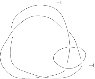
Refer to caption

Figure 8. Kirby calculus description of Y−2Y_{-2}.

This three-manifold can alternately be given as a plumbing as in Figure 9, substituting in k=−2k=-2.

Refer to caption

Figure 9. Plumbing description for YkY_{k}

From the plumbing description, it is clear that Y−2Y_{-2} is obtained from from L⁡(49,40)L(49,40) (which is the manifold obtained by leaving off the vertex labelled by kk) by attaching a single two-handle with framing −2-2. Since w2w_{2} of the plumbing diagram can be represented by the sum of the Poincaré duals of the (−7)(-7)-sphere and the (−5)(-5)-sphere, it follows easily that WW is a spin cobordism. Let 𝔰0\mathfrak{s}_{0} denote the Spinc{\mathrm{Spin}}^{c} structure on WW with c1​(𝔰0)=0c_{1}(\mathfrak{s}_{0})=0. We claim that the map FW,𝔰0∞F^{\infty}_{W,\mathfrak{s}_{0}} is non-trivial. This follows easily from the fact that the map FW,𝔰0+F^{+}_{W,\mathfrak{s}_{0}} is a summand in the map F2F_{2} belonging to a surgery long exact sequence:

...→H​F+​(L⁡(49,40))→H​F+​(Y−2)→H​F+​(L⁡(49,44))→...,\begin{CD}...@>{}>{}>HF^{+}(L(49,40))@>{}>{}>HF^{+}(Y_{-2})@>{}>{}>HF^{+}(L(49,44))@>{}>{}>...,\end{CD}

where L⁡(49,44)L(49,44) is the manifold which is boundary of the plumbing pictured in Figure 9 with k=−1k=-1. Using Proposition 4.8, we see that the correction term for L⁡(49,40)L(49,40) in its spin structure is −2-2, and as usual one can see that the FW,𝔰0∞F^{\infty}_{W,\mathfrak{s}_{0}} decreases degree by 1/21/2. It follows that d−1/2(Y−2)≤−5/2d_{-1/2}(Y_{-2})\leq-5/2. (In fact, it follows from another glance at the above exact sequence that FW,𝔰0+F^{+}_{W,\mathfrak{s}_{0}} can have no kernel, and hence that d−1/2(Y−2)=−5/2d_{-1/2}(Y_{-2})=-5/2.)

Thus, according to Corollary 9.13, it follows that Y−2Y_{-2} is not obtained as the zero-surgery on a one-component knot in S3S^{3} (and, indeed, that Y−2Y_{-2} does not bound any homology S2×D2S^{2}\times D^{2}).

10.3. Alexander polynomials of knots giving lens spaces.

Results from Section 7 (c.f. Corollary 7.5) give, for each pair of relatively prime integers (p,q)(p,q), an explicitly calculable, finite list of symmetric polynomials in TT which contains the Alexander polynomials of all knots K⊂S3K\subset S^{3} with the property that Sp3​(K)≅L⁡(p,q)S^{3}_{p}(K)\cong L(p,q). It is interesting to compare the with the conjecture of Berge [3].

This list is determined as follows. Given (p,q)(p,q), we list the correction terms d⁡(L⁡(p,q),i)d(L(p,q),i) and d⁡(L⁡(p,1),i)d(L(p,1),i) for i=0,…,p−1i=0,...,p-1, as determined in Proposition 4.8. For each multiplicative generator generator h∈(ℤ/p​ℤ)∗h\in(\mathbb{Z}/{p}\mathbb{Z})^{*}, and each c∈ℤ/p​ℤc\in\mathbb{Z}/{p}\mathbb{Z} we define a corresponding sequence tit_{i} (indexed by integers ii) by the formula

0≤2​ti={−d⁡(L⁡(p,q),c+h⋅i)+d⁡(L⁡(p,1),i)if 2​|i|≤p0otherwise.0\leq 2t_{i}=\left\{\begin{array}[]{ll}-d(L(p,q),c+h\cdot i)+d(L(p,1),i)&{\text{if $2|i|\leq p$}}\\ 0&{\text{otherwise.}}\end{array}\right.

If the numbers tit_{i} are all non-negative integers, then there is a Laurent polynomial in TT

Δ⁡(T)=a0+∑i=1∞ai​(Ti+T−i)\Delta(T)=a_{0}+\sum_{i=1}^{\infty}a_{i}(T^{i}+T^{-i})

whose coefficients are given by

ai={ti−1−2​ti+ti+1if i≠01+t−1−2​t0+t1if i=0a_{i}=\left\{\begin{array}[]{ll}t_{i-1}-2t_{i}+t_{i+1}&{\text{if $i\neq 0$}}\\ 1+t_{-1}-2t_{0}+t_{1}&{\text{if $i=0$}}\end{array}\right.

(compare Equation (1)). Let ℱ⁡(p,q){\mathcal{F}}(p,q) denote the set of all symmetric Laruent polynomials obtained in this manner. In particular, observe that the number of polynomials in ℱ⁡(p,q){\mathcal{F}}(p,q) is bounded by pp times the number of integers integers in {1,…,p−1}\{1,...,p-1\} which are relatively prime to pp (note that this is a crude estimate, which can easily be improved, using the conjugation symmetry).

It follows from Corollary 7.5 that if K⊂S3K\subset S^{3} is any knot with the property that Sp3​(K)≅L⁡(p,q)S^{3}_{p}(K)\cong L(p,q), then its Alexander polynomial ΔK\Delta_{K} appears in the list ℱ⁡(p,q){\mathcal{F}}(p,q).

We include here a table of ℱ⁡(p,q){\mathcal{F}}(p,q) for all integers p≤26p\leq 26. To conserve space, we do not display ℱ⁡(p,q){\mathcal{F}}(p,q) when either:

  • •

    q=1q=1 (for then ℱ⁡(p,1)={1}{\mathcal{F}}(p,1)=\{1\}, according to Theorem 1.8),

  • •

    ℱ⁡(p,q)=∅{\mathcal{F}}(p,q)=\emptyset,

  • •

    we have already displayed ℱ⁡(p,q′){\mathcal{F}}(p,q^{\prime}), where qq and q′q^{\prime} are related by q⋅q′≡1(modp)q\cdot q^{\prime}\equiv 1\pmod{p}, because in this case L⁡(p,q′)≅L⁡(p,q)L(p,q^{\prime})\cong L(p,q), so that ℱ⁡(p,q)=ℱ⁡(p,q′){\mathcal{F}}(p,q)={\mathcal{F}}(p,q^{\prime}).

Note that in this list, ℱ⁡(21,16){\mathcal{F}}(21,16) consists of two polynomials (while all other sets displayed consist of a single polynomial).

ℱ⁡(5,4)\displaystyle{\mathcal{F}}(5,4) =\displaystyle= {−1+T−1+T}\displaystyle\{-1+{T^{-1}}+T\}
ℱ⁡(7,4)\displaystyle{\mathcal{F}}(7,4) =\displaystyle= {−1+T−1+T}\displaystyle\{-1+{T^{-1}}+T\}
ℱ⁡(9,7)\displaystyle{\mathcal{F}}(9,7) =\displaystyle= {1+T−2−T−1−T+T2}\displaystyle\{1+T^{-2}-{T^{-1}}-T+T^{2}\}
ℱ⁡(10,9)\displaystyle{\mathcal{F}}(10,9) =\displaystyle= {1+T−6−2​T−5+T−4+T−3−T−2−T2+T3+T4−2​T5+T6}\displaystyle\{1+T^{-6}-{2}\,{T^{-5}}+T^{-4}+T^{-3}-T^{-2}-T^{2}+T^{3}+T^{4}-2\,T^{5}+T^{6}\}
ℱ⁡(11,9)\displaystyle{\mathcal{F}}(11,9) =\displaystyle= {1+T−3−T−2−T2+T3}\displaystyle\{1+T^{-3}-T^{-2}-T^{2}+T^{3}\}
ℱ⁡(11,4)\displaystyle{\mathcal{F}}(11,4) =\displaystyle= {1+T−2−T−1−T+T2}\displaystyle\{1+T^{-2}-{T^{-1}}-T+T^{2}\}
ℱ⁡(13,12)\displaystyle{\mathcal{F}}(13,12) =\displaystyle= {−3+T−6−2​T−5+2​T−4−T−3+2​T−1+2​T−T3+2​T4−2​T5+T6}\displaystyle\{-3+T^{-6}-{2}\,{T^{-5}}+{2}\,{T^{-4}}-T^{-3}+{2}\,{T^{-1}}+2\,T-T^{3}+2\,T^{4}-2\,T^{5}+T^{6}\}
ℱ⁡(13,10)\displaystyle{\mathcal{F}}(13,10) =\displaystyle= {−1+T−3−T−2+T−1+T−T2+T3}\displaystyle\{-1+T^{-3}-T^{-2}+{T^{-1}}+T-T^{2}+T^{3}\}
ℱ⁡(13,9)\displaystyle{\mathcal{F}}(13,9) =\displaystyle= {1+T−3−T−2−T2+T3}\displaystyle\{1+T^{-3}-T^{-2}-T^{2}+T^{3}\}
ℱ⁡(14,11)\displaystyle{\mathcal{F}}(14,11) =\displaystyle= {−1+T−4−T−3+T−1+T−T3+T4}\displaystyle\{-1+T^{-4}-T^{-3}+{T^{-1}}+T-T^{3}+T^{4}\}
ℱ⁡(15,4)\displaystyle{\mathcal{F}}(15,4) =\displaystyle= {−1+T−3−T−2+T−1+T−T2+T3}\displaystyle\{-1+T^{-3}-T^{-2}+{T^{-1}}+T-T^{2}+T^{3}\}
ℱ⁡(16,9)\displaystyle{\mathcal{F}}(16,9) =\displaystyle= {−1+T−4−T−3+T−1+T−T3+T4}\displaystyle\{-1+T^{-4}-T^{-3}+{T^{-1}}+T-T^{3}+T^{4}\}
ℱ⁡(17,16)\displaystyle{\mathcal{F}}(17,16) =\displaystyle= {−3+T−9−2T−8+T−7+T−6−2T−4+T−3+T−2+\displaystyle\{-3+T^{-9}-{2}\,{T^{-8}}+T^{-7}+T^{-6}-{2}\,{T^{-4}}+T^{-3}+T^{-2}+
T−1+T+T2+T3−2T4+T6+T7−2T8+T9}\displaystyle{T^{-1}}+T+T^{2}+T^{3}-2\,T^{4}+T^{6}+T^{7}-2\,T^{8}+T^{9}\}
ℱ⁡(17,15)\displaystyle{\mathcal{F}}(17,15) =\displaystyle= {1+T−7−2​T−6+2​T−5−T−4+T−2−T−1−T+T2−T4+2​T5−2​T6+T7}\displaystyle\{1+T^{-7}-{2}\,{T^{-6}}+{2}\,{T^{-5}}-T^{-4}+T^{-2}-{T^{-1}}-T+T^{2}-T^{4}+2\,T^{5}-2\,T^{6}+T^{7}\}
ℱ⁡(17,13)\displaystyle{\mathcal{F}}(17,13) =\displaystyle= {1+T−4−T−3+T−2−T−1−T+T2−T3+T4}\displaystyle\{1+T^{-4}-T^{-3}+T^{-2}-{T^{-1}}-T+T^{2}-T^{3}+T^{4}\}
ℱ⁡(18,13)\displaystyle{\mathcal{F}}(18,13) =\displaystyle= {1+T−5−T−4+T−2−T−1−T+T2−T4+T5}\displaystyle\{1+T^{-5}-T^{-4}+T^{-2}-{T^{-1}}-T+T^{2}-T^{4}+T^{5}\}
ℱ⁡(19,17)\displaystyle{\mathcal{F}}(19,17) =\displaystyle= {1+T−9−2​T−8+T−7+T−6−T−5+T−3−T−2−T2+T3−T5+T6+T7−2​T8+T9}\displaystyle\{1+T^{-9}-{2}\,{T^{-8}}+T^{-7}+T^{-6}-T^{-5}+T^{-3}-T^{-2}-T^{2}+T^{3}-T^{5}+T^{6}+T^{7}-2\,T^{8}+T^{9}\}
ℱ⁡(19,16)\displaystyle{\mathcal{F}}(19,16) =\displaystyle= {−1+T−6−T−5+T−2+T2−T5+T6}\displaystyle\{-1+T^{-6}-T^{-5}+T^{-2}+T^{2}-T^{5}+T^{6}\}
ℱ⁡(19,11)\displaystyle{\mathcal{F}}(19,11) =\displaystyle= {1+T−5−T−4+T−2−T−1−T+T2−T4+T5}\displaystyle\{1+T^{-5}-T^{-4}+T^{-2}-{T^{-1}}-T+T^{2}-T^{4}+T^{5}\}
ℱ⁡(19,5)\displaystyle{\mathcal{F}}(19,5) =\displaystyle= {1+T−4−T−3+T−2−T−1−T+T2−T3+T4}\displaystyle\{1+T^{-4}-T^{-3}+T^{-2}-{T^{-1}}-T+T^{2}-T^{3}+T^{4}\}
ℱ⁡(20,9)\displaystyle{\mathcal{F}}(20,9) =\displaystyle= {1+T−6−T−5+T−3−T−2−T2+T3−T5+T6}\displaystyle\{1+T^{-6}-T^{-5}+T^{-3}-T^{-2}-T^{2}+T^{3}-T^{5}+T^{6}\}
ℱ⁡(21,16)\displaystyle{\mathcal{F}}(21,16) =\displaystyle= {−1+T−5−T−4+T−3−T−2+T−1+T−T2+T3−T4+T5,\displaystyle\{-1+T^{-5}-T^{-4}+T^{-3}-T^{-2}+{T^{-1}}+T-T^{2}+T^{3}-T^{4}+T^{5},
−1+T−6−T−5+T−2+T2−T5+T6}\displaystyle-1+T^{-6}-T^{-5}+T^{-2}+T^{2}-T^{5}+T^{6}\}
ℱ⁡(22,9)\displaystyle{\mathcal{F}}(22,9) =\displaystyle= {1+T−6−T−5+T−3−T−2−T2+T3−T5+T6}\displaystyle\{1+T^{-6}-T^{-5}+T^{-3}-T^{-2}-T^{2}+T^{3}-T^{5}+T^{6}\}
ℱ⁡(23,18)\displaystyle{\mathcal{F}}(23,18) =\displaystyle= {−1+T−7−T−6+T−4−T−3+T−1+T−T3+T4−T6+T7}\displaystyle\{-1+T^{-7}-T^{-6}+T^{-4}-T^{-3}+{T^{-1}}+T-T^{3}+T^{4}-T^{6}+T^{7}\}
ℱ⁡(23,16)\displaystyle{\mathcal{F}}(23,16) =\displaystyle= {−1+T−7−T−6+T−3−T−2+T−1+T−T2+T3−T6+T7}\displaystyle\{-1+T^{-7}-T^{-6}+T^{-3}-T^{-2}+{T^{-1}}+T-T^{2}+T^{3}-T^{6}+T^{7}\}
ℱ⁡(23,6)\displaystyle{\mathcal{F}}(23,6) =\displaystyle= {−1+T−5−T−4+T−3−T−2+T−1+T−T2+T3−T4+T5}\displaystyle\{-1+T^{-5}-T^{-4}+T^{-3}-T^{-2}+{T^{-1}}+T-T^{2}+T^{3}-T^{4}+T^{5}\}
ℱ⁡(25,24)\displaystyle{\mathcal{F}}(25,24) =\displaystyle= {−5+2T−12−3T−11+2T−9+T−8−4T−7+2T−6+2T−5−2T−4−T−3+2T−2+2T−1\displaystyle\{-5+{2}\,{T^{-{12}}}-{3}{T^{-{11}}}+{2}\,{T^{-9}}+T^{-8}-{4}{T^{-7}}+{2}\,{T^{-6}}+{2}\,{T^{-5}}-{2}\,{T^{-4}}-T^{-3}+{2}\,{T^{-2}}+{2}\,{T^{-1}}
+2T+2T2−T3−2T4+2T5+2T6−4T7+T8+2T9−3T11+2T12}\displaystyle+2\,T+2\,T^{2}-T^{3}-2\,T^{4}+2\,T^{5}+2\,T^{6}-4\,T^{7}+T^{8}+2\,T^{9}-3\,T^{11}+2\,T^{12}\}
ℱ⁡(25,21)\displaystyle{\mathcal{F}}(25,21) =\displaystyle= {1+T−9−2​T−8+2​T−7−T−6+T−4−T−3+T−2−T−1−T+T2−T3+T4−T6+2​T7−2​T8+T9}\displaystyle\{1+T^{-9}-{2}\,{T^{-8}}+{2}\,{T^{-7}}-T^{-6}+T^{-4}-T^{-3}+T^{-2}-{T^{-1}}-T+T^{2}-T^{3}+T^{4}-T^{6}+2\,T^{7}-2\,T^{8}+T^{9}\}
ℱ⁡(25,19)\displaystyle{\mathcal{F}}(25,19) =\displaystyle= {1+T−6−T−5+T−4−T−3+T−2−T−1−T+T2−T3+T4−T5+T6}\displaystyle\{1+T^{-6}-T^{-5}+T^{-4}-T^{-3}+T^{-2}-{T^{-1}}-T+T^{2}-T^{3}+T^{4}-T^{5}+T^{6}\}
ℱ⁡(25,16)\displaystyle{\mathcal{F}}(25,16) =\displaystyle= {1+T−8−T−7+T−4−T−3+T−2−T−1−T+T2−T3+T4−T7+T8}\displaystyle\{1+T^{-8}-T^{-7}+T^{-4}-T^{-3}+T^{-2}-{T^{-1}}-T+T^{2}-T^{3}+T^{4}-T^{7}+T^{8}\}
ℱ⁡(25,14)\displaystyle{\mathcal{F}}(25,14) =\displaystyle= {−1+T−7−T−6+T−4−T−3+T−1+T−T3+T4−T6+T7}\displaystyle\{-1+T^{-7}-T^{-6}+T^{-4}-T^{-3}+{T^{-1}}+T-T^{3}+T^{4}-T^{6}+T^{7}\}
ℱ⁡(26,25)\displaystyle{\mathcal{F}}(26,25) =\displaystyle= {1+3T−14−5T−13+T−12+T−11+T−10+T−9−3T−8+T−6+T−5+T−4−2T−3−T−2+T−1\displaystyle\{1+{3}\,{T^{-14}}-{5}\,{T^{-{13}}}+T^{-12}+T^{-11}+T^{-10}+T^{-9}-{3}\,{T^{-8}}+T^{-6}+T^{-5}+T^{-4}-{2}\,{T^{-3}}-T^{-2}+{T^{-1}}
+T−T2−2T3+T4+T5+T6−3T8+T9+T10+T11+T12−5T13+3T14}\displaystyle+T-T^{2}-2\,T^{3}+T^{4}+T^{5}+T^{6}-3\,T^{8}+T^{9}+T^{10}+T^{11}+T^{12}-5\,T^{13}+3\,T^{14}\}
ℱ⁡(26,23)\displaystyle{\mathcal{F}}(26,23) =\displaystyle= {−1+T−12−2T−11+T−10+T−9−T−8+T−5−T−4+T−2\displaystyle\{-1+T^{-12}-{2}\,{T^{-{11}}}+T^{-10}+T^{-9}-T^{-8}+T^{-5}-T^{-4}+T^{-2}
+T2−T4+T5−T8+T9+T10−2T11+T12}\displaystyle+T^{2}-T^{4}+T^{5}-T^{8}+T^{9}+T^{10}-2\,T^{11}+T^{12}\}

References

  • [1] M. F. Atiyah, V. K. Patodi, and I. M. Singer. Spectral asymmetry and Riemannian geometry. II. Math. Proc. Cambridge Philos. Soc, 78(3):405–432, 1975.
  • [2] D. M. Austin. Equivariant Floer groups for binary polyhedral spaces. Math. Ann., 302(2):295–322, 1995.
  • [3] J. O. Berge. Some knots with surgeries giving lens spaces. Unpublished manuscript.
  • [4] P. Braam and S. K. Donaldson. Floer’s work on instanton homology, knots, and surgery. In H. Hofer, C. H. Taubes, A. Weinstein, and E. Zehnder, editors, The Floer Memorial Volume, number 133 in Progress in Mathematics, pages 195–256. Birkhäuser, 1995.
  • [5] M. Culler, C. McA. Gordon, J. Luecke, and P. B. Shalen. Dehn surgery on knots. Ann. of Math., 125(2):237–300, 1987.
  • [6] S. K. Donaldson. An application of gauge theory to four-dimensional topology. J. Differential Geom., 18(2):279–315, 1983.
  • [7] N. D. Elkies. A characterization of the Zn{Z}^{n} lattice. Math. Res. Lett., 2(3):321–326, 1995.
  • [8] R. Fintushel and R. J. Stern. Constructing lens spaces by surgery on knots. Math. Z., 175(1):33–51, 1980.
  • [9] R. Fintushel and R. J. Stern. Immersed spheres in 44-manifolds and the immersed Thom conjecture. Turkish J. Math, 19(2):145–157, 1995.
  • [10] R. Fintushel and R. J. Stern. Using Floer’s exact triangle to compute Donaldson invariants. In The Floer memorial volume, number 133 in Progr. Math., pages 435–444. Birkhäuser, 1995.
  • [11] A. Floer. Instanton homology, surgery, and knots. In Geometry of Low-Dimensional Manifolds, 1 (Durham, 1989), volume 150 of London Math. Soc. Lecture Note Ser., pages 97–114, 1990.
  • [12] K. A. Frøyshov. The Seiberg-Witten equations and four-manifolds with boundary. Math. Res. Lett, 3:373–390, 1996.
  • [13] C. McA. Gordon. Some aspects of classical knot theory, pages pp. 1–60. Number 685 in Lecture Notes in Math. Springer-Verlag, 1978.
  • [14] C. McA. Gordon. Dehn surgery on knots. In Proceedings of the International Congress of Mathematicians Vol. I (Kyoto, 1990), pages 631–642. Springer-Verlag, 1991.
  • [15] J. Hoste. Sewn-up rr-link exteriors. Pacific J. Math., 112(2):347–382, 1984.
  • [16] P. B. Kronheimer and T. S. Mrowka. The genus of embedded surfaces in the projective plane. Math. Research Letters, 1:797–808, 1994.
  • [17] J. W. Morgan, T. S. Mrowka, and D. Ruberman. The L2L^{2}-Moduli Space and a Vanishing Theorem for Donaldson Polynomial Invariants. Number II in Monographs in Geometry and Topology. International Press, 1994.
  • [18] J. W. Morgan, T. S. Mrówka, and Z. Szabó. Product formulas along T3T^{3} for Seiberg-Witten invariants. Math. Res. Lett., 4(6):915–929, 1997.
  • [19] J. W. Morgan, Z. Szabó, and C. H. Taubes. A product formula for Seiberg-Witten invariants and the generalized Thom conjecture. J. Differential Geometry, 44:706–788, 1996.
  • [20] P. S. Ozsváth and Z. Szabó. Holomorphic disks and three-manifold invariants: properties and applications. math.SG/0105202, 2001.
  • [21] P. S. Ozsváth and Z. Szabó. Holomorphic disks and topological invariants for rational homology three-spheres. math.SG/0101206, 2001.
  • [22] P. S. Ozsváth and Z. Szabó. Holomorphic triangles and invariants for smooth four-manifolds. math.SG/0110169, 2001.
  • [23] P. S. Ozsváth and Z. Szabó. Holomorphic triangle invariants and the topology of symplectic four-manifolds. math.SG/0201059, 2002.
  • [24] P. S. Ozsváth and Z. Szabó. On the Floer homology of plumbed three-manifolds. In preparation, 2002.
  • [25] S. Strle. Bounds on genus and geometric intersections from cylindrical end moduli spaces. math.DG/0202178, 2002.