Iterated Integrals and Algebraic Cycles: Examples and ProspectsThanks: Supported in part by grants from the National Science Foundation.

Richard Hain Address: Department of Mathematics
Duke University
Durham, NC 27708-0320 Email address: hain@math.duke.edu

Date: August 11, 2026

The goal of this paper is to produce evidence for a connection between the work of Kuo-Tsai Chen on iterated integrals and de Rham homotopy theory on the one hand, and the work of Wei-Liang Chow on algebraic cycles on the other. Evidence for such a profound link has been emerging steadily since the early 1980s when Carlson, Clemens and Morgan [13] and Bruno Harris [40] gave examples where the periods of non-abelian iterated integrals coincide with the periods of homologically trivial algebraic cycles. Algebraic cycles and the classical Chow groups are nowadays considered in the broader arena of motives, algebraic $K$ -theory and higher Chow groups. This putative connection is best viewed in this larger context. Examples relating iterated integrals and motives go back to Bloch’s work on the dilogarithm and regulators [9] in the mid 1970s, which was developed further by Beilinson [7] and Deligne (unpublished). Further evidence to support a connection between de Rham homotopy theory and iterated integrals includes [48, 4, 30, 57, 50, 22, 37, 59, 58, 25, 38, 51, 55, 19, 60, 20]. Chen would have been delighted by these developments, as he believed iterated integrals and loopspaces contain non-trivial geometric information and would one day become a useful mathematical tool outside topology.

The paper is largely expository, beginning with an introduction to iterated integrals and Chen’s de Rham theorems for loop spaces and fundamental groups. It does contain some novelties, such as the de Rham theorem for fundamental groups of smooth algebraic curves in terms of “meromorphic iterated integrals of the second kind,” and the treatment of the Hodge and weight filtrations of the algebraic de Rham cohomology of loop spaces of algebraic varieties in characteristic zero. A generalization of the theorem of Carlson-Clemens-Morgan in Section 10 is presented, although the proof is not complete for lack of a rigorous theory of iterated integrals of currents. Even though there is no rigorous theory, iterated integrals of currents are a useful heuristic tool which illuminate the combinatorial and geometric content of iterated integrals. The development of this theory should be extremely useful for applications of de Rham theory to the study of algebraic cycles. The heuristic theory is discussed in Section 6.

A major limitation of iterated integrals and rational homotopy theory of non-simply connected spaces is that they usually only give information about nilpotent completions of topological invariants. This is particularly limiting in many cases, such as when studying knots and moduli spaces of curves. By using iterated integrals of twisted differential forms or certain convergent infinite sums of iterated integrals, one may get beyond nilpotence. Non-nilpotent iterated integrals and their Hodge theory should emerge when studying the periods of extensions of variations of Hodge structure associated to algebraic cycles in complex algebraic manifolds, when one spreads the variety and the cycles. Some developments in the de Rham theory, which originate with a suggestion of Deligne, are surveyed in Section 12.

Iterated integrals are the “de Rham realization” of the cosimplicial version of the cobar construction, a construction which goes back to Adams [2]. The paper ends with an exposition of the cobar construction. Logically, the paper could have begun with it, and some readers may prefer to start there. I hope that the examples in the paper will lead the reader to the conclusion, first suggested by Wojtkowiak [57], that the cosimplicial version of the cobar construction is important in algebraic geometry, and that the numerous occurrences of iterated integrals as periods of cycles and motives are not unrelated, but are the de Rham manifestation of a deeper connection between motives and the cobar construction.

This paper complements the survey article [33], which emphasizes the fundamental group. I highly recommend Chen’s Bulletin article [15]; it surveys most of his work, and contains complete proofs of many of his important theorems; it also contains a useful account of the cobar construction. Polylogarithms are discussed from the point of view of iterated integrals in [34].

There is much beautiful mathematics that connects iterated integrals to motives which is not covered in this paper. Most notable are Drinfeld’s work [23], in particular his associator, which appears in the study of the motivic fundamental group of ${\mathbb{P}}^{1}-\{0,1,\infty\}$ , and the Kontsevich integral [45], which appears in the construction of Vassiliev invariants.

Acknowledgements: It is a great pleasure to acknowledge all those who have inspired and contributed to my understanding of iterated integrals, most notably Kuo-Tsai Chen, my thesis adviser, who introduced me to them; Pierre Cartier, who influenced the way I think about them; and, Dennis Sullivan who influenced me and many others through his seminal paper [54] which still contains many paths yet to be explored.

1. Differential Forms on Path Spaces

Denote the space of piece wise smooth paths $\gamma:[0,1]\to X$ in a smooth manifold $X$ by $PX$ . Chen’s iterated integrals can be defined using any reasonable definition of differential form on $PX$ , such at the one used by Chen (see [15], for example). We shall denote the de Rham complex of $X$ , $PX$ , etc by $E^{\bullet}(X)$ , $E^{\bullet}(PX)$ , etc.

We will say that a function $\alpha:N\to PX$ from a smooth manifold into $PX$ is smooth if the mapping

\phi_{\alpha}:[0,1]\times N\to X

defined by $(t,x)\mapsto\alpha(x)(t)$ is piecewise smooth in the sense that there is a partition $0=t_{0}<t_{1}<\dots<t_{n-1}<t_{n}=1$ of $[0,1]$ such that the restriction of $\phi_{\alpha}$ to each $[t_{j-1},t_{j}]\times N$ is smooth.¹¹ 1 Recall that a function $f:K\to{\mathbb{R}}$ from a subset $K$ of ${\mathbb{R}}^{N}$ is smooth if there exists an open neighbourhood $U$ of $K$ in ${\mathbb{R}}^{N}$ and a smooth function $g:U\to{\mathbb{R}}$ whose restriction to $K$ is $f$ .

They key features of the de Rham complex should satisfy are:

(i)

$E^{\bullet}(PX)$ is a differential graded algebra;
(ii)

if $N$ is a smooth manifold and $\alpha:N\to PX$ is smooth, then there is an induced homomorphism

$\alpha^{\ast}:E^{\bullet}(PX)\to E^{\bullet}(N)$

of differential graded algebras;
(iii)

if $D$ and $Q$ are manifolds and $D\times PX\to Q$ is smooth (that is, $D\times N\to D\times PX\to Q$ is smooth for all smooth $N\to PX$ , where $N$ is a manifold), then there is an induced dga homomorphism

$E^{\bullet}(Q)\to E^{\bullet}(D\times PX).$
(iv)

If $D$ is compact oriented (possibly with boundary) of dimension $n$ and $p:D\times PX\to PX$ is the projection, then one has the integration over the fiber mapping

$p_{\ast}:E^{k+n}(D\times PX)\to E^{k}(PX)$

which satisfies

$p_{\ast}d\pm d\,p_{\ast}=(p|_{\partial D})_{\ast}$

Chen’s approach is particularly elementary and direct. For him, a smooth $k$ -form on $PX$ is a collection $w=(w_{\alpha})$ of smooth $k$ -forms, indexed by the smooth mappings $\alpha:N_{\alpha}\to PX$ , where $w_{\alpha}\in E^{k}(N_{\alpha})$ . These are required to satisfy the following compatibility condition: if $f:N_{\alpha}\to N_{\beta}$ is smooth, then

w_{\alpha}=f^{\ast}w_{\beta}.

Exterior derivatives are defined by setting $d(w_{\alpha})=(dw_{\alpha})$ . Exterior products are defined similarly. The de Rham complex of $PX$ is a differential graded algebra.

This definition generalizes easily to other natural subspaces $W$ of $PX$ , such as loop spaces and fixed end point path spaces. Just replace $PX$ by $W$ and consider only those $\alpha:N_{\alpha}\to PX$ that factor through the inclusion $W\hookrightarrow PX$ . It also generalizes to products of such $W$ with a smooth manifold $Q$ . To define a smooth form $w$ on $Q\times W$ , one need specify only the $w_{\alpha}$ for those smooth mappings $\alpha$ of the form $\operatorname{id}\times\alpha:Q\times N\to Q\times W$ .

Lest this seem ad hoc, I should mention that Chen developed an elementary and efficient theory of “differentiable spaces”, the category of which contains the category of smooth manifolds and smooth maps, which is closed under taking path spaces and subspaces. Each differentiable space has a natural de Rham complex which is functorial under smooth maps. The details can be found in his Bulletin article [15].

2. Iterated Integrals

This is a brief sketch of iterated integrals. I have been deliberately vague about the signs as they depend on choices of conventions which do not play a crucial role in the theory. Another reason I have omitted them in this discussion is that, by using different sign conventions from those of Chen, I believe one should be able to make the signs in many formulas conform more to standard homological conventions. Chen’s sign conventions are given in Theorem 7.2 and will be used in all computations in this paper.

Suppose that $w_{1},\dots,w_{r}$ are differential forms on $X$ , all of positive degree. The iterated integral

\int w_{1}w_{2}\dots w_{r}

is a differential form on $PX$ of degree $-r+\deg w_{1}+\deg w_{2}+\cdots+\deg w_{r}$ . Up to a sign (which depends on one’s conventions)

\int w_{1}w_{2}\dots w_{r}=\pi_{\ast}\phi^{\ast}(p_{1}^{\ast}w_{1}\wedge p_{2}^{\ast}w_{2}\wedge\cdots\wedge p_{r}^{\ast}w_{r})

where

(i)

$p_{j}:X^{r}\to X$ is projection onto the $j$ th factor,
(ii)

$\Delta^{r}=\{(t_{1},\dots,t_{r}):0\leq t_{1}\leq t_{2}\leq\cdots\leq t_{r}\leq 1\}$ is the time ordered form of the standard $r$ -simplex,
(iii)

$\phi:\Delta^{r}\times PX\to X^{r}$ is the sampling map

$\phi(t_{1},\dots,t_{r},\gamma)=(\gamma(t_{1}),\gamma(t_{2}),\dots,\gamma(t_{r})),$
(iv)

$\pi_{\ast}$ denotes integration over the fiber of the projection

$\pi:\Delta^{r}\times PX\to PX.$

When each $w_{j}$ is a 1-form, $\int w_{1}\dots w_{r}$ is a function $PX\to{\mathbb{R}}$ . Its value on the path $\gamma:[0,1]\to X$ is the time ordered integral

(1)

\int_{\gamma}w_{1}\dots w_{r}:=\int_{0\leq t_{1}\leq t_{2}\leq\cdots\leq t_{n}\leq 1}f_{1}(t_{1})\dots f_{r}(t_{r})dt_{1}\dots dt_{r},

where $\gamma^{\ast}w_{j}=f_{j}(t)dt$ . Iterated integrals of degree zero are called iterated line integrals.

The space of iterated integrals on $PX$ is the subspace $\mathit{Ch}^{\bullet}(PX)$ of its de Rham complex spanned by all differential forms of the form

(2)

p_{0}^{\ast}w^{\prime}\wedge p_{1}^{\ast}w^{\prime\prime}\wedge\int w_{1}\dots w_{r}

where for $a\in[0,1]$ , $p_{a}:PX\to X$ is the evaluation at time $a$ mapping $\gamma\mapsto\gamma(a)$ .

If $W$ is a subspace of $PX$ (such as a fixed end point path space, the free loop space, a pointed loop space), we shall denote the subspace of its de Rham complex generated by the restrictions of iterated integrals to it by $\mathit{Ch}^{\bullet}(W)$ and call it the Chen complex of $W$ . It is naturally filtered by length:

\mathit{Ch}_{0}^{\bullet}(W)\subseteq\mathit{Ch}_{1}^{\bullet}(W)\subseteq\mathit{Ch}_{2}^{\bullet}(W)\subseteq\cdots\subseteq\mathit{Ch}^{\bullet}(W),

where $\mathit{Ch}_{s}^{\bullet}(W)$ consists of all iterated integrals that are sums of terms (2) where $r\leq s$ .

The standard formula

\pi_{\ast}d\pm d\,\pi_{\ast}=(\pi|_{\partial\Delta^{r}})_{\ast}

implies that iterated integrals are closed under exterior differentiation and that, with suitable signs (depending on one’s conventions),

d\int w_{1}\dots w_{r}=\sum_{j=1}^{r}\pm\int w_{1}\dots dw_{j}\dots w_{r}\cr+\sum_{j=1}^{r-1}\pm\int w_{1}\dots w_{j-1}(w_{j}\wedge w_{j+1})w_{j+2}\dots w_{r}\cr\pm\bigg(\int w_{1}\dots w_{r-1}\bigg)\wedge p_{1}^{\ast}w_{r}\pm p_{0}^{\ast}w_{1}\wedge\int w_{2}\dots w_{r}.

This implies that each $\mathit{Ch}_{s}^{\bullet}(PX)$ , and thus each $\mathit{Ch}_{s}^{\bullet}(W)$ , is closed under exterior differentiation.

The standard triangulation²² 2 This is $\Delta^{r}\times\Delta^{s}=\bigcup_{\sigma\in{\mathrm{s}h}(r,s)}\{(t_{\sigma(1)},t_{\sigma(2)},\dots,t_{\sigma(r+s)}):0\leq t_{1}\leq\dots\leq t_{r}\leq 1,0\leq t_{r+1}\leq\dots\leq t_{r+s}\leq 1\}$ of $\Delta^{r}\times\Delta^{s}$ gives the shuffle product formula

(3)

\int w_{1}\dots w_{r}\wedge\int w_{r+1}\dots w_{r+s}=\sum_{\sigma\in{\mathrm{s}h}(r,s)}\pm\int w_{\sigma(1)}w_{\sigma(2)}\dots w_{\sigma(r+s)}

where ${\mathrm{s}h}(r,s)$ denotes the set of shuffles of type $(r,s)$ — that is, those permutations $\sigma$ of $\{1,2,\dots,r+s\}$ such that

\sigma^{-1}(1)<\sigma^{-1}(2)<\cdots<\sigma^{-1}(r)\text{ and }\cr\sigma^{-1}(s+1)<\sigma^{-1}(s+2)<\cdots<\sigma^{-1}(s+r).

With this product, $\mathit{Ch}^{\bullet}(W)$ is a differential graded algebra (dga).

In many applications, one considers the restrictions of iterated integrals to the fixed end-point path spaces

P_{x,y}X:=\{\gamma\in PX:\gamma(0)=x,\gamma(1)=y\}.

Multiplication of paths

\mu:P_{x,y}X\times P_{y,z}X\to P_{x,z}X

induces a map of the complex of iterated integrals:³³ 3 Here we use the convention that when $s=0$ , $\int\phi_{1}\dots\phi_{s}=1$ .

\mu^{\ast}\int w_{1}\dots w_{r}=\sum_{j=1}^{r}\pi_{1}^{\ast}\int w_{1}\dots w_{j}\wedge\pi_{2}^{\ast}\int w_{j+1}\dots w_{r}

where $\pi_{1}$ and $\pi_{2}$ denote the projections onto the first and second factors of $P_{x,y}X\times P_{y,z}X$ . The inverse mapping

P_{x,y}X\to P_{y,x}X,\qquad\gamma\mapsto\gamma^{-1}

induces the “antipode”

\int w_{1}\dots w_{r}\mapsto\pm\int w_{r}\dots w_{1}.

The closed iterated line integrals $H^{0}(\mathit{Ch}^{\bullet}(P_{x,y}X))$ are precisely those iterated line integrals that are constant on homotopy classes of paths relative to their endpoints.

When $x=y$ , the Chen complex of $P_{x,x}X$ is a differential graded Hopf algebra with diagonal

\int w_{1}\dots w_{r}\mapsto\sum_{j=1}^{r}\int w_{1}\dots w_{j}\otimes\int w_{j+1}\dots w_{r}.

Its cohomology $H^{\bullet}(Ch^{\bullet}(P_{x,x}X))$ is a graded Hopf algebra with antipode. Each element of $H^{\bullet}(Ch^{\bullet}(P_{x,x}X))$ defines a function $\pi_{1}(X,x)\to{\mathbb{R}}$ .

Restricting elements of $\mathit{Ch}^{\bullet}(P_{x,x}X)$ to the constant loop $c_{x}$ at $x$ defines a natural augmentation

Ch^{\bullet}(P_{x,x}X)\to{\mathbb{R}}.

Denote its kernel by $I\mathit{Ch}^{\bullet}(P_{x,x}X)$ . These are the iterated integrals on the loop space $P_{x,x}X$ “with trivial constant term.”

Of course, if one takes iterated integrals of complex-valued forms $E^{\bullet}(X)_{\mathbb{C}}$ , then one obtains complex-valued iterated integrals. We shall denote the Chen complex of complex-valued iterated integrals by $\mathit{Ch}^{\bullet}(PX)_{\mathbb{C}}$ , $\mathit{Ch}^{\bullet}(P_{x,y}X)_{\mathbb{C}}$ , etc.

3. Loop Space de Rham Theorems

Chen proved many useful de Rham type theorems. (A comprehensive list can be found in Section 2 of [30].) In this section we present those of most immediate interest.

Theorem 3.1.

If $X$ is a simply connected manifold, then integration induces a natural Hopf algebra isomorphism

H^{\bullet}(\mathit{Ch}^{\bullet}(P_{x,x}X))\cong H^{\bullet}(P_{x,x}X;{\mathbb{R}}).

This, combined with standard algebraic topology, gives a de Rham theorem for homotopy groups of simply connected manifolds. First a review of the topology:

Suppose that $(Z,x)$ is a connected, pointed topological space and that $A$ is any coefficient ring. Consider the adjoint

h^{t}:H^{\bullet}(Z;A)\to\operatorname{Hom}_{\mathbb{Z}}(\pi_{\bullet}(Z,z),A)

of the Hurewicz homomorphism. An element of $H^{\bullet}(Z;A)$ is decomposable if it is in the image of the cup product mapping

H^{>0}(Z;A)\otimes H^{>0}(Z;A)\to H^{\bullet}(Z;A).

The set of indecomposable elements of the ring $H^{\bullet}(Z;A)$ is defined by

QH^{\bullet}(Z;A):=H^{\bullet}(Z;A)/\text{\lx@text@lbrace the decomposable elements\lx@text@rbrace}.

Since the cohomology ring of a sphere has no decomposables, the kernel of $h^{t}$ contains the decomposable elements of $H^{\bullet}(Z;A)$ , and therefore induces a mapping

e:QH^{\bullet}(Z;A)\to\operatorname{Hom}_{\mathbb{Z}}(\pi_{\bullet}(Z,z),A).

Typically, this mapping is far from being an isomorphism. However, if $A$ is a field of characteristic zero and $Z$ is a connected $H$ -space, then $e$ is an isomorphism. (This is a Theorem of Cartan and Serre — cf. [47].)

When $X$ is simply connected, $P_{x,x}X$ is a connected $H$ -space. Chen’s de Rham theorem and the Cartan-Serre Theorem imply that integration induces an isomorphism

QH^{j}(P_{x,x}X;{\mathbb{R}})\stackrel{{\scriptstyle\simeq}}{{\longrightarrow}}\operatorname{Hom}(\pi_{j}(P_{x,x},c_{x}),{\mathbb{R}})\cong\operatorname{Hom}(\pi_{j+1}(X,x),{\mathbb{R}})

for each $j$ .

There is a canonical subcomplex $Q\mathit{Ch}^{\bullet}(P_{x,x}X)$ of the Chen complex of $P_{x,x}X$ , which is isomorphic to the indecomposable iterated integrals (see [29]) and whose cohomology is $QH^{\bullet}(\mathit{Ch}^{\bullet}(P_{x,x}X))$ . This and Chen’s de Rham Theorem above then yield the following de Rham Theorem for homotopy groups of simply connected spaces:

Theorem 3.2.

Integration induces an isomorphism

H^{\bullet}(Q\mathit{Ch}^{\bullet}(P_{x,x}X))\stackrel{{\scriptstyle\sim}}{{\longrightarrow}}\operatorname{Hom}(\pi_{\bullet}(X,x),{\mathbb{R}})

of degree $+1$ of graded vector spaces.

Both sides of the display in this theorem are naturally “Lie coalgebras.” It is not difficult to show that the integration isomorphism respects this structure.

We now turn our attention to non-simply connected spaces. The augmentation $\epsilon:{\mathbb{Z}}\pi_{1}(X,x)\to{\mathbb{Z}}$ of the integral group ring of $\pi_{1}(X,x)$ is defined by taking each element of the fundamental group to 1. The augmentation ideal $J$ is the kernel of the augmentation $\epsilon$ . The diagonal mapping $\pi_{1}(X,x)\to\pi_{1}(X,x)\times\pi_{1}(X,x)$ induces a coproduct

\Delta:{\mathbb{Z}}\pi_{1}(X,x)\to{\mathbb{Z}}\pi_{1}(X,x)\otimes{\mathbb{Z}}\pi_{1}(X,x).

The most direct statement of Chen’s de Rham theorem for the fundamental group is:

Theorem 3.3 (Chen [14]).

The integration pairing

H^{0}(\mathit{Ch}^{\bullet}(P_{x,x}X))\otimes{\mathbb{Z}}\pi_{1}(X,x)\to{\mathbb{C}}

is a pairing of Hopf algebras under which $H^{0}(\mathit{Ch}_{s}^{\bullet}(P_{x,x}X))$ annihilates $J^{s+1}$ . The induced mapping

H^{0}(\mathit{Ch}_{s}^{\bullet}(P_{x,x}X))\to\operatorname{Hom}_{\mathbb{Z}}({\mathbb{Z}}\pi_{1}(X,x)/J^{s+1},{\mathbb{C}})

is an isomorphism.

An elementary proof is given in [33]. An equivalent statement, more amenable to generalization, will be given in Section 12. A second version uses the $J$ -adic completion

{\mathbb{R}}\pi_{1}(X,x)~\widehat{\!}{\;}:=\lim_{\stackrel{{\scriptstyle\longleftarrow}}{{s}}}{\mathbb{R}}\pi_{1}(X,x)/J^{s}

of ${\mathbb{R}}\pi_{1}(X,x)$ . It is a complete Hopf algebra (cf. [52, Appendix A]), with diagonal

\Delta:{\mathbb{R}}\pi_{1}(X,x)~\widehat{\!}{\;}\to{\mathbb{R}}\pi_{1}(X,x)~\widehat{\!}{\;}\,\hat{\otimes}{\mathbb{R}}\pi_{1}(X,x)~\widehat{\!}{\;}

induced by that of ${\mathbb{R}}\pi_{1}(X,x)$ .

Corollary 3.4.

If $H^{1}(X;{\mathbb{R}})$ is finite dimensional, then integration induces a natural homomorphism

{\mathbb{R}}\pi_{1}(X,x)~\widehat{\!}{\;}\to\operatorname{Hom}(H^{0}(\mathit{Ch}_{s}^{\bullet}(P_{x,x}X)),{\mathbb{R}})

of complete Hopf algebras.

Of course, each of these theorems holds with complex coefficients if we begin with complex-valued forms.

Remark 3.5.

It is tempting to think that one can extend Chen’s loop space de Rham theorem, or its homotopy version, to a de Rham theorem for higher homotopy groups of non-simply connected spaces. While this is true for “nilpotent spaces” (which include Lie groups), it is most definitely not true for most non-simply connected spaces that one meets in day-to-day life. In fact, Example 7.5 shows that there is unlikely to be any reasonable statement. One point we wish to make in this paper, however, is that in arithmetic and algebraic geometry, the cohomology of iterated integrals is intrinsic and may be a more interesting and geometric invariant of a complex algebraic variety than its higher homotopy groups or loop space cohomology.

4. Multi-valued Functions

In this section, we give several examples of interesting multi-valued functions that can be obtained by integrating closed iterated line integrals. Although elementary, these examples are reflections of the relationship between iterated integrals and periods of certain canonical variations of mixed Hodge structure.

The following result is easily proved by pulling back to the universal covering of $X$ and using the definition (1) of iterated line integrals.

Proposition 4.1.

All closed iterated line integrals of length $\leq 2$ on $P_{x,y}X$ are of the form

\sum_{j,k}a_{jk}\int\phi_{j}\phi_{k}+\int\xi+\text{ a constant}

where each $\phi_{j}$ is a closed $1$ -form on $X$ , the $a_{jk}$ are scalars, and $\xi$ is a $1$ -form on $X$ satisfying

d\xi+\sum_{j,k}a_{jk}\,\phi_{j}\wedge\phi_{k}=0.

A relatively closed iterated integral is an element of $\mathit{Ch}^{\bullet}(PX)$ that is closed on $P_{x,y}X$ for all $x,y\in X$ . The iterated line integrals given by the previous result are relatively closed.

Multi-valued functions can be constructed by integrating relatively closed iterated integrals. For example, suppose that $X$ is a Riemann surface and that $w_{1}$ and $w_{2}$ are holomorphic differentials on $X$ . Then

\int w_{1}w_{2}

is closed on each $P_{x,y}X$ . This means that for any fixed point $x_{o}\in X$ , the function

x\mapsto\int_{x_{o}}^{x}w_{1}w_{2}

is a multi-valued function on $X$ . It is easily seen to be holomorphic.

Example 4.2.

If $X={\mathbb{P}}^{1}({\mathbb{C}})-\{0,1,\infty\}$ , then

\int_{0}^{x}\frac{dz}{1-z}\frac{dz}{z}

is a multi-valued holomorphic function on $X$ . In fact, it is Euler’s dilogarithm, whose principal branch in the unit disk is defined by

\operatorname{ln}_{2}(x)=\sum_{n\geq 1}\frac{x^{n}}{n^{2}}.

More generally, the $k$ -logarithm

\operatorname{ln}_{k}(x):=\sum_{n\geq 1}\frac{x^{n}}{n^{k}}\qquad|x|<1

can be expressed as the length $k$ iterated integral

\int_{0}^{x}\frac{dz}{1-z}\overbrace{\frac{dz}{z}\cdots\frac{dz}{z}}^{k-1}

From this integral expression, it is clear that $\ln_{k}$ can be analytically continued to a multi-valued function on ${\mathbb{C}}-\{0,1\}$ .

Note that $\zeta(k)$ , the value of the Riemann zeta function at an integer $k>1$ , is $\ln_{k}(1)$ . More information about iterated integrals and polylogarithms can be found in [34].

More generally, the multiple polylogarithms

L_{m_{1},\dots,m_{n}}(x_{1},\dots,x_{n}):=\sum_{0<k_{1}<\cdots<k_{n}}\frac{x_{1}^{k_{1}}x_{2}^{k_{2}}\dots x_{n}^{k_{n}}}{k_{1}^{m_{1}}k_{2}^{m_{2}}\dots k_{n}^{m_{n}}}\qquad|x_{j}|<1

and their special values, Zagier’s multiple zeta values $\zeta(n_{1},\dots,n_{m})$ , can be expressed as iterated integrals. For example,

L_{1,1}(x,y)=\int_{(0,0)}^{(x,y)}\bigg(\frac{dy}{1-y}\frac{dx}{1-x}+\frac{d(xy)}{1-xy}\bigg(\frac{dy}{1-y}-\frac{dx}{1-x}-\frac{dx}{x}\bigg)\bigg).

This expression defines a well defined multi-valued function on

{\mathbb{C}}^{2}-\{(x,y):xy(1-x)(1-y)(1-xy)\neq 0\}

as the relation

\frac{dy}{1-y}\wedge\frac{dx}{1-x}+\frac{d(xy)}{1-xy}\wedge\bigg(\frac{dy}{1-y}-\frac{dx}{1-x}-\frac{dx}{x}\bigg)=0

holds in the rational 2-forms on ${\mathbb{C}}^{2}$ . Formulas for all multiple polylogarithms and other properties can be found in Zhao’s paper [60].

Closed iterated integrals that involve antiholomorphic 1-forms can also yield multi-valued holomorphic functions.

Proposition 4.3.

Suppose that $X$ is a complex manifold and $w_{1},\dots,w_{n}$ are holomorphic 1-forms. If $\xi$ is a $(1,0)$ form such that

\overline{\partial}\xi+\sum_{j,k}a_{jk}\overline{w}_{j}\wedge w_{k}=0,

then the multi-valued function

F:x\mapsto\sum_{j,k}a_{jk}\int_{x_{o}}^{x}\overline{w}_{j}w_{k}+\int_{x_{o}}^{x}\xi

is well defined and holomorphic.

Proof.

Since each $w_{j}$ is holomorphic,

dF(x)=\sum_{j,k}a_{jk}\bigg(\int_{x_{o}}^{x}\overline{w}_{j}\bigg)w_{k}+\xi.

Since $\xi$ has type $(1,0)$ , $dF$ also has type $(1,0)$ , which implies that $F$ is holomorphic. ∎

Example 4.4.

Take $X$ to be a punctured elliptic curve $E={\mathbb{C}}/\Lambda-\{0\}$ . The point of this example is to show that the logarithm of the associated theta function $\theta(z)$ is a twice iterated integral. We may assume that $\Lambda={\mathbb{Z}}+{\mathbb{Z}}\tau$ where $\tau$ has positive imaginary part. Denote the homology classes of the images of the intervals $[0,1]$ and $[0,\tau]$ by $\alpha$ and $\beta$ , respectively. These form a symplectic basis of $H_{1}(E,{\mathbb{Z}})$ . The normalized abelian differential is $dz$ and $dz=\alpha^{\ast}+\tau\beta^{\ast}$ from which it follows that

d\overline{z}\wedge dz=2i\operatorname{Im}\tau\in H^{2}(E,{\mathbb{C}})\cong{\mathbb{C}}.

The multi-valued differential $\mu=(z-\overline{z})dz$ satisfies

\mu(z+1)=\mu(z)\text{ and }\mu(z+\tau)=\mu(z)+2i\operatorname{Im}\tau dz.

On the other hand, the corresponding theta function $\theta(z):=\theta(z,\tau)$ satisfies

\theta(z+1)=\theta(z)\text{ and }\theta(z+\tau)=\exp(-i\pi\tau-2\pi iz)\theta(z).

Thus

\frac{d\theta}{\theta}(z+1)=\frac{d\theta}{\theta}(z)\text{ and }\frac{d\theta}{\theta}(z+\tau)=\frac{d\theta}{\theta}(z)-2\pi idz.

It follows that

\xi:=\frac{\operatorname{Im}\tau}{\pi}\frac{d\theta}{\theta}+\mu(z)

is a single-valued differential on $E-\{0\}$ of type $(1,0)$ having a logarithmic singularity at 0 which satisfies

d\overline{z}\wedge dz+d\xi=0\text{ in }E^{2}(E-\{0\}).

(In fact, these properties characterize it up to a multiple of $dz$ .) It follows that $\int d\overline{z}dz+\xi$ is relatively closed, so that

x\mapsto\int_{x_{o}}^{x}d\overline{z}\,dz+\xi

is a multi-valued holomorphic function on $E-\{0\}$ . Applying the definition of iterated integrals yields

\log\theta(x)=\log\theta(x_{o})+\frac{\pi}{\operatorname{Im}\tau}\bigg(\int_{x_{o}}^{x}(d\overline{z}\,dz+\xi)-\frac{1}{2}\big(z(x)-\overline{z}(x_{o})\big)^{2}+\frac{1}{2}\big(z(x_{o})-\overline{z}(x_{o})\big)^{2}\bigg),

where $z(x)=\int_{0}^{x}dz$ .⁴⁴ 4 In the language of Beilinson and Levin [8], $\int dz$ is the elliptic logarithm for $E$ , and $\log\theta$ is the elliptic dilogarithm. This example generalizes easily to theta functions of several variables by replacing $E$ by a principally polarized abelian variety $A$ and $E-\{0\}$ by $A-\Theta$ , where $\Theta$ is its theta divisor.

Remark 4.5.

This example can be developed further along the lines of Beilinson [7] and Deligne’s approach to the dilogarithm. (An exposition of this, from the point of view of iterated integrals, can be found in [34].) Set

G=\begin{pmatrix}1&{\mathbb{C}}&{\mathbb{C}}\cr 0&1&{\mathbb{C}}\cr 0&0&1\end{pmatrix}\text{ and }F^{0}G=\begin{pmatrix}1&{\mathbb{C}}&0\cr 0&1&0\cr 0&0&1\end{pmatrix}.

The Lie algebra $\mathfrak{g}$ of $G$ is the Lie algebra of nilpotent upper triangular matrices. Let

w=\begin{pmatrix}0&d\overline{z}&\xi\cr 0&0&dz\cr 0&0&0\end{pmatrix}\in E^{1}(E-\{0\})\otimes\mathfrak{g}.

This form is integrable: $dw+w\wedge w=0$ . It follows that the iterated integral

T=\begin{pmatrix}1&\int d\overline{z}&\int d\overline{z}\,dz+\int\xi\cr 0&1&\int dz\cr 0&0&1\end{pmatrix}

is relatively closed. (See [15] or [33].) It therefore defines a homomorphism

\theta:\pi_{1}(E-\{0\},x_{o})\to G,\quad\gamma\mapsto\langle T,\gamma\rangle

which is the monodromy representation of the flat connection on $(E-\{0\})\times G$ defined by $w$ . There is thus a generalized Abel-Jacobi mapping

\nu:E-\{0\}\to\Gamma\backslash G/F^{0}G

that takes $x$ to $\langle T,\gamma\rangle$ , where $\gamma$ is any path in $E-\{0\}$ from $x_{o}$ to $x$ . It is holomorphic as can be seen directly using the formulas above.

Denote the center

\begin{pmatrix}1&0&{\mathbb{C}}\cr 0&1&0\cr 0&0&1\end{pmatrix}

of $G$ by $Z$ . The quotient $\Gamma\backslash G/(F^{0}G\cdot Z)$ is naturally isomorphic to $E$ itself and the corresponding projection

\Gamma\backslash G/F^{0}G\to E

is a holomorphic ${\mathbb{C}}^{\ast}$ -bundle. The formulas in the previous example show that the section $\nu$ above is a non-zero multiple of the section $\theta$ of the line bundle $L\to E$ associated to the divisor $0\in E$ :

This has an interpretation in terms of variations of MHS, which can be extracted from [39]. The construction given here of the second albanese mapping is special case of the direct construction given in [32]. There is an analogous construction with a similar interpretation where the pair $(E,0)$ is replaced by an abelian variety and its theta divisor $(A,\Theta)$ .

5. Harmonic Volume

Bruno Harris [40] was the first to explicitly combine Hodge theory and and (non-abelian) iterated integrals to obtain periods of algebraic cycles. Suppose that $C$ is a compact Riemann surface of genus 3 or more. Choose any base point $x_{o}\in C$ . Suppose that $L_{1}$ , $L_{2}$ , $L_{3}$ are three disjoint, non-separating simple closed curves on $C$ . Let $\phi_{j}$ be the harmonic representative of the Poincaré dual of $L_{j}$ , $j=1,2,3$ . Since the curves are pairwise disjoint, the product of any two of the $\phi_{j}$ s vanishes in cohomology. Thus there are 1-forms $\phi_{jk}$ such that

d\phi_{jk}+\phi_{j}\wedge\phi_{k}=0

and $\phi_{jk}$ is orthogonal to the $d$ -closed forms. These two conditions characterize the $\phi_{jk}$ . By Proposition 4.1, the iterated line integral

\int\phi_{j}\phi_{k}+\phi_{jk}

is closed in $\mathit{Ch}^{\bullet}(P_{x_{o},x_{o}}C)$ .

Choose loops $\gamma_{j}$ ( $j=1,2,3)$ , based at $x_{o}$ and that are freely homotopic to the $L_{j}$ . Harris sets

I(L_{1},L_{2},L_{3})=\int_{\gamma_{3}}\phi_{1}\phi_{2}+\phi_{12}.

He shows that this integral is independent of the choice of the base point $x_{o}$ and that

I(L_{\sigma(1)},L_{\sigma(2)},L_{\sigma(3)})=\operatorname{sgn}(\sigma)I(L_{1},L_{2},L_{3})

for all permutations $\sigma$ of $\{1,2,3\}$ .

One can also use the $\phi_{j}$ to imbed $C$ into the three torus $T={\mathbb{R}}^{3}/{\mathbb{Z}}^{3}$ . Define $\Phi:C\to T$ by

\Phi(x)=\int_{x_{o}}^{x}(\phi_{1},\phi_{2},\phi_{3})\mod{\mathbb{Z}}^{3}.

If the coordinates in ${\mathbb{R}}^{3}$ are $(z_{1},z_{2},z_{3})$ , then $\Phi^{\ast}dz_{j}=\phi_{j}$ for $j=1,2,3$ . Since $H^{2}(T,{\mathbb{Z}})$ is spanned by the $dz_{j}\wedge dz_{k}$ and since

\int_{\Phi}dz_{j}\wedge dz_{k}=\int_{C}\phi_{j}\wedge\phi_{k}=0,

the image of $C$ is homologous to zero in $T$ . One can therefore find a 3-chain $\Gamma$ in $T$ such that ${\partial}\Gamma=\Phi_{\ast}C$ . Since $\Gamma$ is only well defined up to a 3-cycle, the volume of $\Gamma$ is only well defined mod ${\mathbb{Z}}$ . Harris’s first main result is:

Theorem 5.1.

The volume of $\Gamma$ is congruent to $I(L_{1},L_{2},L_{3})$ mod ${\mathbb{Z}}$ .

By an elementary computation, the span in $\Lambda^{3}H_{1}(C,{\mathbb{Z}})$ of classes $L_{1}\wedge L_{2}\wedge L_{3}$ is the kernel $K$ of the mapping

\Lambda^{3}H_{1}(C,{\mathbb{Z}})\to H_{1}(C,{\mathbb{Z}})

defined by

a\wedge b\wedge c\mapsto(a\cdot b)c+(b\cdot c)a+(c\cdot a)b.

The harmonic volume $I$ thus determines a point in the compact torus $\operatorname{Hom}(K,{\mathbb{R}}/{\mathbb{Z}})$ .

There is a lot more to this story — it has a deep relationship to the algebraic cycle $C_{x}-C_{x}^{-}$ in the jacobian of $C$ . This is best explained in terms of the Hodge theory of the operator $\overline{\partial}$ rather than $d$ . This shall be sketched in Section 9.

6. Iterated Integrals of Currents

There is no rigorous theory of iterated integrals of currents, although such a theory would be useful provided it is not too technical. The theory of iterated integrals makes essential use of the algebra structure of the de Rham complex. The problem one encounters when trying to develop a theory of iterated integrals of currents is that products of currents are only defined when the currents being multiplied (intersected) are sufficiently smooth (or sufficiently transverse). Nonetheless, this point of view is useful, even it if is not rigorous. The paper [28] was an attempt at making these ideas rigorous and using them to study links.

Example 6.1.

In this example $X$ is the unit interval. Suppose that $a_{1},a_{2},\dots,a_{r}$ are distinct points in the interior of the unit interval. Set $w_{j}=\delta(t-a_{j})dt$ , where $\delta(t)$ denotes the Dirac delta function supported at $t=0$ . Let $\gamma:[0,1]\to X=[0,1]$ be the identity path. Recall that $\Delta^{r}$ is the time ordered simplex

\Delta^{r}=\{(t_{1},t_{2},\dots,t_{r}):0\leq t_{1}\leq\dots\leq t_{r}\leq 1\}.

By definition,

	$\displaystyle\int_{\gamma}w_{1}w_{2}\dots w_{r}$	$\displaystyle=\int_{\Delta^{r}}\delta(t_{1}-a_{1})\delta(t_{2}-a_{2})\dots\delta(t_{r}-a_{r})\,dt_{1}dt_{2}\dots dt_{r}$
		$\displaystyle=\int_{\Delta^{r}}\delta_{(a_{1},\dots,a_{r})}(t_{1},\dots,t_{r})\,dt_{1}dt_{2}\dots dt_{r}.$

Since the $a_{j}$ are distinct numbers satisfying $0<a_{j}<1$ ,

\int_{\gamma}w_{1}w_{2}\dots w_{r}=\begin{cases}1&\text{if }a_{1}<a_{2}<\cdots<a_{r},\cr 0&\text{otherwise.}\end{cases}

Example 6.2.

More generally, suppose that $H_{1},\dots,H_{r}$ are real hypersurfaces in a manifold $X$ , each with oriented (and thus trivial) normal bundle. Suppose that $\gamma\in PX$ is transverse to the union of the $H_{j}$ — that is, the endpoints of $\gamma$ do not lie in the union of the $H_{j}$ and $\gamma$ does not pass through any singularity of their union. We can regard each $H_{j}$ as a current, which we shall denote by $w_{j}$ . For such a path $\gamma$ which is transverse to $H_{j}$ ,

\int_{\gamma}w_{j}=(H_{j}\cdot\gamma):=\text{ the intersection number of $H_{j}$ with $\gamma$.}

For simplicity, suppose that $\gamma$ passes through each $H_{j}$ at most once, at time $t=a_{j}$ , say. Then

\gamma^{\ast}w_{j}=\epsilon_{j}\delta_{j}(t-a_{j})

where $\epsilon_{j}$ is 1 if $\gamma$ passes through $H_{j}$ positively at time $a_{j}$ , and $-1$ if it passes through negatively. By the previous example,

\int_{\gamma}w_{1}w_{2}\dots w_{r}=\int_{0}^{1}\gamma^{\ast}w_{1}\dots\gamma^{\ast}w_{r}=\begin{cases}\epsilon_{1}\epsilon_{2}\dots\epsilon_{r}&\text{if }a_{1}<a_{2}<\cdots<a_{r},\cr 0&\text{otherwise.}\end{cases}

This formula can be used to give heuristic proofs of many basic properties of iterated line integrals, such as the shuffle product formula, the antipode, the coproduct and the differential. For example, suppose that $w_{1}$ , …, $w_{r}$ are 1-currents corresponding to oriented lines in the plane and that $\alpha$ and $\beta$ are composable paths that are transverse to the union of the supports of the $w_{j}$ . (See Figure 1.)

Refer to caption — Figure 1. Pointwise product of iterated integrals

Note that $\int w_{1}\dots w_{r}$ is non-zero on $\alpha\beta$ if and only if there is an $i$ such that $\alpha$ passes through $w_{1},\dots,w_{i}$ in order and $\beta$ passes through $w_{i+1},\dots,w_{r}$ in order. In this case

	$\displaystyle\int_{\alpha\beta}w_{1}\dots w_{r}$	$\displaystyle=\int_{\alpha}w_{i}\dots w_{i}\int_{\beta}w_{i+1}\dots w_{r}$
		$\displaystyle=\sum_{j=0}^{r}\int_{\alpha}w_{j}\dots w_{i}\int_{\beta}w_{j+1}\dots w_{r}$

as all the terms in the sum are zero except when $j=i$ .

Examples using higher iterated integrals also exist. The simplest I know of is a proof of the formula for the Hopf invariant of a mapping $f:S^{4n-1}\to S^{2n}$ . It is a nice exercise, using the definition of iterated integrals, to show directly that if $f:S^{4n-1}\to S^{2n}$ is smooth and $p$ and $q$ are distinct regular values of $f$ , then

\big\langle\int\delta_{p}\delta_{q},f\big\rangle

is the linking number of $f^{-1}(p)$ and $f^{-1}(q)$ in $S^{4n-1}$ . Here $\delta_{x}$ denotes the $2n$ -current associated to $x\in S^{2n}$ . This formula is equivalent to J.H.C. Whitehead’s integral formula for the Hopf invariant [56] and Chen’s version of it [15, p. 848].

6.1. First steps

Suppose that $\Gamma_{1},\dots,\Gamma_{r}$ are closed submanifolds of $X$ (possibly with boundary), where $\Gamma_{j}$ has codimension $d_{j}$ . Denote the $d_{j}$ -current determined by $\Gamma_{j}$ by $\delta_{j}$ . Suppose that $N$ is a compact manifold and that $\alpha:N\to PX$ is smooth. We shall say that $\alpha$ is transverse to $\int\delta_{1}\dots\delta_{r}$ if the mapping

\tilde{\alpha}:\Delta^{r}\times N\to X^{r},\qquad\big((t_{1},\dots,t_{r}),u\big)\mapsto\big(\alpha(u)(t_{1}),\dots,\alpha(u)(t_{r})\big)

is transverse to the submanifold $\Gamma:=\Gamma_{1}\times\cdots\times\Gamma_{r}$ of $X^{r}$ . That is, the restriction of $\tilde{\alpha}$ to each stratum of $\Delta^{r}\times N$ is transverse to each boundary stratum of $\Gamma$ .

If $N$ is has dimension $-r+d_{1}+\dots+d_{r}$ and $\tilde{\alpha}$ is transverse to $\Gamma$ , then we can evaluate the iterated integral

\int\delta_{1}\dots\delta_{r}

on $\alpha$ . This transversality condition is satisfied in each of the examples above.

7. The Reduced Bar Construction

Chen discovered that the iterated integrals on a smooth manifold have a purely algebraic description [15, 16]. This algebraic description is an important technical tool as it allows the computation of various spectral sequences one obtains from iterated integrals, applications to Hodge theory, and it facilitates the algebraic de Rham theory of iterated integrals for varieties over arbitrary algebraically closed fields. (Cf. Section 13.) This algebraic description is expressed in terms of the reduced bar construction, a variant of the more standard bar construction [24], which is dual to Adam’s cobar construction [2]. Chen’s version has the useful property that it generates no elements of negative degree when applied to a non-negatively graded dga with elements of degree zero, unlike the standard version of the bar construction.

In this section, we use Chen’s conventions for iterated integrals. In particular, our description of the reduced bar construction gives a precise formula for the exterior derivative of iterated integrals.

Suppose that $A^{\bullet}$ is a differential graded algebra (hereafter denoted dga) and that $M^{\bullet}$ and $N^{\bullet}$ are complexes which are modules over $A^{\bullet}$ . That is, the structure maps

A^{\bullet}\otimes M^{\bullet}\to M^{\bullet}\text{ and }A^{\bullet}\otimes N^{\bullet}\to N^{\bullet}

are chain maps. We shall suppose that $A^{\bullet}$ , $M^{\bullet}$ and $N^{\bullet}$ are all non-negatively graded. Denote the subcomplex of $A^{\bullet}$ consisting of elements of positive degree by $A^{>0}$ .

The (reduced) bar construction $B(M,A^{\bullet},N)$ is defined as follows. The underlying graded vector space is a quotient of the graded vector space

T(M^{\bullet},A^{\bullet},N^{\bullet}):=\bigoplus_{s}M^{\bullet}\otimes\left(A^{>0}[1]^{\otimes r}\right)\otimes N^{\bullet}.

Following convention $m\otimes a_{1}\otimes\dots\otimes a_{r}\otimes n\in T(M^{\bullet},A^{\bullet},N^{\bullet})$ will be denoted by $m[a_{1}|\dots|a_{r}]n$ . To obtain the vector space underlying the bar construction, we impose the relations

	$\displaystyle m[dg\|a_{1}\|\dots\|a_{r}]n$	$\displaystyle=m[ga_{1}\|\dots\|a_{r}]n-m\cdot g[a_{1}\|\dots\|a_{r}]n;$
	$\displaystyle\begin{split}m[a_{1}\|\dots\|a_{i}\|dg\|a_{i+1}\|\dots\|a_{r}]n&=m[a_{1}\|\dots\|a_{i}\|g\,a_{i+1}\|\dots\|a_{r}]n\cr&\qquad-m[a_{1}\|\dots\|a_{i}\,g\|a_{i+1}\|\dots\|a_{r}]n\quad 1\leq i<s;\end{split}$
	$\displaystyle m[a_{1}\|\dots\|a_{r}\|dg]n$	$\displaystyle=m[a_{1}\|\dots\|a_{r}]g\cdot n-m[a_{1}\|\dots\|a_{r}\,g]n;$
	$\displaystyle m[dg]n$	$\displaystyle=1\otimes g\cdot n-m\cdot g\otimes 1$

Here each $a_{i}\in A^{>0}$ , $g\in A^{0}$ , $m\in M^{\bullet}$ , $n\in N^{\bullet}$ , and $r$ is a positive integer.

Define an endomorphism $J$ of each graded vector space by $J:v\mapsto(-1)^{\deg v}v$ . The differential is defined as

d=d_{M}\otimes 1_{T}\otimes 1_{N}+J_{M}\otimes d_{B}\otimes 1_{N}+J_{M}\otimes J_{T}\otimes d_{N}+d_{C}.

Here $T$ denotes the tensor algebra on $A^{>0}[1]$ , $d_{B}$ is defined by

(4)

d_{B}[a_{1}|\dots|a_{r}]=\sum_{1\leq i\leq r}(-1)^{i}[Ja_{1}|\dots|Ja_{i-1}|da_{i}|a_{i+1}|\dots|a_{r}]\cr\hfill+\sum_{1\leq i<r}(-1)^{i+1}[Ja_{1}|\dots|Ja_{i-1}|Ja_{i}\wedge a_{i+1}|a_{i+2}|\dots|a_{r}]

and $d_{C}$ is defined by

d_{C}m[a_{1}|\dots|a_{r}]n=(-1)^{r}Jm[Ja_{1}|\dots|Ja_{r-1}]a_{r}\cdot n-Jm\cdot a_{1}[a_{2}|\dots|a_{r}]n.

The reduced bar construction $B(M^{\bullet},A^{\bullet},N^{\bullet})$ has a standard filtration

M^{\bullet}\otimes N^{\bullet}=B_{0}(M^{\bullet},A^{\bullet},N^{\bullet})\subseteq B_{1}(M^{\bullet},A^{\bullet},N^{\bullet})\subseteq B_{2}(M^{\bullet},A^{\bullet},N^{\bullet})\subseteq\cdots

by subcomplexes, which is called the bar filtration. The subspace

B_{s}(M^{\bullet},A^{\bullet},N^{\bullet})

is defined to be the span of those $m[a_{1}|\dots|a_{r}]n$ with $r\leq s$ . When $A^{\bullet}$ has connected homology (i.e., $H^{0}(A^{\bullet})={\mathbb{R}}$ ), the corresponding (second quadrant) spectral sequence, which is called the Eilenberg-Moore spectral sequence (EMss), has $E_{1}$ term

E_{1}^{-s,t}=\left[M^{\bullet}\otimes H^{>0}(A^{\bullet})^{\otimes s}\otimes N^{\bullet}\right]^{t}.

A proof can be found in [16]. This computation has the following useful consequence:

Lemma 7.1.

Suppose that $A_{j}^{\bullet}$ is a dga and $M_{j}^{\bullet}$ and $N_{j}^{\bullet}$ are right and left $A_{j}^{\bullet}$ -modules, where $j=1,2$ . Suppose that $f_{A}:A_{1}{\bullet}\to A_{2}^{\bullet}$ is a dga homomorphism and

f_{M}:M_{1}^{\bullet}\to M_{2}^{\bullet}\text{ and }f_{N}:N_{1}^{\bullet}\to N_{2}^{\bullet}

are chain maps compatible with the the actions of $A_{1}^{\bullet}$ and $A_{2}^{\bullet}$ and $f$ . If $f_{A}$ , $f_{M}$ and $f_{N}$ induce isomorphisms on homology, then so do the induced mappings

B_{s}(M_{1}^{\bullet},A_{1}^{\bullet},N_{1}^{\bullet})\to B_{s}(M_{2}^{\bullet},A_{2}^{\bullet},N_{2}^{\bullet})\text{ and }B(M_{1}^{\bullet},A_{1}^{\bullet},N_{1}^{\bullet})\to B(M_{2}^{\bullet},A_{2}^{\bullet},N_{2}^{\bullet})

When $A^{\bullet}$ , $M^{\bullet}$ and $N^{\bullet}$ are commutative dgas (in the graded sense), and when the $A^{\bullet}$ -module structure on $M^{\bullet}$ and $N^{\bullet}$ is determined by dga homomorphism $A^{\bullet}\to M^{\bullet}$ and $A^{\bullet}\to N^{\bullet}$ , $B(M^{\bullet},A^{\bullet},N^{\bullet})$ is also a commutative dga. The multiplication is given by the shuffle product:

\big(m^{\prime}[a_{1}|\dots|a_{r}]n^{\prime}\big)\wedge\big(m^{\prime\prime}[a_{r+1}|\dots|a_{r+s}]n^{\prime\prime}\big)\cr=\sum_{{\mathrm{s}h}(r,s)}\pm(m^{\prime}\wedge m^{\prime\prime})[a_{\sigma(1)}|\dots|a_{\sigma(r+s)}](n^{\prime}\wedge n^{\prime\prime}).

It is important to note that the shuffle product does not commute with the differential when $A^{\bullet}$ is not commutative.

Many complexes of iterated integrals may be described in terms of reduced bar constructions of suitable triples. Here we give just one example — the iterated integrals on $P_{x,y}X$ . A more complete list of such descriptions can be found in [15] and [30, §2].

Suppose that $X$ is a manifold and that $x_{0}$ and $x_{1}$ are points of $X$ . Evaluating at $x_{j}$ , we obtain an augmentation $\epsilon_{j}:E^{\bullet}(X)\to{\mathbb{R}}$ for $j=0,1$ . Suppose that $A^{\bullet}$ is a sub dga of $E^{\bullet}(M)$ and that both augmentations restrict to non-trivial homomorphisms $\epsilon_{j}:A^{\bullet}\to{\mathbb{R}}$ . We can take $M^{\bullet}$ and $N^{\bullet}$ both to be ${\mathbb{R}}$ , where the action is given by $\epsilon_{0}$ and $\epsilon_{1}$ , respectively. Now form the corresponding bar construction $B({\mathbb{R}},A^{\bullet},{\mathbb{R}})$ .

Define $\mathit{Ch}^{\bullet}(P_{x_{0},x_{1}}X;A^{\bullet})$ to be the subcomplex of $\mathit{Ch}^{\bullet}(P_{x_{0},x_{1}}X)$ spanned by those iterated integrals $\int w_{1}\dots w_{r}$ where each $w_{j}\in A^{\bullet}$ .

Theorem 7.2.

Suppose that $X$ is connected. If $H^{0}(A^{\bullet})\cong{\mathbb{R}}$ and the natural map $H^{1}(A^{\bullet})\to H^{1}(X;{\mathbb{R}})$ induced by the inclusion of $A^{\bullet}$ into $E^{\bullet}(X)$ is injective, then the natural mapping

B({\mathbb{R}},A^{\bullet},{\mathbb{R}})\to\mathit{Ch}^{\bullet}(P_{x_{0},x_{1}}X;A^{\bullet}),\qquad[w_{1}|\dots|w_{r}]\mapsto\int w_{1}\dots w_{r}

is a well defined isomorphism of differential graded algebras.

This and Adams’ work [2] are the basic ingredients in the proof of the loop space de Rham theorem, Theorem 3.1. The previous result has many useful consequences, such as:

Corollary 7.3.

If $X$ is connected and $A^{\bullet}$ is a sub dga of $E^{\bullet}(X)$ for which the inclusion $A^{\bullet}\hookrightarrow E^{\bullet}(X)$ induces an isomorphism on homology, then the inclusion

\mathit{Ch}^{\bullet}(P_{x,y}X;A^{\bullet})\hookrightarrow\mathit{Ch}^{\bullet}(P_{x,y}X)

induces an isomorphism on homology.

This is proved using the previous two results. It has many uses, such as in the next example, where it simplifies computations, and in Hodge theory, where one takes $A^{\bullet}$ to be the subcomplex of $C^{\infty}$ logarithmic forms when $X$ is the complement of a normal crossings divisor in a complex projective algebraic manifold.

Example 7.4.

A nice application of the results so far is to compute the loop space cohomology $H^{\bullet}(P_{x,x}S^{n};{\mathbb{R}})$ and real homotopy groups $\pi_{n}(S^{n},x)\otimes{\mathbb{R}}$ of the $n$ -sphere ( $n\geq 2$ ). This computation is classical.

The first thing to do is to replace the de Rham complex of $S^{n}$ by a sub dga $A^{\bullet}$ which is as small as possible, but which computes the cohomology of the sphere. To do this, choose an $n$ -form $w$ whose integral over $S^{n}$ is 1 and take $A^{\bullet}$ to be the dga consisting of the constant functions and the constant multiplies of $w$ . By Corollary 7.3, the iterated integrals constructed from elements of $A^{\bullet}$ compute the cohomology of $S^{n}$ . But these are all linear combinations of

\theta_{m}:=\int\overbrace{w\dots w}^{m},\quad m\geq 0.

Each of these is closed, and no linear combination of them is exact. It follows that

H^{j}(P_{x,x}S^{n};{\mathbb{R}})\cong\begin{cases}{\mathbb{R}}\,\theta_{m}&j=m(n-1);\cr 0&\text{ otherwise.}\end{cases}

The ring structure is also easily determined using the shuffle product formula (3). When $n$ is odd, we have $\theta_{1}^{m}=m!\theta_{m}$ ; when $n$ is even

\theta_{1}\wedge\theta_{2m}=\theta_{2m+1},\quad\theta_{1}\wedge\theta_{2m+1}=0,\text{ and }\theta_{2}\wedge\theta_{2m}=(m+1)\theta_{2m+2}.

Applying Theorem 3.2 we have:

\pi_{j}(S^{n},x)\otimes{\mathbb{R}}=\begin{cases}{\mathbb{R}}&j=n;\cr{\mathbb{R}}&j=2n-1\text{ and $n$ even};\cr 0&\text{ otherwise.}\end{cases}

∎

Example 7.5.

This example illustrates the limits of the ability of iterated integrals to compute homotopy groups.⁵⁵ 5 Minimal models do no better or worse. If $(X,x)$ is a pointed topological space with minimal model ${\mathcal{M}}_{X}^{\bullet}$ , there is a canonical Lie coalgebra isomorphism $Q{\mathcal{M}}_{X}^{\bullet}\cong H^{\bullet}(\mathit{Ch}^{\bullet}(P_{x,x}X))$ . This follows from [17, §3]. The main point is that there are continuous maps $f:X\to Y$ between spaces that induce an isomorphism on cohomology, but not on homotopy. Properties of the bar construction (cf. Lemma 7.1) imply that for such $f$ the mapping

f^{\ast}:H^{\bullet}(\mathit{Ch}^{\bullet}(P_{f(x),f(x)}Y))\to H^{\bullet}(\mathit{Ch}^{\bullet}(P_{x,x}X))

is an isomorphism.

The prototype of such continuous functions is the mapping $X\to X^{+}$ from a connected topological space $X$ , with the property that the commutator subgroup of $\pi_{1}(X,x)$ is perfect, to $X^{+}$ , Quillen’s plus construction.

By a standard trick, one can extend de Rham theory (and hence iterated integrals) to arbitrary topological spaces.⁶⁶ 6 Basically, one replaces a space by the simplicial set consisting of its singular chains. This is canonically weak homotopy equivalent to the original space. One then can work with the Thom-Whitney de Rham complex of this simplicial set. It computes the cohomology of the space and is functorial under continuous maps. In this setting, one can take a perfect group $\Gamma$ and consider the mapping

\phi:B\Gamma\to B\Gamma^{+}

from the classifying space of $\Gamma$ to its plus construction. This mapping induces an isomorphism on homology, and therefore a quasi-isomorphism

\phi^{\ast}:E^{\bullet}(B\Gamma^{+})\to E^{\bullet}(B\Gamma).

This induces, by Lemma 7.1, an isomorphism

H^{\bullet}(\mathit{Ch}^{\bullet}(P_{x,x}B\Gamma^{+}))\to H^{\bullet}(\mathit{Ch}^{\bullet}(P_{x,x}B\Gamma))

Since the universal covering of $B\Gamma$ is contractible, $P_{x,x}B\Gamma$ is a disjoint union of contractible sets indexed by the elements of $\Gamma$ . On the other hand, $B\Gamma^{+}$ is a simply connected $H$ -space, the loop space de Rham theorem holds for it. It follows that

QH^{j}(\mathit{Ch}^{\bullet}(P_{x,x}B\Gamma))\cong\operatorname{Hom}(\pi_{j+1}(B\Gamma^{+},x),{\mathbb{R}}).

In particular, take $\Gamma=SL({\mathbb{Z}})$ , a perfect group. From Borel’s work [10], we know that

\pi_{j}(BSL({\mathbb{Z}})^{+},x)\otimes{\mathbb{R}}\cong\begin{cases}{\mathbb{R}}&j\equiv 3\mod 4\cr 0&\text{ otherwise.}\end{cases}

For those who would prefer an example with manifolds, one can approximate $BSL({\mathbb{Z}})$ by a finite skeleton of $BSL_{n}({\mathbb{Z}})$ for some $n\geq 3$ or take $\Gamma$ to be a mapping class group in genus $g\geq 3$ .

7.1. An integral version

Suppose that $X$ is a topological space and that $R$ is a ring. Each point $x$ of $X$ induces an augmentation $\epsilon_{x}:S^{\bullet}(X;R)\to R$ on the $R$ -valued singular chain complex of $X$ . If $x,y\in X$ , we have augmentations

\epsilon_{x}:S^{\bullet}(X;R)\to R\text{ and }\epsilon_{y}:S^{\bullet}(X;R)\to R,

which give $R$ two structures as a module over the singular cochains. We can thus form the reduced bar construction $B(R,S^{\bullet}(X;R),R)$ .

The following result, which will be further elaborated in Section 14 and is proved using Adams cobar construction, is needed to put an integral structure on the cohomology of $\mathit{Ch}_{s}^{\bullet}(P_{x,y}X)$ , regardless of whether $X$ is simply connected or not.

Proposition 7.6 (Chen [15]).

For all $s\geq 0$ , there are canonical isomorphisms

H^{\bullet}(B_{s}({\mathbb{Z}},S^{\bullet}(X,{\mathbb{Z}}),{\mathbb{Z}}))\otimes_{\mathbb{Z}}{\mathbb{R}}\cong H^{\bullet}(B_{s}({\mathbb{R}},S^{\bullet}(X,{\mathbb{R}}),{\mathbb{R}}))\cong H^{\bullet}(\mathit{Ch}_{s}^{\bullet}(P_{x,y}X)).

It is very important to note that the naïve mapping

B(I):B({\mathbb{R}},E^{\bullet}(X),{\mathbb{R}})\to B({\mathbb{R}},S^{\bullet}(X;{\mathbb{R}}),{\mathbb{R}}),\quad[w_{1}|\dots|w_{r}]\mapsto[I(w_{1})|\dots|I(w_{r})]

induced by the integration mapping $I:E^{\bullet}(X)\to S^{\bullet}(X;{\mathbb{R}})$ , is not a chain mapping. This is because $I$ is not an algebra homomorphism (except in trivial cases), which implies that $B(I)$ is not, in general, a chain mapping.

8. Exact Sequences

The algebraic description of iterated integrals gives rise to several exact sequences useful in topology and Hodge theory. We shall concentrate on iterated integrals of length $\leq 2$ as this is the first interesting case — $H^{k}(I\mathit{Ch}_{1}^{\bullet}(P_{x,x}X))$ is just $H^{k+1}(X;{\mathbb{R}})$ .

Lemma 8.1.

If $X$ is a connected manifold, then the sequence

0\to QH^{2d-1}(X;{\mathbb{R}})\to H^{2d-2}(I\mathit{Ch}_{2}^{\bullet}(P_{x,x}X))\to[H^{>0}(X;{\mathbb{R}})^{\otimes 2}]^{2d}\cr\stackrel{{\scriptstyle\text{cup}}}{{\longrightarrow}}H^{2d}(X;{\mathbb{R}})\to QH^{2d}(X;{\mathbb{R}})\to 0$$

is exact. This sequence has a natural ${\mathbb{Z}}$ -form and exactness holds over ${\mathbb{Z}}$ as well.

Sketch of Proof.

By the algebraic description of iterated integrals given in the previous section, the sequence

0\to I\mathit{Ch}_{1}^{\bullet}(P_{x,x}X)\to I\mathit{Ch}_{2}^{\bullet}(P_{x,x}X)\to(E^{>0}(X)/dE^{0}(X))^{\otimes 2}\to 0

is exact. This gives rise to a long exact sequence. The formula for the differential and the identification of $I\mathit{Ch}_{1}^{\bullet}(P_{x,x}X)$ with $E^{>0}(X)/dE^{0}(X)$ imply that the connecting homomorphism is the cup product

[H^{>0}(X;{\mathbb{R}})^{\otimes 2}]^{k}\to H^{k}(X;{\mathbb{R}}).

The integrality statement follows from Prop. 7.6 using the integral version of the reduced bar construction. ∎

Combining it with the de Rham Theorems yields the following two results. For the first, note that the function

\pi_{1}(X,x)\to J/J^{2},\qquad\gamma\mapsto(\gamma-1)+J^{2}

is a homomorphism and induces an isomorphism

H_{1}(X,{\mathbb{Z}})\cong J/J^{2}.

Here $J$ denotes the augmentation ideal of ${\mathbb{Z}}\pi_{1}(X,x)$ .

Corollary 8.2.

For all connected manifolds $X$ , the sequence

0\to H^{1}(X;{\mathbb{Z}})\to\operatorname{Hom}(J/J^{3},{\mathbb{Z}})\stackrel{{\scriptstyle\psi}}{{\to}}H^{1}(X;{\mathbb{Z}})^{\otimes 2}\stackrel{{\scriptstyle\text{cup}}}{{\longrightarrow}}H^{2}(X;{\mathbb{Z}})

is exact. The mapping $\psi$ is dual to the multiplication mapping

H_{1}(X;{\mathbb{Z}})^{\otimes 2}\cong(J/J^{2})^{\otimes 2}\to J/J^{3}.

The analogue of this in the simply connected case is:

Corollary 8.3.

If $X$ is simply connected, then the sequences

0\to H^{3}(X;{\mathbb{Q}})\to\operatorname{Hom}(\pi_{3}(X,x),{\mathbb{Q}})\to S^{2}H^{2}(X;{\mathbb{Q}})\stackrel{{\scriptstyle\text{cup}}}{{\longrightarrow}}H^{4}(X)

and

0\to H^{3}(X;{\mathbb{Z}})\to H^{2}(P_{x,x}X;{\mathbb{Z}})\to H^{2}(X;{\mathbb{Z}})^{\otimes 2}\stackrel{{\scriptstyle\text{cup}}}{{\longrightarrow}}H^{4}(X;{\mathbb{Z}})

are exact.

9. Hodge Theory

Just as in the case of ordinary cohomology, Chen’s de Rham theory is much more powerful when combined with Hodge theory, and is especially fertile when applied to problems in algebraic geometry. The Hodge theory of iterated integrals is best formalized in terms of Deligne’s mixed Hodge theory. I will not review Deligne’s theory here, but (at the peril of satisfying nobody) will attempt to present the ideas in a way that will make sense both the novice and the expert. More details can be found in [30, 31, 33, 39].

9.1. The riemannian case

In the classical case, the Hodge theorem asserts that every de Rham cohomology class on a compact riemannian manifold has a unique harmonic representative which depends, in general, on the metric. If $X$ is a compact riemannian manifold, then every element of $H^{\bullet}(\mathit{Ch}_{s}^{\bullet}(P_{x,y}X))$ has a natural representative, which I shall call “harmonic” even though I do not know if it is annihilated by any kind of laplacian on $P_{x,y}X$ .

This is illustrated in the case $s=2$ . Every closed iterated integral of length $\leq 2$ is of the form

(5)

\sum_{j,k}a_{jk}\int w_{j}w_{k}+\xi

where

d\xi=\sum_{j,k}(-1)^{\deg w_{j}}a_{jk}\,w_{j}\wedge w_{k}.

The iterated integral (5) is defined to be harmonic if each $w_{j}$ is harmonic and $\xi$ is co-closed (i.e., orthogonal to the closed forms). This definition generalizes to iterated integrals of arbitrary length. Classical harmonic theory on $X$ and the Eilenberg-Moore spectral sequence imply that every element of $H^{\bullet}(\mathit{Ch}^{\bullet}(P_{x,y}X))$ has a unique harmonic representative.

Harris’s work on harmonic volume (Section 5) is a particularly nice application of harmonic iterated integrals.

9.2. The Kähler case

This naïve picture generalizes to the case when $X$ is compact Kähler. In classical Hodge theory, certain aspects of the Hodge Theorem, such as the Hodge decomposition of the cohomology, are independent of the metric. Similar statements hold for iterated integrals: specifically, $H^{\bullet}(\mathit{Ch}^{\bullet}(P_{x,y}X))$ has a natural mixed Hodge structure, the key ingredient of which is the Hodge filtration, whose definition we now recall.

The Hodge filtration

E^{\bullet}(X)_{\mathbb{C}}=F^{0}E^{\bullet}(X)\supseteq F^{1}E^{\bullet}(X)\supseteq E^{\bullet}(X)\supseteq\cdots

of the de Rham complex of a complex manifold is defined by

F^{p}E^{\bullet}(X):=\bigoplus_{r\geq p}E^{r,{\bullet}}(X)=\left\{\parbox{180.67499pt}{differential forms for which each term of each local expression has at least $p$ $dz$'s}\right\}

where $E^{p,q}(X)$ denotes the differential forms of type $(p,q)$ on $X$ . Each $F^{p}E^{\bullet}(X)$ is closed under exterior differentiation.

A fundamental consequence of the Hodge theorem for compact Kähler manifolds is the following:

Proposition 9.1.

If $X$ is a compact Kähler manifold, then the mapping

H^{\bullet}(F^{p}E^{\bullet}(X))\to H^{\bullet}(X;{\mathbb{C}})

is injective and has image

F^{p}H^{\bullet}(X):=\bigoplus_{s\geq p}H^{s,t}(X)

In other words, every class in $F^{p}H^{\bullet}(X)$ is represented by a class in $F^{p}E^{\bullet}(X)$ , and if $w\in F^{p}E^{\bullet}(X)$ is exact in $E^{\bullet}(X)_{\mathbb{C}}$ , one can find $\psi\in F^{p}E^{\bullet}(X)$ such that $d\psi=w$ .

The Hodge filtration extends naturally to complex-valued iterated integrals: $F^{p}\mathit{Ch}_{s}^{\bullet}(P_{x,y}X)$ is the span of

\int w_{1}\dots w_{r}

where $r\leq s$ and $w_{j}\in F^{p_{j}}E^{\bullet}(X)$ , where $p_{1}+\dots+p_{r}\geq p$ . The weight filtration is simply the filtration by length:

W_{m}\mathit{Ch}^{\bullet}(P_{x,y}X)=Ch_{m}^{\bullet}(P_{x,y}X).

The Hodge theory of iterated integrals for compact Kähler manifolds is summarized in the following result. A sketch of a proof can be found in [31] and a complete proof in [30].

Theorem 9.2.

If $X$ is a compact Kähler manifold, then $\mathit{Ch}^{\bullet}(P_{x,y}X)$ , endowed with the Hodge and weight filtrations above, is a mixed Hodge complex. In particular:

(i)

$H^{\bullet}(F^{p}\mathit{Ch}^{\bullet}(P_{x,y}X))\to H^{\bullet}(\mathit{Ch}^{\bullet}(P_{x,y}X)_{\mathbb{C}})$ is injective;

(ii)

$H^{\bullet}(\mathit{Ch}^{\bullet}(P_{x,y}X))$ has a natural mixed Hodge structure with Hodge and weight filtrations defined by

F^{p}H^{\bullet}(\mathit{Ch}^{\bullet}(P_{x,y}X))=H^{\bullet}(F^{p}\mathit{Ch}^{\bullet}(P_{x,y}X))

and

W_{m}H^{k}(\mathit{Ch}^{\bullet}(P_{x,y}X))=\operatorname{im}\big\{H^{k}(\mathit{Ch}_{m-k}^{\bullet}(P_{x,y}X)\to H^{k}(\mathit{Ch}^{\bullet}(P_{x,y}X))\big\}

If $H^{1}(X;{\mathbb{Q}})=0$ , this mixed Hodge structure is independent of the base point $x$

This theorem generalizes to all complex algebraic manifolds (using logarithmic forms) and to singular complex algebraic varieties (using simplicial methods). Details can be found in [30].

Corollary 9.3.

If $X$ is a complex algebraic manifold, then $H^{2d-2}(I\mathit{Ch}_{2}^{\bullet}(P_{x,x}X))$ has a canonical mixed Hodge structure defined over ${\mathbb{Z}}$ and the sequence

0\to QH^{2d-1}(X)\to H^{2d-2}(I\mathit{Ch}_{2}^{\bullet}(P_{x,x}X))\to[H^{>0}(X)^{\otimes 2}]^{2d}\cr\stackrel{{\scriptstyle\text{cup}}}{{\longrightarrow}}H^{2d}(X)\to QH^{2d}(X)\to 0.

is exact in the category of ${\mathbb{Z}}$ mixed Hodge structures.

The minimal model approach to the Hodge theory for complex algebraic manifolds was developed by Morgan in [48]. From the point of view of Hodge theory, iterated integrals have the advantage that they provide a rigid invariant on which to do Hodge theory, whereas the minimal model of a manifold is unique only up to a homotopy class of isomorphisms, which makes the task of putting a mixed Hodge structure on a minimal model more difficult. Chen’s theory is also better suited to studying the non-trivial role of the base point $x\in X$ in the theory, which is particularly important when studying the Hodge theory of the fundamental group. On the other hand, minimal models (and other non-rigid models) are an essential tool in understanding how Hodge theory restricts fundamental groups and homotopy types of complex algebraic varieties, as is illustrated by Morgan’s remarkable examples in [48].

10. Applications to Algebraic Cycles

Recall that a Hodge structure $H$ of weight $m$ consists of a finitely generated abelian group $H_{\mathbb{Z}}$ and a bigrading

H_{\mathbb{C}}=\bigoplus_{p+q=m}H^{p,q}

of $H_{\mathbb{C}}=H_{\mathbb{Z}}\otimes{\mathbb{C}}$ by complex subspaces satisfying $H^{p,q}=\overline{H^{q,p}}\ .$ The standard example of a Hodge structure of weight $m$ is the $m$ th cohomology of a compact Kähler manifold. Its dual, $H_{m}(X)$ , is a Hodge structure of weight $-m$ .⁷⁷ 7 Just define $H_{m}(X)^{-p,-q}$ to be the dual of $H^{p,q}(X)$ .

For and integer $d$ , the Tate twist $H(d)$ of $H$ is defined to be the Hodge structure with the same underlying lattice $H_{\mathbb{Z}}$ but whose bigrading has been reindexed:

H(d)^{p,q}=H^{p+d,q+d}.

Equivalently, $H(d)$ is the tensor product of $H$ with the 1-dimensional Hodge structure ${\mathbb{Z}}(d)$ of weight $-2d$ .

The category of Hodge structures is abelian, and closed under tensor products and taking duals.

10.1. Intermediate jacobians and Griffiths’ construction

The $d$ th intermediate jacobian of a compact Kähler manifold $X$ is defined by

J_{d}(X):=J(H_{2d+1}(X)(-d))\cong\operatorname{Hom}(F^{d+1}H^{2d+1}(X),{\mathbb{C}})/H_{2d+1}(X;{\mathbb{Z}}).

It is a compact, complex torus. For example, $J_{0}(X)$ is the albanese of $X$ and $J_{\dim X-1}(X)$ is $\operatorname{Pic}^{0}X$ , the group of isomorphism classes of topologically trivial holomorphic line bundles over $X$ .

Suppose $Z$ is an algebraic $d$ -cycle in $X$ , that is trivial in homology. We can write $Z$ as the boundary of a $(2d+1)$ -chain $\Gamma$ , which determines a point $\int_{\Gamma}$ in

\operatorname{Hom}(F^{d+1}H^{2d+1}(X),{\mathbb{C}})/H_{2d+1}(X;{\mathbb{Z}})\cong J_{d}(X)

by integration:

\int_{\Gamma}:[w]\mapsto\int_{\Gamma}w

where $w\in F^{d+1}E^{2d+1}(X)$ . This mapping is well defined by Stokes’ Theorem, Proposition 9.1, and because $F^{d+1}E^{2d}(Z)=0$ .

It is also convenient to define $J^{d}(X)=J_{n-d}(X)$ , where $n$ is the complex dimension of $X$ .

10.2. Extensions of mixed Hodge structures

In this paragraph, we review some elementary facts about extensions of mixed Hodge structures (MHS). Complete details can be found in [12]. Suppose that $A$ and $B$ are Hodge structures of weights $n$ and $m$ , respectively, and that

(6)

0\to B\to E\stackrel{{\scriptstyle\pi}}{{\to}}A\to 0

is an exact sequence of mixed Hodge structures. In concrete terms, this means:

(i)

there is an exact sequence

(7) $0\to B_{\mathbb{Z}}\to E_{\mathbb{Z}}\stackrel{{\scriptstyle\pi}}{{\to}}A_{\mathbb{Z}}\to 0;$

of finitely generated abelian groups;
(ii)

$E_{\mathbb{C}}:=E_{\mathbb{Z}}\otimes{\mathbb{C}}$ has a filtration $\cdots\supseteq F^{p}E\supseteq F^{p+1}E\supseteq\cdots$ satisfying

$B_{\mathbb{C}}\cap F^{p}E=\bigoplus_{s\geq p}B^{s,m-s}\text{ and }\pi(F^{p}E)=\bigoplus_{s\geq p}A^{s,n-s}.$

When $A_{\mathbb{Z}}$ is torsion free, the extension (6) determines an element $\psi$ of the complex torus $J(\operatorname{Hom}(A,B))$ . This is done as follows: by the property of $\pi$ , there is a section $s_{F}:A_{\mathbb{C}}\to E_{\mathbb{C}}$ that preservers the Hodge filtration; since $A_{\mathbb{Z}}$ is torsion free, there is an integral section $s_{\mathbb{Z}}:A_{\mathbb{Z}}\to E_{\mathbb{Z}}$ of $\pi$ . The coset $\psi$ of $s_{F}-s_{\mathbb{Z}}$ in $J(\operatorname{Hom}(A,B))$ is independent of the choices $s_{F}$ and $s_{\mathbb{Z}}$ .

10.3. The Theorem of Carlson-Clemens-Morgan

This is the first example in which periods of (non-abelian) homotopy groups were related to algebraic cycles.

Here $X$ is a simply connected projective manifold. By Corollaries 8.3 and 9.3, the sequence

(8)

0\to H^{3}(X;{\mathbb{Z}})/(\text{torsion})\to\operatorname{Hom}(\pi_{3}(X),{\mathbb{Z}})\to K\to 0

is an extension of ${\mathbb{Z}}$ -mixed Hodge structures,⁸⁸ 8 The integral statement is proved in [13] — however, $H^{3}(X;{\mathbb{Z}})$ is implicitly assumed to be torsion free. where where $K$ is the kernel of the cup product

S^{2}H^{2}(X;{\mathbb{Z}})\to H^{4}(X;{\mathbb{Z}}).

Denote the class of a divisor $D$ in the Neron-Severi group

NS(X):=\{\text{group of divisors in $X$}\}/(\text{homological equivalence})

of $X$ by $[D]$ . If the codimension 2 cycle

Z:=\sum_{j,k}n_{jk}\,D_{j}\cap D_{k}

is homologically trivial, where the $n_{jk}$ are integers and the $D_{j}$ divisors, then

\widehat{Z}:=\sum_{j,k}n_{jk}\,[D_{j}][D_{k}]\in S^{2}H^{2}(X;{\mathbb{Z}})

is an integral Hodge class of type $(2,2)$ in $K$ . Pulling back the extension (8) along the mapping ${\mathbb{Z}}(-2)\to K$ that takes 1 to $\widehat{Z}$ , we obtain an extension

0\to H^{3}(X;{\mathbb{Z}}(2))\to E_{Z}\to{\mathbb{Z}}\to 0

of mixed Hodge structures. This determines a point

\phi_{Z}\in J(H^{3}(X;{\mathbb{Z}}(2)))=J^{2}(X).

On the other hand, the homologically trivial cycle $Z$ determines a point

\Phi(Z)\in J^{2}(X).

Theorem 10.1 (Carlson-Clemens-Morgan).

The points $\phi_{Z}$ and $\Phi_{Z}$ of $J^{2}(X)$ are equal.

10.4. The Harris-Pulte Theorem

Pulte [50] reworked Harris’ work on harmonic volume using the Hodge theory of $\overline{\partial}$ and the language of mixed Hodge theory.

Suppose that $C$ is a compact Riemann surface and that $x\in X$ . Corollaries 8.2 and 9.3 imply that the sequence

0\to H^{1}(C)\to H^{0}(I\mathit{Ch}_{2}^{\bullet}(P_{x,x}C))\to K\to 0

is exact in the category of ${\mathbb{Z}}$ -mixed Hodge structures, where $K$ is the kernel of the cup product $H^{1}(C)\otimes H^{1}(C)\to H^{2}(C)$ . It therefore determines an element $m_{x}$ of

J(\operatorname{Hom}(K,H^{1}(C))).

An element of $\operatorname{Hom}(K,H^{1}(C))$ can be computed using the recipe in the previous paragraph. For example, if

u:=\sum_{j,k}a_{jk}\,[w_{j}]\otimes[\overline{w}_{k}]\in K

where each $w_{j}$ is holomorphic, then, by Proposition 9.1, there is $\xi\in F^{1}E^{1}(C)$ such that

d\xi+\sum_{j,k}a_{jk}\,w_{j}\wedge\overline{w}_{k}=0.

Thus

\int\big(\sum_{j,k}a_{jk}\,w_{j}\overline{w}_{k}+\xi\big)\in F^{1}H^{0}(I\mathit{Ch}_{2}^{0}(P_{x,x}C)).

( $s_{F}$ can be chosen so that this is $s_{F}(u)$ .) The value of the extension class $\psi$ on $u$ is represented by the homomorphism $H_{1}(C)\to{\mathbb{C}}$ obtained by evaluating this integral on loops based at $x$ representing a basis of $H_{1}(C;{\mathbb{Z}})$ . (Full details can be found in [33].) These integrals are examples of the $\overline{\partial}$ analogues of those considered by Harris.

On the other hand, one has the algebraic 1-cycles

C_{x}:=\big\{[z]-[x]:z\in C\big\}\text{ and }C_{x}^{-}:=\big\{[x]-[z]:z\in C\big\}

in the jacobian $\operatorname{Jac}C$ of $C$ . These share the same homology class, so the algebraic cycle

Z_{x}:=C_{x}-C_{x}^{-}

is homologically trivial and determines a point

\nu_{x}\in J_{1}(\operatorname{Jac}C)=J(\Lambda^{3}H_{1}(C)(-1)).

The linear mapping $\Lambda^{3}H_{1}(C)\to K^{\ast}\otimes H_{1}(C)$ defined by

a\wedge b\wedge c\mapsto\big\{u\mapsto\int_{a\times b}u\big\}\otimes c+\big\{u\mapsto\int_{b\times c}u\big\}\otimes a+\big\{u\mapsto\int_{c\times a}u\big\}\otimes b

is an injective morphism of Hodge structures, and induces an injection

A:J_{1}(\operatorname{Jac}C)\hookrightarrow J(\operatorname{Hom}(K,H^{1}(C))).

Theorem 10.2 (Harris-Pulte [40, 50]).

With notation as above, $\nu_{x}=2A(m_{x})$ .

Remark 10.3.

If $C$ is hyperelliptic and $x$ and $y$ are two distinct Weierstrass points, the mixed Hodge structure on $J(C-\{y\},x)/J^{3}$ is of order 2. In this case Colombo [19] constructs an extension of ${\mathbb{Z}}$ by the primitive part $PH_{2}(\operatorname{Jac}C;{\mathbb{Z}})$ of $H_{2}(\operatorname{Jac}C)$ from the MHS on $J(C-\{y\},x)/J^{4}$ and shows that it is the class of the Collino cycle [18], an element of the Bloch higher Chow group $CH^{g}(\operatorname{Jac}C,1)$ . This example shows that the MHS on $\pi_{1}(C-\{y\},x)$ of a hyperelliptic curve contains information about the extensions associated to elements of higher $K$ -groups, ( $K_{1}$ in this case), not just $K_{0}$ .

11. Green’s Observation and Conjecture

Mark Green (unpublished) has given an interpretation of the Carlson-Clemens-Morgan Theorem. He also suggested a general picture relating the Hodge theory of homotopy groups to intersections of cycles. In this section, we briefly describe Green’s ideas, then state and sketch a proof of a modified version.

11.1. Green’s interpretation

If one wants to understand the product

CH^{a}(X)\otimes CH^{b}(X)\to CH^{a+b}(X)

the first thing one may look at is:

CH^{a}(X)\otimes CH^{b}(X)\to\Gamma H^{2a+2b}(X;{\mathbb{Z}}(a+b))

After this, one may consider:

(9)

\ker\big\{CH^{a}(X)\otimes CH^{b}(X)\to\Gamma H^{2a+2b}(X;{\mathbb{Z}}(a+b))\big\}\cr\to J^{a+b}(X)=\operatorname{Ext}^{1}_{\mathrm{Hodge}}({\mathbb{Z}},H^{2a+2b-1}(X;{\mathbb{Z}}(a+b))).

What Green observed is that when $X$ is a simply connected projective manifold and $a=b=1$ , the result of Carlson-Clemens-Morgan implies this mapping is determined by the class

\epsilon(X)\in\operatorname{Ext}^{1}_{\mathrm{Hodge}}(K,H^{3}(X;{\mathbb{Z}}(2)))

of the extension

0\to H^{3}(X,{\mathbb{Z}}(2))\to\operatorname{Hom}(\pi_{3}(X),{\mathbb{Z}}(2))\to K\to 0,

where $K$ is the kernel of the cup product $S^{2}H^{2}(X,{\mathbb{Z}}(1))\to H^{4}(X,{\mathbb{Z}}(2))$ . This works as follows: since the diagram

\begin{CD}CH^{1}(X)\otimes CH^{1}(X)@>{}>{}>H^{2}(X;{\mathbb{Z}}(1))\otimes H^{2}(X;{\mathbb{Z}}(1))\cr @V{}V{}V@V{}V{}V\cr CH^{2}(X)@>{}>{}>H^{4}(X;{\mathbb{Z}}(2))\end{CD}

commutes, there is a natural mapping

\ker\big\{CH^{1}(X)\otimes CH^{1}(X)\to\Gamma H^{4}(X,{\mathbb{Z}}(2))\big\}\to\Gamma K(2).

The result of Carlson-Clemens-Morgan implies that cupping this homomorphism with $e(X)$ gives the mapping (9).

He went on to conjecture that all the “crossover mappings” (9) — more generally, all crossover mappings associated to the standard conjectured filtration of the Chow groups of $X$ — are similarly described by cupping with extensions one obtains from the mixed Hodge structure on homotopy groups of $X$ . In his thesis [5], Archava proves that a conjecture of Green and Griffiths implies the analogue of Green’s conjecture in the case where the category of mixed Hodge structures is replaced by the category of arithmetic Hodge structures of Green and Griffiths [26].

11.2. Iterated integrals and crossover mappings

This section proposes a generalization of the theorem of Carlson-Clemens-Morgan to cycles of all codimensions and also to algebraic manifolds which may be neither compact nor simply connected.

Suppose that $X$ is a complex algebraic manifold. By Corollary 9.3, the sequence

(10)

0\to QH^{2d-1}(X)\to H^{2d-2}(I\mathit{Ch}_{2}^{\bullet}(P_{x,x}X))\to[H^{>0}(X)^{\otimes 2}]^{2d}\cr\stackrel{{\scriptstyle\text{cup}}}{{\longrightarrow}}H^{2d}(X)\to QH^{2d}(X)\to 0.

is exact in the category of ${\mathbb{Z}}$ -mixed Hodge structures. Denote by $H^{\mathrm{ev}}(X;{\mathbb{Z}})$ the sum of the even integral cohomology groups of $X$ of positive degree. Let

K^{\mathrm{ev}}=\ker\{H^{\mathrm{ev}}(X;{\mathbb{Z}})^{\otimes 2}\to H^{\mathrm{ev}}(X;{\mathbb{Z}})\}.

This underlies a graded ${\mathbb{Z}}$ -Hodge structure. We can pull the extension (10) back along $K^{\mathrm{ev}}\to K$ to obtain a new extension

(11)

0\to QH^{2d-1}(X;{\mathbb{Z}})\to E\to K^{\mathrm{ev}}\to 0

which underlies an extension of MHS, which can be seen to be independent of the choice of the basepoint $x$ . There is a natural mapping

\ker\big\{\sum_{\begin{subarray}{c}a+b=d\cr a,b>0\end{subarray}}CH^{a}(X)\otimes CH^{b}(X)\to\Gamma H^{2d}(X,{\mathbb{Z}}(d))\big\}\to\Gamma K^{2d}(d).

This, the quotient mapping $H^{\bullet}(X)\to QH^{\bullet}(X)$ , and the extension (11) determine a homomorphism

\Phi:\ker\big\{\sum_{\begin{subarray}{c}a+b=d\cr a,b>0\end{subarray}}CH^{a}(X)\otimes CH^{b}(X)\to H^{2d}(X,{\mathbb{Z}}(d))\big\}\cr\to\operatorname{Ext}_{\mathrm{Hodge}}^{1}({\mathbb{Z}},QH^{2d-1}(X;{\mathbb{Z}}(d))).

The following, if proven, will generalizes the theorem of Carlson, Clemens and Morgan.

Conjecture 11.1.

If $X$ is a quasi-projective complex algebraic manifold, the mapping $\Phi$ equals the composition of the crossover mapping (9) with the quotient mapping $J^{d}(X)\to J(QH^{2d+1}(X)(d))$ .

Heuristic Argument.

By resolution of singularities, we may suppose that the quasi-projective algebraic manifold $X$ is of the form ${\overline{X}}-D$ , where ${\overline{X}}$ is a complex projective manifold and $D$ is a normal crossings divisor. Suppose that $Z_{1},\dots,Z_{m}$ are proper algebraic subvarieties of $X$ of positive codimensions $c_{1},\dots,c_{m}$ , respectively. By the moving lemma, we may move them within their rational equivalence classes so that they all meet properly. Suppose that the $n_{jk}$ are integers and that the cycle

W=\sum_{j,k}n_{jk}Z_{j}\cdot Z_{k}

is homologically trivial in $X$ of pure codimension $d$ .

The basic idea of the argument is easy. The extension class associated to $W$ is the difference $s_{F}(\tilde{W})-s_{\mathbb{Z}}(\tilde{W})$ mod $F^{d}$ of Hodge and integral lifts of the class

\tilde{W}:=\sum_{j,k}n_{jk}[Z_{j}]\otimes[Z_{k}]\in K^{2d}\text{ to }W_{2d}H^{2d-2}(I\mathit{Ch}_{2}^{\bullet}(P_{x,x}X)).

Suppose that $w_{j}\in E^{c_{j},c_{j}}({\overline{X}})$ is a smooth form representing the Poincaré dual of the closure of $Z_{j}$ in ${\overline{X}}$ . Since $W$ is homologically trivial, there is a form $\xi\in F^{d}W_{1}E^{2d-1}({\overline{X}}\log D)$ satisfying $d\xi=\sum n_{jk}\,w_{j}\wedge w_{k}$ (cf. [30, I.3.2.8].⁹⁹ 9 The $\leq$ there should be an equals.) It follows that

\sum_{j,k}n_{jk}\int w_{j}w_{k}+\int\xi\in F^{d}W_{2d}H^{2d-2}(I\mathit{Ch}_{2}^{\bullet}(P_{x,x}X)),

which we take as the Hodge lift $s_{F}(\tilde{W})$ of $\tilde{W}$ .

In the integral version, we shall use King’s theory of logarithmic currents [43, 44]. We would like to take the integral lift of $\tilde{W}$ to be

(12)

s_{\mathbb{Z}}(\tilde{W}):=\int\sum_{j,k}n_{jk}\,\delta_{j}\delta_{k}-\delta_{\Gamma}\in W_{2d}H^{2d-2}(I\mathit{Ch}_{2}^{\bullet}(P_{x,x}X))_{\mathbb{Z}},

where $\Gamma$ is a chain of codimension $2d-1$ whose boundary is $W$ , and $\delta_{j}$ is the integration current defined by $Z_{j}$ . To make this argument precise, one has to show that $s_{\mathbb{Z}}(\tilde{W})$ makes sense. Assume this.

The final task is to compute the extension data. Denote the complex of currents on ${\overline{X}}$ by $D^{\bullet}({\overline{X}})$ , and King’s complex of log currents for $({\overline{X}},D)$ by $D^{\bullet}({\overline{X}}\log D)$ . These have natural Hodge and weight filtrations. There is a log current

\psi_{j}\in F^{c_{j}}W_{1}D^{2c_{j}}({\overline{X}}\log D)

such that $d\psi_{j}=w_{j}-\delta_{j}$ . Using the formula for the differential, we have:

		$\displaystyle\quad\int\big(\omega_{j}w_{k}-\delta_{j}\delta_{k}\big)$
		$\displaystyle=-d\int\big(\psi_{j}\delta_{k}-\delta_{j}\psi_{k}+\psi_{j}d\psi_{k}\big)-\int\big(\psi_{j}\wedge\delta_{k}+\delta_{j}\wedge\psi_{k}+\psi_{j}\wedge d\psi_{k}\big)$
		$\displaystyle\equiv-\int\big(\psi_{j}\wedge\delta_{k}+\delta_{j}\wedge\psi_{k}+\psi_{j}\wedge d\psi_{k}\big)\mod\text{ exact forms}$

Combing this with the relations

d\xi=\sum_{j,k}n_{jk}\,w_{j}\wedge w_{k}\text{ and }d\delta_{\Gamma}=-\sum_{j,k}n_{jk}\,\delta_{j}\wedge\delta_{k}

we have, modulo exact forms,

	$\displaystyle s_{F}(\tilde{W})-s_{\mathbb{Z}}(\tilde{W})$	$\displaystyle\equiv\int\big(\xi+\delta_{\Gamma}\big)-\sum_{j,k}n_{jk}\int\big(\psi_{j}\wedge\delta_{k}+\delta_{j}\wedge\psi_{k}+\psi_{j}\wedge d\psi_{k}\big)$
		$\displaystyle\equiv\int_{\Gamma}\mod F^{d}+\text{ exact forms,}$

which is the desired result. ∎

The deficiency in this argument is that the theory of iterated integrals of currents is not rigorous. To make this argument rigorous, it would be sufficient to show that there is a complex of chains whose elements are transverse to $s_{\mathbb{Z}}(\tilde{W})$ , on which $s_{\mathbb{Z}}(\tilde{W})$ takes integral values, and that computes the integral structure on $H^{\bullet}(I\mathit{Ch}_{2}^{\bullet}(P_{x,x}X))$ . One possible way to approach this is to triangulate ${\overline{X}}$ so that $D$ , each $Z_{j}$ and $\Gamma$ are subcomplexes, and then to obtain the cycles that give the integral structure from some analogue of Adams-Hilton construction [3] associated to the dual cell decomposition. So far, I have not been able to make this work.

This argument suggests that it is the Hodge theory of iterated integrals (or more generally, the cosimplicial cobar construction) rather than homotopy groups which determines periods associated to algebraic cycles, as this result holds even when the loop space de Rham theorem and rational homotopy theory fail. It would be interesting to have an example of an acyclic complex projective manifold where $\Phi$ is non-trivial to illustrate this point.

This argument also applies in the relative case where the variety $X$ and the cycles are defined and flat over a smooth base $S$ . In this case, the map $\Phi$ will take values in

\operatorname{Ext}_{{\mathrm{Hodge}}(S)}^{1}({\mathbb{Z}}_{S},R^{2d-1}f_{\ast}\,{\mathbb{Z}}_{X}(d))

where $f:X\to S$ and ${\mathrm{Hodge}}(S)$ denotes the category of admissible variations of mixed Hodge structure over $S$ . This can be seen using results from [30, Part II] and [39]. By combining this with the standard technique of spreading a variety defined over a subfield of ${\mathbb{C}}$ , one should get elements of the Hodge realization of motivic cohomology as considered in [6], for example.

12. Beyond Nilpotence

The applicability of Chen’s de Rham theory (equivalently, rational homotopy theory) is limited by nilpotence. Using ordinary iterated line integrals, one can only separate those elements of $\pi_{1}(X,x)$ that can be separated by homomorphisms from $\pi_{1}(X,x)$ to a group of unipotent upper triangular matrices. If the first Betti number $b_{1}(X)$ of $X$ is zero, all such homomorphisms are trivial, and iterated line integrals cannot separate any elements of $\pi_{1}(X,x)$ from the identity. If $b_{1}(X)=1$ , then the image of all such homomorphisms is abelian, and iterated line integrals can separate only those elements that are distinct in $H_{1}(X;{\mathbb{R}})$ . Thus, in order to apply de Rham theory to the study of moduli spaces of curves and mapping class groups ( $b_{1}(X)=0$ ) or knot groups ( $b_{1}(X)=1$ ), for example, iterated integrals need to be generalized.

Before explaining two ways of doing this we shall restate Chen’s de Rham theorem for the fundamental group in a form suitable for generalization.

First recall the definition of unipotent (also known as Malcev) completion. A unipotent group is a Lie group that can be realized as a closed subgroup of the group of a group of unipotent upper triangular matrices. (That is, upper triangular matrices with 1’s on the diagonal.) Unipotent groups are necessarily algebraic groups as the exponential map from the Lie algebra of strictly upper triangular matrices to the group of unipotent upper triangular matrices is a polynomial bijection.¹⁰¹⁰ 10 Here and below, I shall be vague about the field $F$ of definition of the group. It will always be either ${\mathbb{R}}$ or ${\mathbb{C}}$ . Also, I will not distinguish between the algebraic group and its group of $F$ -rational points.

Suppose that $\Gamma$ is a discrete group. A homomorphism $\rho$ from $\Gamma$ to a unipotent group $U$ is Zariski dense if there is no proper unipotent subgroup of $U$ that contains the image of $\rho$ . The set of Zariski dense unipotent representations $\rho:\Gamma\to U_{\rho}$ forms an inverse system. The unipotent completion of $\Gamma$ is the inverse limit of all such representations; it is a homomorphism from $\Gamma$ into the prounipotent group

{\mathcal{U}}(\Gamma):=\lim_{\stackrel{{\scriptstyle\longleftarrow}}{{\rho}}}U_{\rho}.

Every homomorphism $\Gamma\to U$ from $\Gamma$ to a unipotent group factors through the natural homomorpism $\Gamma\to{\mathcal{U}}(\Gamma)$ . The coordinate ring of ${\mathcal{U}}(\Gamma)$ is, by definition, the direct limit of the coordinate rings of the $U_{\rho}$ :

{\mathcal{O}}({\mathcal{U}}(\Gamma))=\lim_{\stackrel{{\scriptstyle\longrightarrow}}{{\rho}}}{\mathcal{O}}(U_{\rho}).

It is isomorphic to the Hopf algebra of matrix entries $f:\Gamma\to{\mathbb{R}}$ of all unipotent representations of $\Gamma$ .

The following statement is equivalent to the statement of Chen’s de Rham theorem for the fundamental group given in Section 3.

Theorem 12.1.

If $X$ is a connected manifold, then integration induces a Hopf algebra isomorphism

{\mathcal{O}}({\mathcal{U}}(\pi_{1}(X,x)))\cong H^{0}(\mathit{Ch}^{\bullet}(P_{x,x}X)).

One recovers the unipotent completion of $\pi_{1}(X,x)$ as $\mathrm{Spec}H^{0}(\mathit{Ch}^{\bullet}(P_{x,x}X))$ . The homomorphism $\pi_{1}(X,x)\to{\mathcal{U}}(\pi_{1}(X,x))$ takes the homotopy class of the loop $\gamma$ to the maximal ideal of iterated integrals that vanish on it.

12.1. Relative unipotent completion

Deligne suggested the following generalization of unipotent completion, which is itself a generalization of the idea of the algebraic envelope of a discrete group defined by Hochschild and Mostow [41, §4].

Suppose that $S$ is a reductive algebraic group. (That is, an affine algebraic group, all of whose finite dimensional representations are completely reducible, such as $SL_{n}$ , $GL_{n}$ , $O(n)$ , ${\mathbb{G}}_{m}$ , ….) Suppose that $\Gamma$ is a discrete group as above and that $\rho:\Gamma\to S$ is a Zariski dense homomorphism.

Similar to the construction of the unipotent completion of $\Gamma$ , one can construct a proalgebraic group ${\mathcal{G}}(\Gamma,\rho)$ , which is an extension

1\to{\mathcal{U}}(\Gamma,\rho)\to{\mathcal{G}}(\Gamma,\rho)\stackrel{{\scriptstyle p}}{{\to}}S\to 1

of $S$ by a prounipotent group, and a homomorphism $\Gamma\to{\mathcal{G}}(\Gamma,\rho)$ whose composition with $p$ is $\rho$ . Every homomorphism from $\Gamma$ into an algebraic group $G$ that is an extension of $S$ by a unipotent group, and for which the composite $\Gamma\to G\to S$ is $\rho$ , factors through the natural homomorphism $\Gamma\to{\mathcal{G}}(\Gamma,\rho)$ .

The homomorphism $\Gamma\to{\mathcal{G}}(\Gamma,\rho)$ is called the completion of $\Gamma$ relative to $\rho$ . When $S$ is trivial, the relative completion reduces to classical unipotent completion described above.

The definition of iterated integrals can be generalized to more general forms to compute the coordinate rings of relative completions of fundamental groups. Suppose now that $\Gamma=\pi_{1}(X,x)$ , where $X$ is a connected manifold. The representation $\rho$ determines a flat principal $S$ -bundle, $P\to X$ , together with an identification of the fiber over $x$ with $S$ . One can then consider the corresponding (infinite dimensional) bundle ${\mathcal{O}}(P)\to X$ whose fiber over $y\in X$ is the coordinate ring of the fiber of $P$ over $y$ . This is a flat bundle of ${\mathbb{R}}$ -algebras. One can, consider the dga $E^{\bullet}(X,{\mathcal{O}}(P))$ of $S$ -finite differential forms on $X$ with coefficients in ${\mathcal{O}}(P)$ . In [35], Chen’s definition of iterated integrals is extended to such forms. The iterated integrals of degree 0 are, as before, functions $P_{x,x}X\to{\mathbb{R}}$ .

Two augmentations

\delta:E^{\bullet}(X,{\mathcal{O}}(P))\to{\mathcal{O}}(S)\text{ and }\epsilon:E^{\bullet}(X,{\mathcal{O}}(P))\to{\mathbb{R}}

are obtained by restricting forms to the fiber $S$ over $x$ and to the identity $1\in S$ in this fiber. These, give ${\mathcal{O}}(S)$ and ${\mathbb{R}}$ structures of modules over $E^{\bullet}(X,{\mathcal{O}}(P))$ . One can then form the bar construction

B({\mathbb{R}},E^{\bullet}(X,{\mathcal{O}}(P)),{\mathcal{O}}(S)).

This maps to the complex of iterated integrals of elements of $E^{\bullet}(X,{\mathcal{O}}(P))$ .

Theorem 12.2.

Integration of iterated integrals induces a natural isomorphism

H^{0}(B({\mathbb{R}},E^{\bullet}(X,{\mathcal{O}}(P)),{\mathcal{O}}(S)))\cong{\mathcal{O}}({\mathcal{G}}(\pi_{1}(X,x),\rho)).

The corresponding Hodge theory is developed in [35]. It is used in [36] to give an explicit presentation of the completion of mapping class groups $\Gamma_{g}$ with respect to the standard homomorphism $\Gamma_{g}\to Sp_{g}$ to the symplectic group given by the action of $\Gamma_{g}$ on the first homology of a genus $g$ surface when $g\geq 6$ .

One disadvantage of the generalization sketched above is that these generalized iterated integrals, being constructed from differential forms with values in a flat vector bundle, are not so easy to work with. A more direct and concrete approach is possible in the solvable case.

12.2. Solvable iterated integrals

In his senior thesis, Carl Miller [46] considers the solvable case. Here it is best to take the ground field to be ${\mathbb{C}}$ . The reductive group is a diagonalizable algebraic group:

S=({\mathbb{C}}^{\ast})^{k}\times\mu_{d_{1}}\times\cdots\times\mu_{d_{m}}.

He defines exponential iterated line integrals, which are certain convergent infinite sums of standard iterated line integrals of the type that occur as matrix entries of solvable representations of fundamental groups. Exponential iterated line integrals are linear combinations of iterated line integrals of the form

\int e^{\delta_{0}}w_{1}e^{\delta_{1}}w_{2}e^{\delta_{3}}\dots e^{\delta_{n-1}}w_{n}e^{\delta_{n}}\cr:=\sum_{k_{j}\geq 0}\int\overbrace{\delta_{0}\dots\delta_{0}}^{k_{0}}w_{1}\overbrace{d_{1}\dots d_{1}}^{k_{1}}w_{2}\overbrace{\delta_{2}\dots\delta_{2}}^{k_{2}}\dots\overbrace{\delta_{n-1}\dots\delta_{n-1}}^{k_{n-1}}w_{n}\overbrace{\delta_{n}\dots\delta_{n}}^{k_{n}}

where $\delta_{0},\dots,\delta_{n},w_{1},\dots,w_{n}$ are all 1-forms. This sum converges absolutely when evaluated on any path. The terminology and notation derive from the easily verified fact that

\exp\int_{\gamma}w=\sum_{k\geq 0}\,\int_{\gamma}\overbrace{w\dots w}^{k}.

Theorem 12.3 (Miller).

Suppose that $X$ is a connected manifold and

\rho:\pi_{1}(X,x)\to S

is a Zariski dense representation to a diagonalizable ${\mathbb{C}}$ -algebraic group. If $\rho$ factors through $H_{1}(X)/\text{torsion}$ , then the Hopf algebra of locally constant exponential iterated integrals associated to $\rho$ is isomorphic to the coordinate ring ${\mathcal{O}}({\mathcal{G}}(\pi_{1}(X,x),\rho))$ of the completion of $\pi_{1}(X,x)$ relative to $\rho$ .

He also shows that for a large class of knots $K$ (which includes all fibered knots), there is a representation $\rho:\pi_{1}(S^{3}-K,x)\to S$ into a diagonalizable algebraic group such that $\pi_{1}(S^{3}-K,x)$ injects into the corresponding relative completion. In particular, there are enough exponential iterated line integrals to separate elements of $\pi_{1}(S^{3}-K,x)$ . The representation $\rho$ can be computed from the eigenvalues of the Alexander polynomial of $K$ . The representation $\pi_{1}(S^{3}-K,x)\to S$ is the Zariski closure of the “semi-simplification” of the Alexander module of $K$ .

13. Algebraic Iterated Integrals

A standard tool in the study of algebraic varieties over any field is algebraic de Rham theory, which originates in the theory of Riemann surfaces and was generalized by Grothendieck [27] among others. This algebraic de Rham theory extends to iterated integrals and several approaches will be presented in this section. I will begin with the most elementary and progress to the abstract, but powerful, approach of Wojtkowiak [57].

13.1. Iterated integrals of the second kind

The historical roots of algebraic de Rham cohomology lie in the classical result regarding differentials of the second kind on a compact Riemann surface. Recall that a meromorphic 1-form $w$ on a compact Riemann surface $X$ is of the second kind if it has zero residue at each point. Alternatively, $w$ is of the second kind if the value of $\int w$ on each loop in $X-\{\text{singularities of }w\}$ depends only on the class of the loop in $H_{1}(X)$ . A classical result asserts that there is a natural isomorphism

H^{1}(X;{\mathbb{C}})\cong\,\frac{\{\text{meromorphic differentials of the second kind on $X$}\}}{\{\text{differentials of meromorphic functions}\}}

This can be generalized to iterated integrals. Suppose that $X$ is a compact Riemann and that $S$ is a finite subset. An iterated line integral of the second kind on $X-S$ is an iterated integral

\sum_{r\leq s}\sum_{|I|=r}a_{I}\int w_{i_{i}}\dots w_{i_{r}},

where $a_{I}\in{\mathbb{C}}$ and each $w_{j}$ is a meromorphic differential on $X$ , with the property that its value on each path in $X$ that avoids the singularities of all $w_{j}$ depends only on its homotopy class (relative to its endpoints) in $X-S$ .

Example 13.1 (cf. [33, p. 260]).

We will assume that $S$ is empty (the case where $S$ is non empty is simpler). Suppose that $w_{1},\dots,w_{n}$ are differentials of the second kind on $X$ and that $a_{jk}\in{\mathbb{C}}$ . Since differentials of the second kind are locally (in the complex topology) the exterior derivative of a meromorphic function, for each point $x\in U$ we can find a function $f_{j}$ , meromorphic at $x$ , such that $df_{j}=w_{j}$ about $x$ . Define

r_{jk}(x)=\operatorname{Res}_{z=x}\big[f_{j}(z)w_{k}(z)\big].

Since $w_{k}$ is of the second kind, changing $f_{j}$ by a constant will not change $r_{jk}(x)$ . If

\sum_{x\in X}\sum_{j,k}a_{jk}r_{jk}(x)=0

there is a meromorphic differential $u$ on $X$ (which can be taken to be of the third kind) such that

\operatorname{Res}_{z=x}u(z)=-\sum_{j,k}a_{jk}r_{jk}(x).

The iterated integral

\sum_{j,k}a_{jk}\int w_{j}w_{k}+\int u

is of the second kind. This can be seen by noting that the integrand of this integral near $x$ is

\sum_{j,k}a_{jk}f_{j}(z)w_{k}(z)+u(z),

which has zero residue at $x$ . Equivalently, the pullback of the integrand of this iterated integral to the universal covering of $X-S$ is of the second kind.

Theorem 13.2.

If $X$ is a compact Riemann surface, $S$ a finite subset of $X$ , and $1\leq s\leq\infty$ , then, for all $x,y\in X-S$ , integration induces a natural isomorphism

H^{0}(\mathit{Ch}_{s}^{\bullet}(P_{x,y}(X-S))_{\mathbb{C}})\cong\left\{\parbox{151.76744pt}{The set of iterated integrals of the second kind of length $\leq s$ on $X-S$}\right\}

Proof.

This is just an algebraic version of the proof of Chen’s $\pi_{1}$ de Rham theorem given in [33, §4]. Familiarity with that proof will be assumed. I will just make those additional points necessary to prove this variant.

Set $U=X-S$ . Suppose that $s<\infty$ . We consider the truncated group ring ${\mathbb{C}}\pi_{1}(U,x)/J^{s+1}$ to be a $\pi_{1}(U,x)$ -module via right multiplication. Let $E_{s}\to U$ be the corresponding flat bundle. This is a holomorphic vector bundle with a flat holomorphic connection. It is filtered by the flat subbundles corresponding to filtration

{\mathbb{C}}\pi_{1}(U,x)/J^{s+1}\supseteq J/J^{s+1}\supseteq\dots\supseteq J^{s}/J^{s+1}\supseteq 0

of ${\mathbb{C}}\pi_{1}(U,x)/J^{s+1}$ by right $\pi_{1}(U,x)$ -submodules. Denote the corresponding filtration of $E$ by

E_{s}=E_{s}^{0}\supseteq E_{s}^{1}\supseteq\cdots\supseteq E_{s}^{s}\supseteq 0.

By the calculation in [33, Prop. 4.2], each of the bundles $E_{s}^{t}/E_{s}^{t+1}$ has trivial monodromy, so that each $E_{s}^{t}$ has unipotent monodromy.

By the results of [21], each of the bundles $E_{s}^{t}$ has a canonical extension $\overline{E}_{s}^{t}$ to $X$ . These satisfy:

(i)

each $\overline{E}_{s}^{t}$ is a subbundle of $\overline{E}_{s}:=\overline{E}_{s}^{0}$ ;
(ii)

the connection on $E_{s}$ extends to a meromorphic connection on $\overline{E}_{s}$ which restricts to a meromorphic connection on each of the $\overline{E}_{s}^{t}$ ;
(iii)

the connection on each of the bundles $\overline{E}_{s}^{t}/\overline{E}_{s}^{t+1}$ is trivial over $X$ .

(Take $\overline{E}_{s}^{t}=E_{s}^{t}$ when $S$ is empty.)

The following lemma implies that there are meromorphic trivializations of each $\overline{E}_{s}$ compatible with all of the projections

\cdots\to\overline{E}_{s}\to\overline{E}_{s-1}\to\cdots\to\overline{E}_{0}={\mathcal{O}}_{X}

and where the induced trivializations of each graded quotient of each $\overline{E}_{s}$ is flat. Moreover, we can arrange for all of the singularities of the trivialization¹¹¹¹ 11 A meromorphic trivialization $\phi:E\to{\mathcal{O}}_{X}^{N}$ is singular at $x$ if either $\phi$ has a pole at $x$ or if the determinant of $\phi$ vanishes at $x$ . to lie in any prescribed non-empty finite subset $T$ of $X$ .

The connection form $\omega_{s}$ of $\overline{E}_{s}$ with respect to this trivialization thus satisfies

\omega_{s}\in\{\text{meromorphic 1-forms on $X$}\}\otimes J^{-1}\operatorname{End}({\mathbb{C}}\pi_{1}(U,x)/J^{s+1})

with values in the linear endomorphisms of ${\mathbb{C}}\pi_{1}(U,x)/J^{s+1}$ that preserve the filtration

{\mathbb{C}}\pi_{1}(U,x)/J^{s+1}\supseteq J/J^{s+1}\supseteq\dots\supseteq J^{s}/J^{s+1}\supseteq 0

and act trivially on its graded quotients. This connection is thus nilpotent. Note that, even though $\omega_{s}$ may have poles in $U$ , the connection given by $\omega_{s}$ has trivial monodromy about each point of $U$ . This is the key point in the proof; it implies that the transport [33, §2]

T=1+\int\omega_{s}+\int\omega_{s}\omega_{s}+\cdots+\int\overbrace{\omega_{s}\dots\omega_{s}}^{s}

is an $\operatorname{End}{\mathbb{C}}\pi_{1}(U,x)/J^{s+1}$ -valued iterated integral of the second kind on $U$ . Its matrix entries are iterated integrals of the second kind.

The result when $x=y$ now follows as in the proof of [33, §4]. The case when $x\neq y$ is easily deduced from the case $x=y$ . The result for $s=\infty$ is obtained by taking direct limits over $s$ using the fact that $\omega_{s}$ is the image of $\omega_{s+1}$ under the projection

\{\text{meromorphic 1-forms on $X$}\}\otimes J^{-1}\operatorname{End}({\mathbb{C}}\pi_{1}(U,x)/J^{s+2})\cr\to\{\text{meromorphic 1-forms on $X$}\}\otimes J^{-1}\operatorname{End}({\mathbb{C}}\pi_{1}(U,x)/J^{s+1})

∎

Lemma 13.3.

Suppose that

0\to{\mathcal{O}}_{X}^{N}\to E\stackrel{{\scriptstyle p}}{{\to}}{\mathcal{F}}\to 0

is an extension of holomorphic vector bundles over a compact Riemann surface $X$ . If $T$ is a non-empty subset of $X$ , there is a meromorphic splitting of $p$ which is holomorphic outside $T$ .

Proof.

Set $\check{{\mathcal{F}}}=\operatorname{Hom}({\mathcal{F}},{\mathcal{O}}_{X})$ . Riemann-Roch implies that $H^{1}(X,\check{{\mathcal{F}}}(\ast T))=0$ , where $\check{{\mathcal{F}}}(\ast T)$ is defined to be the sheaf of meromorphic sections of $\check{{\mathcal{F}}}$ that are holomorphic outside $T$ . It follows from obstruction theory for extensions of vector bundles that the sequence has a meromorphic splitting that is holomorphic on $X-T$ . ∎

Remark 13.4.

Note that if $S$ is non-empty, the proof shows that the algebraic iterated line integrals built out of meromorphic forms that are holomorphic on $X-S$ equals $H^{0}(\mathit{Ch}^{\bullet}(P_{x,y}(X-S))_{\mathbb{C}})$ . Since $X-S$ is affine, this is a very special case of Theorem 13.5 in the next paragraph, a consequence of Grothendieck’s algebraic de Rham Theorem. The result above can also be used to show that if $X$ is a smooth curve defined over a subfield $F$ of ${\mathbb{C}}$ , then $H^{0}(\mathit{Ch}^{\bullet}(P_{x,y}(X-S))_{\mathbb{C}})$ has a canonical $F$ -form — namely that consisting of those meromorphic differentials of the second kind on $X-S$ that are defined over $F$ .

It would be interesting and useful to have a description of the Hodge and weight filtrations on $H^{0}(\mathit{Ch}^{\bullet}(P_{x,y}(X-S))_{\mathbb{C}})$ , possibly in terms of some kind of pole filtration, as one has for cohomology.

13.2. Grothendieck’s theorem and its analogues for iterated integrals

Suppose that $X$ is a variety over a field $F$ of characteristic zero. Denote the sheaf of Kähler differentials of $X$ over $F$ by $\Omega_{X/F}^{\bullet}$ . Denote its global sections over $X$ by $H^{0}(\Omega^{\bullet}_{X/F})$ . It is a commutative differential graded algebra over $F$ . When $F={\mathbb{C}}$ and $X$ is smooth, every algebraic differential $w\in H^{0}(\Omega^{\bullet}_{X/{\mathbb{C}}})$ is a holomorphic differential on $X$ . The corresponding mapping $H^{0}(\Omega^{\bullet}_{X/{\mathbb{C}}})\to E^{\bullet}(X)_{\mathbb{C}}$ is a dga homomorphism.

Theorem 13.5.

If $X$ is a complex affine manifold, then natural homomorphism

H^{\bullet}(H^{0}(\Omega^{\bullet}_{X/{\mathbb{C}}}))\to H^{\bullet}(X;{\mathbb{C}})

is a ring isomorphism.

Note that Theorem 13.2 is a consequence of this when $S$ is non-empty and $S=T$ .

If $F\subset{\mathbb{C}}$ and $X$ is defined over $F$ , then $H^{0}(\Omega^{\bullet}_{X/F})\otimes_{F}{\mathbb{C}}\cong H^{0}(\Omega^{\bullet}_{X/{\mathbb{C}}})$ . One important consequence of Grothendieck’s theorem is that if $F$ is a subfield of ${\mathbb{C}}$ , then

H^{\bullet}(X({\mathbb{C}});{\mathbb{C}})\cong H^{\bullet}(H^{0}(\Omega^{\bullet}_{X/F}))\otimes_{F}{\mathbb{C}}.

That is, the de Rham cohomology of the complex manifold $X({\mathbb{C}})$ has a natural $F$ structure which is functorial with respect to morphisms of affine manifolds over $F$ .

This can be generalized to arbitrary smooth varieties over $F$ by taking hypercohomology. Define the algebraic de Rham cohomology of $X$ by

H_{DR}^{\bullet}(X)={\mathbb{H}}^{\bullet}(X,\Omega_{X/F}^{\bullet}).

As above, if $F$ is a subfield of ${\mathbb{C}}$ , then the ordinary de Rham cohomology of $X({\mathbb{C}})$ has a natural $F$ -structure:

H^{\bullet}(X({\mathbb{C}});{\mathbb{C}})\cong H_{DR}^{\bullet}(X)\otimes_{F}{\mathbb{C}}.

Using the classical Hodge theorem, one can show that if $X$ is also projective, the Hodge filtration

F^{p}H^{m}(X({\mathbb{C}})):=\bigoplus_{s\geq p}H^{s,m-s}(X({\mathbb{C}}))

is obtained from a natural Hodge filtration

H_{DR}^{\bullet}(X)=F^{0}H_{DR}^{\bullet}(X)\supseteq F^{1}H_{DR}^{\bullet}(X)\supseteq F^{2}H_{DR}^{\bullet}(X)\supseteq\cdots

of the algebraic de Rham cohomology by tensoring by ${\mathbb{C}}$ .

This can be extended to iterated integrals on affine manifolds in the obvious way. For an affine manifold $X$ over $F$ and $F$ -rational points $x,y\in X(F)$ , define the algebraic iterated integrals on $P_{x,y}X$ by

H_{DR}^{\bullet}(P_{x,y}X)=H^{\bullet}(B(F,H^{0}(\Omega^{\bullet}_{X/F}),F))

where $F$ is viewed as a module over $H^{0}(\Omega^{\bullet}_{X/F})$ via the two augmentations induced by $x$ and $y$ .¹²¹² 12 This is not an unreasonable definition, but one should recall that that when $X$ is not simply connected and $F={\mathbb{C}}$ , the de Rham theorem may not hold as we have seen in Example 7.5. It follows from Corollary 7.3 and Grothendieck’s theorem above that if $F$ is a subfield of ${\mathbb{C}}$ , there is a canonical isomorphism

(13)

H_{DR}^{\bullet}(P_{x,y}X)\otimes_{F}{\mathbb{C}}\cong H^{\bullet}(\mathit{Ch}^{\bullet}(P_{x,y}X({\mathbb{C}}))).

When $X$ is not affine, one can replace $X$ by a smooth affine hypercovering $U_{\bullet}\to X$ and apply the methods of [30, §5] or Navarro [49] (see below) to construct a commutative dga $A^{\bullet}(U_{\bullet})$ over $F$ with the property that when tensored with ${\mathbb{C}}$ over $F$ , it is naturally quasi-isomorphic to $E^{\bullet}(X)_{\mathbb{C}}$ . One can then define $H_{DR}^{\bullet}(P_{x,y}X)$ to be the cohomology of the corresponding bar construction as above. It will give a natural $F$ -form of $H^{\bullet}(\mathit{Ch}^{\bullet}(P_{x,y}X({\mathbb{C}})))$ . However, in this general case, it is better to use Wojtkowiak’s approach, which is explained in the next paragraph.

13.3. Wojtkowiak’s approach

The most functorial way to approach algebraic de Rham theory of iterated integrals on varieties is via the works of Navarro [49] and Wojtkowiak [57]. This approach has been used in the works of Shiho [51] and Kim-Hain [42] on the crystalline version of unipotent completion.

Suppose that $D$ is a normal crossing divisor in a smooth complete variety ${\overline{X}}$ , both defined over a field $F$ of characteristic zero. Set $X={\overline{X}}-D$ and denote the inclusion $X\hookrightarrow{\overline{X}}$ by $j$ . One then has the sheaf of logarithmic differentials $\Omega_{\overline{X}}^{\bullet}(\log D)$ on ${\overline{X}}$ , which is quasi-isomorphic to $j_{\ast}F$ .

For a continuous map $f:U\to V$ between topological spaces, Navarro [49] has constructed a functor ${\mathbb{R}}_{TW}^{\bullet}f_{\ast}$ from the category of complexes of sheaves on $U$ to the category of complexes of sheaves on $V$ with many wonderful properties. Among them:

(i)

${\mathbb{R}}_{TW}^{\bullet}f_{\ast}$ takes sheaves of commutative dgas on $U$ to sheaves of commutative dgas on $V$ ;
(ii)

if $V$ is a point, then the global sections $\Gamma{\mathbb{R}}_{TW}^{\bullet}f_{\ast}{\mathbb{Q}}_{U}$ of ${\mathbb{R}}_{TW}^{\bullet}f_{\ast}{\mathbb{Q}}_{U}$ is Sullivan’s rational de Rham complex of $U$ ;
(iii)

${\mathbb{R}}_{TW}^{\bullet}f_{\ast}$ takes quasi-isomorphisms to quasi-isomorphisms;
(iv)

it induces the usual $Rf_{\ast}$ from the derived category of bounded complex of sheaves on $U$ to the bounded derived category of sheaves on $V$ .

For convenience, we denote the global sections $\Gamma{\mathbb{R}}_{TW}^{\bullet}$ of ${\mathbb{R}}_{TW}^{\bullet}$ by $R_{TW}^{\bullet}$ . For an arbitrary topological space $Z$ , define

A^{\bullet}(Z)=R_{TW}^{\bullet}{\mathbb{Q}}_{Z}.

This is the Thom-Whitney-Sullivan de Rham complex of $Z$ . Its cohomology is naturally isomorphic to $H^{\bullet}(Z;{\mathbb{Q}})$ .

In the present situation, we can assign the commutative differential graded algebra

L^{\bullet}({\overline{X}},D):=R_{TW}^{\bullet}\Omega^{\bullet}_{\overline{X}}(\log D)

to $({\overline{X}},D)$ , where we are viewing ${\overline{X}}$ as a topological space in the Zariski topology. This dga is natural in the pair $({\overline{X}},D)$ .

If $x,y$ are $F$ -rational points of $X$ , there are natural augmentations $L^{\bullet}({\overline{X}},D)\to F$ . We can therefore use them to form the bar construction $B(F,L^{\bullet}({\overline{X}},D),F)$ . Following Wojtkowiak¹³¹³ 13 Actually, he does not use logarithmic forms, just algebraic forms on $X$ . However, it is necessary to use logarithmic forms in order to compute the Hodge and weight filtrations. [57], we define

H_{DR}^{\bullet}(P_{x,y}X)=H^{\bullet}(B(F,L^{\bullet}({\overline{X}},D),F)).

This definition agrees with the ones above.

If $F$ is a subfield of ${\mathbb{C}}$ , then the naturality of Navarro’s functor implies that there is a natural dga quasi-isomorphism

A^{\bullet}(X({\mathbb{C}}))\otimes_{\mathbb{Q}}{\mathbb{C}}\leftrightarrow L^{\bullet}({\overline{X}},D)\otimes_{F}{\mathbb{C}}

where we regard $X({\mathbb{C}})$ as a topological space in the complex topology. This quasi-isomorphism respects the augmentations induced by $x$ and $y$ . Thus we have:

Theorem 13.6 (Wojtkowiak).

If $F$ is a subfield of ${\mathbb{C}}$ , there is a natural isomorphism

(14)

H_{DR}^{\bullet}(P_{x,y}X)\otimes_{F}{\mathbb{C}}\cong H^{\bullet}(\mathit{Ch}^{\bullet}(P_{x,y}(X({\mathbb{C}})))).

This result can be extended to the Hodge and weight filtrations. The Hodge filtration of $L^{\bullet}({\overline{X}},D)$ is defined by

F^{p}L^{\bullet}({\overline{X}},D)=R_{TW}^{\bullet}\big[\Omega_{\overline{X}}^{p}(\log D)\to\Omega_{\overline{X}}^{p+1}(\log D)\to\cdots\big],

where $\Omega_{\overline{X}}^{p}(\log D)$ is placed in degree $p$ . This extends to a Hodge filtration on $B(F,L^{\bullet}({\overline{X}},D),F)$ as described in [30, §3.2]. The Hodge filtration of $H_{DR}^{\bullet}(P_{x,y}X)$ is defined by

	$\displaystyle F^{p}H_{DR}^{\bullet}(P_{x,y}X)$	$\displaystyle=\operatorname{im}\big\{H^{\bullet}(F^{p}B(F,L^{\bullet}({\overline{X}},D),F))\to H_{DR}^{\bullet}(P_{x,y}X)\big\}$
		$\displaystyle\cong H^{\bullet}(F^{p}B(F,L^{\bullet}({\overline{X}},D),F)).$

Similarly, the weight filtration of $L^{\bullet}({\overline{X}},D)$ is defined by

W_{m}L^{\bullet}({\overline{X}},D)=R_{TW}^{\bullet}\tau_{\leq m}\Omega_{\overline{X}}^{\bullet}(\log D).

Like the Hodge filtration, this extends to a weight filtration of $B(F,L^{\bullet}({\overline{X}},D),F)$ as in [30, §3.2]. The weight filtration of $H_{DR}^{\bullet}(P_{x,y}X)$ is defined by

W_{m}H_{DR}^{n}(P_{x,y}X)=\operatorname{im}\big\{H^{n}(W_{m-n}B(F,L^{\bullet}({\overline{X}},D),F))\to H_{DR}^{\bullet}(P_{x,y}X)\big\}.

Theorem 13.7.

Suppose, as above, that ${\overline{X}}$ is a smooth complete variety and $D$ a normal crossings divisor in ${\overline{X}}$ , both defined over $F$ . If $X={\overline{X}}-D$ , then there is a Hodge filtration

H_{DR}^{\bullet}(P_{x,y}X)=F^{0}H_{DR}^{\bullet}(P_{x,y}X)\supseteq H_{DR}^{\bullet}(P_{x,y}X)\supseteq H_{DR}^{\bullet}(P_{x,y}X)\supseteq\cdots

and a weight filtration

\cdots\subseteq W_{m}H_{DR}^{\bullet}(P_{x,y}X)\subseteq W_{m+1}H_{DR}^{\bullet}(P_{x,y}X)\subseteq\cdots\subseteq HDR^{\bullet}(P_{x,y}X)

which are functorial with respect to morphisms of smooth $F$ -varieties and are compatible with the product and, when $x=y$ , the coproduct and antipode. These filtrations behave well under extension of scalars; that is, if $K$ is an extension field of $F$ , then there are natural isomorphisms

F^{p}H_{DR}^{\bullet}(P_{x,y}X\otimes_{F}K)\cong\big(F^{p}H_{DR}^{\bullet}(P_{x,y}X)\big)\otimes_{F}K

and

W_{m}H_{DR}^{\bullet}(P_{x,y}X\otimes_{F}K)\cong\big(W_{m}H_{DR}^{\bullet}(P_{x,y}X)\big)\otimes_{F}K.

When $F={\mathbb{C}}$ , these filtrations agree with those defined in [30].

Proof.

The first point is that there is a natural filtered quasi-isomorphism

(E^{\bullet}({\overline{X}}\log D),F^{\bullet})\leftrightarrow(L^{\bullet}({\overline{X}},D),F^{\bullet}).

The second is that there are natural quasi-isomorphisms

j_{\ast}F_{X}\hookrightarrow\Omega_{\overline{X}}^{\bullet}(\log D)\hookrightarrow j_{\ast}\Omega_{X}^{\bullet}.

∎

14. The Cobar Construction

In this section, we review the cobar construction (a cosimplicial models of loop and path spaces) and explain how iterated integrals are the “de Rham realization” of it. The applications of iterated integrals in earlier sections, and their role in the algebraic de Rham theorems for varieties over arbitrary fields, suggest that the cosimplicial version of the cobar construction plays a direct and deep role in the theory of motives and that the examples presented in this paper are just the Hodge-de Rham realizations of such motivic phenomena. Additional evidence for this view comes from the works of Colombo [19], Cushman [20], Shiho [51] and Terasoma [55].

The original version of the cobar construction, due to Frank Adams [1, 2], grew out of earlier work [3] with Peter Hilton. Adams’ cobar construction can be viewed as a functorial construction which associates to a certain singular chain complex $S^{(0)}_{\bullet}(X,x)$ of a pointed space $(X,x)$ , a complex $\mathit{Ad}(S^{(0)}_{\bullet}(X,x))$ that maps to the reduced cubical chains on the loopspace $P_{x,x}X$ and which is dual, in some sense, to the bar construction on the dual of $S^{(0)}_{\bullet}(X,x)$ . The map from Adams’ cobar construction to the reduced cubical chains is a quasi-isomorphism when $X$ is simply connected. In the non-simply connected case, a result of Stallings [53] implies that $H_{0}(\mathit{Ad}(S^{(0)}_{\bullet}(X,x)))$ is naturally isomorphic to $H_{0}(P_{x,x}X;{\mathbb{Z}})={\mathbb{Z}}\pi_{1}(X,x)$ .

We begin with the abstract cobar construction and work back towards the classical one. The abstract approach appears to originate with the book of Bousfield and Kan [11]. Much of what we write here is an elaboration of the first section of Wojtkowiak’s paper [57]. Chen has given a nice exposition of the classical cobar construction in the appendix of [15].

14.1. Simplicial and cosimplicial objects

Denote the category of finite ordinals by ${\boldsymbol{\Delta}}$ ; its objects are the finite ordinals $[n]:=\{0,1,\dots,n\}$ and the morphisms are order preserving functions. Among these, the face maps

d^{j}:[n-1]\to[n],\quad 0\leq j\leq n

play a special role; $d^{j}$ is the unique order preserving injection that omits the value $j$ .

A contravariant functor ${\boldsymbol{\Delta}}\to{\mathcal{C}}$ is called a simplicial object in the category ${\mathcal{C}}$ . A cosimplicial object of ${\mathcal{C}}$ is a covariant functor ${\boldsymbol{\Delta}}\to{\mathcal{C}}$ .

Example 14.1.

Denote the standard $n$ -simplex by $\Delta^{n}$ . We can regard its vertices as being the ordinal $[n]$ . Each order preserving mapping $f:[n]\to[m]$ induces a linear mapping $|f|:\Delta^{n}\to\Delta^{m}$ . These assemble to give the cosimplicial space $\Delta^{\bullet}$

whose value on $[n]$ is $\Delta^{n}$ .

Example 14.2.

Suppose that $K$ is an ordered finite simplicial complex (that is, there is a total order on the vertices of each simplex). Then one has the simplicial set $K_{\bullet}$ whose set of $n$ -simplices $K_{n}$ is the set of order preserving mappings $\phi:[n]\to K$ (not necessarily injective) such that the images of the $\phi(j)$ span a simplex of $K$ . In particular, we have the simplicial set $\Delta^{n}_{\bullet}$ whose set of $m$ -simplices is the set of all order preserving mappings from $[m]$ to $[n]$ .

If one has a simplicial or cosimplicial abelian group, one obtains a chain complex simply by defining the differential to be the alternating sum of the (co)face maps. Likewise, if one has a simplicial or cosimplicial chain complex, one obtains a double complex.

14.2. Cosimplicial models of path and loop spaces

Suppose that $X$ is a topological space. Denote the simplicial model of the unit interval $\Delta^{1}_{\bullet}$ by ${I_{\bullet}}$ . Let

X^{{I_{\bullet}}}=\operatorname{Hom}({I_{\bullet}},X).

This is a cosimplicial space which models the full path space $PX$ . Its space of $n$ -cosimplices is $\operatorname{Hom}(I_{n},X)$ . Since there are $n+2$ order preserving mappings $[n]\to\{0,1\}$ , this is just $X^{n+2}$ . The $j$ th coface mapping $d^{j}:X^{I_{n-1}}\to X^{I_{n}}$ is

\overbrace{\operatorname{id}\times\cdots\times\operatorname{id}}^{j}\times(\text{diagonal})\times\overbrace{\operatorname{id}\times\cdots\times\operatorname{id}}^{n-j}:X^{n+1}\to X^{n+2}

We shall denote it by $P^{\bullet}X$ and its set of $n$ -cosimplices by $P^{n}X$ .

The simplicial set $\partial{I_{\bullet}}$ is the simplicial set associated to the discrete set $\{0,1\}$ . Since $(\partial I)_{n}$ consists of just the two constant maps $[n]\to\{0,1\}$ , the cosimplicial space $X^{\partial{I_{\bullet}}}$ consists of $X\times X$ in each degree. The mapping $X^{I_{\bullet}}\to X^{\partial{I_{\bullet}}}$ corresponds to the projection $PX\to X\times X$ that takes a path $\gamma$ to its endpoints $(\gamma(0),\gamma(1))$ .

One obtains a cosimplicial model $P^{\bullet}_{x,y}X$ for $P_{x,y}X$ by taking the fiber of $X^{I_{\bullet}}\to X^{\partial{I_{\bullet}}}$ . Specifically, $P^{n}_{x,y}X=X^{n}$ , with coface maps $d^{j}:P^{n-1}_{x,y}X\to P^{n}_{x,y}X$ given by

d^{j}(x_{1},\dots,x_{n-1})=\begin{cases}(x,x_{1},\dots,x_{n-1})&j=0;\cr(x_{1},\dots,x_{j},x_{j},\dots,x_{n-1})&0<j<n;\cr(x_{1},\dots,x_{n-1},y)&j=n.\end{cases}

14.3. Geometric realization

As is well known, each simplicial topological space $X_{\bullet}$ has a geometric realization $|X_{\bullet}|$ , which is a quotient space

|X_{\bullet}|=\bigg(\coprod_{n\geq 0}X_{n}\times\Delta^{n}\bigg)/\sim

where $\sim$ is a natural equivalence relation generated by identifications for each morphisms $f:[n]\to[m]$ of ${\boldsymbol{\Delta}}$ . If $K$ is an ordered simplicial complex and $K_{\bullet}$ the associated simplicial set, then $|K_{\bullet}|$ is homeomorphic to the topological space associated to $K$ .

Dually, each cosimplicial space $X[{\bullet}]$ has a kind of geometric realization $\big\|X[{\bullet}]\big\|$ , which is called the total space associated to $X^{\bullet}$ (cf. [11]). This is exactly the categorical dual of the geometric realization of a simplicial space. It is simply the subspace of

\prod_{n\geq 0}X[n]^{\Delta_{n}}

consisting of all sequences compatible with all morphisms $f:[n]\to[m]$ in ${\boldsymbol{\Delta}}$ , where $X[n]^{\Delta_{n}}$ denotes the set of continuous mappings from $\Delta_{n}$ to $X[n]$ endowed with the compact-open topology. Continuous mappings from a topological space $Z$ to $\big\|X[{\bullet}]\big\|$ correspond naturally to continuous mappings

\Delta^{\bullet}\times Z\to X[{\bullet}]

of cosimplical spaces.

As in Section 1, we regard $\Delta^{n}$ as the time ordered simplex

\Delta^{n}=\{(t_{1},\dots,t_{n}):0\leq t_{1}\leq\cdots\leq t_{n}\leq 1\}.

There are continuous mappings

PX\to\|P^{\bullet}X\|\text{ and }P_{x,y}X\to\|P_{x,y}^{\bullet}X\|

defined by

\gamma\mapsto\{(t_{1},\dots,t_{n})\mapsto(\gamma(0),\gamma(t_{1}),\dots,\gamma(t_{n}),\gamma(1))\}

and

\gamma\mapsto\{(t_{1},\dots,t_{n})\mapsto(\gamma(t_{1}),\dots,\gamma(t_{n}))\}

These correspond to the adjoint mappings

\Delta^{\bullet}\times PX\to P^{\bullet}X\text{ and }\Delta^{\bullet}\times P_{x,y}X\to P_{x,y}^{\bullet}X,

which are the continuous mappings of cosimplicial spaces used when defining iterated integrals in Section 1.

14.4. Cochains

Applying the singular chain functor to a cosimplicial space $X[\phantom{x}]$ yields a simplicial chain complex. Taking alternating sums of the face maps, we get a double complex $S^{\bullet}(X[{\bullet}];R)$ where

S^{s+t}(X[s];R)

sits in bidegree $(-s,t)$ and total degree $t-s$ .¹⁴¹⁴ 14 Note that this has many elements of negative total degree. The associated second quadrant spectral sequence is the Eilenberg-Moore spectral sequence.

Elements of the corresponding total complex can be evaluated on singular chains $\sigma:\Delta^{t}\to\big\|X[{\bullet}]\big\|$ by replacing $\sigma$ by its adjoint

\widehat{\sigma}:\Delta^{\bullet}\times\Delta^{t}\to X[{\bullet}].

To evaluate $c\in S^{\bullet}(X[s];R)$ on $\sigma$ , first subdivide $\Delta^{s}\times\Delta^{t}$ into simplices in the standard way and then evaluate $c$ on this subdivision of $\Delta^{s}\times\Delta^{t}\to X[s]$ .

When $X$ is a manifold we can apply the de Rham complex, as above, to obtain a double complex $E^{\bullet}(X[{\bullet}])$ , where $E^{s}(X[t])$ is placed in bidegree $(-s,t)$ . Integration induces a map of double complexes

E^{\bullet}(X[{\bullet}])\to S^{\bullet}(X[{\bullet}];{\mathbb{R}}).

This is a quasi-isomorphism as is easily seen using the Eilenberg-Moore spectral sequence.

When $X[{\bullet}]$ is a cosimplical model of a path space, we can say more. I will treat the case of $P^{\bullet}X$ ; the case of $P_{x,y}^{\bullet}X$ being obtained from it by restriction.

The first thing to observe is that $E^{\bullet}(X)^{\otimes(s+2)}$ can be used in place of

E^{\bullet}(X^{s+2})=E^{\bullet}(P^{s}X).

The corresponding double complex has

\big[E^{\bullet}(X)^{\otimes(s+2)}\big]^{s+t}

in bidegree $(-s,t)$ . The associated total complex is (essentially by definition) the unreduced bar construction $\widehat{B}(E^{\bullet}(X),E^{\bullet}(X),E^{\bullet}(X))$ on $E^{\bullet}(X)$ . Here $E^{\bullet}(X)$ is considered as a module over itself by multiplication. The chain maps

\widehat{B}(E^{\bullet}(X),E^{\bullet}(X),E^{\bullet}(X))\to E^{\bullet}(P^{\bullet}X)\to S^{\bullet}(P^{\bullet}X;{\mathbb{R}})

are quasi-isomorphisms (use the Eilenberg-Moore spectral sequence). Similarly, in the case of $P_{x,y}^{\bullet}X$ ,

(15)

\widehat{B}({\mathbb{R}},E^{\bullet}(X),{\mathbb{R}})\to E^{\bullet}(P_{x,y}^{\bullet}X)\to S^{\bullet}(P_{x,y}^{\bullet}X;{\mathbb{R}})

are quasi-isomorphisms.

We can get cochains on $PX$ by pulling back these along the inclusion $PX\hookrightarrow\|P^{\bullet}X\|$ , which allows us to evaluate elements of $S^{\bullet}(P^{\bullet}X;R)$ on singular simplices $\sigma:\Delta^{t}\to PM$ as above. In particular, if $\sigma$ is smooth and

w^{\prime}\otimes w_{1}\otimes\dots\otimes w_{s}\otimes w^{\prime\prime}\in E^{\bullet}(X)^{\otimes(s+2)},

then

	$\displaystyle\langle\sigma,w^{\prime}\times w_{1}\times w_{2}\times\cdots\times w_{s}\times w^{\prime\prime}\rangle$	$\displaystyle=\int_{\widehat{\sigma}}\big(w^{\prime}\times w_{1}\times w_{2}\times\cdots\times w_{s}\times w^{\prime\prime}\big)$
		$\displaystyle=\pm\big\langle\sigma,p_{0}^{\ast}w^{\prime}\wedge\bigg(\int w_{1}\dots w_{r}\bigg)\wedge p_{1}^{\ast}w^{\prime\prime}\big\rangle$

where the sign depends on one’s conventions. Thus the cosimplicial constructions naturally lead to Chen’s iterated integrals.

In the case of $P_{x,y}X$ , the chain mapping $B({\mathbb{R}},E^{\bullet}(X),{\mathbb{R}})\to\widehat{B}({\mathbb{R}},E^{\bullet}(X),{\mathbb{R}})$ is a quasi-isomorphisms. The cohomology of $S^{\bullet}(P^{\bullet}_{x,y}X;{\mathbb{Z}})$ then provides the cohomology of iterated integrals with the integral structure described in Paragraph 7.1 via (15).

14.5. Back to Adams

What is missing from the story so far is chains, which are useful, if not essential, for computing periods of iterated integrals and mixed Hodge structures. They are especially useful in situations where the de Rham theorem is not true for loop spaces, but where the cohomology of iterated integrals has geometric meaning. Adams’ original work constructs cubical chains on $P_{x,x}X$ from from certain singular chains on $X$ .

Denote the unit interval by $I$ and let $e_{j}^{0},e_{j}^{1}:I^{n-1}\to I^{n}$ be the $j$ th bottom and top face maps of the unit $n$ -cube:

e_{j}^{\epsilon}:(t_{1},\dots,t_{n-1})\mapsto(t_{1},\dots,t_{j-1},\epsilon,t_{j},\dots,t_{n-1}).

For $0\leq j\leq n$ , let $f_{j}:\Delta^{j}\to\Delta^{n}$ and $r_{j}:\Delta^{j}\to\Delta^{n}$ denote the front and rear $j$ -faces of $\Delta^{n}$ . These correspond to the order preserving injections $[j]\to[n]$ uniquely determined by $f_{j}(j)=j$ and $r_{j}(0)=n-j$ .

The starting point is to construct continuous maps¹⁵¹⁵ 15 With care, these can be made smooth — details can be found in [15].

\theta_{n}:I^{n-1}\to P_{0,n}\Delta^{n}

with the property that when $0<j<n$ ,¹⁶¹⁶ 16 For $\alpha:U\to P_{x,y}X$ and $\beta:V\to P_{y,z}X$ , define $\alpha\ast\beta:U\times V\to P_{x,z}X$ by $(u,v)\mapsto\alpha(u)\beta(v)$ .

(16)

\theta_{n}\circ e^{0}_{j}=P(d^{j})\circ\theta_{n-1}:I^{n-2}\text{ and }\theta_{n}\circ e^{1}_{j}=\big(P(f_{j})\circ\theta_{j}\big)\ast\big(P(r_{n-j})\circ\theta_{n-j}\big).

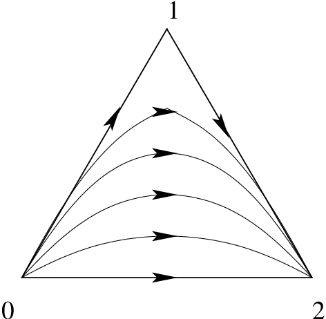
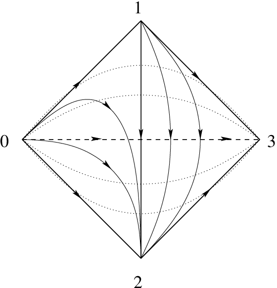
These are easily constructed by induction on $n$ using the elementary fact that $P_{0,n}\Delta^{n}$ is contractible. When $n=1$ , the unique point of $I^{0}$ goes to any path from $0$ to $1$ in $\Delta^{1}$ . The cases $n=2$ and 3 are illustrated in Figure 2.

For a pointed topological space $(X,x)$ , let $S^{(0)}_{\bullet}(X,x)$ be the subcomplex of the singular chain complex generated by those singular simplices $\sigma:\Delta^{n}\to X$ that map all vertices of $\Delta^{n}$ to $x$ . If $X$ is path connected, this computes the integral homology of $X$ .

For each such singular simplex $\sigma:\Delta^{n}\to X$ , we have the singular cube $P(\sigma)\circ\theta_{n}:I^{n-1}\to P_{x,x}X$ . Set

(17)

[\sigma]=\begin{cases}P(\sigma)\circ\theta_{n}-c_{x}&n=1;\cr P(\sigma)\circ\theta_{n}&n>1,\end{cases}

where $c_{x}$ denotes the constant loop at $x$ . Set¹⁷¹⁷ 17 Strictly speaking, we need to use Moore paths as we need path multiplication to be associative.

[\sigma_{1}|\sigma_{2}|\dots|\sigma_{s}]=[\sigma_{1}]\ast[\sigma_{2}]\ast\cdots\ast[\sigma_{n}]

This extends to an algebra mapping

	$\displaystyle\bigoplus_{s\geq 0}\big(S^{(0)}_{>0}(X,x)\big)^{\otimes s}$	$\displaystyle\to\{\text{reduced cubical chains on }P_{x,x}X\}$
	$\displaystyle\sigma_{1}\otimes\cdots\otimes\sigma_{s}$	$\displaystyle\mapsto[\sigma_{1}\|\cdots\|\sigma_{s}],$

which is easily seen be to injective. The formula (16) implies that

(18)

\partial[\sigma]=-[\partial\sigma]+\sum_{1\leq j<n}(-1)^{j}[\sigma_{(j)}|\sigma^{(n-j)}],

where $\sigma_{(j)}$ denotes the front $j$ face and $\sigma^{(n-j)}$ the rear $(n-j)$ th face of $\sigma$ .

Adams’ cobar construction is, by definition, the free associative algebra

\mathit{Ad}(S^{(0)}_{\bullet}(X,x))=\bigoplus_{s\geq 0}\big(S^{(0)}_{>0}(X,x)\big)^{\otimes s}

on $S^{(0)}_{\bullet}(X,x)$ with the differential (18), where $\sigma_{1}\otimes\dots\otimes\sigma_{s}$ has degree $-s+\sum\deg\sigma_{j}$ . This is an augmented, associative, dga, where the augmentation ideal is generated by the $[\sigma]$ . Adams’ main result may be stated by saying that the chain mapping

\mathit{Ad}(S^{(0)}_{\bullet}(X,x))\to\{\text{reduced cubical chains on }P_{x,x}X\}

is a quasi-isomorphism when $X$ is simply connected. Stallings’ result [53] for $H_{0}$ is more elementary.

Proposition 14.3.

If $X$ is path connected, then there are natural augmentation preserving algebra isomorphisms

H_{0}(\mathit{Ad}(S^{(0)}_{\bullet}(X,x)))\cong H_{0}(P_{x,x}X;{\mathbb{Z}})\cong{\mathbb{Z}}\pi_{1}(X,x).

Sketch of proof.

The second isomorphism follows directly from the definitions. We will show that $H_{0}(\mathit{Ad}(S^{(0)}_{\bullet}(X,x)))$ is isomorphic to ${\mathbb{Z}}\pi_{1}(X,x)$ . Let ${\mathrm{Simp}}_{\bullet}(X,x)$ denote the simplicial set whose $k$ -simplices consist of all singular simplices $\sigma:\Delta^{k}\to X$ that map all vertices of $\Delta^{n}$ to $x$ . After unraveling the definitions (17) and (18), we see that $H_{0}(\mathit{Ad}(S^{(0)}_{\bullet}(X,x)))$ is the algebra generated by the 1-simplices ${\mathrm{Simp}}_{1}(X,x)$ (augmented by taking the generator corresponding to each 1-simplex to 1) divided out by the ideal generated by $\sigma_{01}-\sigma_{02}+\sigma_{12}$ , where $\sigma\in{\mathrm{Simp}}_{2}(X,x)$ and $\sigma_{jk}$ is the singular 1-simplex obtained by restricting $\sigma$ to the edge $jk$ of $\Delta^{2}$ . It follows from van Kampen’s Theorem that $H_{0}(\mathit{Ad}(S^{(0)}_{\bullet}(X,x)))$ is naturally isomorphic to the integral group ring of the fundamental group of the geometric realization of ${\mathrm{Simp}}_{\bullet}(X,x)$ . The result follows as the tautological mapping $|{\mathrm{Simp}}_{\bullet}(X,x)|\to X$ is a weak homotopy equivalence. ∎

With the standard diagonal mapping

\Delta:S^{(0)}_{\bullet}(X,x)\to S^{(0)}_{\bullet}(X,x)\otimes S^{(0)}_{\bullet}(X,x),\quad\sigma\mapsto\sum_{0<j<\deg\sigma}\sigma_{(j)}\otimes\sigma^{(n-j)}

$S^{(0)}_{\bullet}(X,x)$ is a coassociative differential graded coalgebra. The cobar construction can be defined for any connected, coassociative dg coalgebra $C_{\bullet}$ . The homology analogue of the Eilenberg-Moore spectral sequence implies that if $C_{\bullet}\to S^{(0)}_{\bullet}(X,x)$ is a dg coalgebra quasi-isomorphism, then the induced mapping

H_{\bullet}(\mathit{Ad}(C_{\bullet}))\to H_{\bullet}(\mathit{Ad}(S^{(0)}_{\bullet}(X,x)))

is an isomorphism provided $H_{1}(X;{\mathbb{Q}})=0$ , and that

H_{0}(\mathit{Ad}(C_{\bullet}))/I^{s}\to H_{0}(\mathit{Ad}(S^{(0)}_{\bullet}(X,x)))/I^{s}

is an isomorphism for all $s$ in general.

Elements of $S^{\bullet}(P^{\bullet}_{x,x}X)$ can be evaluated on elements of $\mathit{Ad}(S^{(0)}_{\bullet}(X,x))$ to obtain a chain mapping

S^{\bullet}(P^{\bullet}_{x,x}X;R)\to\operatorname{Hom}(\mathit{Ad}(S^{(0)}_{\bullet}(X,x)),R).

which is a quasi-isomorphism for all coefficients $R$ as can be seen using the Eilenberg-Moore spectral sequence. Consequently, the integral structures on $H^{\bullet}(\mathit{Ch}^{\bullet}(P_{x,y}X))$ one obtains from from $S^{\bullet}(X^{\bullet};{\mathbb{Z}})$ and $\mathit{Ad}(S^{(0)}_{\bullet}(X,x))$ agree.

References

[1] J. F. Adams: On the cobar construction Proc. Nat. Acad. Sci. U.S.A. 42 (1956), 409–412.
[2] J.F. Adams: On the cobar construction, Colloque de topologie algébrique, Louvain, 1956, Georges Thone, Liège; Masson & Cie, Paris, 1957, 81–87.
[3] J.F. Adams, P. Hilton: On the chain algebra of a loop space, Comment. Math. Helv. 30 (1956), 305–330.
[4] K. Aomoto: Addition theorem of Abel type for hyper-logarithms, Nagoya Math. J. 88 (1982), 55–71.
[5] S. Archava: Arithmetic Hodge structures on homotopy groups and intersection of algebraic cycles, Thesis, UCLA, 1999.
[6] M. Asakura: Motives and algebraic de Rham cohomology, The arithmetic and geometry of algebraic cycles (Banff, AB, 1998), CRM Proc. Lecture Notes, 24 (2000), 133–154.
[7] A. Beilinson: Higher regulators and values of $L$ -functions of curves, Funktsional. Anal. i Prilozhen 14 (1980), 46–47.
[8] A. Beilinson, A. Levin: The elliptic polylogarithm, Motives (Seattle, WA, 1991), Proc. Sympos. Pure Math., 55, Part 2, Amer. Math. Soc., Providence, RI, 1994, 123–190.
[9] S. Bloch: Applications of the dilogarithm function in algebraic $K$ -theory and algebraic geometry, Proceedings of the International Symposium on Algebraic Geometry (Kyoto Univ., Kyoto, 1977), 103–114.
[10] A. Borel: Stable real cohomology of arithmetic groups, Ann. Sci. Ecole Norm. Sup. 7 (1974), 235–272.
[11] A. Bousfield, D. Kan: Homotopy limits, completions and localizations, Lecture Notes in Mathematics, Vol. 304, Springer-Verlag, 1972.
[12] J. Carlson: Extensions of mixed Hodge structures, Journés de Gómetrie Algb́rique d’Angers, Juillet 1979 Sijthoff & Noordhoff, Alphen aan den Rijn, 1980, 107–127.
[13] J. Carlson, C. H. Clemmens, J. Morgan: On the mixed Hodge structure associated to $\pi_{3}$ of a simply connected complex projective manifold, Ann. Sci. École Norm. Sup. (4) 14 (1981), 323–338.
[14] K.-T. Chen: Iterated integrals, fundamental groups and covering spaces, Trans. Amer. Math. Soc. 206 (1975), 83–98.
[15] K.-T. Chen: Iterated path integrals, Bull. Amer. Math. Soc. 83 (1977),831–879.
[16] K.-T. Chen: Reduced bar constructions on de Rham complexes, Algebra, topology, and category theory (a collection of papers in honor of Samuel Eilenberg), Academic Press, New York, 1976, 19–32.
[17] K. T. Chen: Circular bar construction, J. Algebra 57 (1979), 446–483.
[18] A. Collino: Griffiths’ infinitesimal invariant and higher $K$ -theory on hyperelliptic Jacobians, J. Algebraic Geom. (1997), 393–415.
[19] E. Colombo: The mixed Hodge structure on the fundamental group of a hyperelliptic curve and higher cycles, preprint, 2000.
[20] M. Cushman: Morphisms of curves and the fundamental group, this volume.
[21] P. Deligne: Équations diffŕentielles à points singuliers réguliers, Lecture Notes in Mathematics, Vol. 163, Springer-Verlag, 1970.
[22] P. Deligne: Le groupe fondamental de la droite projective moins trois points, Galois groups over ${\mathbb{Q}}$ (Berkeley, CA, 1987), Math. Sci. Res. Inst. Publ. 16, Springer, New York, 1989, 79–297.
[23] V. Drinfeld: On quasitriangular quasi-Hopf algebras and on a group that is closely connected with ${\rm Gal}(\overline{{\mathbb{Q}}}/{\mathbb{Q}})$ , Algebra i Analiz 2 (1990), 149–181; translation in Leningrad Math. J. 2 (1991), 829–860.
[24] S. Eilenberg, J. Moore: Homology and fibrations, I: Coalgebras, cotensor product and its derived functors, Comment. Math. Helv. 40 (1966), 199–236.
[25] A. Goncharov: Geometry of configurations, polylogarithms, and motivic cohomology, Adv. Math. 114 (1995), 197–318.
[26] M. Green, P. Griffiths: Unpublished manuscripts.
[27] A. Grothendieck: On the de Rham cohomology of algebraic varieties, Inst. Hautes Études Sci. Publ. Math. No. 29 (1966), 95–103.
[28] R. Hain: Iterated integrals, intersection theory and link groups, Topology 24 (1985), 45–66. Erratum: Topology 25 (1986), 585–586.
[29] R. Hain: On the indecomposable elements of the bar construction, Proc. Amer. Math. Soc. 98 (1986), 312–316.
[30] R. Hain: The de Rham homotopy theory of complex algebraic varieties, I and II, $K$ -Theory 1 (1987), 271–324 and 481–497.
[31] R. Hain: Iterated integrals and mixed Hodge structures on homotopy groups, Hodge theory (Sant Cugat, 1985), Lecture Notes in Math., 1246, Springer, Berlin, 1987, 75–83.
[32] R. Hain: Higher albanese manifolds, Hodge theory (Sant Cugat, 1985), Lecture Notes in Math., 1246, Springer, Berlin, 1987, 84–91.
[33] R. Hain: The geometry of the mixed Hodge structure on the fundamental group, Algebraic geometry, Bowdoin, 1985 (Brunswick, Maine, 1985), Proc. Sympos. Pure Math., 46, Part 2, Amer. Math. Soc., Providence, RI, 1987, 247–282.
[34] R. Hain: Classical polylogarithms, Motives (Seattle, WA, 1991), Proc. Sympos. Pure Math., 55, Part 2, Amer. Math. Soc., Providence, RI, 1994, 3–42.
[35] R. Hain: The Hodge de Rham theory of relative Malcev completion, Ann. Sci. École Norm. Sup. (4) 31 (1998), 47–92.
[36] R. Hain: Infinitesimal presentations of the Torelli groups, J. Amer. Math. Soc. 10 (1997), 597–651.
[37] R. Hain, R. MacPherson: Higher logarithms, Illinois J. Math. 34 (1990), 392–475.
[38] R. Hain, J. Yang: Real Grassmann polylogarithms and Chern classes Math. Ann. 304 (1996), 157–201.
[39] R. Hain, S. Zucker: Unipotent variations of mixed Hodge structure, Invent. Math. 88 (1987), 83–124.
[40] B. Harris: Harmonic volumes, Acta Math. 150 (1983), 91–123.
[41] Hochschild, G. Mostow: Pro-affine algebraic groups, Amer. J. Math. 91 (1969), 1127–1140.
[42] H. Kim, R. Hain: A De Rham-Witt approach to crystalline rational homotopy theory, math.AG/0105008.
[43] J. King: The currents defined by analytic varieties, Acta Math. 127 (1971), 185–220.
[44] J. King: Log complexes of currents and functorial properties of the Abel-Jacobi map, Duke Math. J. 50 (1983), 1–53.
[45] M. Kontsevich: Vassiliev’s knot invariants, I.M. Gel’fand Seminar, 137–150, Adv. Soviet Math., 16, Part 2, Amer. Math. Soc., Providence, RI, 1993.
[46] C. Miller: Exponential iterated integrals and the solvable completion of fundamental groups, Senior Thesis, Duke University, 2001.
[47] J. Milnor, J. Moore: On the structure of Hopf algebras, Ann. of Math. 81 (1965), 211–264.
[48] J. Morgan: The algebraic topology of smooth algebraic varieties, Inst. Hautes Études Sci. Publ. Math. No. 48 (1978), 137–204; Correction: Inst. Hautes Études Sci. Publ. Math. No. 64 (1986), 185.
[49] V. Navarro Aznar: Sur la thórie de Hodge-Deligne, Invent. Math. 90 (1987), 11–76.
[50] M. Pulte: The fundamental group of a Riemann surface: mixed Hodge structures and algebraic cycles, Duke Math. J. 57 (1988), 721–760.
[51] A. Shiho: Crystalline fundamental groups and $p$ -adic Hodge theory, The arithmetic and geometry of algebraic cycles (Banff, AB, 1998), CRM Proc. Lecture Notes, 24, Amer. Math. Soc., Providence, RI, 2000, 381–398.
[52] D. Quillen: Rational homotopy theory, Ann. of Math. 90 (1969), 205–295.
[53] J. Stallings: Quotients of the powers of the augmentation ideal in a group ring, in Knots, groups, and $3$ -manifolds (Papers dedicated to the memory of R.H. Fox), Ann. of Math. Studies, No. 84, Princeton Univ. Press, 1975, 101–118.
[54] D. Sullivan: Infinitesimal computations in topology, Inst. Hautes Études Sci. Publ. Math. No. 47 (1977), 269–331
[55] T. Terasoma: Mixed Tate motives and multiple zeta values, math.AG/0104231.
[56] J.H.C. Whitehead: An expression of Hopf’s invariant as an integral, Proc. Nat. Acad. Sci U. S. A. 33, (1947), 117–123.
[57] Z. Wojtkowiak: Cosimplicial objects in algebraic geometry, Algebraic $K$ -theory and algebraic topology (Lake Louise, AB, 1991), NATO Adv. Sci. Inst. Ser. C Math. Phys. Sci., 407, Kluwer Acad. Publ., Dordrecht, 1993, 287–327.
[58] J. Yang: Algebraic $K$ -groups of number fields and the Hain-MacPherson trilogarithm, Ph.D. thesis, University of Washington, 1991.
[59] D. Zagier: Values of zeta functions and their applications, First European Congress of Mathematics, Vol. II (Paris, 1992), 497–512, Progr. Math., 120, Birkhäuser, Basel, 1994.
[60] J. Zhao: Multiple polylogarithms: analytic continuation, monodromy, and variations of mixed Hodge structure, this volume.

	$\displaystyle m[dg\|a_{1}\|\dots\|a_{r}]n$	$\displaystyle=m[ga_{1}\|\dots\|a_{r}]n-m\cdot g[a_{1}\|\dots\|a_{r}]n;$
	$\displaystyle\begin{split}m[a_{1}\|\dots\|a_{i}\|dg\|a_{i+1}\|\dots\|a_{r}]n&=m[a_{1}\|\dots\|a_{i}\|g\,a_{i+1}\|\dots\|a_{r}]n\cr&\qquad-m[a_{1}\|\dots\|a_{i}\,g\|a_{i+1}\|\dots\|a_{r}]n\quad 1\leq i<s;\end{split}$
	$\displaystyle m[a_{1}\|\dots\|a_{r}\|dg]n$	$\displaystyle=m[a_{1}\|\dots\|a_{r}]g\cdot n-m[a_{1}\|\dots\|a_{r}\,g]n;$
	$\displaystyle m[dg]n$	$\displaystyle=1\otimes g\cdot n-m\cdot g\otimes 1$