跳到论文正文
W Papers独立论文阅读器 arXiv:math/0108153 论文正文 计算阅读时间 · 0%
引用这篇论文根据当前论文元数据生成,正式投稿前建议核对。


License: arXiv.org perpetual non-exclusive license
arXiv:math/0108153v2 [math.GT] 19 Mar 2009

On graphical foliations and the global existence of Euler’s multiplier

Marco Kühnel Michael Neudert Department of Mathematics Department of Mathematics Otto-von-Guericke-University Magdeburg University of Bayreuth P.O. Box 4120 D-95440 Bayreuth D-39016 Magdeburg Note: The author gratefully acknowledges support by the DFG-priority program “Global Methods in Complex Geometry”.
Abstract

We present a criterion for the global existence of Euler’s multiplier for an integrable one-form taking into account the corresponding codim-1-foliation. In particular, the impact of inseparable leaves is considered. Here, we suppose that the foliation can be reduced to a graph. The properties of this graph are crucial for the global existence of the Euler’s multiplier. As applications we investigate some special cases in which the graph turns out to look very simple.

1 Introduction

First order differential equations of the form

(1) g⁡(x,y)​d​x+h⁡(x,y)​d​y=0g(x,y)dx+h(x,y)dy=0

sometimes can be transformed to exact differential equations and be solved by finding a so called integrating factor, i.e. some function λ=λ⁡(x,y)≠0\lambda=\lambda(x,y)\not=0 such that there is some function f=f⁡(x,y)f=f(x,y) with the property

d​f=λ​g​d​x+λ​h​d​y.df\ =\ \lambda\ g\ dx+\lambda\ h\ dy.

In general, λ\lambda is supposed to vanish nowhere or, at least, in a set with no interior points (see [Ma94]). Then ff is a first integral of equation (1) and the solutions are implicitly given by the equation f⁡(x,y)=const.f(x,y)=\mbox{\rm const}. It is well known that, if |g⁡(x0,y0)|+|h⁡(x0,y0)|>0|g(x_{0},y_{0})|+|h(x_{0},y_{0})|>0, there are some neighbourhood UU of (x0,y0)(x_{0},y_{0}) and nontrivial functions λ,f:U→ℝ\lambda,f:U\to{\mathbb{R}} as above.
In higher dimensions, the situation is more complicated. Let r∈ℕr\in{\mathbb{N}}, r≥1r\geq 1, and MM be a real CrC^{r} manifold of dimension n+1n+1 and ω\omega a CrC^{r} one-form on MM. In this article we assume a manifold to be second countable, i.e. it has a countable topological base. This implies that it is paracompact, hence metrizable, and can be covered by a countable number of charts. Now we ask for the existence of functions f∈Cr​(M,ℝ)f\in C^{r}(M,{\mathbb{R}}), λ∈Cr−1​(M,ℝ)\lambda\in C^{r-1}(M,{\mathbb{R}}) such that λ⁡(x)≠0\lambda(x)\not=0 and

d​f=λ​ωdf=\lambda\omega

in MM. In this case, λ\lambda is called Euler’s multiplier. From d⁡(d​f)=0d(df)=0 follows immediately that

(2) ω∧d​ω= 0\omega\land d\omega\ =\ 0

is a necessary condition for the existence of such functions λ\lambda and ff. In this case ω\omega is called an integrable one-form. From Frobenius’ theorem one can derive the local existence of λ\lambda and ff in a neighbourhood of p∈Mp\in M if condition (2) is satisfied and ω⁡(p)≠0\omega(p)\not=0 (see e.g. [vWe]). But even if these conditions are satisfied everywhere in MM and MM is simply connected, global existence is, in general, not guaranteed. Consider the following example: Let M=ℝ3M={\mathbb{R}}^{3}, represented in cylinder coordinates (ϱ,ϕ,z)∈[0,∞)×[0,2​π)×ℝ(\varrho,\phi,z)\in\ [0,\infty)\times[0,2\pi)\times{\mathbb{R}}, wϱ:=ϱ2\ w_{\varrho}:=\varrho^{2},

wϕ:={0,0≤ϱ<124​(ϱ−12)2​(ϱ−1),12≤ϱ<1ϱ−1,1≤ϱwz:={(14−ϱ2)2,0≤ϱ<120,12≤ϱ{w_{\phi}:=\begin{cases}0,&0\leq\varrho<\frac{1}{2}\\ 4(\varrho-\frac{1}{2})^{2}(\varrho-1),&\frac{1}{2}\leq\varrho<1\\ \varrho-1,&1\leq\varrho\end{cases}}\quad\quad{w_{z}:=\begin{cases}(\frac{1}{4}-\varrho^{2})^{2},&0\leq\varrho<\frac{1}{2}\\ 0,&\frac{1}{2}\leq\varrho\end{cases}}

ω=wϱ​d​ϱ+wϕ​d​ϕ+wz​d​z.\omega=w_{\varrho}d\varrho+w_{\phi}d\phi+w_{z}dz.

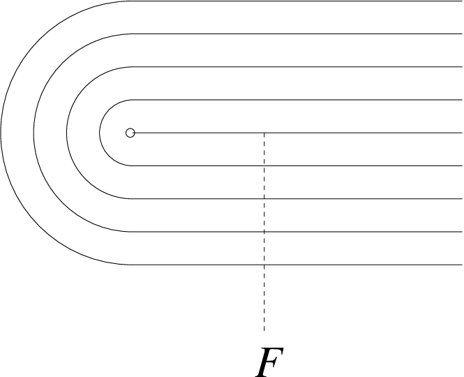
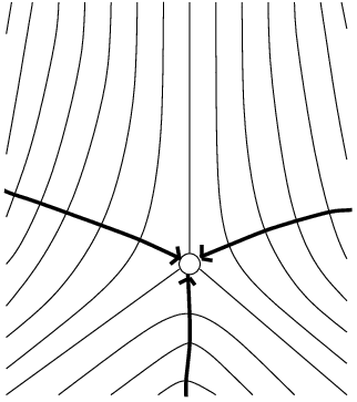
Obviously, ω\omega vanishes nowhere and condition (2) is satisfied. But in any neighbourhood of {ϱ=1}\{\varrho=1\} Euler’s multiplier cannot exist. Here, the geometry of those manifolds FF, which are locally the level sets of a function ff, forbid the existence of ff and λ\lambda since they wind around the cylinder {ϱ=1}\{\varrho=1\} (see Fig. 1).

Refer to caption
Figure 1:

As we can deduce from this example, the geometry of these manifolds, which, in general, cannot be represented as submanifolds of MM and which we will call leaves, has a decisive impact on the existence of λ\lambda and ff.

The geometric term useful in this context is the codim-1-foliation induced by an integrable one-form (see §\lx@sectionsign2). Obviously, in case of global existence of λ\lambda and ff, all these leaves are closed subsets of MM. Moreover, it turns out that the holonomy group (see §\lx@sectionsign2) has to be trivial.

The first question is, whether those two conditions are sufficient for the global existence of Euler’s multiplier. It turns out that this is only right if we additionally assume the leaves to be compact.

In general, to find a sufficient criterion for global existence, the differentiable structure of M/ℱM/{\cal F} is decisive. In M/ℱM/{\cal F}, points of MM lying on the same leaf are identified, in other words, M/ℱM/{\cal F} is the space of leaves. In general, the topology in M/ℱM/{\cal F} induced by the canonical projection π:M→M/ℱ\pi:M\to M/{\cal F} is non-Hausdorff.

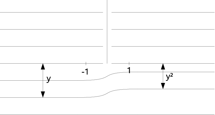
Note that for non-Hausdorff one-dimensional manifolds homeomorphic classes are different form diffeomorphic classes. So, if we only use topological properties of M/ℱM/{\cal F} we cannot expect the full regularity of Euler’s multiplier. In order to get a CrC^{r} multiplier we have to assume an additional property of ℱ{\cal F} involving the differentiable structure. We call this property regularly CrC^{r}. The following example will shed some light on it:


By construction, any C1C^{1} function ff constant on the leaves would satisfy f⁡(x,y)=f⁡(−x,−y2)f(x,y)=f(-x,-y^{2}), if x<−1x<-1 and y<0y<0. Hence ∂f∂y​(x,0)=0\frac{\partial f}{\partial y}(x,0)=0, if x<−1x<-1. So d​f​(x,0)=0df(x,0)=0. This prevents the existence of Euler’s multiplier although the topological structure is admissible (compare §\lx@sectionsign 5).

Refer to caption
Figure 2: An irregular foliation on the slit plane

On the other hand, for Hausdorff one-dimensional manifolds there is no difference between homeomorphic classes and diffeomorphic classes. So, if we can prove M/ℱ≅ℝM/{\cal F}\cong{\mathbb{R}} in the topological sense, this will be enough to have Euler’s multiplier.

In order to reduce M/ℱM/{\cal F} to its relevant topological properties, the terminology and the theory of graphs turn out to be appropriate means. More precisely, the structure of M/ℱM/{\cal F} will be displayed by a configuration of graphs. Here, the so called inseparable or non-Hausdorff leaves, i.e. leaves that cannot be separated in the topology of M/ℱM/{\cal F} play an important part. They determine essentially the structure of the graphs. The construction of the corresponding graphs is possible under some weak assumptions on the foliation ℱ{\cal F} (cf. Def. 5.1). This leads us in a natural way to the concept of the graphical configuration induced by a codim-1-foliation (see §\lx@sectionsign4), which finally yields an equivalent criterion for the global existence of Euler’s multiplier.

In particular, we are able to give a ’classification’ of obstructions for the global existence of Euler’s multiplier, all but one can be expressed in terms of the topology of M/ℱM/{\cal F}: (1.) non-regularity of ℱ{\cal F}, (2.) there is at least one non-closed point in M/ℱM/{\cal F}, (3.) there is too much ramification in M/ℱM/{\cal F}, (4.) there are other obstructions coming from the local topology of M/ℱM/{\cal F} or (5.) obstructions coming from the global topology of M/ℱM/{\cal F}.

For an example for (3.) on M=ℝ2M={\mathbb{R}}^{2} we refer to [CN, Ch. III, Notes] (found by Wazewski) or [H76].

The authors would like to express their gratitude to Wolf von Wahl for initiating this project.

2 Foliations and one-forms

2.1 Foliations

Let MM be a real CrC^{r} manifold of dimension NN. A maximal CrC^{r} atlas ℱ=(Uι,φι)ι∈𝒥{\cal F}=(U_{\iota},\varphi_{\iota})_{\iota\in{\cal J}} of MM is called a codim-kk-foliation if and only if

  1. (a)

    For each ι∈𝒥\iota\in{\cal J} there exist open disks Xι∈ℝN−k,Yι∈ℝkX_{\iota}\in{\mathbb{R}}^{N-k},Y_{\iota}\in{\mathbb{R}}^{k} such that

    φι​(Uι)=Xι×Yι,\varphi_{\iota}(U_{\iota})=X_{\iota}\times Y_{\iota},
  2. (b)

    if (Uι1,φι1),(Uι2,φι2)∈ℱ(U_{\iota_{1}},\varphi_{\iota_{1}}),(U_{\iota_{2}},\varphi_{\iota_{2}})\in{\cal F} with Uι1∩Uι2≠∅\ U_{\iota_{1}}\cap U_{\iota_{2}}\not=\emptyset\ then the mapping

    φι2∘φι1−1:φι1​(Uι1∩Uι2)→φι2​(Uι1∩Uι2)\varphi_{\iota_{2}}\circ\varphi_{\iota_{1}}^{-1}:\ \varphi_{\iota_{1}}(U_{\iota_{1}}\cap U_{\iota_{2}})\to\varphi_{\iota_{2}}(U_{\iota_{1}}\cap U_{\iota_{2}})

    is of the form

    (φι2∘φι1−1)​(x,y)=(ϕι1​ι2​(x,y),ψι1​ι2​(y)).\bigl(\varphi_{\iota_{2}}\circ\varphi_{\iota_{1}}^{-1}\bigr)(x,y)\ =\ \bigl(\phi_{\iota_{1}\iota_{2}}(x,y),\psi_{\iota_{1}\iota_{2}}(y)\bigr).

The charts (Uι,φι)(U_{\iota},\varphi_{\iota}) are called foliation charts. The leaves FF of ℱ{\cal F} are defined as follows: Fix any point p∈Uι0⊂Mp\in U_{\iota_{0}}\subset M. For any point q∈Mq\in M we will say q∈Fpq\in F_{p} if and only if there exists a finite sequence (ιμ)μ=0,…,m⊂𝒥(\iota_{\mu})_{\mu=0,...,m}\subset{\cal J} and cι0∈Yι0,…,cιm∈Yιmc_{\iota_{0}}\in Y_{\iota_{0}},...,c_{\iota_{m}}\in Y_{\iota_{m}} such that

  1. (a)

    Uιμ−1∩Uιμ≠∅U_{\iota_{\mu-1}}\cap U_{\iota_{\mu}}\not=\emptyset, μ=1,…,m\ \mu=1,...,m,

  2. (b)

    φιμ−1−1​(Xιμ−1×{cιμ−1})∩φιμ−1​(Xιμ×{cιμ})≠∅\varphi_{\iota_{\mu-1}}^{-1}\bigl(X_{\iota_{\mu-1}}\times\{c_{\iota_{\mu-1}}\}\bigr)\cap\varphi_{\iota_{\mu}}^{-1}\bigl(X_{\iota_{\mu}}\times\{c_{\iota_{\mu}}\}\bigr)\not=\emptyset, μ=1,…,m\ \mu=1,...,m,

  3. (c)

    p∈φι0−1​(Xι0×{cι0})p\in\varphi_{\iota_{0}}^{-1}\bigl(X_{\iota_{0}}\times\{c_{\iota_{0}}\}\bigr), q∈φιm−1​(Xιm×{cιm})\ q\in\varphi_{\iota_{m}}^{-1}\bigl(X_{\iota_{m}}\times\{c_{\iota_{m}}\}\bigr)

It is clear, that by p​∼ℱ​q​ :⟺q∈Fpp\overset{\cal F}{\sim}q\mbox{\hskip 2.84526pt}:\Longleftrightarrow q\in F_{p} an equivalence relation is defined. Any equivalence class F=Fp=[p]∼ℱF=F_{p}=[p]_{\overset{\cal F}{\sim}}, pp∈\inMM, will be called a leaf of ℱ{\cal F}.
The space of leaves is denoted by M/ℱ:=M/ℱ∼M/{\cal F}:=M/{\underset{\mbox{\large$\sim$}}{\mbox{\tiny${\cal F}$}}}, and π:M→M/ℱ,p↦Fp\pi:M\to M/{\cal F},p\mapsto F_{p} is the canonical projection. In this article, we consider M/ℱM/{\cal F} as a topological space endowed with the topology induced by π\pi. The projection π\pi then becomes a continuous and open mapping.
In what follows, for any leaf FF of ℱ{\cal F} we will write F∈M/ℱF\in M/{\cal F} if we consider FF as a point in M/ℱM/{\cal F} and, deviating from the exact definition of the foliation, F∈ℱF\in{\cal F} if FF is considered as a subset of MM.
At this occasion, we point out that, of course, the sets φι−1​(Xι×{c})\varphi_{\iota}^{-1}\bigl(X_{\iota}\times\{c\}\bigr), c∈Yιc\in Y_{\iota}, are submanifolds of dimension NN−-kk, but in general the leaves F∈ℱF\in\cal F are not necessarily submanifolds; they are immersed manifolds. For this and other theorems in the theory of foliations used in this article we refer to [CN].
For any subset U⊂MU\subset M we define the saturation of UU with respect to ℱ{\cal F} by sat⁡(U):=π−1​(π⁡(U)){\rm sat}\ (U):=\pi^{-1}\bigl(\pi(U)\bigr). Any subset U⊂MU\subset M is called saturated (with respect to ℱ{\cal F}) if and only if sat⁡(U)=U{\rm sat}\ (U)=U, i.e., for each p∈Up\in U holds Fp⊂UF_{p}\subset U.

We call the foliation transversely orientable, if the normal bundle given by Nℱ,x:=Tx​M/Tx​FxN_{{\cal F},x}:=T_{x}M/T_{x}F_{x} is orientable. The transversely orientable codim-1-foliations are exactly those given by integrable one-forms.

2.2 The holonomy group

We now give a short sketch of the construction of holonomy. Fix a leaf FF and a point p∈Fp\in F. Now consider a closed path γ:[0;2​π]⟶F\gamma:[0;2\pi]\longrightarrow F with γ⁡(0)=γ⁡(2​π)=p\gamma(0)=\gamma(2\pi)=p. Now, if we choose a local transversal TT through pp and cover γ⁡([0;2​π])\gamma([0;2\pi]) by a finite number of foliation charts (Uι,φι)ι=1,…,k(U_{\iota},\varphi_{\iota})_{\iota=1,...,k}, we can choose points pi∈γ⁡([0;2​π])p_{i}\in\gamma([0;2\pi]) and local transversals TiT_{i} through pip_{i} such that Ti∪Ti+1⊂UιT_{i}\cup T_{i+1}\subset U_{\iota} for a ι∈{1,…,k}\iota\in\{1,...,k\}. By going into the foliation charts we are now able to choose a path γt:[0;2​π]⟶Ft\gamma_{t}:[0;2\pi]\longrightarrow F_{t} for a t∈Tt\in T sufficiently near to pp, which intersects each TiT_{i}.

Indeed, it can be shown, that γt​(2​π)\gamma_{t}(2\pi) is independent of the choices of pip_{i}, TiT_{i} and the chosen paths γt\gamma_{t}. Moreover, γt​(2​π)\gamma_{t}(2\pi) only depends on the homotopy class of γ\gamma. Hence we get a map

h:π1​(F,p)⟶Aut⁡(T,p),h:\pi_{1}(F,p)\longrightarrow{\rm Aut}(T,p),

where π1​(F,p)\pi_{1}(F,p) is the fundamental group of FF with respect to pp and Aut⁡(T,p){\rm Aut}(T,p) denotes the germs of automorphisms of TT which fix pp. We call

Hol​(F,p):=h⁡(π1​(F,p))\mbox{\rm Hol}(F,p):=h\bigl(\pi_{1}(F,p)\bigr)

the holonomy of the leaf FF. Indeed, Hol​(F,p)\mbox{\rm Hol}(F,p) is independent of the base point pp, so that we will denote this by Hol​(F)\mbox{\rm Hol}(F). For more details of the construction we refer to [CN].

2.3 The foliation of an integrable one-form

Let MM be a real manifold of dimension nn++11, ω\omega a CrC^{r} one-form on MM. Thus, for each p∈Mp\in M

ω⁡(p):Tp​M→ℝ\omega(p):\quad T_{p}M\to{\mathbb{R}}

is a linear mapping. Setting

P⁡(p):=ker​ω​(p),P(p):={\rm ker}\ \omega(p),

where ω⁡(p)≠0\omega(p)\not=0, an nn-plane field PP is defined on MM.
Frobenius’ Theorem yields that PP is induced by a codim-1-foliation on MM if and only if PP is completely integrable, which is equivalent to the condition

ω∧d​ω=0\omega\wedge d\omega=0

on MM (see [CN, Ch.II §\lx@sectionsign 4, Appendix §\lx@sectionsign 3 Th.2]).
Thus, each completely integrable CrC^{r} one-form ω\omega on MM with ω⁡(p)≠0\omega(p)\not=0 in MM induces a CrC^{r} codim-1-foliation ℱ=ℱ⁡(ω){\cal F}={\cal F}(\omega) on MM, where for p∈Fp\in F, F∈ℱF\in{\cal F}

Tp​F​ = ​ker​ω​(p).T_{p}F\mbox{\hskip 2.84526pt}=\mbox{\hskip 2.84526pt}{\rm ker}\ \omega(p).

Now, considering the corresponding foliation charts of MM, the local existence of Euler’s multiplier is clear.

Moreover, the global existence of Euler’s multiplier easily implies that Hol​(F)={1}\mbox{\rm Hol}(F)=\{1\} for all leaves FF.

Also note that the foliation given by an integrable, nowhere vanishing one-form ω\omega is transversely orientable: By using a partition of unity one can easily construct a CrC^{r} vector field XX satisfying ω⁡(X)≡1\omega(X)\equiv 1.

Finally, we want to mention the Godbillon-Vey class of ℱ⁡(ω){\cal F}(\omega) (see [GV71]), if r≥dimM≥3r\geq\dim M\geq 3. Since ω∧d​ω=0\omega\wedge d\omega=0, we can find a one-form η\eta such that d​ω=ω∧ηd\omega=\omega\wedge\eta. Now the Godbillon-Vey class is defined

g​v​(ω):=[−η∧d​η]∈H3​(M,ℝ)gv(\omega):=[-\eta\wedge d\eta]\in H^{3}(M,{\mathbb{R}})

as a de Rham class. Taking the cohomological class instead of the form itself has the effect, that g​v​(ω)=g​v​(f​ω)gv(\omega)=gv(f\omega) for any non-vanishing f∈Cr​(M)f\in C^{r}(M). So it depends only on the foliation, not on the one-form. If ω\omega allows for Euler’s multiplier, g​v​(ω)=0gv(\omega)=0.

3 Transverse fibrations

For the sake of simplicity, in this section all manifolds and maps are considered to be C∞C^{\infty} unless stated otherwise. A fibre bundle ϕ:M⟶B\phi:M\longrightarrow B with M,BM,B being manifolds is called transverse to the foliation ℱ{\cal F} on MM, if and only if

ϕ|F:F⟶B\phi|F:F\longrightarrow B

is an unramified, surjective covering map for every leaf FF and therefore, in particular,

Tp​M=Tp​F⊕Tp​Mϕ⁡(p),T_{p}M=T_{p}F\oplus T_{p}M_{\phi(p)},

where p∈Fp\in F and Mϕ⁡(p):=ϕ−1​(ϕ⁡(p))M_{\phi(p)}:=\phi^{-1}(\phi(p)) is the fibre of ϕ\phi over ϕ⁡(p)\phi(p). In this situation we will also say, that ℱ{\cal F} is transverse to ϕ\phi. In our context, we assume, that dimM=n+1\dim M=n+1 and dimB=n\dim B=n and hence, that ℱ{\cal F} is a codimension one foliation.

For such ϕ\phi we can define a global version of holonomy in the following way. Given a closed path α:[0;2​π]⟶B\alpha:[0;2\pi]\longrightarrow B on BB and a point y∈ϕ−1​(α⁡(0)):=Ty\in\phi^{-1}(\alpha(0)):=T, we can look at the lifting α~:[0;2​π]⟶Fy\tilde{\alpha}:[0;2\pi]\longrightarrow F_{y} on the leaf FyF_{y} containing yy with α~​(0)=y\tilde{\alpha}(0)=y. Mapping y↦α~​(2​π)y\mapsto\tilde{\alpha}(2\pi) induces a CrC^{r} diffeomorphism ϕα:T⟶T\phi_{\alpha}:T\longrightarrow T. In fact, ϕα\phi_{\alpha} only depends on the homotopy class of α\alpha. So we get a representation

𝒉:π1​(B)⟶Diffr​(T),{\boldsymbol{h}}:\pi_{1}(B)\longrightarrow\mbox{\rm Diff}^{r}(T),

where π1​(B)\pi_{1}(B) is the fundamental group of BB and Diffr​(T)\mbox{\rm Diff}^{r}(T) the group of CrC^{r} automorphisms of TT. We call the image of 𝒉{\boldsymbol{h}} the global holonomy group (with respect to ϕ\phi) of ℱ{\cal F} and denote this by Hol​(ℱ/B)\mbox{\rm Hol}({\cal F}/B). For details see again [CN].

As ϕ|F:F⟶B\phi|F:F\longrightarrow B is a covering map, we can embed π1​(F)⊂π1​(B)\pi_{1}(F)\subset\pi_{1}(B) and look at the restricted map

𝒉|F:π1​(F)⟶Diffr​(T),{\boldsymbol{h}}|F:\pi_{1}(F)\longrightarrow\mbox{\rm Diff}^{r}(T),

whose image we call Hol~​(F)\widetilde{\mbox{\rm Hol}}(F), on the one hand and at the ordinary holonomy map

hF:π1​(F)⟶Hol​(F)h_{F}:\pi_{1}(F)\longrightarrow\mbox{\rm Hol}(F)

on the other hand, both of them are group homomorphisms. By definition of 𝒉{\boldsymbol{h}} follows that

ker​(𝒉|F)⊂ker​(hF)\mbox{ker}({\boldsymbol{h}}|F)\subset\mbox{ker}(h_{F})

and hence there is a surjective homomorphism

Hol~​(F)=π1​(F)/ker​(𝒉|F)⟶π1​(F)/ker​(hF)=Hol​(F).\widetilde{\mbox{\rm Hol}}(F)=\pi_{1}(F)/\mbox{ker}({\boldsymbol{h}}|F)\longrightarrow\pi_{1}(F)/\mbox{ker}(h_{F})=\mbox{\rm Hol}(F)\hskip-8.61108pt.

We now proved that Hol​(F)\mbox{\rm Hol}(F) is a quotient of a subgroup of Hol​(ℱ/B)\mbox{\rm Hol}({\cal F}/B) for every leaf FF.

So Hol​(ℱ/B)=1\mbox{\rm Hol}({\cal F}/B)=1 implies Hol​(F)=1\mbox{\rm Hol}(F)=1 for all leaves FF, but the converse is not true.

Theorem 3.1

Let ϕ:M⟶B\phi:M\longrightarrow B a fibre bundle and ℱ{\cal F} a transverse codim-1-foliation, both of class CrC^{r}. Then are equivalent:

  1. (a)

    There is a CrC^{r} function f:M⟶ℝf:M\longrightarrow{{\mathbb{R}}} such that d​f​(x)≠0df(x)\not=0 in MM and ℱ=ℱ⁡(d​f){\cal F}={\cal F}(df).

  2. (b)

    Hol​(ℱ/B)=1\mbox{\rm Hol}({\cal F}/B)=1 and the fibres of ϕ\phi are diffeomorphic to ℝ{{\mathbb{R}}}.

In particular, M≅B×ℝM\cong B\times{{\mathbb{R}}} if one (and hence both) of the conditions is satisfied.

Proof:  ’⇒\Rightarrow’: Let FF be a leaf and TT a fibre of ϕ\phi, meeting in a point p∈Mp\in M. Then we obtain a non-vanishing vector field XX along TT satisfying

d​f|T​(X)>0.df|_{T}(X)>0\hskip-8.61108pt.

Now let γ:[0,y]⟶T\gamma:[0,y]\longrightarrow T be a differentiable path in TT such that

d​γ​(t)​(1)=X⁡(γ⁡(t)),d\gamma(t)(1)=X(\gamma(t)),

By Stokes’ Theorem f⁡(γ⁡(y))−f⁡(γ⁡(0))>0f(\gamma(y))-f(\gamma(0))>0. So TT is diffeomorphic to ℝ{{\mathbb{R}}} and intersects each leaf exactly once. This implies Hol​(ℱ/B)=1\mbox{\rm Hol}({\cal F}/B)=1, in particular.

’⇐\Leftarrow’: Let TT be a fibre of ϕ\phi. The condition Hol​(ℱ/B)=1\mbox{\rm Hol}({\cal F}/B)=1 implies that TT intersects each leaf FF in exactly one point. This means that there is a differentiable map ψ:M⟶T\psi:M\longrightarrow T. Now take a diffeomorphism δ:T⟶ℝ\delta:T\longrightarrow{{\mathbb{R}}} and define f:=δ∘ψf:=\delta\circ\psi. Then the leaves of ℱ{\cal F} are the level sets of ff. The construction easily yields d​f​(x)≠0df(x)\not=0 everywhere. □\square

Let us recall that the relative tangent bundle TM|BT_{M|B} is defined by

TM|B,x=d​ix​(Tx​Mϕ⁡(x)),T_{M|B,x}=di_{x}(T_{x}M_{\phi(x)}),

where Mϕ⁡(x)M_{\phi(x)} is again the fibre over ϕ⁡(x)\phi(x), i:Mϕ⁡(x)⟶Mi:M_{\phi(x)}\longrightarrow M the natural embedding and d​ixdi_{x} the derivative of ii at xx, embedding the tangent bundle of the fibre into the tangent bundle of MM. The ii-th Betti number of a manifold BB is denoted by bi​(B)=dimHi​(B,ℝ)b_{i}(B)=\dim H^{i}(B,{\mathbb{R}}).

Definition 3.2

Let MM be a manifold and ϕ:M⟶B\phi:M\longrightarrow B a fibre bundle. We call MM ϕ\phi-orientable if and only if TM|BT_{M|B} is orientable.

Theorem 3.3

Let M,BM,B be manifolds, ϕ:M⟶B\phi:M\longrightarrow B a fibre bundle such that dimM=dimB+1\dim M=\dim B+1 and MM is ϕ\phi-orientable. If b2​(B)=0b_{2}(B)=0, then there is a transverse and transversely orientable foliation ℱ{\cal F} and a Riemannian metric on MM such that TM|B=Tℱ⟂T_{M|B}=T_{\cal F}^{\perp} and all fibres of π\pi are geodesics.

If BB is simply connected, then every transverse foliation ℱ{\cal F} is transversely orientable.

Proof: By general theory [CN, Ch. V, §4] any two transverse foliations ℱ,ℱ′{\cal F},{\cal F}^{\prime} with the same global holonomy are equivalent, i.e.  there is some H∈Diff​(M)H\in\mbox{\rm Diff}(M) such that ϕ∘H=ϕ\phi\circ H=\phi and takes leaves of ℱ{\cal F} to leaves of ℱ′{\cal F}^{\prime}. If ℱ′=ℱ⁡(ω){\cal F}^{\prime}={\cal F}(\omega) for an integrable one-form ω\omega, then H∗​ωH^{*}\omega is an integrable one-form and ℱ=ℱ⁡(H∗​ω){\cal F}={\cal F}(H^{*}\omega). Furthermore Hol​(ℱ/B)=1\mbox{\rm Hol}({\cal F}/B)=1 for all transverse foliations ℱ{\cal F}, if π1​(B)=1\pi_{1}(B)=1. So it is sufficient to construct an integrable one-form ω\omega such that ℱ⁡(ω){\cal F}(\omega) is transverse to ϕ\phi.

By assumption, MM is ϕ\phi-orientable and hence there is a non-vanishing vector field X⊂TM|BX\subset T_{M|B}. For any p∈Mp\in M we can find a chart V⊂BV\subset B such that ϕ−1​(V)≅C×V\phi^{-1}(V)\cong C\times V, CC being the fibre. After a choice of a section SS of Φ\Phi over VV we can introduce the fibre coordinate tt of x∈ϕ−1​(V)x\in\phi^{-1}(V) by x=αX​(t)x=\alpha_{X}(t); here α⋅\alpha_{\cdot} denotes the flow of the subscript vector field starting in S⁡(ϕ⁡(x))S(\phi(x)). If C≅ℝC\cong{\mathbb{R}}, then d​tdt is a well defined one-form on ϕ−1​(V)\phi^{-1}(V). If C≅S1C\cong S^{1}, then we can achieve

αX​(t)=αX​(t+1)\alpha_{X}(t)=\alpha_{X}(t+1)

by multiplying XX with a nonvanishing global function, independently of the choice of SS. Given this property, the one-form d​tdt is well defined on ϕ−1​(V)\phi^{-1}(V).

If we now think of M=⋃iC×ViM=\bigcup_{i}C\times V_{i} to be covered by such charts, in the intersection C×(Vi∩Vj)C\times(V_{i}\cap V_{j}) we have

d​t(i)=d​t(j)−ϕ∗​ηi​jdt^{(i)}=dt^{(j)}-\phi^{*}\eta_{ij}

on ϕ−1​(Vi∩Vj)\phi^{-1}(V_{i}\cap V_{j}) for a closed one-form ηi​j∈𝒜B1​(Vi∩Vj)\eta_{ij}\in{\cal A}^{1}_{B}(V_{i}\cap V_{j}) depending on the sections SiS_{i} and SjS_{j}. Let us denote by 𝒦⊂𝒜B1{\cal K}\subset{\cal A}^{1}_{B} the sheaf of closed one-forms on BB. If we knew H1​(B,𝒦)=0H^{1}(B,{\cal K})=0, then we could find closed one-forms ηi∈𝒜B1​(Vi)\eta_{i}\in{\cal A}^{1}_{B}(V_{i}) such that ηi​j=ηi−ηj\eta_{ij}=\eta_{i}-\eta_{j} on Vi∩VjV_{i}\cap V_{j}. Thus

ω:=d​t(i)+ϕ∗​ηi\omega:=dt^{(i)}+\phi^{*}\eta_{i}

would define a global closed one-form with ω⁡(X)=1\omega(X)=1, yielding a transverse and transversely orientable foliation.

In order to compute H1​(B,𝒦)H^{1}(B,{\cal K}) note that

0⟶𝒦⟶𝒜B1⟶d𝒜B2⟶d…0\longrightarrow{\cal K}\longrightarrow{\cal A}^{1}_{B}\stackrel{{\scriptstyle d}}{{\longrightarrow}}{\cal A}^{2}_{B}\stackrel{{\scriptstyle d}}{{\longrightarrow}}\dots

is an acyclic resolution abbreviating the standard acyclic resolution of ℝ{\mathbb{R}} by one step. So we find H1​(B,𝒦)=H2​(B,ℝ)=0H^{1}(B,{\cal K})=H^{2}(B,{\mathbb{R}})=0.

After an appropriate choice of a Riemannian metric gBg_{B} on BB we can construct a Riemannian metric

g:=ω⊗ω+ϕ∗​gBg:=\omega\otimes\omega+\phi^{*}g_{B}

on MM. The geodesic equation for the fibre is Γ11i=0\Gamma^{i}_{11}=0, first for all i>1i>1, but then also for i=1i=1, since geodesics are parametrised proportional to arc length. This translates to ωi,1=0\omega_{i,1}=0, a condition satisfied since ω\omega is closed and ω1=1\omega_{1}=1. Finally, if τ∈Tℱ,x\tau\in T_{{\cal F},x} we compute

g⁡(∂∂t,τ)=ω⁡(∂∂t)​ω​(τ)+ϕ∗​gB​(∂∂t,τ)=0+0=0,g(\frac{\partial}{\partial t},\tau)=\omega(\frac{\partial}{\partial t})\omega(\tau)+\phi^{*}g_{B}(\frac{\partial}{\partial t},\tau)=0+0=0,

so TM|B=Tℱ⟂T_{M|B}=T_{\cal F}^{\perp}.

□\square

Example 3.4

Every circle bundle (with structure group U⁡(1)⊂A​u​t​(S1)U(1)\subset Aut(S^{1}), that is) π:M⟶B\pi:M\longrightarrow B is π\pi-oriented. So, if BB is a manifold such that H2​(B,ℤ)H^{2}(B,{\mathbb{Z}}) is a torsion group, every non-zero element of H2​(B,ℤ)H^{2}(B,{\mathbb{Z}}) induces a non-trivial circle bundle over BB satisfying the assumptions of the theorem. For example, real projective space of dimension ≥2\geq 2 or every complex Inoue surface is such a base manifold BB. △\bigtriangleup

Up to now, in all cases, for which we proved ℱ=ℱ⁡(d​f){\cal F}={\cal F}(df), we had M/ℱ≅ℝM/{\cal F}\cong{{\mathbb{R}}}.

4 Regular foliations induced by integrable one-forms

We want to formulate regularity conditions in terms of global generatedness. For this purpose recall a relative version of this.

Definition 4.1

For any sheaf ℰ{\cal E} on a topological space MM and continuous map ψ:M⟶N\psi:M\longrightarrow N to a topological space NN we say that ℰ{\cal E} is ψ\psi-generated, if for all x∈Mx\in M, open sets U⊂MU\subset M with x∈Ux\in U and f∈ℰ⁡(U)f\in{\cal E}(U) there exist V⊂U,W⊂NV\subset U,W\subset N open and f~∈ℰ​(ψ−1​(W))\tilde{f}\in{\cal E}(\psi^{-1}(W)) such that x∈V∩ψ−1​(W)x\in V\cap\psi^{-1}(W) and f~|V=f|V\tilde{f}|V=f|V. We say ℰ{\cal E} is globally generated, if ψ\psi can be chosen to be the constant map.

For foliations there is natural sheaf to consider.

Definition 4.2

Let MM be a CrC^{r} manifold and ℱ{\cal F} be a CrC^{r} foliation. For any open set U⊂MU\subset M we denote

Cℱr(U):={f∈Cr(U)|f is constant on the leaves of ℱ|U}.C^{r}_{\cal F}(U):=\{f\in C^{r}(U)|f\mbox{ is constant on the leaves of }{\cal F}|U\}\hskip-8.61108pt.
Definition 4.3
  1. (a)

    For leaves F,F′F,F^{\prime} of a CrC^{r} foliation ℱ{\cal F} on MM we say FF is infinitely close to F′F^{\prime}, if for any saturated open sets U⊃F,U⊃F′U\supset F,U\supset F^{\prime} holds U∩U′≠∅U\cap U^{\prime}\not=\emptyset. The smallest equivalence relation generated by this property is denoted by ∼\sim, its quotient by GG and p:M/ℱ⟶Gp:M/{\cal F}\longrightarrow G the quotient map. Finally, let S:={F∈ℱ|  ​p−1​(p⁡(F))≠{F}}S:=\{F\in{\cal F}|\mbox{\hskip 2.84526pt}\mbox{\hskip 2.84526pt}p^{-1}(p(F))\not=\{F\}\} denote the non-Hausdorff leaves of ℱ{\cal F}.

  2. (b)

    The foliation ℱ{\cal F} is called of finite type, if

    1. (i)

      each leaf F∈ℱF\in{\cal F} is closed,

    2. (ii)

      p⁡(S)p(S) is a discrete subset of GG, and for each g∈Gg\in G the set p−1​(g)p^{-1}(g) is finite.

  3. (c)

    For a CrC^{r}-foliation ℱ{\cal F} on MM we call M~ℱ:=(Nℱ∖({0}×M))/ℝ+\tilde{M}_{\cal F}:=(N_{\cal F}\setminus(\{0\}\times M))/{\mathbb{R}}^{+} the ℱ{\cal F}-oriented double cover of MM; here ℝ+{\mathbb{R}}^{+} acts by multiplication on the fibres. We denote the natural projection by α:M~ℱ⟶M\alpha:\tilde{M}_{\cal F}\longrightarrow M and obtain a foliation ℱ~:=α∗​ℱ\tilde{\cal F}:=\alpha^{*}{\cal F} with projection maps π~:M~ℱ⟶M~ℱ/ℱ~\tilde{\pi}:\tilde{M}_{\cal F}\longrightarrow\tilde{M}_{\cal F}/\tilde{\cal F} and p~:M~ℱ/ℱ~⟶G~\tilde{p}:\tilde{M}_{\cal F}/\tilde{\cal F}\longrightarrow\tilde{G}. The foliation ℱ~\tilde{\cal F} is transversely orientable.

  4. (d)

    A CrC^{r}-foliation ℱ{\cal F} on MM is called regularly CrC^{r}, if the sheaves π~∗​Cℱ~s\tilde{\pi}_{*}C^{s}_{\tilde{\cal F}} are globally generated for all 1≤s≤r1\leq s\leq r. If r=∞r=\infty, we call ℱ{\cal F} regularly C∞C^{\infty}, if π~∗​Cℱ~∞\tilde{\pi}_{*}C^{\infty}_{\tilde{\cal F}} is globally generated.

  5. (e)

    A CrC^{r}-foliation ℱ{\cal F} on MM is called almost regularly CrC^{r}, if the sheaves π~∗​Cℱ~s\tilde{\pi}_{*}C^{s}_{\tilde{\cal F}} are p~\tilde{p}-generated for all 1≤s≤r1\leq s\leq r; if r=∞r=\infty, we impose only π~∗​Cℱ~∞\tilde{\pi}_{*}C^{\infty}_{\tilde{\cal F}} to be p~\tilde{p}-generated.

The seemingly complicated definition of regularity stems from the effort to separate the combinatorial data of ℱ{\cal F} from its analytic. If we would have replaced the ℱ{\cal F}-oriented double cover of MM simply by MM, non-regularity could have occurred just for combinatorial reasons, e.g. the foliation in Figure 3(c) would be non-regular, independently of the analytic behaviour of the leaves near F1′,F2′,F3′F_{1}^{\prime},F_{2}^{\prime},F_{3}^{\prime}. The ℱ{\cal F}-oriented double cover in this case would have six equivalent non-Hausdorff leaves (with micrograph being a hexagon, cf. next chapter) and the well-meaning reader may agree that the extension property given in the definition of regularity holds in this case.

We will see later that non-regularity is a crucial obstruction for a foliation of finite type to be characterized by combinatorial data. So we want to inquire into conditions for a foliation of finite type to be regular.

Our main question is: When is a foliation induced by a one-form regular? For the sake of simplicity we restrict ourselves to the case of C∞C^{\infty} regularity. The corresponding results for CrC^{r}-regularity are similar and obtained in the same way.

Lemma 4.4

Let ω\omega be an integrable C∞C^{\infty} one-form without zeroes on the C∞C^{\infty} manifold MM. If the foliation ℱ⁡(ω){\cal F}(\omega) is of finite type and there exists λ∈C∞​(M)\lambda\in C^{\infty}(M) such that ω∧d​λ=d​ω\omega\wedge d\lambda=d\omega, then ℱ⁡(ω){\cal F}(\omega) is regularly C∞C^{\infty}.

Proof: Let XX be a C∞C^{\infty} vector field on MM such that ω⁡(X)≡1\omega(X)\equiv 1. This can easily be constructed using a partition of unity. Now we consider the flow αt\alpha_{t} of h​XhX for a h∈C∞​(M)h\in C^{\infty}(M). We want to choose hh in such a way that leaves will be mapped to leaves (where defined), i.e. for any leaf FF and its inclusion iF:F↪Mi_{F}:F\hookrightarrow M we want iF∗​αt∗​ω=0i_{F}^{*}\alpha_{t}^{*}\omega=0 for all admissible tt. Furthermore no leaf shall be fixed, i.e. hh is wanted without zeroes. Differentiating this equation by tt and looking at t=0t=0 yields

ℒh​X​ω∧ω=0,{\cal L}_{hX}\omega\wedge\omega=0,

where ℒ{\cal L} denotes the Lie derivative.

On the other hand, ℒh​X​ω∧ω=0{\cal L}_{hX}\omega\wedge\omega=0 implies ℒh​X​ω=κ​ω{\cal L}_{hX}\omega=\kappa\omega for some κ∈C∞​(M)\kappa\in C^{\infty}(M) and we compute

dd​t​iF∗​αt∗​ω=iF∗​dd​t​αt∗​ω=iF∗​αt∗​ℒh​X​ω=κ​iF∗​αt∗​ω,\frac{d}{dt}i_{F}^{*}\alpha_{t}^{*}\omega=i_{F}^{*}\frac{d}{dt}\alpha_{t}^{*}\omega=i_{F}^{*}\alpha_{t}^{*}{\cal L}_{hX}\omega=\kappa i_{F}^{*}\alpha_{t}^{*}\omega,

hence

iF∗​αt∗​ω=C​exp⁡(κ​t)​iF∗​ω=0.i_{F}^{*}\alpha_{t}^{*}\omega=C\exp(\kappa t)i_{F}^{*}\omega=0\hskip-8.61108pt.

So our derived equation is indeed equivalent to the leaf preserving property of the flow.

By elementary rules (see e.g. [La]) we compute

ℒh​X​ω\displaystyle{\cal L}_{hX}\omega =\displaystyle= h​ℒX​ω+ω⁡(X)​d​h\displaystyle h{\cal L}_{X}\omega+\omega(X)dh
=\displaystyle= h​d​(ω⁡(X))+h​CX​d​ω+d​h\displaystyle hd(\omega(X))+hC_{X}d\omega+dh
=\displaystyle= h​CX​d​ω+d​h.\displaystyle hC_{X}d\omega+dh.

Here C.C_{.} denotes the contraction map. Note furthermore that CX​d​ω∧ω=CX​(d​ω∧ω)−ω⁡(X)​d​ω=−d​ωC_{X}d\omega\wedge\omega=C_{X}(d\omega\wedge\omega)-\omega(X)d\omega=-d\omega. So our leaf conserving equation reads

d​h∧ω=h​d​ω,dh\wedge\omega=hd\omega,

or, assuming h>0h>0 and defining λ:=log⁡h\lambda:=\log h,

d​λ∧ω=d​ω.d\lambda\wedge\omega=d\omega\hskip-8.61108pt.

Now we can choose foliation charts such that h​XhX is the tangent vector associated to the non-leaf coordinate function if and only if hh is nowhere zero. These foliation charts patch together to give an almost regular C∞C^{\infty} foliation due to the non-vanishing of hh: Let f∈Cℱ∞​(U)f\in C^{\infty}_{\cal F}(U) for a saturated open set UU, F⊂UF\subset U a leaf and F′F^{\prime} infinitely close to FF. We find ε>0,x∈F,x′∈F′\varepsilon>0,x\in F,x^{\prime}\in F^{\prime} such that

ψ:(−ε,ε)⟶M,t↦αt​(x)​ and ​ψ′:(−ε,ε)⟶M,t↦αt​(x′)\psi:(-\varepsilon,\varepsilon)\longrightarrow M,t\mapsto\alpha_{t}(x)\mbox{ and }\psi^{\prime}:(-\varepsilon,\varepsilon)\longrightarrow M,t\mapsto\alpha_{t}(x^{\prime})

are well-defined. Due to the facts that FF and F′F^{\prime} are infinitely near and h​XhX is leaf-preserving, we have that the points ψ⁡(t)\psi(t) and ψ′​(t)\psi^{\prime}(t) are on the same leaf whenever ψ′​(t)\psi^{\prime}(t) is on a leaf contained in U∩ψ⁡((,,,))U\cap\psi((-\varepsilon,\varepsilon)). Let U′U^{\prime} be the saturation of ψ′​((,,,))\psi^{\prime}((-\varepsilon,\varepsilon)). Since d​ψ′​(0)=h⁡(x′)​X​(x′)≠0d\psi^{\prime}(0)=h(x^{\prime})X(x^{\prime})\not=0, we may assume that U′U^{\prime} is open. Furthermore, since ℱ{\cal F} is transversely orientable and all leaves are closed we may assume that π∘ψ\pi\circ\psi and π∘ψ′\pi\circ\psi^{\prime} are injective with non-vanishing differentials. So the function

f~:U∪U′⟶ℝ,z↦{f⁡(z), if ​z∈Uf⁡(ψ⁡(t)), if ​z=ψ′​(t)∈U′\tilde{f}:U\cup U^{\prime}\longrightarrow{\mathbb{R}},z\mapsto\left\{\begin{array}[]{cl}f(z)&\mbox{, if }z\in U\\ f(\psi(t))&\mbox{, if }z=\psi^{\prime}(t)\in U^{\prime}\end{array}\right.

is well-defined, an element of Cℱ∞​(U∪U′)C^{\infty}_{\cal F}(U\cup U^{\prime}) and extends ff beyond F′F^{\prime}. By the way of construction, these extensions glue together to yield an extension f~′\tilde{f}^{\prime} of ff on a saturated open set U~⊃[F]∼∪U\tilde{U}\supset[F]_{\sim}\cup U, since ℱ{\cal F} is of finite type. The same assumption about ℱ{\cal F} allows us to extend f~′|V~\tilde{f}^{\prime}|\tilde{V} to a function f~∈Cℱ∞​(M)\tilde{f}\in C^{\infty}_{\cal F}(M) vanishing outside U~\tilde{U} for a shrunk saturated open set U∪[F]∼⊂V~⊂U~U\cup[F]_{\sim}\subset\tilde{V}\subset\tilde{U}. So ℱ{\cal F} is regularly C∞C^{\infty}. □\square

This implies immediately that ℱ⁡(ω){\cal F}(\omega) is regular, if it is of finite type and ω\omega is closed. The reader will agree that the proof of Lemma 4.4 is also valid to prove almost regularity, if the condition on ℱ{\cal F} to be of finite type is relaxed appropriately. The first order differential equation characterizes that some multiple of ω\omega is closed:

Lemma 4.5

ω∧d​λ=d​ω\omega\wedge d\lambda=d\omega has a global solution λ∈C∞​(M)⇔∃ ​h∈C∞​(M)\lambda\in C^{\infty}(M)\iff\exists\mbox{\hskip 2.84526pt}h\in C^{\infty}(M) positive such that h​ωh\omega is closed.

Proof: For any positive function h∈C∞​(M)h\in C^{\infty}(M) and global solution λ\lambda of ω∧d​λ=d​ω\omega\wedge d\lambda=d\omega, the function λ~:=λ−log⁡h\tilde{\lambda}:=\lambda-\log h solves ω~∧d​λ~=d​ω~\tilde{\omega}\wedge d\tilde{\lambda}=d\tilde{\omega} for ω~:=h​ω\tilde{\omega}:=h\omega. Hence we choose h:=exp⁡(λ)h:=\exp(\lambda) in order to achieve λ~=0\tilde{\lambda}=0. If h​ωh\omega is closed, then 0=h​d​ω+d​h∧ω0=hd\omega+dh\wedge\omega, hence log⁡h\log h is a global solution of the equation. □\square

The C∞C^{\infty} integrable one-form ω\omega induces a canonical element [ω]∈H1​(M,Cℱ∞)[\omega]\in H^{1}(M,C^{\infty}_{\cal F}) via the following construction. Let ω=fi​d​gi\omega=f_{i}dg_{i} on UiU_{i} as constructed by Frobenius’ Theorem and λi:=log⁡|fi|\lambda_{i}:=\log|f_{i}|. This is a solution to the differential equation in Lemma 4.5, so d⁡(λi−λj)∧ω=0d(\lambda_{i}-\lambda_{j})\wedge\omega=0 on Ui∩UjU_{i}\cap U_{j}, i.e. ϕi​j:=λi−λj∈Cℱ∞​(Ui​j)\phi_{ij}:=\lambda_{i}-\lambda_{j}\in C^{\infty}_{\cal F}(U_{ij}). If the covering UiU_{i} is chosen fine enough, the functions ϕi​j\phi_{ij} define an element [ω]∈H1​(M,Cℱ∞)[\omega]\in H^{1}(M,C^{\infty}_{\cal F}) independent of the choices made.

Proposition 4.6

Let MM be a C∞C^{\infty} manifold, ω\omega a nowhere vanishing integrable C∞C^{\infty} one-form and ℱ=ℱ⁡(ω){\cal F}={\cal F}(\omega) of finite type. For the properties

  1. (a)

    [ω]=0∈H1​(M,Cℱ∞)[\omega]=0\in H^{1}(M,C^{\infty}_{\cal F}),

  2. (b)

    ℱ{\cal F} is induced by a closed one-form,

  3. (c)

    ℱ{\cal F} is regularly C∞C^{\infty}

holds: (a)⇒(b)⇒(c)(a)\Rightarrow(b)\Rightarrow(c).

Proof:

’(a)⇒(b)(a)\Rightarrow(b)’: We construct ϕi​j\phi_{ij} like above. Property (a)(a) now yields ϕi∈Cℱ∞​(Ui)\phi_{i}\in C^{\infty}_{\cal F}(U_{i}) such that λi+ϕi=λj+ϕj\lambda_{i}+\phi_{i}=\lambda_{j}+\phi_{j} on Ui∩UjU_{i}\cap U_{j}. So we obtain a global solution λ∈C∞​(M)\lambda\in C^{\infty}(M) for d​λ∧ω=d​ωd\lambda\wedge\omega=d\omega.

The implication (b)⇒(c)(b)\Rightarrow(c) is already proved. □\square

If ℱ⁡(ω){\cal F}(\omega) is given by a closed one-form, then g​v​(ω)=0gv(\omega)=0, of course. Note that the property g​v​(ω)=0gv(\omega)=0 is much weaker than the property that ℱ{\cal F} is given by a closed one-form. In case of M=ℝ3M={\mathbb{R}}^{3} a smooth version of the first example of the introduction (leaves winding around a cylinder) cannot be given by a closed one-form, but g​v​(ω)=0gv(\omega)=0, since b3​(R3)=0b_{3}(R^{3})=0.

Regularity will turn out to be the main assumption in order to enable us to decide the existence of Euler’s multiplier from graphical data constructed in the next section (cf. proofs of Lemma 5.17 and Theorem 5.18).

5 The graphical configuration of a foliation and the existence of Euler’s multiplier

If M/ℱM/{\cal F} is a one-dimensional real manifold diffeomorphic to ℝ{\mathbb{R}}, it is now clear that there is some function f∈C1​(M,ℝ)f\in C^{1}(M,{\mathbb{R}}) with

(3) ∀x∈M:df(x)≠0, and ℱ=ℱ(df).\forall x\in M:\quad df(x)\not=0,\quad\mbox{ and }\quad{\cal F}={\cal F}(df).

Roughly speaking, in what follows, we are going to decompose M/ℱM/{\cal F} into manifolds diffeomorphic to ℝ{\mathbb{R}} and investigate consistency at the connecting points. The global existence of ff as in (3) then depends on a certain geometric and topological configuration of M/ℱM/{\cal F} which can be described by graphs.
The components of M/ℱM/{\cal F} which are manifolds diffeomorphic to ℝ{\mathbb{R}} are identified with the edges of a graph, in the following called the macrograph of M/ℱM/{\cal F}. The vertices of this macrograph correspond to the irregular points of M/ℱM/{\cal F}, i.e., points that are non-Hausdorff-points or endpoints of M/ℱM/{\cal F}. For example, the leaves F1F_{1} and F2F_{2} in the foliation ℱ{\cal F} in Fig. 3 (a) or the leaves F1′,F2′,F3′F^{\prime}_{1},F^{\prime}_{2},F^{\prime}_{3} of ℱ′{\cal F}^{\prime} in Fig. 3 (c) are such non-Hausdorff-points. (The marked point in Figure 3(c) where the leaves F1′,F2′,F3′F_{1}^{\prime},F_{2}^{\prime},F_{3}^{\prime} meet together does not belong to MM.)

Refer to caption
Figure 3: Examples of foliations with non-Hausdorff leaves

The corresponding (local) macrographs of these “bifurcations” of ℱ{\cal F} or ℱ′{\cal F}^{\prime} are the same and will look like in Fig. 3 (b) or Fig. 3 (d), respectively. The macrographic configuration of a foliated manifold is not alone decisive for the existence of ff with the properties mentioned above. The foliation ℱ′{\cal F}^{\prime} in Fig. 2 has the same macrographic configuration as ℱ{\cal F}, but obviously, ℱ{\cal F} admits such a function ff as in (3), whereas ℱ′{\cal F}^{\prime} does not so.
Therefore, the behaviour of the foliation ℱ{\cal F} in the irregular points of M/ℱM/{\cal F} is to be taken into account. It will be described by so-called micrographs.
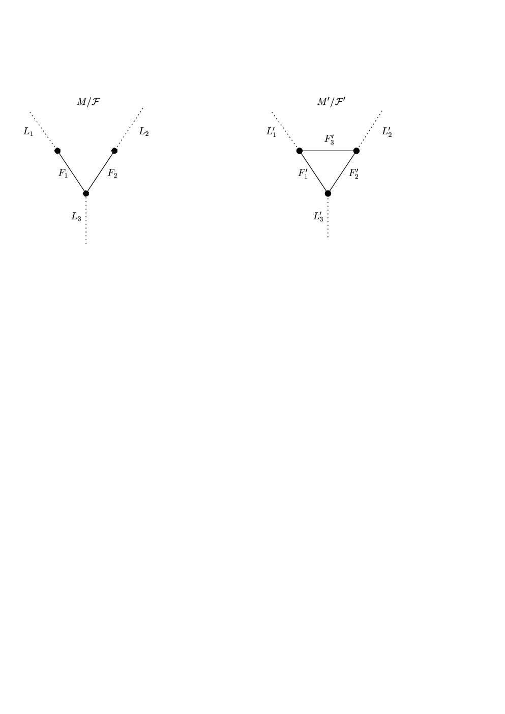
The growth of ff, if it exists, will later be denoted by an orientation of the edges of the macrograph. The micrograph in a vertex of the macrograph regulates the “traffic”, i.e., tells us along which ways in M/ℱM/{\cal F} the function ff is increasing. Therefore the macroedges beginning or ending in some macrovertex are identified with the vertices in the micrograph. The microedges are the irregular points of M/ℱM/{\cal F} and connect the two macroedges from which they are accessible.
For example, the foliations in Figure 3 have in the macrovertices, displayed as bullets in Figure 3(b) and (d), the micrographs as in Figure 4.
      Refer to caption

Figure 4: Corresponding micrographs to the examples above

The system consisting of the macrograph Γ\Gamma and the micrographs γσ\gamma_{\sigma} in the vertices σ∈Γ\sigma\in\Gamma, integrated in Γ\Gamma, is called the graphical configuration of M/ℱM/{\cal F} and is decisive for the global existence of Euler’s multiplier.
It will turn out that two criteria, one on the micrographs and one on the macrograph, are necessary and, together with some topological conditions on the leaves of ℱ{\cal F}, also sufficient for the global existence of Euler’s multiplier.
In a first step, supposing only the first criterion, we will prove the semiglobal existence, i.e., if all micrographs admit the globalization of ff, then for each p∈Mp\in M there is a neighbourhood U~⊂M\tilde{U}\subset M of FpF_{p} and, should the occasion arise, all other leaves belonging to the same macrovertex as FpF_{p} (see Def. 4.3(a), Def. 5.3), saturated with respect to ℱ{\cal F}, such that in U~\tilde{U} Euler’s multiplier can be defined. In this case, if the orientation of one macroedge is chosen, the micrographs of the macrovertices connected to this macroedge determine the orientation of the neighbouring macroedges.
If this condition of semiglobal existence is fulfilled, then the orientability of the macrograph with respect to the regulation of the micrographs and the topological properties of the oriented macrograph decide about the global existence.
In particular, if MM is simply connected, the macrograph and the micrographs of ℱ{\cal F} are also simply connected. By the latter property semiglobal existence is guaranteed, but this even implies global existence by the simply connectedness of the macrograph.
Refer to caption
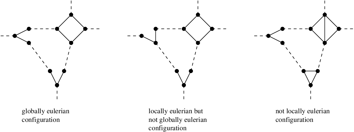
Figure 5: Examples of locally or globally eulerian configurations

In Figure 5 the graphs of three foliations corresponding to the same macrographs are shown. The edges of the macrograph are represented by dotted lines, the edges of the micrographs of the macrovertices by full lines. The terms locally eulerian and globally eulerian are defined in 5.13.
The ideas mentioned above shall be stated more precisely in the following.

5.1 Construction of the graph of a foliation

Having discussed foliations of a certain type in the previous chapter, we want to go into greater detail here and therefore give them a name.

Definition 5.1

Let MM be a real CrC^{r}-manifold of dimension nn++11, ℱ{\cal F} a codim-1-foliation of class CrC^{r} on MM. The foliation ℱ{\cal F} is called graphical if and only if it is of finite type and regularly CrC^{r}.

If a Jordan Brouwer separation theorem holds on MM, we can show that the two conditions in the definition of finite type foliations are not independent. This is done in §​6\lx@sectionsign 6.
Note that the finiteness of p−1​(g)p^{-1}(g) for each g∈Gg\in G implies that GG is Hausdorff.
In what follows, we assume ℱ{\cal F} to be a graphical foliation on a real manifold MM according to Definition 5.1.

Definition 5.2

(Endpoints) Let e∈M/ℱe\in M/{\cal F}. We say that ee is an endpoint if and only if there exists some a∈M/ℱa\in M/{\cal F} such that for each continuous injective mapping w:[0,1]→M/ℱw:[0,1]\to M/{\cal F} with w⁡(0)=aw(0)=a and e∈w⁡([0,1])e\in w([0,1]) holds w⁡(1)=ew(1)=e. Moreover, let EE denote the set of endpoints in M/ℱM/{\cal F}.

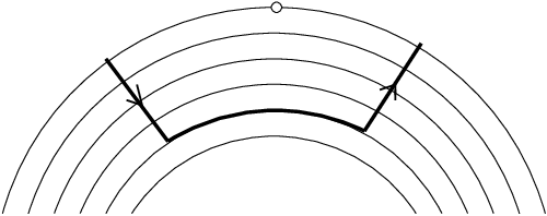
For example, the leaf FF in Figure 6 is such an endpoint.

Refer to caption
Figure 6: Example of an endpoint

Now we are in a position to construct the macrograph of the foliation ℱ{\cal F}.

Construction 5.3

(Macrograph) (a) Vertices: If (S/∼)∪(E/∼)=∅(S/\sim)\cup(E/\sim)=\emptyset take an arbitrary σ∈G\sigma\in G and set 𝒱​Γ0:={σ}{\cal V}\Gamma^{0}:=\{\sigma\}, else let

𝒱Γ0:=(S/∼)∪(E/∼).{\cal V}\Gamma^{0}:=(S/\sim)\cup(E/\sim).

Let us define recursively: (i) If there is a continuous injective mapping w:[0,1)→Gw:[0,1)\to G with w⁡(0)=σ1∈𝒱​Γjw(0)=\sigma_{1}\in{\cal V}\Gamma^{j} and w⁡((0,1))⊂G∖𝒱​Γjw((0,1))\subset G\setminus{\cal V}\Gamma^{j} and the limit limt→1w⁡(t)\displaystyle\lim_{t\to 1}w(t) does not exist, then define

𝒱​Γj+1:=𝒱​Γj∪⋃k∈ℕw⁡(1−1k).{\cal V}\Gamma^{j+1}:={\cal V}\Gamma^{j}\cup\bigcup_{k\in{{\mathbb{N}}}}w\Bigl(1-\frac{1}{k}\Bigr).

(ii) If there is an injective mapping w:[0,1)→Gw:[0,1)\to G with w⁡(0)=σ1∈𝒱​Γjw(0)=\sigma_{1}\in{\cal V}\Gamma^{j} and w⁡((0,1))⊂G∖𝒱​Γjw((0,1))\subset G\setminus{\cal V}\Gamma^{j} and limt→1w⁡(t)=w⁡(0)=σ1\displaystyle\lim_{t\to 1}w(t)=w(0)=\sigma_{1} then define

𝒱​Γj+1:=𝒱​Γj∪w⁡(12).{\cal V}\Gamma^{j+1}:={\cal V}\Gamma^{j}\cup w\Bigl(\frac{1}{2}\Bigr).

As there can only be a countable number of ranges w⁡((,,,))⊂Gw((0,1))\subset G, by choice of a counting it can be obtained that

𝒱​Γ:=⋃j∈ℕ𝒱​Γj{\cal V}\Gamma:=\bigcup_{j\in{{\mathbb{N}}}}{\cal V}\Gamma^{j}

has the property that w⁡(1):=limt→1w⁡(t)w(1):=\lim_{t\to 1}w(t) does exist for every continuous, injective map w:[0,1)→Gw:[0,1)\to G with w⁡(0)=σ1∈𝒱​Γw(0)=\sigma_{1}\in{\cal V}\Gamma and w⁡((,,,))⊂G∖𝒱​Γw((0,1))\subset G\setminus{\cal V}\Gamma, where w⁡(1)≠w⁡(0)w(1)\not=w(0).
Now 𝒱​Γ{\cal V}\Gamma is called the set of vertices of the macrograph Γ\Gamma. Note that S⊂p−1​(𝒱​Γ)S\subset p^{-1}({\cal V}\Gamma), but, in general, there are also noncritical vertices (cf. Remark 5.4).
(b) Edges: To define the edges of the macrograph first we set

𝐖:={w:[0,1]→M/ℱ|w is continuous, ​w|[0,1)​ is injective, w(0),w(1)∈p−1(𝒱Γ),w((0,1))∩p−1(𝒱Γ)=∅}.\begin{split}{\bf W}:=\Big\{w:[0,1]\to M/{\cal F}\ \Big|\ w&\mbox{ is continuous, }w\big|_{[0,1)}\mbox{ is injective, }\\ &w(0),w(1)\in p^{-1}({\cal V}\Gamma),w((0,1))\cap p^{-1}({\cal V}\Gamma)=\emptyset\Big\}.\end{split}

Now we say w∼∗w′w\sim^{*}w^{\prime} for w,w′∈𝐖w,w^{\prime}\in{\bf W} if and only if

p⁡(w⁡([0,1]))​ = ​p​(w′​([0,1]))p\Bigl(w\bigl([0,1]\bigr)\Bigr)\mbox{\hskip 2.84526pt}=\mbox{\hskip 2.84526pt}p\Bigl(w^{\prime}\bigl([0,1]\bigr)\Bigr)

For each L∈𝐖/∼∗L\in{\bf W}/\sim^{*} set an edge LL connecting the corresponding points p⁡(w⁡(0))p(w(0)) and p⁡(w⁡(1))p(w(1)) in 𝒱​Γ{\cal V}\Gamma, i.e., let ℰΓ:=𝐖/∼∗{\cal E}\Gamma:={\bf W}/\sim^{*} be the set of edges of Γ\Gamma.
Now we can define the macrograph Γ=(𝒱​Γ,ℰ​Γ)\Gamma=({\cal V}\Gamma,{\cal E}\Gamma) with the corresponding mapping

(4) κ:ℰΓ→S2𝒱Γ,L↦{p(w(0)),p(w(1))},  where [w]∼∗=L.\kappa:\ {\cal E}\Gamma\to{\it S}^{2}{\cal V}\Gamma,\ L\mapsto\{p(w(0)),p(w(1))\},\quad\mbox{\hskip 2.84526pt}\mbox{ where }\ [w]_{\sim^{*}}=L.

For x∈Mx\in M and L∈ℰ​ΓL\in{\cal E}\Gamma we will write

(5) x∈L :⇔ ∃w∈𝐖:[w]∼∗=L,π(x)∈w((0,1)).x\in L\mbox{\hskip 2.84526pt}:\Leftrightarrow\mbox{\hskip 2.84526pt}\exists w\in{\bf W}:[w]_{\sim^{*}}=L,\ \pi(x)\in w((0,1)).
Remark 5.4

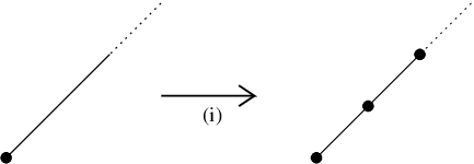
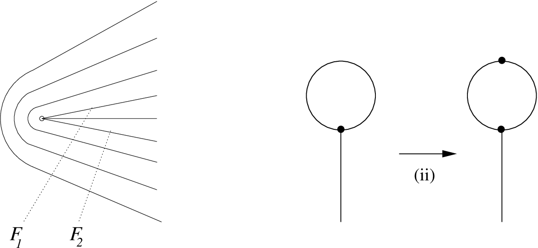
The construction in 5.3 (a) guarantees that each edge of Γ\Gamma connects two different vertices. This is due to the formal definition of graphs in literature. The addition (i) is necessary to avoid edges running to infinity and is illustrated in Figure 8.
Refer to caption
Figure 7: construction (i) in 5.3
Refer to caption
Figure 8: construction (ii) in 5.3

The addition (ii) suppresses loops in Γ\Gamma by adding a ’noncritical’ vertex. An example of a foliation generating such a loop and the corresponding macrograph is shown in Figure 8. Here, the leaves F1F_{1} and F2F_{2} are non-Hausdorff and generate the first vertex. Note that these ’artificial’ vertices have trivial inner structure and are therefore noncritical, cf. Remark 5.6.

Now we investigate the macrovertices and construct the corresponding micrographs.

Construction 5.5

(Micrograph) Let σ∈𝒱Γ∖(E/∼)\sigma\in{\cal V}\Gamma\setminus(E/\sim), p−1​(σ)={s1,…,sN}⊂M/ℱp^{-1}(\sigma)=\big\{s_{1},...,s_{N}\big\}\subset M/{\cal F}. Let ℰ​Γσ:={L1,…,Lν}{\cal E}\Gamma^{\sigma}:=\{L_{1},...,L_{\nu}\} be the set of macroedges LL with σ∈κ⁡(L)\sigma\in\kappa(L), where κ\kappa is defined in (4).
(a) Vertices: Let

𝒱​γσ:={L1,…,Lν}{\cal V}\gamma_{\sigma}:=\big\{L_{1},...,L_{\nu}\big\}

be the set of vertices of the micrograph γσ\gamma_{\sigma} of the macrovertex σ\sigma.
(b) Edges: We say for s∈p−1​(𝒱​Γ)s\in p^{-1}({\cal V}\Gamma) and L∈ℰ​ΓL\in{\cal E}\Gamma

s∈𝐿𝑖𝑚(L):⟺∃w∈𝐖:[w]∼∗=L,w(1)=s.s\in{\it Lim}\ (L)\ :\Longleftrightarrow\ \exists w\in{\bf W}:\ [w]_{\sim^{*}}=L,w(1)=s.

Now we will show that for each leaf sj∈p−1​(σ)s_{j}\in p^{-1}(\sigma) there are exactly two different macroedges LL with sj∈𝐿𝑖𝑚⁡(L)s_{j}\in{\it Lim}(L):
Since s=sj∈p−1​(σ)s=s_{j}\in p^{-1}(\sigma) is no endpoint, there is a continuous bijective mapping w:[0,1]→M/ℱw:[0,1]\to M/{\cal F} with s∈w⁡((,,,))s\in w((0,1)). Let τ∈(0,1)\tau\in(0,1) with w⁡(τ)=sw(\tau)=s. Extending and rescaling w|[0,τ]w|_{[0,\tau]} and w|[τ,1]w|_{[\tau,1]} in an appropriate way we can obtain two different macroedges [w1]∼∗[w_{1}]_{\sim^{*}} and [w2]∼∗[w_{2}]_{\sim^{*}} with s∈𝐿𝑖𝑚([w1]∼∗)∩𝐿𝑖𝑚([w2]∼∗)s\in{\it Lim}([w_{1}]_{\sim^{*}})\cap{\it Lim}([w_{2}]_{\sim^{*}}). Thus there are at least two macroedges connected to ss. Now let x∈s⊂Mx\in s\subset M be any fixed point and (U,φ)(U,\varphi) a foliation chart of (M,ℱ)(M,{\cal F}), where x∈Ux\in U, D⊂ℝnD\subset{\mathbb{R}}^{n}, I=(−ϵ,+ϵ)I=(-\epsilon,+\epsilon) and φ=(φ1,φ2):U→D×I\varphi=(\varphi_{1},\varphi_{2}):U\to D\times I is a bijective CrC^{r} mapping. Now consider the commutative diagram

    M⊃   U    π          φ         D×I    p​r         M/ℱ⊃   V    iV         I    ,\lx@xy@svg{\hbox{\raise 2.5pt\hbox{\kern 6.29515pt\hbox{\ignorespaces\ignorespaces\ignorespaces\hbox{\vtop{\halign{\entry@#!@&&\entry@@#!@\cr&&\cr&&\crcr}}}\ignorespaces{\hbox{\kern-3.0pt\raise 0.0pt\hbox{\hbox{\kern 0.0pt\raise 0.0pt\hbox{\hbox{\kern 9.54858pt\raise-2.5pt\hbox{$\textstyle{M\supset\mbox{\hskip-34.44434pt}}$}}}}}}}{\hbox{\kern 30.3639pt\raise 0.0pt\hbox{\hbox{\kern 0.0pt\raise 0.0pt\hbox{\hbox{\kern 3.0pt\raise-2.5pt\hbox{$\textstyle{U\ignorespaces\ignorespaces\ignorespaces\ignorespaces\ignorespaces\ignorespaces\ignorespaces\ignorespaces}$}}}}}}}\ignorespaces\ignorespaces\ignorespaces\ignorespaces{}{\hbox{\lx@xy@droprule}}\ignorespaces\ignorespaces\ignorespaces{\hbox{\kern 37.32292pt\raise-15.83333pt\hbox{{}\hbox{\kern 0.0pt\raise 0.0pt\hbox{\hbox{\kern 3.0pt\hbox{\hbox{\kern 0.0pt\raise-1.50694pt\hbox{$\scriptstyle{\pi}$}}}\kern 3.0pt}}}}}}\ignorespaces{\hbox{\kern 37.32292pt\raise-24.33334pt\hbox{\hbox{\kern 0.0pt\raise 0.0pt\hbox{\lx@xy@tip{1}\lx@xy@tip{-1}}}}}}{\hbox{\lx@xy@droprule}}{\hbox{\lx@xy@droprule}}\ignorespaces\ignorespaces\ignorespaces\ignorespaces{}{\hbox{\lx@xy@droprule}}\ignorespaces\ignorespaces\ignorespaces{\hbox{\kern 55.19684pt\raise 5.1875pt\hbox{{}\hbox{\kern 0.0pt\raise 0.0pt\hbox{\hbox{\kern 3.0pt\hbox{\hbox{\kern 0.0pt\raise-0.8264pt\hbox{$\scriptstyle{\varphi}$}}}\kern 3.0pt}}}}}}\ignorespaces{\hbox{\kern 68.3507pt\raise 0.0pt\hbox{\hbox{\kern 0.0pt\raise 0.0pt\hbox{\lx@xy@tip{1}\lx@xy@tip{-1}}}}}}{\hbox{\lx@xy@droprule}}{\hbox{\lx@xy@droprule}}{\hbox{\kern 68.3507pt\raise 0.0pt\hbox{\hbox{\kern 0.0pt\raise 0.0pt\hbox{\hbox{\kern 3.0pt\raise-2.5pt\hbox{$\textstyle{D\times I\ignorespaces\ignorespaces\ignorespaces\ignorespaces}$}}}}}}}\ignorespaces\ignorespaces\ignorespaces\ignorespaces{}{\hbox{\lx@xy@droprule}}\ignorespaces\ignorespaces\ignorespaces{\hbox{\kern 84.3305pt\raise-15.83333pt\hbox{{}\hbox{\kern 0.0pt\raise 0.0pt\hbox{\hbox{\kern 3.0pt\hbox{\hbox{\kern 0.0pt\raise-0.8264pt\hbox{$\scriptstyle{pr}$}}}\kern 3.0pt}}}}}}\ignorespaces{\hbox{\kern 84.3305pt\raise-24.33334pt\hbox{\hbox{\kern 0.0pt\raise 0.0pt\hbox{\lx@xy@tip{1}\lx@xy@tip{-1}}}}}}{\hbox{\lx@xy@droprule}}{\hbox{\lx@xy@droprule}}{\hbox{\kern-6.29515pt\raise-31.66666pt\hbox{\hbox{\kern 0.0pt\raise 0.0pt\hbox{\hbox{\kern 3.0pt\raise-2.5pt\hbox{$\textstyle{M/{\cal F}\supset\mbox{\hskip-25.83325pt}}$}}}}}}}{\hbox{\kern 30.29515pt\raise-31.66666pt\hbox{\hbox{\kern 0.0pt\raise 0.0pt\hbox{\hbox{\kern 3.0pt\raise-2.5pt\hbox{$\textstyle{V\ignorespaces\ignorespaces\ignorespaces\ignorespaces}$}}}}}}}\ignorespaces\ignorespaces\ignorespaces\ignorespaces{}{\hbox{\lx@xy@droprule}}\ignorespaces\ignorespaces\ignorespaces{\hbox{\kern 53.39813pt\raise-25.84792pt\hbox{{}\hbox{\kern 0.0pt\raise 0.0pt\hbox{\hbox{\kern 3.0pt\hbox{\hbox{\kern 0.0pt\raise-1.81319pt\hbox{$\scriptstyle{i_{V}}$}}}\kern 3.0pt}}}}}}\ignorespaces{\hbox{\kern 78.74023pt\raise-31.66666pt\hbox{\hbox{\kern 0.0pt\raise 0.0pt\hbox{\lx@xy@tip{1}\lx@xy@tip{-1}}}}}}{\hbox{\lx@xy@droprule}}{\hbox{\lx@xy@droprule}}{\hbox{\kern 78.74023pt\raise-31.66666pt\hbox{\hbox{\kern 0.0pt\raise 0.0pt\hbox{\hbox{\kern 3.0pt\raise-2.5pt\hbox{$\textstyle{I}$}}}}}}}\ignorespaces}}}}\ignorespaces,

where V=π⁡(U)V=\pi(U) and iVi_{V} is, by definition of the local manifold structure of M/ℱM/{\cal F}, a diffeomorphism. Without restriction we can assume φ2​(x)=0\varphi_{2}(x)=0 and therefore we have

iV(wj((0,1))∩V)=(−ϵ,0)  or  iV(wj((0,1))∩V)=(0,+ϵ), j=1,2,i_{V}(w_{j}((0,1))\cap V)=(-\epsilon,0)\mbox{\hskip 2.84526pt}\mbox{ or }\mbox{\hskip 2.84526pt}i_{V}(w_{j}((0,1))\cap V)=(0,+\epsilon),\quad\mbox{\hskip 2.84526pt}j=1,2,

if ϵ>0\epsilon>0 is sufficiently small. But iV​(w1​((0,1))∩V)=iV​(w2​((0,1))∩V)i_{V}(w_{1}((0,1))\cap V)=i_{V}(w_{2}((0,1))\cap V) implies already [w1]∼∗=[w2]∼∗[w_{1}]_{\sim^{*}}=[w_{2}]_{\sim^{*}}. Thus, there are exactly two macroedges LL satisfying s∈𝐿𝑖𝑚⁡(L)s\in{\it Lim}(L).
Now we set ℰ​γσ:={s1,…,sN}{\cal E}\gamma_{\sigma}:=\{s_{1},...,s_{N}\}. For j=1,…,Nj=1,...,N and s∈𝐿𝑖𝑚⁡(Lj1)∩𝐿𝑖𝑚⁡(Lj2)s\in{\it Lim}(L_{j_{1}})\cap{\it Lim}(L_{j_{2}}), where Lj1≠Lj2L_{j_{1}}\not=L_{j_{2}} set the microedge ss connecting the microvertices Lj1L_{j_{1}} and Lj2L_{j_{2}}. Now the micrograph γσ\gamma_{\sigma} is given by γσ=(ℰ​γσ,𝒱​γσ)\gamma_{\sigma}=({\cal E}\gamma_{\sigma},{\cal V}\gamma_{\sigma}) with the corresponding mapping

(6) κσ:ℰ​γσ→S2​𝒱​γσ,sj↦{Lj1,Lj2}.\kappa_{\sigma}:\quad{\cal E}\gamma_{\sigma}\to{\it S}^{2}{\cal V}\gamma_{\sigma},\quad s_{j}\mapsto\{L_{j_{1}},L_{j_{2}}\}.
Remark 5.6

Examples of micrographs are shown in Figure 4. The micrograph of a noncritical macrovertex has trivial structure which is displayed in Figure 9.

Refer to caption
Figure 9: A micrograph of a noncritical macrovertex
Definition 5.7

(Graphical configuration) Let ℱ{\cal F} be a graphical foliation on a real manifold MM according to Definition 5.1, Γ\Gamma the macrograph of M/ℱM/{\cal F} and γσ\gamma_{\sigma} the micrographs of the macrovertices σ∈𝒱​Γ\sigma\in{\cal V}\Gamma according to Constructions 5.3, 5.5. Then δ⁡(F):=(Γ,(γσ)σ)\delta(F):=\bigl(\Gamma,(\gamma_{\sigma})_{\sigma}\bigr) is called the graphical configuration of ℱ{\cal F}.

The following is just a refinement of [CN, Ch. 4, Lemma 5].

Lemma 5.8

Let ℱ{\cal F} be a foliation with only closed leaves on the manifold MM. Then for every leaf FF of ℱ{\cal F} the holonomy is Hol​(F)∈{1,ℤ2}\mbox{\rm Hol}(F)\in\{1,{\mathbb{Z}}_{2}\}. Furthermore, if ℱ{\cal F} is graphical and Hol​(F)=ℤ2\mbox{\rm Hol}(F)={\mathbb{Z}}_{2} then F∈EF\in E, i.e. FF is an endpoint of δ⁡(ℱ)\delta({\cal F}), where δ⁡(ℱ)=(Γ,(γσ)σ)\delta({\cal F})=(\Gamma,(\gamma_{\sigma})_{\sigma}) is the graphical configuration of the foliation ℱ{\cal F}.

The following notion of oriented and bipartite graphs will turn out to be appropriate for the criteria of existence of Euler’s multiplier.

Definition 5.9

(Orientation) Let 𝒢{\cal G} be the macrograph Γ\Gamma (or any other graph). Then a mapping

↑:  ​ℰ𝒢→𝒱𝒢×𝒱𝒢\uparrow\ :\mbox{\hskip 2.84526pt}\mbox{\hskip 2.84526pt}{\cal E}{\cal G}\to{\cal V}{\cal G}\times{\cal V}{\cal G}

is called orientation of 𝒢{\cal G} if and only if  f∘↑=κ,\mbox{\hskip 2.84526pt}\ {\rm f}\ \circ\uparrow\ =\kappa,\ where

f: ​𝒱𝒢×𝒱𝒢→S2​𝒱𝒢, ​(σ1,σ2)↦{σ1,σ2}.{\rm f}:\mbox{\hskip 2.84526pt}{\cal V}{\cal G}\times{\cal V}{\cal G}\to S^{2}{{\cal V}{\cal G}},\mbox{\hskip 2.84526pt}(\sigma_{1},\sigma_{2})\mapsto\{\sigma_{1},\sigma_{2}\}.
Definition 5.10

(bipartite Graph) Let 𝒢=(𝒱𝒢,ℰ𝒢){\cal G}=\bigl({\cal VG},{\cal EG}\bigr) be a micrograph γσ\gamma_{\sigma} or any other graph with corresponding mapping κ\kappa (cf. (6)). The graph 𝒢{\cal G} is called bipartite if and only if there exist two subsets 𝒱+​𝒢{\cal V}_{+}{\cal G}, 𝒱−​𝒢⊂𝒱𝒢{\cal V}_{-}{\cal G}\subset{\cal VG} with the following properties

  1. (a)

    𝒱𝒢=𝒱+​𝒢∪𝒱−​𝒢{\cal VG}={\cal V}_{+}{\cal G}\cup{\cal V}_{-}{\cal G}, 𝒱+​𝒢∩𝒱−​𝒢=∅{\cal V}_{+}{\cal G}\cap{\cal V}_{-}{\cal G}=\emptyset,

  2. (b)

    ∀s∈ℰ𝒢∃L+∈𝒱+​𝒢,L−∈𝒱−​𝒢:κ⁡(s)={L+,L−}\forall s\in{\cal EG}\ \ \exists\ L^{+}\in{\cal V}_{+}{\cal G},\ L^{-}\in{\cal V}_{-}{\cal G}:\ \ \kappa(s)=\{L^{+},L^{-}\}.

The second condition means that only vertices of different classes are connected by edges of 𝒢{\cal G}.

The micrographs of the first and the second example in Fig. 5 are bipartite, whereas two of the micrographs in the right example of Fig. 5 are not bipartite.

5.2 The foliation of a graphical configuration

We want to revert the construction of the graphical configuration. For this purpose we generalize Definition 5.7:

Definition 5.11

A graphical configuration is a tuple (Γ,(γσ)σ)\left(\Gamma,(\gamma_{\sigma})_{\sigma}\right) with a graph Γ\Gamma, graphs γσ\gamma_{\sigma} for every σ∈𝒱​Γ\sigma\in{\cal V}\Gamma such that ℰ​Γσ=𝒱​γσ{\cal E}\Gamma^{\sigma}={\cal V}\gamma_{\sigma}.

For the definition of ℰ​Γσ{\cal E}\Gamma^{\sigma} see Construction 5.5.

Now we can prove

Theorem 5.12

Let δ=(Γ,(γσ)σ)\delta=\left(\Gamma,(\gamma_{\sigma})_{\sigma}\right) be a graphical configuration without endpoints. Then there is closed one-form ω≠0\omega\not=0 on a surface MM (maybe with zeroes), such that the zero locus of ω\omega is smooth and has no zero-dimensional components, the leaves of the so defined foliation ℱ⁡(ω){\cal F}\left(\omega\right) are diffeomorphic to ℝ{{\mathbb{R}}} and δ=δ⁡(ℱ⁡(ω))\delta=\delta\left({\cal F}\left(\omega\right)\right).

Proof:  Let (Γ,↑)\left(\Gamma,\uparrow\right) be an orientation of Γ\Gamma, that means

ℰ​Γ⟶↑𝒱​Γ×𝒱​Γ⟶fS2​𝒱​Γ,{\cal E}\Gamma\stackrel{{\scriptstyle\uparrow}}{{\longrightarrow}}{\cal V}\Gamma\times{\cal V}\Gamma\stackrel{{\scriptstyle{\rm f}}}{{\longrightarrow}}S^{2}{\cal V}\Gamma,

where f is the forgetful map (forgetting the order) and f∘↑=κ{\rm f}\circ\uparrow=\kappa, cf. Definition 5.9. Let us denote an element m∈𝒱​Γ×𝒱​Γm\in{\cal V}\Gamma\times{\cal V}\Gamma by (m1,m2)\left(m_{1},m_{2}\right), and construct as follows. Let for σ∈𝒱​Γ,L∈ℰ​Γ\sigma\in{\cal V}\Gamma,L\in{\cal E}\Gamma denote

L​i​mσ​(L):={s∈ℰ​γσ|L∈κσ​(s)},Lim^{\sigma}\left(L\right):=\left\{s\in{\cal E}\gamma_{\sigma}|L\in\kappa_{\sigma}\left(s\right)\right\},

where κσ\kappa_{\sigma} denotes the boundary map of γσ\gamma_{\sigma} (cf. (6)). For every L∈ℰ​ΓL\in{\cal E}\Gamma define

IL:=[0,1]×(0,1)∖({0}×{ik|i=1,…,k−1}∪{1}×{il|i=1,…,l−1}),I_{L}:=[0,1]\times\left(0,1\right)\setminus\left(\left\{0\right\}\times\left\{\left.\tfrac{i}{k}\right|i=1,...,k-1\right\}\cup\left\{1\right\}\times\left\{\left.\tfrac{i}{l}\right|\ i=1,...,l-1\right\}\right),

if Lim↑1(L)L={s11(L),…,s1​k(L)}Lim^{\uparrow_{1}\left(L\right)}L=\left\{s_{11}\left(L\right),...,s_{1k}\left(L\right)\right\} and Lim↑2(L)L={s21(L),…,s2​l(L)}Lim^{\uparrow_{2}\left(L\right)}L=\left\{s_{21}\left(L\right),...,s_{2l}\left(L\right)\right\}. This means, the sa​b​(L)s_{ab}(L) are the limit points of LL, where a=1,2a=1,2 stands for the two boundary vertices of LL, ordered according to the chosen orientation.

Now take

M=⋃LIL/∼′,M=\bigcup_{L}I_{L}/\sim^{\prime},

where ∼′\sim^{\prime} is defined as follows: If s∈Lim↑i(L)L∩Lim↑j(L′)L′s\in Lim^{\uparrow_{i}\left(L\right)}L\cap Lim^{\uparrow_{j}\left(L^{\prime}\right)}L^{\prime} for one (and then a unique) choice i,j∈{1,2}i,j\in\left\{1,2\right\} and s=si​a​(L)=sj​b​(L′)s=s_{ia}\left(L\right)=s_{jb}\left(L^{\prime}\right) then

IL∋(i−1,a−xk)∼′(j−1,b−xl)∈IL′I_{L}\ni\left(i-1,\frac{a-x}{k}\right)\sim^{\prime}\left(j-1,\frac{b-x}{l}\right)\in I_{L^{\prime}}

for x∈(0,1)x\in\left(0,1\right). This means, that the intervals in ILI_{L} resp IL′I_{L}^{\prime} corresponding to ss are identified.

The so defined topological space MM can easily be made to a differentiable manifold, because after the choice of σ\sigma, the edges {L,L′}=κσ​(s)\left\{L,L^{\prime}\right\}=\kappa_{\sigma}\left(s\right) are unique and therefore a small neighbourhood of every point of MM is topologically an open set in ℝ2{{\mathbb{R}}}^{2}. The differentiability of the transition maps is just a formal calculation. The foliation ℱ{\cal F} is given by x=c​o​n​s​tx=const if (x,y)∈IL\left(x,y\right)\in I_{L}. Since the coordinates of the ILI_{L} can differ at most in the sign, there is a global one-form ω\omega, which is closed and can locally be written

ω=sin⁡(2​π​x)​d​x.\omega=\sin(2\pi x)\ dx\hskip-8.61108pt.

Hence, ω\omega defines the foliation ℱ{\cal F} even in the zero locus of ω\omega. □\square


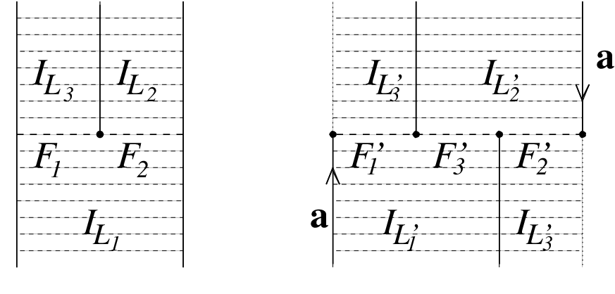
In Fig. 10 we illustrated the rather technical construction of Theorem 5.12 for the graphical configurations of Fig. 4 resp. Fig. 3. In the second case, the right and left boundaries “a{\rm a}” are to be identified in converse direction. Hence the resulting manifold equals a Möbius surface without three certain rays. By a look at the manifold in Fig. 3(c) we see in particular, that the correspondence of graphical configurations and the pairs (M,ℱ)(M,{\cal F}) is not reversible.

Refer to caption
Figure 10:

5.3 The existence of Euler’s multiplier

Now we arrive at the main result of this paragraph which is an equivalent criterion on the graphical configuration δ⁡(ℱ)\delta({\cal F}) for the local or the global existence, respectively, of Euler’s multiplier.

Definition 5.13

(Eulerian configuration) Let ℱ{\cal F} be a graphical CrC^{r} codim-1-foliation on MM, δ⁡(ℱ)=(Γ,(γσ)σ)\delta({\cal F})=\bigl(\Gamma,(\gamma_{\sigma})_{\sigma}\bigr) the graphical configuration of ℱ{\cal F} with respect to the construction in 5.3, 5.5.

  1. (a)

    The configuration δ⁡(ℱ)\delta({\cal F}) is called locally eulerian if and only if E=∅E=\emptyset and for each σ∈𝒱​Γ\sigma\in{\cal V}\Gamma the corresponding micrograph γσ\gamma_{\sigma} is bipartite (cf. Definitions 5.2, 5.10).

  2. (b)

    The configuration δ⁡(ℱ)\delta({\cal F}) is called globally eulerian if and only if the following three conditions hold:

    1. (i)

      δ⁡(ℱ)\delta({\cal F}) is locally eulerian.

    2. (ii)

      The bipartitions 𝒱​γσ​ = ​𝒱+​γσ∪𝒱−​γσ{\cal V}\gamma_{\sigma}\mbox{\hskip 2.84526pt}=\mbox{\hskip 2.84526pt}{\cal V}_{+}\gamma_{\sigma}\cup{\cal V}_{-}\gamma_{\sigma} of σ∈𝒱​Γ\sigma\in{\cal V}\Gamma can be chosen such that, using the notation of 5.5 and 5.10, for σ,σ′∈𝒱​Γ\sigma,\sigma^{\prime}\in{\cal V}\Gamma

      ℰ​Γσ∩ℰ​Γσ′​ = ​(𝒱+​γσ∩𝒱−​γσ′)∪(𝒱−​γσ∩𝒱+​γσ′).{\cal E}\Gamma^{\sigma}\cap{\cal E}\Gamma^{\sigma^{\prime}}\mbox{\hskip 2.84526pt}=\mbox{\hskip 2.84526pt}\bigl({\cal V}_{+}\gamma_{\sigma}\cap{\cal V}_{-}\gamma_{\sigma^{\prime}}\bigr)\cup\bigl({\cal V}_{-}\gamma_{\sigma}\cap{\cal V}_{+}\gamma_{\sigma^{\prime}}\bigr).
    3. (iii)

      There are no cycles σ1​L1​σ2​L2​σ3​…​σN​LN​σ1\sigma_{1}L_{1}\sigma_{2}L_{2}\sigma_{3}...\sigma_{N}L_{N}\sigma_{1} with Li∈𝒱+​γσiL_{i}\in{\cal V}_{+}\gamma_{\sigma_{i}} for all i=1,…,Ni=1,...,N or Li∈𝒱−​γσiL_{i}\in{\cal V}_{-}\gamma_{\sigma_{i}} for all i=1,…,Ni=1,...,N, where N∈ℕN\in{\mathbb{N}}.

At this occasion, we want to point out that Definition 5.13 has nothing to do with the usual definition of an eulerian graph in literature.

Remark 5.14

Obviously, the definition of a global eulerian configuration in Definition 5.13 (b) is equivalent to the following:
The configuration δ⁡(ℱ)\delta({\cal F}) is globally eulerian if and only if there is an orientation

↑:ℰΓ→𝒱Γ×𝒱Γ,L↦(↑1(L),↑2(L))\uparrow\ :{\cal E}\Gamma\to{\cal V}\Gamma\times{\cal V}\Gamma,\ L\mapsto\bigl(\uparrow_{1}(L),\uparrow_{2}(L)\bigr)

of Γ\Gamma (cf. Def. 5.9) such that the following three conditions hold:

    1. (i)

      E=∅E=\emptyset.

    2. (ii)

      For each σ∈𝒱​Γ\sigma\in{\cal V}\Gamma the micrograph γσ\gamma_{\sigma} is bipartite such that, using the notation of Definition 5.10,

      𝒱+γσ={L∈𝒱γσ|↑1(L)=σ},𝒱−γσ={L∈𝒱γσ|↑2(L)=σ}.{\cal V}_{+}{\gamma_{\sigma}}=\big\{L\in{\cal V}\gamma_{\sigma}\big|\uparrow_{1}(L)=\sigma\big\},\quad{\cal V}_{-}{\gamma_{\sigma}}=\big\{L\in{\cal V}\gamma_{\sigma}\big|\uparrow_{2}(L)=\sigma\big\}.
    3. (iii)

      The orientation ↑\uparrow induces a well-defined partial ordering “≤\leq” on 𝒱​Γ{\cal V}\Gamma by

      σ<σ′:⟺∃N∈ℕ,τ1,…,τN∈𝒱​Γ,L1,…,LN−1∈ℰ​Γ:τ1=σ,τN=σ′,↑(Lj)=(τj,τj+1), j=1,…,N−1,\begin{split}\sigma<\sigma^{\prime}\ :\Longleftrightarrow\ &\exists N\in{\mathbb{N}},\ \tau_{1},...,\tau_{N}\in{\cal V}\Gamma,\ L_{1},...,L_{N-1}\in{\cal E}\Gamma:\\ &\tau_{1}=\sigma,\ \tau_{N}=\sigma^{\prime},\ \uparrow(L_{j})=(\tau_{j},\tau_{j+1}),\mbox{ \footnotesize$j=1,...,N$$-$$1$},\end{split}

      where σ<σ′\sigma<\sigma^{\prime} means σ≤σ′\sigma\leq\sigma^{\prime} but σ≠σ′\sigma\not=\sigma^{\prime}.

Examples of locally eulerian or globally eulerian configurations are illustrated in Fig. 5.
In order to formulate our criterion for semiglobal existence of Euler’s multiplier, we need some technical preparations:

Definition 5.15

A curve α:[a,b]→M\alpha:[a,b]\to M of class CrC^{r} is called transversal, if the mapping π∘α:[a,b]→M/ℱ\pi\circ\alpha:[a,b]\to M/{\cal F} is injective and

∀t∈[a,b]:dd​t​(π∘α)​(t)≠0.\forall t\in[a,b]:\quad\frac{d}{dt}\bigl(\pi\circ\alpha\bigr)(t)\not=0.
Remark 5.16

Let U⊂G=(M/ℱ)/∼U\subset G=(M/{\cal F})/\sim an open set and p:M/ℱ→Gp:M/{\cal F}\to G the canonical projection (cf. Def. 4.3(a)). Then U~:=π−1​(p−1​(U))\tilde{U}:=\pi^{-1}\bigl(p^{-1}(U)\bigr) is a saturated set in MM satisfying

F∈ℱ,F∩U~≠∅​  ⇒ ​⋃F′∈[F]∼​F′⊂U~,F\in{\cal F},\ F\cap\tilde{U}\not=\emptyset\mbox{\hskip 2.84526pt}\mbox{\hskip 2.84526pt}\Rightarrow\mbox{\hskip 2.84526pt}\bigcup_{F^{\prime}\in[F]_{\sim}}\mbox{\hskip-8.61108pt}F^{\prime}\ \subset\ \tilde{U},

i.e. if F∩U~≠∅F\cap\tilde{U}\not=\emptyset for any leaf FF then U~\tilde{U} is a common saturated neighbourhood of all leaves F′∈ℱF^{\prime}\in{\cal F} with F′∈[F]∼F^{\prime}\in[F]_{\sim} according to Definition 4.3(a) (b).

Lemma 5.17

Let r≥1r\geq 1 and ℱ{\cal F} be a graphical CrC^{r} codim-1-foliation. Then the following conditions are equivalent:

  1. (a)

    δ⁡(ℱ)\delta({\cal F}) is locally eulerian.

  2. (b)

    For each xx∈\inMM there is some neighbourhood UU⊂\subsetGG of p⁡(π⁡(x))p\bigl(\pi(x)\bigr), such that there is ff∈\inCr​(U~,ℝ)C^{r}\bigl(\tilde{U},{\mathbb{R}}\bigr) with d​f​(x)≠0df(x)\not=0 in U~\tilde{U} and ℱ|U~=ℱ⁡(d​f){\cal F}|_{\tilde{U}}={\cal F}(df), where U~:=π−1​(p−1​(U))\tilde{U}:=\pi^{-1}\bigl(p^{-1}(U)\bigr).

Condition (b) means the semiglobal existence of ff.

Proof:  Let (a) be satisfied. The transverse orientability of ℱ{\cal F} and the existence of a piecewise CrC^{r} function f0f_{0} without extrema like described are rather technical to prove, but plausible. So we omit this part. Furthermore it is clear that after any choice of a non-Hausdorff leaf F0F_{0} the function f0f_{0} can be chosen CrC^{r} around F0F_{0} with d​f0≠0df_{0}\not=0 on F0F_{0}. Now CrC^{r}-regularity and transverse orientability of ℱ{\cal F} imply that there is a saturated neighbourhood U0U_{0} of F0F_{0} and a function f~∈Cℱr​(M)\tilde{f}\in C^{r}_{\cal F}(M) such that f0|U0=f~|U0f_{0}|U_{0}=\tilde{f}|U_{0}. For any Fi∼F0F_{i}\sim F_{0} holds automatically d​f~≠0d\tilde{f}\not=0 on FiF_{i}: Let TT be a local transversal through x∈F0x\in F_{0} with injective projection to M/ℱM/{\cal F}; this exists, since we assumed E=∅E=\emptyset. The function x∈Ft​(t∈T)↦1d​f~​(∂∂t)x\in F_{t}(t\in T)\mapsto\frac{1}{d\tilde{f}(\frac{\partial}{\partial t})} would be in Cℱr−1​(sat​(T))C^{r-1}_{\cal F}(\mbox{sat}(T)) and not be extendable beyond FiF_{i}, if d​f~|Fi=0d\tilde{f}|F_{i}=0. So for all Fi∼FF_{i}\sim F there is a saturated neighbourhood Ui⊃FiU_{i}\supset F_{i} such that d​f~≠0d\tilde{f}\not=0 on UiU_{i}. We set U:=⋃Fi∈[F]UiU:=\bigcup_{F_{i}\in[F]}U_{i} and f:=f~|Uf:=\tilde{f}|U.

In order to prove the other direction, (b)⇒(a){(b)}\Rightarrow{(a)}, the arguments are again technical, but straightforward. □\square

Theorem 5.18

(Criterion for global existence) Let ℱ{\cal F} be a graphical CrC^{r} codim-1-foliation. Then the following conditions are equivalent:

  1. (a)

    δ⁡(ℱ)\delta({\cal F}) is globally eulerian.

  2. (b)

    There is some function f∈Cr​(M,ℝ)f\in C^{r}(M,{\mathbb{R}}) such that d​f​(x)≠0df(x)\not=0 in MM and ℱ=ℱ⁡(d​f){\cal F}={\cal F}(df).

Proof:  (i) Suppose δ⁡(ℱ)\delta({\cal F}) to be globally eulerian. Let ℛ:=𝒱​Γ{\cal R}:={\cal V}\Gamma be partially ordered according to 5.14 ()(iii) and let a:𝒱​Γ→ℚ{\rm a}:{\cal V}\Gamma\to{\mathbb{Q}} be any mapping satisfying

σ<σ′⟹a⁡(σ)<a⁡(σ′)\sigma<\sigma^{\prime}\Longrightarrow{\rm a}(\sigma)<{\rm a}(\sigma^{\prime})

Moreover, for each σ∈𝒱​Γ\sigma\in{\cal V}\Gamma choose ϵσ∈(0,1)\epsilon_{\sigma}\in(0,1) with

(7) ϵσ<13min{|a(σ′)−a(σ)||σ′∈𝒱Γ,∃L∈ℰΓ:κ(L)={σ,σ′}}.\epsilon_{\sigma}<\frac{1}{3}\ {\rm min}\ \Big\{\ |{\rm a}(\sigma^{\prime})-{\rm a}(\sigma)|\ \Big|\ \sigma^{\prime}\in{\cal V}\Gamma,\ \exists L\in{\cal E}\Gamma:\kappa(L)=\{\sigma,\sigma^{\prime}\}\Big\}.

Let U~σ\tilde{U}_{\sigma} be an appropriate neighbourhood of σ\sigma, x∈s∈ℰ​γσx\in s\in{\cal E}\gamma_{\sigma} and fσ∈Cr​(U~σ,ℝ)f_{\sigma}\in C^{r}\bigl(\tilde{U}_{\sigma},{\mathbb{R}}\bigr) the corresponding mapping as in condition (b) of Lemma 5.17. Without any restriction we may assume fσ​(x)∈[−ϵσ,+ϵσ]f_{\sigma}(x)\in[-\epsilon_{\sigma},+\epsilon_{\sigma}] for each x∈U~σx\in\tilde{U}_{\sigma} and U~σ∩U~σ′=∅\tilde{U}_{\sigma}\cap\tilde{U}_{\sigma^{\prime}}=\emptyset for σ′∈𝒱​Γ∖{σ}\sigma^{\prime}\in{\cal V}\Gamma\setminus\{\sigma\}. Now define

f~:⋃σ∈𝒱​ΓU~σ→ℝ,f~​(x):=a⁡(σ)+fσ​(x)​  for  ​x∈U~σ.\tilde{f}:\ \bigcup_{\sigma\in{\cal V}\Gamma}\tilde{U}_{\sigma}\to{\mathbb{R}},\ \tilde{f}(x):={\rm a}(\sigma)+f_{\sigma}(x)\mbox{\hskip 2.84526pt}\mbox{ for }\mbox{\hskip 2.84526pt}x\in\tilde{U}_{\sigma}.

Let L∈ℰ​ΓL\in{\cal E}\Gamma, κ⁡(L)={σ,σ′}\kappa(L)=\{\sigma,\sigma^{\prime}\}, L∈𝒱+​γσ∩𝒱−​γσ′L\in{\cal V}_{+}\gamma_{\sigma}\cap{\cal V}_{-}\gamma_{\sigma^{\prime}}. Thus, we have a⁡(σ)<a⁡(σ′){\rm a}(\sigma)<{\rm a}(\sigma^{\prime}) and, using condition (7),

∀x∈U~σ,x′∈U~σ′:f~​(x)<f~​(x′).\forall x\in\tilde{U}_{\sigma},\ x^{\prime}\in\tilde{U}_{\sigma^{\prime}}:\quad\tilde{f}(x)<\tilde{f}(x^{\prime}).

Moreover, let u∈Cr​([0,1],M)u\in C^{r}\bigl([0,1],M\bigr) be some transversal curve according to 5.15 such that π∘u∈𝐖\pi\circ u\in{\bf W} and L=[π∘u]∼L=[\pi\circ u]_{\sim} (For the definition of 𝐖{\bf W} see Construction 5.3). For x∈Mx\in M with x∈Lx\in L according to (5) we define

f⁡(x):=ϕ⁡((π∘u)−1​(π⁡(x))).f(x):=\phi\Bigl(\bigl(\pi\circ u\bigr)^{-1}\bigl(\pi(x)\bigr)\Bigr).

for a suitably chosen strictly increasing function ϕ∈Cr​([0,1])\phi\in C^{r}([0,1]). After an appropriate reparametrization of uu, we can achieve f​(x)=f~σ​(x)f(x)=\tilde{f}_{\sigma}(x) for x∈U~σx\in\tilde{U}_{\sigma}, σ∈𝒱​Γ\sigma\in{\cal V}\Gamma. Then ff has the desired properties.
(ii) Now suppose condition (b) to be fulfilled. From Lemma 5.17 we know that Γ\Gamma is locally eulerian. An ordering on 𝒱​Γ{\cal V}\Gamma and therefore an orientation ↑\uparrow of Γ\Gamma according to Remark 5.14 (iii) is induced by ff, given by

σ<σ′​ if ​f​(ξ)<f⁡(ξ′),\sigma<\sigma^{\prime}\text{\quad if \quad}f(\xi)<f(\xi^{\prime}),

where σ,σ′∈𝒱​Γ\sigma,\sigma^{\prime}\in{\cal V}\Gamma, ξ,ξ′∈M\xi,\xi^{\prime}\in M with p⁡(π⁡(ξ))=σp\bigl(\pi(\xi)\bigr)=\sigma, p⁡(π⁡(ξ′))=σ′p\bigl(\pi(\xi^{\prime})\bigr)=\sigma^{\prime} (cf. Def. 4.3(a))
Furthermore, to see the bipartition of 𝒱​γσ{\cal V}\gamma_{\sigma}, define 𝒱+​γσ{\cal V}_{+}\gamma_{\sigma}, 𝒱−​γσ{\cal V}_{-}\gamma_{\sigma} as in Remark 5.14 (ii). □\square

5.4 The case b1​(M)=0b_{1}(M)=0

If ℱ{\cal F} is a graphical foliation, then denote δ⁡(ℱ)=(Γ,(γσ)σ)\delta({\cal F})=(\Gamma,(\gamma_{\sigma})_{\sigma}) the graphical configuration. Like above, we denote Γ=(𝒱​Γ,ℰ​Γ)\Gamma=({\cal V}\Gamma,{\cal E}\Gamma) and similar for other graphs. Let us define the main graph μ=μ⁡(ℱ)\mu=\mu({\cal F}) by

𝒱​μ:=⋃σ∈𝒱​Γ𝒱​γσ,ℰ​μ:=ℰ​Γ∪⋃σ∈𝒱​Γℰ​γσ{\cal V}\mu:=\bigcup_{\sigma\in{\cal V}\Gamma}{\cal V}\gamma_{\sigma},\quad{\cal E}\mu:={\cal E}\Gamma\cup\bigcup_{\sigma\in{\cal V}\Gamma}{\cal E}\gamma_{\sigma}

and the corresponding boundary mapping

κμ: ​ℰ​μ→S2​𝒱​μ, ​κμ​(Λ):={κσ​(Λ), if ​Λ∈ℰ​γσ{Λσ,Λσ′}, if ​Λ∈ℰ​Γ,\kappa_{\mu}:\mbox{\hskip 2.84526pt}\ {\cal E}\mu\to S^{2}{\cal V}\mu,\mbox{\hskip 2.84526pt}\ \kappa_{\mu}(\Lambda):=\left\{\begin{array}[]{ll}\kappa_{\sigma}(\Lambda),&\mbox{ if }\Lambda\in{\cal E}\gamma_{\sigma}\\ \{\Lambda_{\sigma},\Lambda_{\sigma^{\prime}}\},&\mbox{ if }\Lambda\in{\cal E}\Gamma\end{array}\right.,

where in the second case {σ,σ′}=κΓ​(Λ)=κ⁡(Λ)\{\sigma,\sigma^{\prime}\}=\kappa_{\Gamma}(\Lambda)=\kappa(\Lambda) (cf. (4) in Construction 5.3) and Λσ\Lambda_{\sigma} denotes Λ\Lambda as element of 𝒱​γσ{\cal V}\gamma_{\sigma}, correspondingly for σ′\sigma^{\prime}.

This means, that μ\mu is the graph we obtain, if we replace the vertices of Γ\Gamma with their corresponding micrographs.

Let μ\mu and Γ\Gamma also denote the topological space associated to the graph μ\mu resp. Γ\Gamma. Then it is clear that there is a continuous map

c:μ⟶Γ,c:\mu\longrightarrow\Gamma,

which contracts the γσ\gamma_{\sigma} to the point σ\sigma and is an isomorphism outside the micrographs. Moreover, there is a continuous map

c~:μ⟶M/ℱ,\tilde{c}:\mu\longrightarrow M/{\cal F},

which identifies the edges of γσ\gamma_{\sigma} with the corresponding non-Hausdorff leaves in M/ℱM/{\cal F}, and is an isomorphism outside the micrographs. This map satisfies c=p∘c~c=p\circ\tilde{c}. The fibres c−1​(g)c^{-1}(g) of c~\tilde{c} are homeomorphic to intervals, hence they are simply connected. Outside of the micrographs c~\tilde{c} is an isomorphism and M/ℱM/{\cal F} is a one-dimensional manifold outside the non-Hausdorff points. As usual, we denote b1​(Y):=r​k​H1​(Y,ℤ)b_{1}(Y):=rkH^{1}(Y,{\mathbb{Z}}) for a topological space YY.

By standard topological methods we obtain H1​(M/ℱ,ℤ)≅H1​(μ,ℤ)H^{1}(M/{\cal F},{\mathbb{Z}})\cong H^{1}(\mu,{\mathbb{Z}}). Applying this we arrive at

Lemma 5.19

If δ⁡(ℱ)\delta({\cal F}) is the graphical configuration of a foliation, then

  1. (a)

    b1​(M/ℱ)≤b1​(M)b_{1}(M/{\cal F})\leq b_{1}(M),

  2. (b)

    b1​(Γ)+∑σ∈𝒱​Γb1​(γσ)=b1​(M/ℱ),b_{1}(\Gamma)+\sum_{\sigma\in{\cal V}\Gamma}b_{1}(\gamma_{\sigma})=b_{1}(M/{\cal F}),

  3. (c)

    Γ\Gamma and all γσ\gamma_{\sigma} are simply connected, if b1​(M/ℱ)=0b_{1}(M/{\cal F})=0.

Now we can derive the global existence theorem for manifolds with b1​(M)=0b_{1}(M)=0:

Theorem 5.20

Let MM be a manifold with b1​(M)=0b_{1}(M)=0 and ℱ{\cal F} a graphical CrC^{r} codim-1-foliation. Then there is a CrC^{r} function f:M⟶ℝf:M\longrightarrow{\mathbb{R}} with d​f​(x)≠0df(x)\not=0 everywhere and ℱ=ℱ⁡(d​f){\cal F}={\cal F}(df).

Proof: By Lemma 5.19 we know, that Γ\Gamma and all γσ\gamma_{\sigma} are simply connected, so they contain no cycle. Since a graph is bipartite if and only if every cycle has an even number of edges, we conclude, that all γσ\gamma_{\sigma} are bipartite, hence δ⁡(ℱ)\delta({\cal F}) is locally eulerian. Now let us define an orientation of Γ\Gamma inductively: choose any σ∈𝒱​Γ\sigma\in{\cal V}\Gamma and a bipartition

𝒱​γσ=𝒱+​γσ∪𝒱−​γσ.{\cal V}\gamma_{\sigma}={\cal V}_{+}\gamma_{\sigma}\cup{\cal V}_{-}\gamma_{\sigma}\hskip-8.61108pt.

For any L∈ℰ​ΓσL\in{\cal E}\Gamma^{\sigma} choose the orientation ↑(L)\uparrow(L) and the bipartition of the neighboured micrographs so that

↑1(L)=σ∧L∈𝒱−γ↑2(L),\displaystyle\uparrow_{1}(L)=\sigma\wedge L\in{\cal V}_{-}\gamma_{\uparrow_{2}(L)}\ , if L∈𝒱+​γσ,\displaystyle L\in{\cal V}_{+}\gamma_{\sigma},
↑2(L)=σ∧L∈𝒱+γ↑1(L),\displaystyle\uparrow_{2}(L)=\sigma\wedge L\in{\cal V}_{+}\gamma_{\uparrow_{1}(L)}\ , if L∈𝒱−​γσ.\displaystyle L\in{\cal V}_{-}\gamma_{\sigma}.

Now we are looking at the neighbouring micrographs and repeat this procedure. This will give a complete system of orientation of Γ\Gamma and bipartitions of the γσ\gamma_{\sigma}, because Γ\Gamma is connected. We have to show that there are no inconsistencies. But if there are any, say at γσ′\gamma_{\sigma^{\prime}}, there would be two different paths

σ​L1​σ1​…​σk−1​Lk​σ′\displaystyle\sigma L_{1}\sigma_{1}...\sigma_{k-1}L_{k}\sigma^{\prime} resp. σ​Lk​σk​…​σl−1​Ll​σ′.\displaystyle\sigma L_{k}\sigma_{k}...\sigma_{l-1}L_{l}\sigma^{\prime}.

Hence the path

σ​L1​σ1​…​σk−1​Lk​σ′​Ll​σl−1​…​σk​Lk​σ\sigma L_{1}\sigma_{1}...\sigma_{k-1}L_{k}\sigma^{\prime}L_{l}\sigma_{l-1}...\sigma_{k}L_{k}\sigma

would contain a circuit, what contradicts b1​(Γ)=0b_{1}(\Gamma)=0.

In particular, there can be no oriented circuits, so we conclude that δ⁡(ℱ)\delta({\cal F}) is globally eulerian. By Theorem 5.18 the proof is finished. □\square

6 Applications

6.1 Tools

This section is intended to provide tools for the investigation of foliations. In particular, there is some simplification for the test of the graphicalness of a foliation.

6.1.1 Closedness of leaves

If we assume a leaf FF of a C∞C^{\infty} codim-1-foliation ℱ{\cal F} on a manifold MM to be not closed (topological), then FF as a point in M/ℱM/{\cal F} is a non-Hausdorff point. This we see by considering F¯\overline{F}. It is easy to see that F¯\overline{F} is saturated, hence there exists a leaf F′⊂F¯∖FF^{\prime}\subset\overline{F}\setminus F. Clearly, F′F^{\prime} and FF cannot be separated by open neighbourhoods. Hence Hausdorff leaves are closed.

If we want to verify the graphicalness of a foliation it turns out that this gets much simpler, if on MM the Jordan Brouwer Separation Theorem holds for closed leaves, that means:

Definition 6.1

A manifold MM is called foliated Jordan Brouwer separable (fJBS), if for any C∞C^{\infty} codim-1-foliation ℱ{\cal F} and closed leaf F∈ℱF\in{\cal F} holds: M∖FM\setminus F has at least two connected components.

Lemma 6.2

Any manifold MM with H1​(M,ℤ)=0H_{1}(M,{\mathbb{Z}})=0 is fJBS.

Proof: For any manifold ZZ we denote by 𝒜Z{\cal A}_{Z} the sheaf of C∞C^{\infty} functions on ZZ. Let FF be a closed leaf of a foliation ℱ{\cal F} and U⁡(F)U(F) a small tubular neighbourhood. The condition H1​(M,ℤ)H_{1}(M,{\mathbb{Z}}) implies that the part of the Mayer-Vietoris sequence

0⟶H0​(U⁡(F)∖F,ℤ)⟶H0​(M∖F,ℤ)⊕H0​(F,ℤ)⟶H0​(M,ℤ)⟶00\longrightarrow H_{0}(U(F)\setminus F,{\mathbb{Z}})\longrightarrow H_{0}(M\setminus F,{\mathbb{Z}})\oplus H_{0}(F,{\mathbb{Z}})\longrightarrow H_{0}(M,{\mathbb{Z}})\longrightarrow 0

is exact. Since H0​(U⁡(F)∖F,ℤ)=H0​(|NF|∖F,ℤ)H_{0}(U(F)\setminus F,{\mathbb{Z}})=H_{0}(|N_{F}|\setminus F,{\mathbb{Z}}), if |NF||N_{F}| denotes the total space of the normal bundle of FF, it is enough to show NF≅𝒜FN_{F}\cong{\cal A}_{F}: Then |NF|=F×ℝ|N_{F}|=F\times{\mathbb{R}}, hence |NF|∖F=F×(ℝ∖{0})|N_{F}|\setminus F=F\times({\mathbb{R}}\setminus\{0\}).

The crucial point is now that NFN_{F} extends to the line bundle NℱN_{\cal F} on MM. Real line bundles are parametrised by H1​(M,ℤ2)H^{1}(M,{\mathbb{Z}}_{2}), however. By the universal coefficient lemma this group vanishes, so any line bundle on MM is trivial, in particular Nℱ≅𝒜MN_{\cal F}\cong{\cal A}_{M}. This again implies NF≅𝒜FN_{F}\cong{\cal A}_{F}.

Note that we even proved that M∖FM\setminus F has exactly two components. □\square

Lemma 6.3

Let MM be fJBS manifold and ℱ{\cal F} a codim-1-foliation on MM. Then the set

C:={F∈M/ℱ|F is a closed leaf}C:=\left\{F\in\left.M/{\cal F}\ \right|\ F\mbox{ is a closed leaf}\right\}

is closed.

The proof is straightforward and hence left to the reader.

Note that a leaf F⊂MF\subset M is closed if and only if F∈M/ℱF\in M/{\cal F} is a closed point.

The lemma implies immediately:

Corollary 6.4

Let MM be a fJBS manifold. Then a regular CrC^{r} codim-1-foliation ℱ{\cal F} is graphical if and only if p⁡(S)p(S) is a discrete set, and for every g∈Gg\in G the fibre p−1​(g)p^{-1}(g) is a finite set, where SS is like in Definition 4.3(a) the set of non-Hausdorff points.

Proof:  By the discreteness assumption, G∖p⁡(S)G\setminus p(S) is open and dense, hence H:=M/ℱ∖SH:=M/{\cal F}\setminus S is open, since pp is continuous, and dense, since the fibres are finite. But HH is the set of Hausdorff points, hence H⊂CH\subset C. This means by Lemma 6.3 that C=C¯=M/ℱC=\overline{C}=M/{\cal F}, hence all leaves are closed. □\square

6.1.2 Characterization of infinitely near leaves

Here we give criteria for constructing the graphical configuration directly from the one-form. We suppose MM to be Riemannian. Then we have the notion of the normal bundle NℱN_{\cal F} to ℱ{\cal F}, defined by

Nℱ,x:=(Tx​Fx)⟂,N_{{\cal F},x}:=(T_{x}F_{x})^{\perp},

where FxF_{x} is the leaf containing xx. A normal curve b:[0,1]⟶Mb:[0,1]\longrightarrow M then is a curve with b˙​(t)∈Nℱ,b⁡(t)\dot{b}(t)\in N_{{\cal F},b(t)} for all t∈[0,1]t\in[0,1], i.e. an integral curve of the normal bundle.


Let us define a normal path β\beta connecting x∈Fx\in F and x′∈F′x^{\prime}\in F^{\prime} as the sum ν+b+ν′\nu+b+\nu^{\prime}, where ν,ν′:I⟶M\nu,\nu^{\prime}:I\longrightarrow M are paths whose image is contained in the curve normal to ℱ{\cal F} meeting xx resp x′x^{\prime} and ν⁡(0)=x,ν′​(1)=x′\nu(0)=x,\nu^{\prime}(1)=x^{\prime}, and bb is a path whose image is contained in a leaf F~\tilde{F} and ν⁡(1)=b⁡(0),b⁡(1)=ν′​(0).\nu(1)=b(0),b(1)=\nu^{\prime}(0)\hskip-8.61108pt.

Refer to caption
Figure 11: A normal path
Lemma 6.5

Let ω\omega be an integrable one-form without zeroes on the Riemannian manifold (M,g)(M,g) and ℱ=ℱ⁡(ω){\cal F}={\cal F}(\omega) the induced foliation. Then the classes of any two leaves FF and F′F^{\prime} are infinitely near in M/ℱM/{\cal F} if and only if for some (and hence all) x∈F,x′∈F′x\in F,x^{\prime}\in F^{\prime} and all ε>0\varepsilon>0 exists a piecewise continuous differentiable normal path β:[0;1]⟶M\beta:[0;1]\longrightarrow M with β⁡(0)=x,β⁡(1)=x′\beta(0)=x,\beta(1)=x^{\prime} and

∫β|ω|:=∫01|β∗​(ω)​(dd​s)|​𝑑s<ε.\int_{\beta}|\omega|:=\int_{0}^{1}|\beta^{*}(\omega)(\frac{d}{ds})|ds<\varepsilon\hskip-8.61108pt.

Proof: ′⇒′{}^{\prime}\Rightarrow^{\prime}: If F,F′F,F^{\prime} are infinitely near, then by definition, any saturated neighbourhoods

Uδ(F):={F~∈M/ℱ|infx∈F,x~∈F~(distg(x,x~))<δ}U_{\delta}(F):=\left\{\tilde{F}\in M/{\cal F}\ \left|\inf_{x\in F,\tilde{x}\in\tilde{F}}(dist_{g}(x,\tilde{x}))\right.<\delta\right\}

and, analogously defined, Uδ​(F′)U_{\delta}(F^{\prime}) satisfy

Uδ​(F)∩Uδ​(F′)≠∅.U_{\delta}(F)\cap U_{\delta}(F^{\prime})\not=\emptyset\hskip-8.61108pt.

So, if Bδ​(x)B_{\delta}(x) is the geodesic ball of radius δ\delta around xx and lx:[0;1]⟶Bδ​(x)l_{x}:[0;1]\longrightarrow B_{\delta}(x) is a curve normal to ℱ{\cal F} with lx​(0)=xl_{x}(0)=x, and analogously for lx′l_{x^{\prime}}, such that there is a leaf F~\tilde{F} with lx​(1)∈F~∋lx′​(1)l_{x}(1)\in\tilde{F}\ni l_{x^{\prime}}(1), then let α:[0;1]⟶F~\alpha:[0;1]\longrightarrow\tilde{F} be a path from lx​(1)l_{x}(1) to lx′​(1)l_{x^{\prime}}(1) and finally

β:=lx+α+lx′.\beta:=l_{x}+\alpha+l_{x^{\prime}}\hskip-8.61108pt.

Clearly, β\beta is a normal path. If we choose δ\delta sufficiently small, we can achieve

(8) ∫β|ω|<ε.\int_{\beta}|\omega|<\varepsilon.

′⇐′{}^{\prime}\Leftarrow^{\prime}: Let UU and U′U^{\prime} be small saturated neighbourhoods of FF resp. F′F^{\prime}. It is an easy argument, that for sufficiently small ε>0\varepsilon>0, the normal paths βε\beta_{\varepsilon} are contained in U∩U′U\cap U^{\prime}. In particular, U∩U′≠∅U\cap U^{\prime}\not=\emptyset.

□\square

Lemma 6.6

Let ω\omega be an integrable one-form without zeroes on the complete Riemannian manifold MM and ℱ=ℱ⁡(ω){\cal F}={\cal F}(\omega) the induced foliation. FF and F′F^{\prime} are infinitely near in M/ℱM/{\cal F} if and only if for any saturated neighbourhoods U⁡(F),U′​(F′)U(F),U^{\prime}(F^{\prime}) there is a by arc length parametrized curve ν:ℝ+⟶M\nu:{\mathbb{R}}^{+}\longrightarrow M which is normal to the foliation, with ν⁡(ℝ+)∩F=∅,\nu({\mathbb{R}}^{+})\cap F=\emptyset, ν⁡(ℝ+)∩F′=∅\nu({\mathbb{R}}^{+})\cap F^{\prime}=\emptyset, but ν⁡(ℝ+)∩U⁡(F)∩U′​(F′)≠∅\nu({\mathbb{R}}^{+})\cap U(F)\cap U^{\prime}(F^{\prime})\not=\emptyset.

Proof: ′⇐′{}^{\prime}\Leftarrow^{\prime}: If ν⁡(ℝ+)∩U⁡(F)∩U′​(F′)≠∅\nu({\mathbb{R}}^{+})\cap U(F)\cap U^{\prime}(F^{\prime})\not=\emptyset for saturated neighbourhoods U⁡(F)U(F), U′​(F′)U^{\prime}(F^{\prime}), then U⁡(F)∩U′​(F′)≠∅U(F)\cap U^{\prime}(F^{\prime})\not=\emptyset, hence FF and F′F^{\prime} are infinitely near.

′⇒′{}^{\prime}\Rightarrow^{\prime}: For any neighbourhoods U⁡(F),U′​(F′)U(F),U^{\prime}(F^{\prime}) there is an ε>0\varepsilon>0 such that

U∩U′⊂U⁡(F)∩U′​(F′),U\cap U^{\prime}\subset U(F)\cap U^{\prime}(F^{\prime}),

with saturated sets U:=π−1∘π∘νε​([0,1]),U′:=π−1∘π∘νε′​([0,1])U:=\pi^{-1}\circ\pi\circ\nu_{\varepsilon}([0,1]),U^{\prime}:=\pi^{-1}\circ\pi\circ\nu^{\prime}_{\varepsilon}([0,1]) containing FF resp. F′F^{\prime} where βε=νε+b+νε′\beta_{\varepsilon}=\nu_{\varepsilon}+b+\nu^{\prime}_{\varepsilon} denotes a normal path satisfying (8) like in the proof of Lemma 6.5. Furthermore fix a leaf F~⊂U∩U′\tilde{F}\subset U\cap U^{\prime}. Now look at the continuous map induced by the transport along the normal curves to ℱ{\cal F}

n:H⟶F~,n:H\longrightarrow\tilde{F},

where HH is the locus of points p∈F∪F′p\in F\cup F^{\prime} such that the normal curve through pp meets F~\tilde{F}. By construction, H∩F≠∅H\cap F\not=\emptyset, H∩F′≠∅H\cap F^{\prime}\not=\emptyset, so HH has at least two connected components. Since through a point passes exactly one normal curve, nn is injective, hence n⁡(H)n(H) has at least two connected components. Thus n⁡(H)≠F~n(H)\not=\tilde{F}. Now take a point x∈F~∖n⁡(H)x\in\tilde{F}\setminus n(H) and look at the normal curve ν:ℝ+⟶M\nu:{\mathbb{R}}^{+}\longrightarrow M with ν⁡(0)=x\nu(0)=x. By completeness of MM it can be achieved, that ν\nu is parametrized by arc length with domain ℝ+{\mathbb{R}}^{+}. This curve satisfies every condition of the lemma. □\square

Refer to caption
Refer to caption
Refer to caption
Figure 12: Examples for the curve ν\nu in Lemma 6.6

6.2 Special cases

In this section we present special cases, in which the decision of the existence of an Eulerian multiplier is easier than in other cases. These examples are compact leaves of the foliation and a cylinder form of the manifold.

6.2.1 The case of compact leaves

Let us discuss the case that the leaves are compact. It will turn out that under compactness of the leaves Hol​(F)=1\mbox{\rm Hol}(F)=1 is equivalent to the existence of an Eulerian multiplier.

Theorem 6.7

Let MM be a non-compact CrC^{r} manifold and ℱ{\cal F} a codimension one CrC^{r} foliation, such that all leaves FF are compact and Hol​(F)=1\mbox{\rm Hol}(F)=1. Then there is a CrC^{r} function f:M⟶ℝf:M\longrightarrow{{\mathbb{R}}} satisfying ℱ=ℱ⁡(d​f){\cal F}={\cal F}(df) and d​f​(x)≠0df(x)\not=0 in MM.

Proof:  By [CN, Ch. IV, Lemma 6], for any leaf FF there is a saturated neighbourhood U⁡(F)U(F) together with a commutative diagram

    U⁡(F)    π          h         I×F    p​r         V    iV         I    ,\lx@xy@svg{\hbox{\raise 2.5pt\hbox{\kern 14.75764pt\hbox{\ignorespaces\ignorespaces\ignorespaces\hbox{\vtop{\halign{\entry@#!@&&\entry@@#!@\cr&\cr&\crcr}}}\ignorespaces{\hbox{\kern-14.75764pt\raise 0.0pt\hbox{\hbox{\kern 0.0pt\raise 0.0pt\hbox{\hbox{\kern 3.0pt\raise-2.5pt\hbox{$\textstyle{U(F)\ignorespaces\ignorespaces\ignorespaces\ignorespaces\ignorespaces\ignorespaces\ignorespaces\ignorespaces}$}}}}}}}\ignorespaces\ignorespaces\ignorespaces\ignorespaces{}{\hbox{\lx@xy@droprule}}\ignorespaces\ignorespaces\ignorespaces{\hbox{\kern 0.0pt\raise-15.83333pt\hbox{{}\hbox{\kern 0.0pt\raise 0.0pt\hbox{\hbox{\kern 3.0pt\hbox{\hbox{\kern 0.0pt\raise-1.50694pt\hbox{$\scriptstyle{\pi}$}}}\kern 3.0pt}}}}}}\ignorespaces{\hbox{\kern 0.0pt\raise-24.33334pt\hbox{\hbox{\kern 0.0pt\raise 0.0pt\hbox{\lx@xy@tip{1}\lx@xy@tip{-1}}}}}}{\hbox{\lx@xy@droprule}}{\hbox{\lx@xy@droprule}}\ignorespaces\ignorespaces\ignorespaces\ignorespaces{}{\hbox{\lx@xy@droprule}}\ignorespaces\ignorespaces\ignorespaces{\hbox{\kern 21.84349pt\raise 5.43056pt\hbox{{}\hbox{\kern 0.0pt\raise 0.0pt\hbox{\hbox{\kern 3.0pt\hbox{\hbox{\kern 0.0pt\raise-2.43056pt\hbox{$\scriptstyle{h}$}}}\kern 3.0pt}}}}}}\ignorespaces{\hbox{\kern 38.75764pt\raise 0.0pt\hbox{\hbox{\kern 0.0pt\raise 0.0pt\hbox{\lx@xy@tip{1}\lx@xy@tip{-1}}}}}}{\hbox{\lx@xy@droprule}}{\hbox{\lx@xy@droprule}}{\hbox{\kern 38.75764pt\raise 0.0pt\hbox{\hbox{\kern 0.0pt\raise 0.0pt\hbox{\hbox{\kern 3.0pt\raise-2.5pt\hbox{$\textstyle{I\times F\ignorespaces\ignorespaces\ignorespaces\ignorespaces}$}}}}}}}\ignorespaces\ignorespaces\ignorespaces\ignorespaces{}{\hbox{\lx@xy@droprule}}\ignorespaces\ignorespaces\ignorespaces{\hbox{\kern 54.36871pt\raise-15.83333pt\hbox{{}\hbox{\kern 0.0pt\raise 0.0pt\hbox{\hbox{\kern 3.0pt\hbox{\hbox{\kern 0.0pt\raise-0.8264pt\hbox{$\scriptstyle{pr}$}}}\kern 3.0pt}}}}}}\ignorespaces{\hbox{\kern 54.36871pt\raise-24.33334pt\hbox{\hbox{\kern 0.0pt\raise 0.0pt\hbox{\lx@xy@tip{1}\lx@xy@tip{-1}}}}}}{\hbox{\lx@xy@droprule}}{\hbox{\lx@xy@droprule}}{\hbox{\kern-7.02777pt\raise-31.66666pt\hbox{\hbox{\kern 0.0pt\raise 0.0pt\hbox{\hbox{\kern 3.0pt\raise-2.5pt\hbox{$\textstyle{V\ignorespaces\ignorespaces\ignorespaces\ignorespaces}$}}}}}}}\ignorespaces\ignorespaces\ignorespaces\ignorespaces{}{\hbox{\lx@xy@droprule}}\ignorespaces\ignorespaces\ignorespaces{\hbox{\kern 19.75578pt\raise-25.84792pt\hbox{{}\hbox{\kern 0.0pt\raise 0.0pt\hbox{\hbox{\kern 3.0pt\hbox{\hbox{\kern 0.0pt\raise-1.81319pt\hbox{$\scriptstyle{i_{V}}$}}}\kern 3.0pt}}}}}}\ignorespaces{\hbox{\kern 48.77844pt\raise-31.66666pt\hbox{\hbox{\kern 0.0pt\raise 0.0pt\hbox{\lx@xy@tip{1}\lx@xy@tip{-1}}}}}}{\hbox{\lx@xy@droprule}}{\hbox{\lx@xy@droprule}}{\hbox{\kern 48.77844pt\raise-31.66666pt\hbox{\hbox{\kern 0.0pt\raise 0.0pt\hbox{\hbox{\kern 3.0pt\raise-2.5pt\hbox{$\textstyle{I}$}}}}}}}\ignorespaces}}}}\ignorespaces,

where VV is an open set in M/ℱM/{\cal F}, II is an interval in ℝ{{\mathbb{R}}}, hh is a CrC^{r} diffeomorphism and iVi_{V} a homeomorphism. This suggests a natural Hausdorff manifold structure on M/ℱM/{\cal F}. By the non-compactness of MM we deduce that M/ℱM/{\cal F} is not compact and hence diffeomorphic to ℝ{\mathbb{R}}. Thus the projection is the desired function ff. □\square

This theorem allows a stronger result, if π1​(M)\pi_{1}(M) is finite, much similar to Corollary 5.20. Indeed, the proof of Theorem 6.7 used in the following shows with some extra arguments presented below, that ℱ{\cal F} is a graphical foliation, if π1​(M)\pi_{1}(M) is finite and all leaves are compact:

Corollary 6.8

Let MM be a non-compact Riemannian manifold with finite fundamental group π1​(M)\pi_{1}(M). If ℱ{\cal F} is a CrC^{r} codimension one foliation with only compact leaves, then there is a CrC^{r} function f:M⟶ℝf:M\longrightarrow{\mathbb{R}} with d​f​(x)≠0df(x)\not=0 for all x∈Mx\in M such that ℱ=ℱ⁡(d​f){\cal F}={\cal F}(df).

Proof: (i) As a first case, let us assume π1​(M)=0\pi_{1}(M)=0.

By Lemma 5.8 we know that Hol​(F)∈{1,ℤ2}\mbox{\rm Hol}(F)\in\{1,{\mathbb{Z}}_{2}\} for all leaves FF. Now we can follow the proof of the Corollary in [CN, Ch. IV, §5] to see that Hol​(F)=1\mbox{\rm Hol}(F)=1 if the normal bundle NℱN_{\cal F} to ℱ{\cal F} is orientable. But since π1​(M)=0\pi_{1}(M)=0 every vector bundle over MM is orientable; in particular, so is NℱN_{\cal F}. So we now can apply Theorem 6.7 to complete the proof.

(ii) If |π1​(M)|=d|\pi_{1}(M)|=d is finite, we look at the universal cover M~⟶uM\tilde{M}\stackrel{{\scriptstyle u}}{{\longrightarrow}}M, what is a d:1d:1-cover. The foliation ℱ~:=u∗​ℱ\tilde{\cal F}:=u^{*}{\cal F} then has also only compact leaves, since for a leaf F~∈ℱ~\tilde{F}\in\tilde{\cal F} the map u|F~:F~⟶Fu|\tilde{F}:\tilde{F}\longrightarrow F, with F∈ℱF\in{\cal F} is a finite cover also (maybe of lower order). So we can apply the first part for (M~,ℱ~)(\tilde{M},\tilde{\cal F}) and see that ℱ~\tilde{\cal F} is graphical. This implies immediately that ℱ{\cal F} is of finite type. In order to see that ℱ{\cal F} is regularly CrC^{r}, by definition we may assume that ℱ{\cal F} is transversely orientable, hence given by an integrable one-form ω\omega. By the first part, u∗​ω=f~​d​g~u^{*}\omega=\tilde{f}d\tilde{g} with nonvanishing f~\tilde{f}; so we may assume f~>0\tilde{f}>0. Applying standard covering theory yields ω=f​d​g\omega=fdg with

f∘u=1d​(∑ϕ∈D​e​c​k​(M~,M)1f~∘ϕ)−1,  ​g∘u=1d​∑ϕ∈D​e​c​k​(M~,M)g~∘ϕ.f\circ u=\frac{1}{d}(\sum_{\phi\in Deck(\tilde{M},M)}\frac{1}{\tilde{f}\circ\phi})^{-1},\mbox{\hskip 2.84526pt}\mbox{\hskip 2.84526pt}g\circ u=\frac{1}{d}\sum_{\phi\in Deck(\tilde{M},M)}\tilde{g}\circ\phi.

In particular, ℱ{\cal F} is given by a closed one-form, so it is regularly CrC^{r}. Now we know that ℱ{\cal F} is graphical. The finiteness of π1​(M)\pi_{1}(M) implies b1​(M)=0b_{1}(M)=0. Now we apply Theorem 5.20 and thereby proved the claim. □\square

Example 6.9

If we take M=ℝn∖{0}M={\mathbb{R}}^{n}\setminus\{0\}, ω\omega a one-form on MM such that all leaves of ℱ⁡(ω){\cal F}(\omega) are diffeomorphic to Sn−1S^{n-1}, then the existence of an Eulerian multiplier is given by Corollary 6.8, if n≥3n\geq 3. For n=2n=2 the statement can be proved by elementary means. △\bigtriangleup

6.2.2 The case of an infinite cylinder

Finally, we mention an obvious result.

Theorem 6.10

Let D⊂ℝnD\subset{\mathbb{R}}^{n} be a simply connected domain, M:=D×ℝM:=D\times{\mathbb{R}}. Moreover, let v=(v1,…,vn+1)∈Cr​(M,ℝn+1)v=(v^{1},...,v^{n+1})\in C^{r}(M,{\mathbb{R}}^{n+1}) such that vn+1​(x)≠0v^{n+1}(x)\not=0 for all x∈Mx\in M and |vivn+1|≤C|\frac{v^{i}}{v^{n+1}}|\leq C for all ii and some constant CC. Let ω=:∑k=1n+1vk​d​xk\omega=:\sum_{k=1}^{n+1}v^{k}dx_{k} be integrable. There are functions f∈Cr​(M,ℝ)f\in C^{r}(M,{\mathbb{R}}) and λ∈Cr−1​(M,ℝ)\lambda\in C^{r-1}(M,{\mathbb{R}}) satisfying λ⁡(x)≠0\lambda(x)\not=0 in MM and

d​f=λ​ω.df=\lambda\omega.

Proof: The assumptions imply that for every leaf the projection F⟶DF\longrightarrow D is onto and locally an isomorphism (in the abstract manifold structure of FF). Since π1​(D)=0\pi_{1}(D)=0, the projection has to be a global isomorphism. In particular, M/ℱ≅ℝM/{\cal F}\cong{\mathbb{R}} and the claim follows. □\square

Remark: Note that, of course, the property ω∧d​ω=0\omega\land d\omega=0 and the existence of Euler’s multiplier are invariant under CrC^{r}- diffeomorphisms Φ:M→M′\Phi:M\to M^{\prime}, r≥2r\geq 2. Thus, the result of this theorem still holds if MM and the conditions are “deformed” consistently.

References

  • [Be] Berge, C.: Graphs, North Holland Mathematical Library, Volume 6 Part 1, Amsterdam New York Oxford 1985
  • [Bi] Biggs, N.: Algebraic Graph Theory, Cambridge Tracts in Mathematics 67, Cambridge 1974
  • [CN] Camacho, C., Neto, A. L.: Geometric Theory of Foliations, Boston Basel Stuttgart 1985
  • [GV71] Godbillon, C., Vey, J.: Un Invariant pour les Feuilletages de Codimension un, C. R. Acad. Sci. Paris, 273, 92-95, (1971)
  • [H76] Hector, G.: Quelques exemples de feuilletages de Espèces rares, Ann. Inst. Fourier, 26(1), 239-264, (1976)
  • [JL01] Jarque, X., Llibre, J.: Polynomial Foliations on ℝ2{\mathbb{R}}^{2}, Pacific J. of Math., 197, 53-72, (2001)
  • [Ka40] Kaplan, W.: Regular curve-families filling the plane I, Duke Math. J., 7, 154-185, (1940)
  • [La] Lang, S.: Differential and Riemannian manifolds, New York Berlin et al., 1995
  • [Ma72] Markus, L.: Topological types of polynomial differential equations, Trans. Amer. Math. Soc., 171, 157-178, (1972)
  • [Ma94] Mařίk, J.: Integrating factor, Mathematica Bohemica, 119, No. 3, 225-229, (1994)
  • [vWe] von Westenholz, C.: Differential forms in Mathematical Physics, Studies in Mathematics and its Applications, vol. 3, Amsterdam New York Oxford 1981