跳到论文正文
W Papers独立论文阅读器 arXiv:math/0108073 论文正文 计算阅读时间 · 0%
引用这篇论文根据当前论文元数据生成,正式投稿前建议核对。


License: Assumed arXiv.org perpetual non-exclusive license
arXiv:math/0108073v2 [math.CV] 07 Dec 2001

Running head: Elliptic Representation

The Elliptic Representation

of the General Painlevé 6 Equation

Davide Guzzetti

Research Institute for Mathematical Sciences (RIMS)

Kyoto University

Kitashirakawa, Sakyo-ku, Kyoto 606-8502, Japan

E-mail: guzzetti@kurims.kyoto-u.ac.jp

KEY WORDS: Painlevé equation, elliptic function, critical behavior, isomonodromic deformation, Fuchsian system, connection problem, monodromy.

AMS CLASSIFICATION: 34M55

1 Introduction

In this paper we study the elliptic representation of the sixth Painlevé equation

d2​yd​x2=12​[1y+1y−1+1y−x]​(d​yd​x)2−[1x+1x−1+1y−x]​d​yd​x{d^{2}y\over dx^{2}}={1\over 2}\left[{1\over y}+{1\over y-1}+{1\over y-x}\right]\left({dy\over dx}\right)^{2}-\left[{1\over x}+{1\over x-1}+{1\over y-x}\right]{dy\over dx}
+y​(y−1)​(y−x)x2​(x−1)2​[α+β​xy2+γ​x−1(y−1)2+δ​x⁡(x−1)(y−x)2],(PVI).+{y(y-1)(y-x)\over x^{2}(x-1)^{2}}\left[\alpha+\beta{x\over y^{2}}+\gamma{x-1\over(y-1)^{2}}+\delta{x(x-1)\over(y-x)^{2}}\right],~~~~~\hbox{(PVI)}.

Though the elliptic representation of PVI has been known since R.Fuchs [8], in the literature there is no general study of its analytic implications. To fill this gap, we study here the analytic properties of the solutions in elliptic representation for all values of α,β,γ,δ\alpha,\beta,\gamma,\delta and we derive their critical behavior close to the singular points x=0,1,∞x=0,1,\infty. Moreover, we solve the connection problem for generic values of α,β,γ,δ\alpha,\beta,\gamma,\delta and for the special (non-generic) case β=γ=1−2​δ=0\beta=\gamma=1-2\delta=0, which is important in 2-D topological field theory.

The six classical Painlevé equations were discovered by Painlevé [29] and Gambier [9], who classified all the second order ordinary differential equations of the type

d2​yd​x2=ℛ⁡(x,y,d​yd​x){d^{2}y\over dx^{2}}={\cal R}\left(x,y,{dy\over dx}\right)

where ℛ{\cal R} is rational in d​yd​x{dy\over dx}, xx and yy. The Painlevé equations satisfy the Painlevé property of absence of movable branch points and essential singularities. These singularities will be called critical points; for PVI they are 0,1,∞\infty. The behavior of a solution close to a critical point is called critical behavior. A solution of the sixth Painlevé equation can be analytically continued to a meromorphic function on the universal covering of 𝐏1\{0,1,∞}{\bf P}^{1}\backslash\{0,1,\infty\}. For generic values of the integration constants and of the parameters in the equation, it can not be expressed via elementary or classical transcendental functions. For this reason, it is called a Painlevé transcendent.

The Painlevé equations turned out to be important in physical models, since the works [24] [25] [26]. The reader may find a review of the physical applications in [13]. More recently, the Painlevé 6 equation found applications in topological field theory and Frobenius manifolds [4], [5]

The first analytical problem with Painlevé equations is to determine the critical behavior of the transcendents at the critical points. Such a behavior must depend on two parameters, which are integration constants. The second problem, called connection problem, is to find the relation between the couples of parameters at different critical points. The method of isomonodromic deformations developed in [16] [17] was applied to the Painlevé 6 equation in [15], to solve such problems for a class of solutions of PVI with generic values of the parameters. The non-generic case β=γ=1−2​δ=0\beta=\gamma=1-2\delta=0 is studied in [7] [23] [11] for its applications to topological field theory. Studies on the critical behavior can be also found in [35].

In the present paper we show that the elliptic representation is a valuable tool to study the critical behavior of the Painlevé 6 transcendents. We obtain results which include the results of [15] [7] and extend the class of solutions to which they apply. On the other hand, we needed to use the isomonodromic deformation theory to solve the connection problem, to be formulated below, for the elliptic representation.

The elliptic representation was introduced by R. Fuchs in [8]. Let

ℒ:=x⁡(1−x)​d2d​x2+(1−2​x)​dd​x−14.{\cal L}:=x(1-x){d^{2}\over dx^{2}}+(1-2x){d\over dx}-{1\over 4}.

be a linear differential operator and let ℘⁡(z,ω1,ω2)\wp(z;\omega_{1},\omega_{2}) be the Weierstrass elliptic function of the independent variable z∈𝐏1z\in{\bf P}^{1}, with half-periods ω1\omega_{1}, ω2\omega_{2}. Let us consider the following independent solutions of the hyper-geometric equation ℒ​ω=0{\cal L}\omega=0:

ω1​(x):=π2​F​(12,12,1,x),ω2​(x):=i​π2​F​(12,12,1,1−x),\omega_{1}(x):={\pi\over 2}F\left({1\over 2},{1\over 2},1;x\right),~~~~\omega_{2}(x):=i{\pi\over 2}F\left({1\over 2},{1\over 2},1;1-x\right),

where F⁡(12,12,1,x)F\left({1\over 2},{1\over 2},1;x\right) is the standard notation for the hyper-geometric function. R.Fuchs proved that the Painlevé 6 equation is equivalent to the following differential equation for a new function u⁡(x)u(x):

ℒ(u)=12​x​(1−x)∂∂u{2α[℘(u2;ω1,ω2)+1+x3]−2βx℘⁡(u2,ω1,ω2)+1+x3+{\cal L}(u)={1\over 2x(1-x)}~{\partial\over\partial u}\left\{2\alpha\left[\wp\left({u\over 2};\omega_{1},\omega_{2}\right)+{1+x\over 3}\right]-2\beta{x\over\wp\left({u\over 2};\omega_{1},\omega_{2}\right)+{1+x\over 3}}+\right.
+2γ1−x℘⁡(u2,ω1,ω2)+x−23+(1−2δ)x⁡(1−x)℘⁡(u2,ω1,ω2)+1−2​x3}\left.+2\gamma{1-x\over\wp\left({u\over 2};\omega_{1},\omega_{2}\right)+{x-2\over 3}}+(1-2\delta){x(1-x)\over\wp\left({u\over 2};\omega_{1},\omega_{2}\right)+{1-2x\over 3}}\right\} (1)

The connection to Painlevé 6 is given by the following representation of the transcendents:

y⁡(x)=℘⁡(u⁡(x)2,ω1​(x),ω2​(x))+1+x3.y(x)=\wp\left({u(x)\over 2};\omega_{1}(x),\omega_{2}(x)\right)+{1+x\over 3}.

We review these facts in section 2.

The algebraic-geometrical properties of the elliptic representations where studied in [22]. Nevertheless, the analytic properties of the function u⁡(x)u(x) have not been studied so far, except for some special cases. The most simple case is α=β=γ=1−2​δ=0\alpha=\beta=\gamma=1-2\delta=0. The function u⁡(x)u(x) is a linear combination of ω1\omega_{1} and ω2\omega_{2}. This case was well known to Picard [30], and the critical behavior was studied in [23]. A more general case was studied in [11], for β=γ=1−2​δ=0\beta=\gamma=1-2\delta=0 and α\alpha any complex number. The motivation of [11] was that this case is equivalent to the WDVV equations of associativity in 2-D topological field theory introduced by Witten [36], Dijkgraaf, Verlinde E., Verelinde H. [2] and it has applications to Frobenius manifolds [4] and quantum cohomology [21].

In this paper, we study the analytic properties of u⁡(x)u(x) and we compute the critical behavior of the transcendents for any value of α,β,γ,δ\alpha,\beta,\gamma,\delta; moreover, we solve the connection problem in elliptic representation for generic α,β,γ,δ\alpha,\beta,\gamma,\delta and for β=γ=1−2​δ=0\beta=\gamma=1-2\delta=0.

1.1 Our results

1.1.1 Local Representation

The equation ℒ⁡(u)=0{\cal L}(u)=0 has a general solution u0=2​ν1​ω1+2​ν2​ω2u_{0}=2\nu_{1}\omega_{1}+2\nu_{2}\omega_{2}, ν1,ν2∈𝐂\nu_{1},\nu_{2}\in{\bf C}. We look for a solution of (1) of the form u⁡(x)=2​ν1​ω1+2​ν2​ω2​(x)+2​v​(x)u(x)=2\nu_{1}\omega_{1}+2\nu_{2}\omega_{2}(x)+2v(x), where v⁡(x)v(x) is a perturbation of u0u_{0}. Let 𝐂0:=𝐂\{0}{\bf C}_{0}:={\bf C}\backslash\{0\}, 𝐂0~\widetilde{{\bf C}_{0}} the universal covering and let 0<r<10<r<1. We define the domains

𝒟(r;ν1,ν2):={x∈𝐂0~ such that |x|<r,|e−i​π​ν1161−ν2x1−ν2|<r,|ei​π​ν116ν2xν2|<r}{\cal D}(r;\nu_{1},\nu_{2}):=\left\{x\in\widetilde{{\bf C}_{0}}~\hbox{ such that }|x|<r,\left|{e^{-i\pi\nu_{1}}\over 16^{1-\nu_{2}}}x^{1-\nu_{2}}\right|<r,\left|{e^{i\pi\nu_{1}}\over 16^{\nu_{2}}}x^{\nu_{2}}\right|<r\right\} (2)
𝒟0(r):={x∈𝐂0~ such that |x|<r}{\cal D}_{0}(r):=\left\{x\in\widetilde{{\bf C}_{0}}~\hbox{ such that }|x|<r\right\} (3)

We observe that the translations νi↦νi+2​Ni\nu_{i}\mapsto\nu_{i}+2N_{i}, i=1,2i=1,2, Ni∈𝐙N_{i}\in{\bf Z} do not change a transcendent in the elliptic representation

y⁡(x)=℘⁡(ν1​ω1​(x)+ν2​ω2​(x)+v⁡(x),ω1​(x),ω2​(x))+1+x3.y(x)=\wp\left(\nu_{1}\omega_{1}(x)+\nu_{2}\omega_{2}(x)+v(x);\omega_{1}(x),\omega_{2}(x)\right)+{1+x\over 3}.

This is a consequence of the periodicity of the ℘\wp-function. Therefore, one can take 0≤ℜ⁡νi<20\leq\Re\nu_{i}<2, i=1,2i=1,2. Nevertheless, we don’t need to suppose such a range explicitly. Only in the case ℑ⁡ν2=0\Im\nu_{2}=0 we need to suppose that 0≤ν2<20\leq\nu_{2}<2. Finally, let us introduce the following expansion:

v⁡(x,ν1,ν2):=∑n≥1an​xn+∑n≥0,m≥1bn​m​xn​[e−i​π​ν1​(x16)1−ν2]m+∑n≥0,m≥1cn​m​xn​[ei​π​ν1​(x16)ν2]mv(x;\nu_{1},\nu_{2}):=\sum_{n\geq 1}a_{n}x^{n}+\sum_{n\geq 0,m\geq 1}b_{nm}x^{n}\left[e^{-i\pi\nu_{1}}\left({x\over 16}\right)^{1-\nu_{2}}\right]^{m}+\sum_{n\geq 0,m\geq 1}c_{nm}x^{n}\left[e^{i\pi\nu_{1}}\left({x\over 16}\right)^{\nu_{2}}\right]^{m} (4)

Theorem 1: Let ν1\nu_{1}, ν2\nu_{2} be two complex numbers.

I) For any complex ν1\nu_{1}, ν2\nu_{2} such that ℑ⁡ν2≠0\Im\nu_{2}\neq 0 there exist a positive number r<1r<1 and a transcendent

y⁡(x)=℘⁡(ν1​ω1​(x)+ν2​ω2​(x)+v⁡(x,ν1,ν2),ω1​(x),ω2​(x))+1+x3y(x)=\wp\Bigl(\nu_{1}\omega_{1}(x)+\nu_{2}\omega_{2}(x)+v(x;\nu_{1},\nu_{2});~\omega_{1}(x),\omega_{2}(x)\Bigr)+{1+x\over 3}

such that v⁡(x,ν1,ν2)v(x;\nu_{1},\nu_{2}) is holomorphic in the domain 𝒟⁡(r,ν1,ν2){\cal D}(r;\nu_{1},\nu_{2}) and it is given by the expansion (4) which is convergent in 𝒟⁡(r,ν1,ν2){\cal D}(r;\nu_{1},\nu_{2}). The coefficients ana_{n}, bn​mb_{nm}, cn​mc_{nm}, i=1,2i=1,2, are certain rational functions of ν2\nu_{2}. Moreover, there exists a positive constant M⁡(ν2)M(\nu_{2}) such that

|v⁡(x,ν1,ν2)|≤M⁡(ν2)​(|x|+|e−i​π​ν1​(x16)1−ν2|+|ei​π​ν1​(x16)ν2|)​ in ​𝒟​(r,ν1,ν2)|v(x;\nu_{1},\nu_{2})|\leq M(\nu_{2})\left(|x|+\left|e^{-i\pi\nu_{1}}\left({x\over 16}\right)^{1-\nu_{2}}\right|+\left|e^{i\pi\nu_{1}}\left({x\over 16}\right)^{\nu_{2}}\right|\right)~~~\hbox{ in }{\cal D}(r;\nu_{1},\nu_{2}) (5)

II) For any complex ν1\nu_{1} and real ν2\nu_{2}, with the constraint 0<ν2<10<\nu_{2}<1 or 1<ν2<21<\nu_{2}<2, there exists a positive r<1r<1 and a transcendent

y⁡(x)=℘⁡(ν1​ω1​(x)+ν2​ω2​(x)+v⁡(x,ν1,ν2),ω1​(x),ω2​(x))+1+x3, if ​0<ν2<1y(x)=\wp\Bigl(\nu_{1}\omega_{1}(x)+\nu_{2}\omega_{2}(x)+v(x;\nu_{1},\nu_{2});~\omega_{1}(x),\omega_{2}(x)\Bigr)+{1+x\over 3},~~\hbox{ if }0<\nu_{2}<1

or

y⁡(x)=℘⁡(ν1​ω1​(x)+ν2​ω2​(x)+v⁡(x,−ν1,2−ν2),ω1​(x),ω2​(x))+1+x3, if ​1<ν2<2y(x)=\wp\Bigl(\nu_{1}\omega_{1}(x)+\nu_{2}\omega_{2}(x)+v(x;-\nu_{1},2-\nu_{2});~\omega_{1}(x),\omega_{2}(x)\Bigr)+{1+x\over 3},~~\hbox{ if }1<\nu_{2}<2

such that v⁡(x,ν1,ν2)v(x;\nu_{1},\nu_{2}) and v⁡(x,−ν1,2−ν2)v(x;-\nu_{1},2-\nu_{2}) are holomorphic in 𝒟0​(r){\cal D}_{0}(r), with convergent expansion (4) and bound (5) (for 1<ν2<21<\nu_{2}<2 substitute ν1↦−ν1\nu_{1}\mapsto-\nu_{1}, ν2↦2−ν2\nu_{2}\mapsto 2-\nu_{2}).

Note that in the theorem

ν2≠0,1\nu_{2}\neq 0,1

We stress that in case II), if ν2\nu_{2} is greater that 2 or less then 0, we can always make a translation ν2↦ν2+2​N\nu_{2}\mapsto\nu_{2}+2N to obtain 0<ν2<20<\nu_{2}<2 (on the other hand, if −2​N<ν2<2−2​N-2N<\nu_{2}<2-2N, the formulae of case II) hold with the substitution ν2↦ν2+2​N\nu_{2}\mapsto\nu_{2}+2N).

Observation 1: As a consequence of the theorem, for any N∈𝐙N\in{\bf Z} and for any complex ν1,ν2\nu_{1},\nu_{2} such that ℑ⁡ν2≠0\Im\nu_{2}\neq 0, there exists rN<1r_{N}<1 and a transcendent y⁡(x)=℘⁡(ν1​ω1​(x)+[ν2+2​N]​ω2​(x)+v⁡(x,ν1,ν2+2​N),ω1​(x),ω2​(x))+1+x3y(x)=\wp\Bigl(\nu_{1}\omega_{1}(x)+[\nu_{2}+2N]\omega_{2}(x)+v(x;\nu_{1},\nu_{2}+2N);~\omega_{1}(x),\omega_{2}(x)\Bigr)+{1+x\over 3} in 𝒟⁡(r,ν1,ν2+2​N){\cal D}(r;\nu_{1},\nu_{2}+2N). By periodicity of the ℘\wp-function we re-write the transcendent as follows:

y⁡(x)=℘⁡(ν1​ω1​(x)+ν2​ω2​(x)+v⁡(x,ν1,ν2+2​N),ω1​(x),ω2​(x))+1+x3​ in ​𝒟​(r,ν1,ν2+2​N).y(x)=\wp\Bigl(\nu_{1}\omega_{1}(x)+\nu_{2}\omega_{2}(x)+v(x;\nu_{1},\nu_{2}+2N);~\omega_{1}(x),\omega_{2}(x)\Bigr)+{1+x\over 3}~~\hbox{ in }{\cal D}(r;\nu_{1},\nu_{2}+2N).

Moreover, we will show in section 8 that if a transcendent has the elliptic representation

y⁡(x)=℘⁡(ν1​ω1​(x)+ν2​ω2​(x)+v⁡(x,ν1,ν2),ω1​(x),ω2​(x))+1+x3y(x)=\wp\Bigl(\nu_{1}\omega_{1}(x)+\nu_{2}\omega_{2}(x)+v(x;\nu_{1},\nu_{2});~\omega_{1}(x),\omega_{2}(x)\Bigr)+{1+x\over 3}

in 𝒟⁡(r,ν1,ν2){\cal D}(r,\nu_{1},\nu_{2}) for some ν1,ν2\nu_{1},\nu_{2}, ℑ⁡ν2≠0\Im\nu_{2}\neq 0, then for any integer NN there exists ν1′\nu_{1}^{\prime} (depending on ν1\nu_{1}, ν2\nu_{2} and NN) such that the transcendent has also the representation

y⁡(x)=℘⁡(ν1′​ω1​(x)+ν2​ω2​(x)+v⁡(x,ν1,ν2+2​N),ω1​(x),ω2​(x))+1+x3y(x)=\wp\Bigl(\nu_{1}^{\prime}\omega_{1}(x)+\nu_{2}\omega_{2}(x)+v(x;\nu_{1},\nu_{2}+2N);~\omega_{1}(x),\omega_{2}(x)\Bigr)+{1+x\over 3}

in 𝒟⁡(r,ν1′,ν2+2​N){\cal D}(r,\nu_{1}^{\prime},\nu_{2}+2N).

Observation 2: Another consequence of the theorem is that for any complex ν1,ν2\nu_{1},\nu_{2} such that ℑ⁡ν2≠0\Im\nu_{2}\neq 0 there exists y⁡(x)=℘⁡(−ν1​ω1​(x)+[2−ν2]​ω2​(x)+v⁡(x,−ν1,2−ν2),ω1​(x),ω2​(x))+1+x3y(x)=\wp\Bigl(-\nu_{1}\omega_{1}(x)+[2-\nu_{2}]~\omega_{2}(x)+v(x;-\nu_{1},2-\nu_{2});~\omega_{1}(x),\omega_{2}(x)\Bigr)+{1+x\over 3}. Again we use the fact that the ℘\wp-function is periodic w.r.t. 2​ω22\omega_{2} and it is an even function. Therefore the transcendent becomes

y⁡(x)=℘⁡(ν1​ω1​(x)+ν2​ω2​(x)−v⁡(x,−ν1,2−ν2),ω1​(x),ω2​(x))+1+x3, in ​𝒟​(r,−ν1,2−ν2)y(x)=\wp\Bigl(\nu_{1}\omega_{1}(x)+\nu_{2}\omega_{2}(x)-v(x;-\nu_{1},2-\nu_{2});~\omega_{1}(x),\omega_{2}(x)\Bigr)+{1+x\over 3},~~\hbox{ in }{\cal D}(r;-\nu_{1},2-\nu_{2})

Note that the series −v⁡(x,−ν1,2−ν2)-v(x;-\nu_{1},2-\nu_{2}) is of the form

∑n≥1an​xn+∑n≥0,m≥1bn​m​xn​[e−i​π​ν1​(x16)2−ν2]m+∑n≥0,m≥1cn​m​xn​[ei​π​ν1​(x16)ν2−1]m\sum_{n\geq 1}a_{n}x^{n}+\sum_{n\geq 0,m\geq 1}b_{nm}x^{n}\left[e^{-i\pi\nu_{1}}\left({x\over 16}\right)^{2-\nu_{2}}\right]^{m}+\sum_{n\geq 0,m\geq 1}c_{nm}x^{n}\left[e^{i\pi\nu_{1}}\left({x\over 16}\right)^{\nu_{2}-1}\right]^{m}

where we have re-named the constants an,bn​m,cn​ma_{n},b_{nm},c_{nm}.

The domain 𝒟⁡(rN,ν1,ν2+2​N){\cal D}(r_{N};\nu_{1},\nu_{2}+2N) can be written as follows:

(ℜ⁡ν2+2​N)​ln​|x|16−π​ℑ​ν1−ln⁡rN<ℑ⁡ν2​arg​x<(\Re\nu_{2}+2N)\ln{|x|\over 16}-\pi\Im\nu_{1}-\ln r_{N}<\Im\nu_{2}\arg x<
<(ℜ⁡ν2−1+2​N)​ln⁡|x|16−π​ℑ⁡ν1+ln⁡rN,|x|<rN<(\Re\nu_{2}-1+2N)\ln{|x|\over 16}-\pi\Im\nu_{1}+\ln r_{N},~~~~|x|<r_{N}

Therefore the domain 𝒟⁡(rN,−ν1,2−ν2−2​N){\cal D}(r_{N},-\nu_{1},2-\nu_{2}-2N) is

(ℜ⁡ν2−1+2​N)​ln​|x|16−π​ℑ​ν1−ln⁡rN<ℑ⁡ν2​arg​x<(\Re\nu_{2}-1+2N)\ln{|x|\over 16}-\pi\Im\nu_{1}-\ln r_{N}<\Im\nu_{2}\arg x<
<(ℜ⁡ν2−2+2​N)​ln⁡|x|16−π​ℑ⁡ν1+ln⁡rN,|x|<rN<(\Re\nu_{2}-2+2N)\ln{|x|\over 16}-\pi\Im\nu_{1}+\ln r_{N},~~~~|x|<r_{N}

We can draw their picture in the (ln⁡|x|,ℑ⁡ν2​arg⁡x)(\ln|x|,\Im\nu_{2}\arg x)-plane. See figure 1.

Refer to caption

Figure 1: The domains 𝒟1​(r,ν1,ν2+2​N):=𝒟⁡(r,ν1,ν2+2​N){\cal D}_{1}(r;\nu_{1},\nu_{2}+2N):={\cal D}(r;\nu_{1},\nu_{2}+2N), 𝒟2​(r,ν1,ν2+2​N):=𝒟⁡(r,−ν1,2−ν2−2​N){\cal D}_{2}(r;\nu_{1},\nu_{2}+2N):={\cal D}(r;-\nu_{1},2-\nu_{2}-2N) and 𝒟1​(r,ν1,ν2+2​[N+1]){\cal D}_{1}(r;\nu_{1},\nu_{2}+2[N+1]), 𝒟2​(r,ν1,ν2+2​[N+1]){\cal D}_{2}(r;\nu_{1},\nu_{2}+2[N+1]) for arbitrarily fixed values of ν1\nu_{1}, ν2\nu_{2}, NN. They are represented in the plane (ln⁡|x|,ℑ⁡ν2​arg​x+[π​ℑ​ν1+(ℜ⁡ν2+2​N)​ln​16])(\ln|x|,~\Im\nu_{2}\arg x+[\pi\Im\nu_{1}+(\Re\nu_{2}+2N)\ln 16]).

1.1.2 Critical Behavior

It is possible to compute the critical behavior for x→0x\to 0 of a transcendent of Theorem 1. For simplicity, we consider x→0x\to 0 along the paths defined below. Let ℑ⁡ν2≠0\Im\nu_{2}\neq 0 and 𝒱∈𝐂{\cal V}\in{\bf C}. We define the following family of paths joining a point x0∈𝒟⁡(r,ν1,ν2)x_{0}\in{\cal D}(r;\nu_{1},\nu_{2}) to x=0x=0

arg⁡x=arg⁡x0+ℜ⁡ν2−𝒱ℑ⁡ν2​ln⁡|x||x0|,0≤𝒱≤1\arg x=\arg x_{0}+{\Re\nu_{2}-{\cal V}\over\Im\nu_{2}}\ln{|x|\over|x_{0}|},~~~~0\leq{\cal V}\leq 1 (6)

The paths are contained in 𝒟⁡(r,ν1,ν2){\cal D}(r;\nu_{1},\nu_{2}). If ℑ⁡ν2=0\Im\nu_{2}=0 any regular path contained in 𝒟0​(r){\cal D}_{0}(r) can be considered.

Theorem 2: Let ν1\nu_{1}, ν2\nu_{2} be given.

If ℑ⁡ν2≠0\Im\nu_{2}\neq 0, the critical behavior of the transcendent y⁡(x)=℘⁡(ν1​ω1+ν2​ω2+v⁡(x,ν1,ν2),ω1,ω2)+(1+x)/3y(x)=\wp(\nu_{1}\omega_{1}+\nu_{2}\omega_{2}+v(x;\nu_{1},\nu_{2});\omega_{1},\omega_{2})+(1+x)/3 when x→0x\to 0 along the path (6) is:

For 0<𝒱<10<{\cal V}<1:

y⁡(x)=−14​[ei​π​ν116ν2−1]​xν2​(1+O⁡(|xν2|+|x1−ν2|)).y(x)=-{1\over 4}\left[{e^{i\pi\nu_{1}}\over 16^{\nu_{2}-1}}\right]~x^{\nu_{2}}~\left(1+O(|x^{\nu_{2}}|+|x^{1-\nu_{2}}|)\right). (7)

For 𝒱=0{\cal V}=0:

y⁡(x)=[x2+sin−2⁡(−i​ν22​ln⁡x16+π​ν12+∑m≥1c0​m​[ei​π​ν1​(x16)ν2]m)]​(1+O⁡(x)).y(x)=\left[{x\over 2}+\sin^{-2}\left(-i{\nu_{2}\over 2}\ln{x\over 16}+{\pi\nu_{1}\over 2}+\sum_{m\geq 1}c_{0m}\left[e^{i\pi\nu_{1}}\left({x\over 16}\right)^{\nu_{2}}\right]^{m}\right)\right]~\bigl(1+O(x)\bigr). (8)

For 𝒱=1{\cal V}=1:

y⁡(x)=x​sin2⁡(i​1−ν22​ln⁡x16+π​ν12+∑m≥1b0​m​[e−i​π​ν1​(x16)1−ν2]m)​(1+O⁡(x)).y(x)=x~\sin^{2}\left(i{1-\nu_{2}\over 2}\ln{x\over 16}+{\pi\nu_{1}\over 2}+\sum_{m\geq 1}b_{0m}\left[e^{-i\pi\nu_{1}}\left({x\over 16}\right)^{1-\nu_{2}}\right]^{m}\right)~(1+O(x)). (9)

For ν2\nu_{2} real we have two cases. For 0<ν2<10<\nu_{2}<1, the transcendent y⁡(x)=℘⁡(ν1​ω1+ν2​ω2+v⁡(x,ν1,ν2),ω1,ω2)+(1+x)/3y(x)=\wp(\nu_{1}\omega_{1}+\nu_{2}\omega_{2}+v(x;\nu_{1},\nu_{2});\omega_{1},\omega_{2})+(1+x)/3 defined in 𝒟0​(r){\cal D}_{0}(r) has behavior

y⁡(x)=−14​[ei​π​ν116ν2−1]​xν2​(1+O⁡(|xν2|+|x1−ν2|)),0<ν2<1y(x)=-{1\over 4}\left[{e^{i\pi\nu_{1}}\over 16^{\nu_{2}-1}}\right]~x^{\nu_{2}}~\left(1+O(|x^{\nu_{2}}|+|x^{1-\nu_{2}}|)\right),~~~0<\nu_{2}<1 (10)

For 1<ν2<21<\nu_{2}<2, the transcendent y⁡(x)=℘⁡(ν1​ω1+ν2​ω2+v⁡(x,−ν1,2−ν2),ω1,ω2)+(1+x)/3y(x)=\wp(\nu_{1}\omega_{1}+\nu_{2}\omega_{2}+v(x;-\nu_{1},2-\nu_{2});\omega_{1},\omega_{2})+(1+x)/3 defined in 𝒟0​(r){\cal D}_{0}(r) has behavior

y⁡(x)=−14​[ei​π​ν116ν2−1]−1​x2−ν2​(1+O⁡(|x2−ν2|+|xν2−1|)),1<ν2<2y(x)=-{1\over 4}\left[{e^{i\pi\nu_{1}}\over 16^{\nu_{2}-1}}\right]^{-1}~x^{2-\nu_{2}}~\left(1+O(|x^{2-\nu_{2}}|+|x^{\nu_{2}-1}|)\right),~~~1<\nu_{2}<2 (11)

1.1.3 The Critical Points x=1,∞x=1,\infty

Theorem 1 and 2 deal with the point x=0x=0. We now turn to the other critical points. Let us define ω1(0):=ω1\omega_{1}^{(0)}:=\omega_{1}, ω2(0):=ω2\omega_{2}^{(0)}:=\omega_{2}; ω1(1):=ω2\omega_{1}^{(1)}:=\omega_{2}, ω2(1):=ω1\omega_{2}^{(1)}:=\omega_{1} and ω1(∞):=ω1+ω2\omega_{1}^{(\infty)}:=\omega_{1}+\omega_{2}, ω2(∞):=ω2\omega_{2}^{(\infty)}:=\omega_{2}. We construct solutions

u⁡(x)2=ν1(1)​ω1(1)​(x)+ν2(1)​ω2(1)​(x)+v(1)​(x){u(x)\over 2}=\nu_{1}^{(1)}\omega_{1}^{(1)}(x)+\nu_{2}^{(1)}\omega_{2}^{(1)}(x)+v^{(1)}(x)

in a neighborhood of x=1x=1, and solutions

u⁡(x)2=ν1(∞)​ω1(∞)​(x)+ν2(∞)​ω2(∞)​(x)+v(∞)​(x){u(x)\over 2}=\nu_{1}^{(\infty)}\omega_{1}^{(\infty)}(x)+\nu_{2}^{(\infty)}\omega_{2}^{(\infty)}(x)+v^{(\infty)}(x)

in a neighborhood of x=∞x=\infty. Let 𝐏i1:=𝐏1\{i}{\bf P}^{1}_{i}:={\bf P}^{1}\backslash\{i\}, i=1,∞i=1,\infty, and let 𝐏i1~\widetilde{{\bf P}^{1}_{i}} be the universal covering.

Theorem 3: (In a Neighborhood of x=1x=1). For any complex ν1(1)\nu^{(1)}_{1} ν2(1)\nu_{2}^{(1)} such that ℑ⁡ν2(1)≠0\Im\nu_{2}^{(1)}\neq 0 there exists a transcendent y⁡(x)=℘⁡(ν1(1)​ω1(1)+ν2(1)​ω2(1)+v(1)​(x,ν1(1),ν2(1)),ω1(1),ω2(1))+1+x3y(x)=\wp\bigl(\nu_{1}^{(1)}\omega_{1}^{(1)}+\nu_{2}^{(1)}\omega_{2}^{(1)}+v^{(1)}(x;\nu_{1}^{(1)},\nu_{2}^{(1)});\omega_{1}^{(1)},\omega_{2}^{(1)}\bigr)+{1+x\over 3} such that v(1)​(x)v^{(1)}(x) is holomorphic in the domain

𝒟(r;ν1(1),ν2(1)):={x∈𝐏11~ such that |1−x|<r,|ei​π​ν1(1)(1−x16)1−ν2(1)|<r,{\cal D}(r;\nu_{1}^{(1)},\nu_{2}^{(1)}):=\left\{x\in\widetilde{{\bf P}^{1}_{1}}~\hbox{ such that }~|1-x|<r,~\left|e^{i\pi\nu_{1}^{(1)}}\left({1-x\over 16}\right)^{1-\nu^{(1)}_{2}}\right|<r,\right.
|e−i​π​ν1(1)(1−x16)ν2(1)|<r}\left.\left|e^{-i\pi\nu_{1}^{(1)}}\left({1-x\over 16}\right)^{\nu^{(1)}_{2}}\right|<r\right\}

where it has the convergent expansion:

v(1)​(x,ν1(1),ν2(1))=∑n≥1an​(1−x)n+∑n≥0,m≥1bn​m​(1−x)n​[ei​π​ν1(1)​(1−x16)1−ν2(1)]m+v^{(1)}(x;\nu_{1}^{(1)},\nu_{2}^{(1)})=\sum_{n\geq 1}a_{n}(1-x)^{n}+\sum_{n\geq 0,m\geq 1}b_{nm}(1-x)^{n}\left[e^{i\pi\nu_{1}^{(1)}}\left({1-x\over 16}\right)^{1-\nu^{(1)}_{2}}\right]^{m}+
+∑n≥0,m≥1cn​m(1−x)n[e−i​π​ν1(1)(1−x16)ν2(1)]m+\sum_{n\geq 0,m\geq 1}c_{nm}(1-x)^{n}\left[e^{-i\pi\nu_{1}^{(1)}}\left({1-x\over 16}\right)^{\nu^{(1)}_{2}}\right]^{m} (12)

For any complex ν1(1)\nu_{1}^{(1)} and real ν2(1)\nu^{(1)}_{2} with the constraint 0<ν2(1)<10<\nu_{2}^{(1)}<1, there exists a sufficiently small rr and a transcendent y⁡(x)=℘⁡(ν1(1)​ω1(1)+ν2(1)​ω2(1)+v(1)​(x,ν1(1),ν2(1)))+1+x3y(x)=\wp(\nu_{1}^{(1)}\omega_{1}^{(1)}+\nu_{2}^{(1)}\omega_{2}^{(1)}+v^{(1)}(x;\nu_{1}^{(1)},\nu_{2}^{(1)}))+{1+x\over 3} [we omit half-periods for semplicity] such that v(1)​(x,ν1(1),ν2(1))v^{(1)}(x;\nu_{1}^{(1)},\nu_{2}^{(1)}) is holomorphic in

𝒟0(r):={x∈𝐏11~ such that |1−x|<r}{\cal D}_{0}(r):=\left\{x\in\widetilde{{\bf P}^{1}_{1}}~\hbox{ such that }~|1-x|<r\right\}

where it has convergent expansion (12).

For any complex ν1(1)\nu_{1}^{(1)} and real ν2(1)\nu^{(1)}_{2} with the constraint 1<ν2(1)<21<\nu_{2}^{(1)}<2, there exists a sufficiently small rr and a transcendent y⁡(x)=℘⁡(ν1(1)​ω1(1)+ν2(1)​ω2(1)+v(1)​(x,−ν1(1),2−ν2(1)))+1+x3y(x)=\wp(\nu_{1}^{(1)}\omega_{1}^{(1)}+\nu_{2}^{(1)}\omega_{2}^{(1)}+v^{(1)}(x;-\nu_{1}^{(1)},2-\nu_{2}^{(1)}))+{1+x\over 3} such that 𝑂𝑃𝐸𝑁v(1)​(x,−ν1(1),2−ν2(1)))v^{(1)}(x;-\nu_{1}^{(1)},2-\nu_{2}^{(1)})) is holomorphic in 𝒟0​(r){\cal D}_{0}(r), where it has convergent expansion (12) with the substitution (ν1(1),ν2(1))↦(−ν1(1),2−ν2(1))(\nu_{1}^{(1)},\nu_{2}^{(1)})\mapsto(-\nu_{1}^{(1)},2-\nu_{2}^{(1)}).

(In a Neighborhood of x=∞x=\infty). For any complex ν1(∞)\nu^{(\infty)}_{1} ν2(∞)\nu_{2}^{(\infty)} such that ℑ⁡ν2(∞)≠0\Im\nu_{2}^{(\infty)}\neq 0 there exists a transcendent y⁡(x)=℘⁡(ν1(∞)​ω1(∞)+ν2(∞)​ω2(∞)+v(∞)​(x,ν1(∞),ν2(∞)),ω1(∞),ω2(∞))+1+x3y(x)=\wp\bigl(\nu_{1}^{(\infty)}\omega_{1}^{(\infty)}+\nu_{2}^{(\infty)}\omega_{2}^{(\infty)}+v^{(\infty)}(x;\nu_{1}^{(\infty)},\nu_{2}^{(\infty)});\omega_{1}^{(\infty)},\omega_{2}^{(\infty)}\bigr)+{1+x\over 3} such that v(∞)​(x,ν1(∞),ν2(∞))v^{(\infty)}(x;\nu_{1}^{(\infty)},\nu_{2}^{(\infty)}) is holomorphic in

𝒟(r;ν1(∞),ν2(∞)):={x∈𝐏∞1~ such that |x−1|<r,|e−i​π​ν1(∞)(16x)1−ν2(∞)|<r,{\cal D}(r;\nu_{1}^{(\infty)},\nu_{2}^{(\infty)}):=\left\{x\in\widetilde{{\bf P}^{1}_{\infty}}~\hbox{ such that }~|x^{-1}|<r,~\left|e^{-i\pi\nu_{1}^{(\infty)}}\left({16\over x}\right)^{1-\nu^{(\infty)}_{2}}\right|<r,\right.
|ei​π​ν1(∞)(16x)ν2(∞)|<r}\left.\left|e^{i\pi\nu_{1}^{(\infty)}}\left({16\over x}\right)^{\nu^{(\infty)}_{2}}\right|<r\right\}

where it has the convergent expansion:

x12​v(∞)​(x,ν1(∞),ν2(∞))=∑n≥1an​(1x)n+∑n≥0,m≥1bn​m​(1x)n​[e−i​π​ν1(∞)​(16x)1−ν2(∞)]m+x^{1\over 2}v^{(\infty)}(x;\nu_{1}^{(\infty)},\nu_{2}^{(\infty)})=\sum_{n\geq 1}a_{n}\left({1\over x}\right)^{n}+\sum_{n\geq 0,m\geq 1}b_{nm}\left({1\over x}\right)^{n}\left[e^{-i\pi\nu_{1}^{(\infty)}}\left({16\over x}\right)^{1-\nu^{(\infty)}_{2}}\right]^{m}+
+∑n≥0,m≥1cn​m(1x)n[ei​π​ν1(∞)(16x)ν2(∞)]m+\sum_{n\geq 0,m\geq 1}c_{nm}\left({1\over x}\right)^{n}\left[e^{i\pi\nu_{1}^{(\infty)}}\left({16\over x}\right)^{\nu^{(\infty)}_{2}}\right]^{m} (13)

For any ν1(∞)\nu^{(\infty)}_{1} and real ν2(∞)\nu^{(\infty)}_{2} with the constraint 0<ν2(∞)<10<\nu_{2}^{(\infty)}<1, there exists a sufficiently small rr and a transcendent y⁡(x)=℘⁡(ν1(∞)​ω1(∞)+ν2(∞)​ω2(∞)+v(∞)​(x,ν1(∞),ν2(∞)))+1+x3y(x)=\wp(\nu_{1}^{(\infty)}\omega_{1}^{(\infty)}+\nu_{2}^{(\infty)}\omega_{2}^{(\infty)}+v^{(\infty)}(x;\nu_{1}^{(\infty)},\nu_{2}^{(\infty)}))+{1+x\over 3} such that v(∞)​(x,ν1(∞),ν2(∞))v^{(\infty)}(x;\nu_{1}^{(\infty)},\nu_{2}^{(\infty)}) is holomorphic in

𝒟0(r):={x∈𝐏∞~ such that |x−1|<r}{\cal D}_{0}(r):=\left\{x\in\widetilde{{\bf P}_{\infty}}~\hbox{ such that }~|x^{-1}|<r\right\}

where it has convergent expansion (13). For any ν1(∞)\nu^{(\infty)}_{1} and real ν2(∞)\nu^{(\infty)}_{2} with the constraint 1<ν2(∞)<21<\nu_{2}^{(\infty)}<2 there exists a sufficiently small rr and a transcendent y⁡(x)=℘⁡(ν1(∞)​ω1(∞)+ν2(∞)​ω2(∞)+v(∞)​(x,−ν1(∞),2−ν2(∞)))+1+x3y(x)=\wp(\nu_{1}^{(\infty)}\omega_{1}^{(\infty)}+\nu_{2}^{(\infty)}\omega_{2}^{(\infty)}+v^{(\infty)}(x;-\nu_{1}^{(\infty)},2-\nu_{2}^{(\infty)}))+{1+x\over 3} such that v(∞)​(x,−ν1(∞),2−ν2(∞))v^{(\infty)}(x;-\nu_{1}^{(\infty)},2-\nu_{2}^{(\infty)}) is holomorphic in 𝒟0​(r){\cal D}_{0}(r) where it has convergent expansion (13) with the substitution (ν1(∞),ν2(∞))↦(−ν1(∞),2−ν2(∞))(\nu_{1}^{(\infty)},\nu_{2}^{(\infty)})\mapsto(-\nu_{1}^{(\infty)},2-\nu_{2}^{(\infty)}).

Note: We have used the notations 𝒟⁡(r,ν1,ν2){\cal D}(r;\nu_{1},\nu_{2}) for the domains both at x=0x=0, x=1x=1 and x=∞x=\infty. We believe this will not confuse the reader, because it is always clear which is the critical point we are considering. Note that ν1(1)\nu_{1}^{(1)} comes with sign changed w.r.t. ν1\nu_{1} at x=0x=0; this is due to the definition of ω1(1)\omega_{1}^{(1)}.

In section 6 we also compute the critical behaviors for x→1x\to 1 and x→∞x\to\infty.

1.1.4 Connection Problem

The elliptic representation allows us to obtained detailed information about the critical behavior of the Painlevé transcendents. On the other hand, the local analysis does not solve the connection problem. This is the problem of determining the critical behavior of a given transcendent at both x=0x=0, x=1x=1 and x=∞x=\infty. In our framework, we ask if a transcendent may have, at the same time, three representations

y⁡(x)=℘⁡(ν1(0)​ω1(0)+ν2(0)​ω2(0)+v(0))+1+x3y(x)=\wp(\nu_{1}^{(0)}\omega_{1}^{(0)}+\nu_{2}^{(0)}\omega_{2}^{(0)}+v^{(0)})+{1+x\over 3}
=℘⁡(ν1(1)​ω1(1)+ν2(1)​ω2(1)+v(1))+1+x3=\wp(\nu_{1}^{(1)}\omega_{1}^{(1)}+\nu_{2}^{(1)}\omega_{2}^{(1)}+v^{(1)})+{1+x\over 3}
=℘⁡(ν1(∞)​ω1(∞)+ν2(∞)​ω2(∞)+v(∞))+1+x3=\wp(\nu_{1}^{(\infty)}\omega_{1}^{(\infty)}+\nu_{2}^{(\infty)}\omega_{2}^{(\infty)}+v^{(\infty)})+{1+x\over 3}

in the domains of Theorems 1 and 3. Moreover, we look for formulae which connect the three couples of parameters (ν1(0),ν2(0))(\nu_{1}^{(0)},\nu_{2}^{(0)}), (ν1(1),ν2(1))(\nu_{1}^{(1)},\nu_{2}^{(1)}), (ν1(∞),ν2(∞))(\nu_{1}^{(\infty)},\nu_{2}^{(\infty)}).

The connection problem may be solved using the method of isomonodromic deformations. Works on this problem are [15], [7] and [11]. The PVI is the isomonodromy deformation equation of a Fuchsian system of differential equations

d​Yd​z=[A0​(x)z+Ax​(x)z−x+A1​(x)z−1]​Y{dY\over dz}=\left[{A_{0}(x)\over z}+{A_{x}(x)\over z-x}+{A_{1}(x)\over z-1}\right]Y

The 2×22\times 2 matrices Ai​(x)A_{i}(x) (i=0,x,1i=0,x,1 are labels) depend on xx in such a way that the monodromy of a fundamental solution Y⁡(z,x)Y(z,x) does not change for small deformations of xx. They depend on the parameters α,β,γ,δ\alpha,\beta,\gamma,\delta of PVI as follows:

A0(x)+A1(x)+Ax(x)=−12(θ∞00−θ∞), eigenvalues of Ai(x)=±12θi,i=0,1,xA_{0}(x)+A_{1}(x)+A_{x}(x)=-{1\over 2}\pmatrix{\theta_{\infty}&0\cr 0&-\theta_{\infty}\cr},~~~~\hbox{ eigenvalues of }A_{i}(x)=\pm{1\over 2}\theta_{i},~~~~i=0,1,x
α=12​(θ∞−1)2,β=−12​θ02,γ=12​θ12,δ=12​(1−θx2)\alpha={1\over 2}(\theta_{\infty}-1)^{2},~~\beta=-{1\over 2}\theta_{0}^{2},~~\gamma={1\over 2}\theta_{1}^{2},~~\delta={1\over 2}(1-\theta_{x}^{2})

In section 8 we solve the connection problem for the elliptic representation for generic values of α\alpha, β\beta, γ\gamma, δ\delta . More precisely, by generic case we mean:

ν2(i),θ0,θx,θ1,θ∞∉𝐙;±1±ν2(i)±θ1±θ∞2,±1±ν2(i)±θ0±θx2∉𝐙\nu_{2}^{(i)},~\theta_{0},~\theta_{x},~\theta_{1},~\theta_{\infty}~\not\in{\bf Z};~~~~{\pm 1\pm\nu_{2}^{(i)}\pm\theta_{1}\pm\theta_{\infty}\over 2},~{\pm 1\pm\nu_{2}^{(i)}\pm\theta_{0}\pm\theta_{x}\over 2}~\not\in{\bf Z} (14)

The signs ±\pm vary independently. This is a technical condition which can be abandoned (except for ν2(i)∉𝐙\nu_{2}^{(i)}\not\in{\bf Z}) at the price of making the computations more complicated. For example, the non-generic case β=γ=1−2​δ=0\beta=\gamma=1-2\delta=0 and α\alpha any complex number was analyzed in [11] for its relevant applications to Frobenius manifolds and quantum cohomology. We will review it in the paper.

To summarize the results for the generic case, we first observe that the critical behaviors provided by the elliptic representations along regular paths (except special directions for 𝒱=0,1{\cal V}=0,1, see Theorem 2 and section 6.1) at x=0x=0, x=1x=1 and x=∞x=\infty respectively are

y⁡(x)=a(0)​xν2(0)​(1+ higher orders in x),x→0y(x)=a^{(0)}x^{\nu_{2}^{(0)}}(1+\hbox{ higher orders in $x$}),~~~x\to 0 (15)
y⁡(x)=1−a(1)​(1−x)ν2(1)​(1+ higher orders in (1−x)),x→1y(x)=1-a^{(1)}(1-x)^{\nu_{2}^{(1)}}(1+\hbox{ higher orders in $(1-x)$}),~~~x\to 1 (16)
y⁡(x)=a(∞)​x1−ν2(∞)​(1+ higher orders in x−1),x→∞y(x)=a^{(\infty)}x^{1-\nu_{2}^{(\infty)}}(1+\hbox{ higher orders in $x^{-1}$}),~~~x\to\infty (17)

and the parameters ν1(i)\nu_{1}^{(i)} are given by

ei​π​ν1(0)=−4​a(0)​16ν2(0)−1,e−i​π​ν1(1)=−4​a(1)​16ν2(1)−1,ei​π​ν1(∞)=−4​a(∞)​16ν2(∞)−1e^{i\pi\nu_{1}^{(0)}}=-4a^{(0)}~16^{\nu_{2}^{(0)}-1},~~~e^{-i\pi\nu_{1}^{(1)}}=-4a^{(1)}~16^{\nu_{2}^{(1)}-1},~~~e^{i\pi\nu_{1}^{(\infty)}}=-4a^{(\infty)}~16^{\nu_{2}^{(\infty)}-1}

If ν2(i)\nu_{2}^{(i)} is real, the behavior is as above when 0<ν2(i)<10<\nu_{2}^{(i)}<1. Otherwise, when 1<ν2(i)<21<\nu_{2}^{(i)}<2 it is:

y⁡(x)=a(0)​x2−ν2(0)​(1+ higher orders in x),x→0y(x)=a^{(0)}x^{2-\nu_{2}^{(0)}}(1+\hbox{ higher orders in $x$}),~~~x\to 0 (18)
y⁡(x)=1−a(1)​(1−x)2−ν2(1)​(1+ higher orders in (1−x)),x→1y(x)=1-a^{(1)}(1-x)^{2-\nu_{2}^{(1)}}(1+\hbox{ higher orders in $(1-x)$}),~~~x\to 1 (19)
y⁡(x)=a(∞)​xν2(∞)−1​(1+ higher orders in x−1),x→∞y(x)=a^{(\infty)}x^{\nu_{2}^{(\infty)}-1}(1+\hbox{ higher orders in $x^{-1}$}),~~~x\to\infty (20)

with

e−i​π​ν1(0)=−4​a(0)​161−ν2(0),ei​π​ν1(1)=−4​a(1)​161−ν2(1),e−i​π​ν1(∞)=−4​a(∞)​161−ν2(∞)e^{-i\pi\nu_{1}^{(0)}}=-4a^{(0)}~16^{1-\nu_{2}^{(0)}},~~~e^{i\pi\nu_{1}^{(1)}}=-4a^{(1)}~16^{1-\nu_{2}^{(1)}},~~~e^{-i\pi\nu_{1}^{(\infty)}}=-4a^{(\infty)}~16^{1-\nu_{2}^{(\infty)}}

Note that the ambiguity ν1(i)↦ν1(i)+2​k\nu_{1}^{(i)}\mapsto\nu_{1}^{(i)}+2k, kk integer, is natural, because v(i)​(x)v^{(i)}(x) does not change and the ℘\wp-function is periodic.

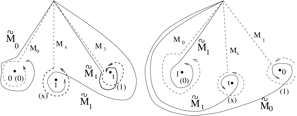
Let M0M_{0}, M1M_{1}, MxM_{x} be the monodromy matrices at z=0,1,xz=0,1,x, for a given basis in the fundamental group of 𝐏1\{0,1,x,∞}{\bf P}^{1}\backslash\{0,1,x,\infty\}. Such basis is chosen as in figure 2.

If

θ0,θx,θ1,θ∞∉𝐙\theta_{0},~\theta_{x},~\theta_{1},~\theta_{\infty}~\not\in{\bf Z}

there is a one to one correspondence between a given choice of monodromy data θ0\theta_{0}, θx\theta_{x}, θ1\theta_{1}, θ∞\theta_{\infty}, tr​(M0​Mx)\hbox{tr}(M_{0}M_{x}), tr​(M0​M1)\hbox{tr}(M_{0}M_{1}), tr​(M1​Mx)\hbox{tr}(M_{1}M_{x}) and a transcendent y⁡(x)y(x). Namely:

y⁡(x)=y⁡(x,θ0,θx,θ1,θ∞,tr​(M0​Mx),tr​(M0​M1),tr​(M1​Mx))y(x)=y\bigl(x;~\theta_{0},\theta_{x},\theta_{1},\theta_{\infty},\hbox{tr}(M_{0}M_{x}),\hbox{tr}(M_{0}M_{1}),\hbox{tr}(M_{1}M_{x})~\bigr) (21)

We prove that such a transcendent has elliptic representations at x=0,1,∞x=0,1,\infty, provided that (14) is satisfied. The three sets of parameters (ν1(i),ν2(i))(\nu_{1}^{(i)},\nu_{2}^{(i)}), i=0,1,∞i=0,1,\infty are functions of the monodromy data θ0\theta_{0}, θx\theta_{x}, θ1\theta_{1}, θ∞\theta_{\infty}, tr​(M0​Mx)\hbox{tr}(M_{0}M_{x}), tr​(M0​M1)\hbox{tr}(M_{0}M_{1}), tr​(M1​Mx)\hbox{tr}(M_{1}M_{x}). Namely, we show that

2​cos⁡(π​ν2(0))=−tr​(M0​Mx),2​cos⁡(π​ν2(1))=−tr​(M1​Mx),2​cos⁡(π​ν2(0))=−tr​(M0​M1)2\cos(\pi\nu_{2}^{(0)})=-\hbox{tr}(M_{0}M_{x}),~~~2\cos(\pi\nu_{2}^{(1)})=-\hbox{tr}(M_{1}M_{x}),~~~2\cos(\pi\nu_{2}^{(0)})=-\hbox{tr}(M_{0}M_{1}) (22)
a(i)=a(i)(ν2(i);θ0,θx,θ1,θ∞,tr(M0Mx),tr(M0M1),tr(M1Mx)),i=0,1,∞a^{(i)}=a^{(i)}\bigl(\nu_{2}^{(i)};\theta_{0},\theta_{x},\theta_{1},\theta_{\infty},\hbox{tr}(M_{0}M_{x}),\hbox{tr}(M_{0}M_{1}),\hbox{tr}(M_{1}M_{x})\bigr),~~~~i=0,1,\infty

The formulas of a(i)a^{(i)} are quite long, so we do not write them here. They depend on the monodromy data through rational, trigonometric and Γ\Gamma-functions. In particular, ν2(i)\nu_{2}^{(i)} enters explicitly. The procedure for computing such formulae is given in the Appendix. We note that the condition ν2(i)∉𝐙\nu_{2}^{(i)}\not\in{\bf Z} is equivalent to tr(Mi​Mj)≠±2(M_{i}M_{j})\neq\pm 2.

Conversely, we prove that a transcendent y⁡(x)y(x) given by its elliptic representation close to one critical point is a transcendent (21) for some monodromy data. This follows from the consideration that the couple (ν1(i),ν2(i))(\nu_{1}^{(i)},\nu_{2}^{(i)}) is given at the critical point x=ix=i, and θ0\theta_{0}, θx\theta_{x}, θ1\theta_{1}, θ∞\theta_{\infty} are fixed by the equation PVI we are considering. From these data we can compute tr​(M0​Mx)\hbox{tr}(M_{0}M_{x}), tr​(M1​Mx)\hbox{tr}(M_{1}M_{x}), tr​(M0​M1)\hbox{tr}(M_{0}M_{1}). One of the traces is −2​cos⁡(π​ν2(i))-2\cos(\pi\nu_{2}^{(i)}), the others depend on ν1(i),ν2(i)\nu_{1}^{(i)},\nu_{2}^{(i)}, θ0\theta_{0}, θx\theta_{x}, θ1\theta_{1}, θ∞\theta_{\infty} through rational, trigonometric and Γ\Gamma-functions. The formulae are rather long, so we refer the reader to the Appendix. In this way the transcendent (21) is obtained. From the monodromy data we compute the couples (ν1(j),ν2(j))(\nu_{1}^{(j)},\nu_{2}^{(j)}) at the other two critical points and we get the the elliptic representation of the initial transcendent at the other critical points. Therefore, the connection problem is solved.

Note that if we start from the elliptic representation at one critical point, say for example x=0x=0, then ν1(0),ν2(0)\nu_{1}^{(0)},\nu_{2}^{(0)} are given. As explained above, we can compute the monodromy data and from them we compute ν2(j)\nu^{(j)}_{2} and a(j)a^{(j)} (then ν1(j)\nu_{1}^{(j)}) at the other two critical points. As already observed, the ambiguity ν1(j)↦ν1(j)+2​k\nu_{1}^{(j)}\mapsto\nu_{1}^{(j)}+2k (kk integer) does not change the elliptic representation. On the other hand, the ambiguities ν2(j)↦ν2(j)+2​N\nu_{2}^{(j)}\mapsto\nu_{2}^{(j)}+2N (NN integer), ν2(j)↦−ν2(j)\nu_{2}^{(j)}\mapsto-\nu_{2}^{(j)} and the ambiguity in the choice 0≤ℜ⁡ν2(j)≤10\leq\Re\nu_{2}^{(j)}\leq 1 or 1≤ℜ⁡ν2(j)≤21\leq\Re\nu_{2}^{(j)}\leq 2, which results from the cosines in (22), is due to the fact that the same transcendent has different elliptic representations in different domains (the choice of ν2(j)\nu_{2}^{(j)} determines the representation and the domain!).

To conclude the discussion of the generic case, some comments about our extension of previous known results are in order. The critical behavior for a class of solutions to the Painlevé 6 equation was found by Jimbo in [15] for generic values of α\alpha, β\beta, γ\gamma δ\delta. A transcendent in this class has behavior:

y⁡(x)=a(0)​x1−σ(0)​(1+O⁡(|x|δ)),x→0,y(x)=a^{(0)}x^{1-\sigma^{(0)}}(1+O(|x|^{\delta})),~~~~x\to 0, (23)
y⁡(x)=1−a(1)​(1−x)1−σ(1)​(1+O⁡(|1−x|δ)),x→1,y(x)=1-a^{(1)}(1-x)^{1-\sigma^{(1)}}(1+O(|1-x|^{\delta})),~~~~x\to 1, (24)
y⁡(x)=a(∞)​x−σ(∞)​(1+O⁡(|x|−δ)),x→∞,y(x)=a^{(\infty)}x^{-\sigma^{(\infty)}}(1+O(|x|^{-\delta})),~~~~x\to\infty, (25)

where δ\delta is a small positive number, a(i)a^{(i)} and σ(i)\sigma^{(i)} are complex numbers such that a(i)≠0a^{(i)}\neq 0 and

0≤ℜ⁡σ(i)<1.0\leq\Re\sigma^{(i)}<1. (26)

We remark that xx converges to the critical points inside a sector with vertex on the corresponding critical point. The connection problem, i.e. the problem of finding the relation among the three pairs (σ(i),a(i))(\sigma^{(i)},a^{(i)}), i=0,1,∞i=0,1,\infty, was solved in [15] for the above class of transcendents using the isomonodromy deformations theory. Actually, a transcendent in the class above coincides with a transcendent (21). In particular

2​cos⁡(π​σ(0))=tr​(M0​Mx),2​cos⁡(π​σ(1))=tr​(M1​Mx),2​cos⁡(π​σ(∞))=tr​(M0​M1)2\cos(\pi\sigma^{(0)})=\hbox{tr}(M_{0}M_{x}),~~~2\cos(\pi\sigma^{(1)})=\hbox{tr}(M_{1}M_{x}),~~~2\cos(\pi\sigma^{(\infty)})=\hbox{tr}(M_{0}M_{1})

and

a(i)=a(i)(σ(i);θ0,θx,θ1,θ∞,tr(M0Mx),tr(M0M1),tr(M1Mx)),i=0,1,∞a^{(i)}=a^{(i)}\bigl(\sigma^{(i)};\theta_{0},\theta_{x},\theta_{1},\theta_{\infty},\hbox{tr}(M_{0}M_{x}),\hbox{tr}(M_{0}M_{1}),\hbox{tr}(M_{1}M_{x})\bigr),~~~~i=0,1,\infty

For the formulas of a(i)a^{(i)} we refer to [15]. The monodromy data are restricted by the following condition, equivalent to (26):

|tr​(Mi​Mj)|≤2,ℜ⁡{tr​(Mi​Mj)}≠−2|\hbox{tr}(M_{i}M_{j})|\leq 2,~~~\Re\{\hbox{tr}(M_{i}M_{j})\}\neq-2 (27)

As explained above, we have shown that the transcendents (21) have elliptic representation. Therefore, Jimbo’s transcendents are included in our class of transcendents obtained by the elliptic representation. Observe that the behaviors (23)–(25) are included in the behaviors (15)–(17) (and (18)–(20)), which hold for any ν2(i)∉(−∞,0]∪{1}∪[2,+∞)\nu_{2}^{(i)}\not\in(-\infty,0]\cup\{1\}\cup[2,+\infty). Therefore the condition (26) is extended to any σ(i)∈𝐂\sigma^{(i)}\in{\bf C} such that σ(i)∉(−∞,0]∪[1,+∞)\sigma^{(i)}\not\in(-\infty,0]\cup[1,+\infty). This corresponds to the fact that we have solved the connection problem for any complex value of tr​(Mi​Mj)\hbox{tr}(M_{i}M_{j}) with the only constraint tr​(Mi​Mj)≠±2\hbox{tr}(M_{i}M_{j})\neq\pm 2. This condition extends (27).

To be more precise, the condition ν2(i)≠1\nu_{2}^{(i)}\neq 1 is equivalent to tr​(M0​Mx)≠2\hbox{tr}(M_{0}M_{x})\neq 2 at x=0x=0; to tr​(M1​Mx)≠2\hbox{tr}(M_{1}M_{x})\neq 2 at x=1x=1; to tr​(M0​M1)≠2\hbox{tr}(M_{0}M_{1})\neq 2 at x=∞x=\infty. Nevertheless, in the case tr​(Mi​Mj)=2\hbox{tr}(M_{i}M_{j})=2 the critical behavior and the solution of the connection problem were achieved by Jimbo. Unfortunately, the condition ν2(i)≠1\nu_{2}^{(i)}\neq 1 which we had to impose to study the elliptic representation (except for non-generic cases like β=γ=1−2​δ=0\beta=\gamma=1-2\delta=0) does not allow us to know the analytic properties and the critical behavior of the elliptic representation in this case. We expect that the properties of u⁡(x)u(x) are such to exactly produce the critical behavior found by Jimbo for tr​(Mi​Mj)=2\hbox{tr}(M_{i}M_{j})=2, but we still have to cover this case.

The condition ν2(i)≠0\nu_{2}^{(i)}\neq 0 (and 2), implies that we can not give the critical behaviors (and the elliptic representation) of (21) at x=0x=0 for tr​(M0​Mx)=−2\hbox{tr}(M_{0}M_{x})=-2; at x=1x=1 for tr​(M1​Mx)=−2\hbox{tr}(M_{1}M_{x})=-2; at x=∞x=\infty for tr​(M0​M1)=−2\hbox{tr}(M_{0}M_{1})=-2. To our knowledge, these cases have not yet been studied in the literature.

To conclude, the results of [15] together with our extension provide the critical behaviors and the solution of the connection problem for the transcendents (21) in the generic case for

 any value of tr​(Mi​Mj)≠−2\hbox{ any value of }\hbox{tr}(M_{i}M_{j})\neq-2

which corresponds to exponents

σ(i)∈𝐂 such that σ(i)∉(−∞,0)∪[1,+∞).\sigma^{(i)}\in{\bf C}\hbox{ such that }\sigma^{(i)}\not\in(-\infty,0)\cup[1,+\infty).

We turn now to the special case β=γ=1−2​δ=0\beta=\gamma=1-2\delta=0, important for its applications to topological filed theory, Frobenius manifolds [5] and quantum cohomology [19] [12]. In this case is fully studied in [11]. We can give a representation of u⁡(x)u(x) in a domain which is wider than the generic case. Namely, at x=0x=0, the domain is

𝒟(r;ν1,ν2):={x∈𝐂0~||x|<r,|e−i​π​ν1(x16)2−ν2|<r,|ei​π​ν1(x16)ν2|<r}{\cal D}(r;\nu_{1},\nu_{2}):=\left\{x\in\tilde{{\bf C}_{0}}~|~|x|<r,~\left|e^{-i\pi\nu_{1}}\left({x\over 16}\right)^{2-\nu_{2}}\right|<r,~\left|e^{i\pi\nu_{1}}\left({x\over 16}\right)^{\nu_{2}}\right|<r\right\}

In this domain v⁡(x)v(x) is holomorphic with convergent expansion

v⁡(x)=∑n≥1an​xn+∑n≥0,m≥1bn​m​xn​[e−i​π​ν1​(x16)2−ν2]m+∑n≥0,m≥1cn​m​xn​[ei​π​ν1​(x16)ν2]mv(x)=\sum_{n\geq 1}a_{n}x^{n}+\sum_{n\geq 0,m\geq 1}b_{nm}x^{n}\left[e^{-i\pi\nu_{1}}\left({x\over 16}\right)^{2-\nu_{2}}\right]^{m}+\sum_{n\geq 0,m\geq 1}c_{nm}x^{n}\left[e^{i\pi\nu_{1}}\left({x\over 16}\right)^{\nu_{2}}\right]^{m}

If ν2\nu_{2} is real, the value ν2=1\nu_{2}=1 is now allowed, namely, the constraint is ν2∉(−∞,0]∪[2,+∞)\nu_{2}\not\in(-\infty,0]\cup[2,+\infty). Therefore, by periodicity of the ℘\wp-function we can assume 0≤ℜ⁡ν2<20\leq\Re\nu_{2}<2, ν2≠0\nu_{2}\neq 0. A similar result holds at x=1x=1 and x=∞x=\infty (see section 8.2).

According to [7], we define 2−x02:=tr​M0​Mx2-x^{2}_{0}:=\hbox{tr}~M_{0}M_{x}, 2−x12:=tr​M1​Mx2-x^{2}_{1}:=\hbox{tr}~M_{1}M_{x}, 2−x∞2:=tr​M0​M12-x^{2}_{\infty}:=\hbox{tr}~M_{0}M_{1}. There is a one to one correspondence between triples (x0,x1,x∞)(x_{0},x_{1},x_{\infty}) (defined up to the change of two signs) and Painlevé transcendents, provided that at most one xix_{i} is zero and not all the xix_{i} are ±2\pm 2 at the same time. Therefore we write y⁡(x)=y⁡(x,x0,x1,x∞)y(x)=y(x;x_{0},x_{1},x_{\infty}). We show that one such transcendent has elliptic representations (half-periods are understood)

y⁡(x,x0,x1,x∞)=℘⁡(ν1(0)​ω1(0)​(x)+ν2(0)​ω2(0)​(x)+v(0)​(x,ν1(0),ν2(0)))+1+x3y(x;x_{0},x_{1},x_{\infty})=\wp\bigl(\nu_{1}^{(0)}\omega_{1}^{(0)}(x)+\nu_{2}^{(0)}\omega_{2}^{(0)}(x)+v^{(0)}(x;\nu_{1}^{(0)},\nu_{2}^{(0)})\bigr)+{1+x\over 3}
=℘⁡(ν1(1)​ω1(1)​(x)+ν2(1)​ω2(1)​(x)+v(1)​(x,ν1(1),ν2(1)))+1+x3=\wp\bigl(\nu_{1}^{(1)}\omega_{1}^{(1)}(x)+\nu_{2}^{(1)}\omega_{2}^{(1)}(x)+v^{(1)}(x;\nu_{1}^{(1)},\nu_{2}^{(1)})\bigr)+{1+x\over 3} (28)
=℘⁡(ν1(∞)​ω1(∞)​(x)+ν2(∞)​ω2(∞)​(x)+v(∞)​(x,ν1(∞),ν2(∞)))+1+x3=\wp\bigl(\nu_{1}^{(\infty)}\omega_{1}^{(\infty)}(x)+\nu_{2}^{(\infty)}\omega_{2}^{(\infty)}(x)+v^{(\infty)}(x;\nu_{1}^{(\infty)},\nu_{2}^{(\infty)})\bigr)+{1+x\over 3} (29)

The parameters ν2(i)\nu_{2}^{(i)} are obtained from

cosπν2(i)=xi22−1,0≤ℜν2(i)≤1,ν2(i)≠0,i=0,1,∞\cos\pi\nu_{2}^{(i)}={x_{i}^{2}\over 2}-1,~~~0\leq\Re\nu_{2}^{(i)}\leq 1,~~~\nu_{2}^{(i)}\neq 0,~~~~i=0,1,\infty

Note that the condition xi≠±2x_{i}\neq\pm 2, i=0,1,∞i=0,1,\infty, corresponds to ν2(i)≠0\nu_{2}^{(i)}\neq 0. The parameter ν1(0)\nu_{1}^{(0)} is obtained by the formula

ei​π​ν1(0)=−i​Γ4​(1−ν2(0)2)2​sin⁡(π​ν2(0))​Γ2​(32−μ−ν2(0)2)​Γ2​(12+μ−ν2(0)2)[2(1−ei​π​ν2(0))−e^{i\pi\nu_{1}^{(0)}}=-{i\Gamma^{4}\left(1-{\nu_{2}^{(0)}\over 2}\right)\over 2\sin(\pi\nu_{2}^{(0)})\Gamma^{2}\left({3\over 2}-\mu-{\nu_{2}^{(0)}\over 2}\right)\Gamma^{2}\left({1\over 2}+\mu-{\nu_{2}^{(0)}\over 2}\right)}\left[2(1-e^{i\pi\nu_{2}^{(0)}})-\right.
−f(x0,x1,x∞)(x∞2−ei​π​ν2(0)x12)]f(x0,x1,x∞)\left.-f(x_{0},x_{1},x_{\infty})(x_{\infty}^{2}-e^{i\pi\nu_{2}^{(0)}}x_{1}^{2})\right]f(x_{0},x_{1},x_{\infty})

where

f⁡(x0,x1,x∞):=4−x02x12+x∞2−x0​x1​x∞,α=(2​μ−1)22f(x_{0},x_{1},x_{\infty}):={4-x_{0}^{2}\over x_{1}^{2}+x_{\infty}^{2}-x_{0}x_{1}x_{\infty}},~~~\alpha={(2\mu-1)^{2}\over 2}

Moreover, exp⁡{−i​π​ν1(1)}\exp\{-i\pi\nu_{1}^{(1)}\}, exp⁡{i​π​ν1(∞)}\exp\{i\pi\nu_{1}^{(\infty)}\} are given by an analogous formula with the substitutions (x0,x1,x∞)↦(x1,x0,x0​x1−x∞)(x_{0},x_{1},x_{\infty})\mapsto(x_{1},x_{0},x_{0}x_{1}-x_{\infty}), ν2(0)↦ν2(1)\nu_{2}^{(0)}\mapsto\nu_{2}^{(1)} and (x0,x1,x∞)↦(x∞,−x1,x0−x1​x∞)(x_{0},x_{1},x_{\infty})\mapsto(x_{\infty},-x_{1},x_{0}-x_{1}x_{\infty}), ν2(0)↦ν2(∞)\nu_{2}^{(0)}\mapsto\nu_{2}^{(\infty)} respectively.

The most general choice of ν2\nu_{2} is 0≤ℜ⁡ν2<20\leq\Re\nu_{2}<2. This corresponds to the fact that the transcendent y⁡(x,x0,x1,x∞)y(x;x_{0},x_{1},x_{\infty}) also has three representations

y⁡(x,x0,x1,x∞)=℘⁡(ν~1(0)​ω1(0)​(x)+ν~2(0)​ω2(0)​(x)+v(0)​(x,ν~1(0),ν~2(0)))+1+x3y(x;x_{0},x_{1},x_{\infty})=\wp\bigl(\tilde{\nu}_{1}^{(0)}\omega_{1}^{(0)}(x)+\tilde{\nu}_{2}^{(0)}\omega_{2}^{(0)}(x)+v^{(0)}(x;\tilde{\nu}_{1}^{(0)},\tilde{\nu}_{2}^{(0)})\bigr)+{1+x\over 3}
=℘⁡(ν~1(1)​ω1(1)​(x)+ν~2(1)​ω2(1)​(x)+v(1)​(x,ν~1(1),ν~2(1)))+1+x3=\wp\bigl(\tilde{\nu}_{1}^{(1)}\omega_{1}^{(1)}(x)+\tilde{\nu}_{2}^{(1)}\omega_{2}^{(1)}(x)+v^{(1)}(x;\tilde{\nu}_{1}^{(1)},\tilde{\nu}_{2}^{(1)})\bigr)+{1+x\over 3}
=℘⁡(ν~1(∞)​ω1(∞)​(x)+ν~2(∞)​ω2(∞)​(x)+v(∞)​(x,ν~1(∞),ν~2(∞)))+1+x3=\wp\bigl(\tilde{\nu}_{1}^{(\infty)}\omega_{1}^{(\infty)}(x)+\tilde{\nu}_{2}^{(\infty)}\omega_{2}^{(\infty)}(x)+v^{(\infty)}(x;\tilde{\nu}_{1}^{(\infty)},\tilde{\nu}_{2}^{(\infty)})\bigr)+{1+x\over 3}

where

cosπν~2(i)=xi22−1,1≤ℜν2(i)<2,i=0,1,∞\cos\pi\tilde{\nu}_{2}^{(i)}={x_{i}^{2}\over 2}-1,~~~1\leq\Re\nu_{2}^{(i)}<2,~~~~i=0,1,\infty

The parameter ν~1(0)\tilde{\nu}_{1}^{(0)} is obtained by the formula

e−i​π​ν~1(0)=i​Γ4​(ν~2(0)2)2​sin⁡(π​ν~2(0))​Γ2​(12−μ+ν~2(0)2)​Γ2​(−12+μ+ν22)[2(1−e−i​π​ν~2(0))−e^{-i\pi\tilde{\nu}^{(0)}_{1}}={i\Gamma^{4}\left({\tilde{\nu}^{(0)}_{2}\over 2}\right)\over 2\sin(\pi\tilde{\nu}_{2}^{(0)})\Gamma^{2}\left({1\over 2}-\mu+{\tilde{\nu}_{2}^{(0)}\over 2}\right)\Gamma^{2}\left(-{1\over 2}+\mu+{\nu_{2}\over 2}\right)}\left[2(1-e^{-i\pi\tilde{\nu}_{2}^{(0)}})-\right.
−f(x0,x1,x∞)(x∞2−e−i​π​ν~2(0)x12)]f(x0,x1,x∞).\left.-f(x_{0},x_{1},x_{\infty})(x_{\infty}^{2}-e^{-i\pi\tilde{\nu}^{(0)}_{2}}x_{1}^{2})\right]f(x_{0},x_{1},x_{\infty}).

exp⁡{i​π​ν~1(1)}\exp\{i\pi\tilde{\nu}_{1}^{(1)}\}, exp⁡{−i​π​ν~1(∞)}\exp\{-i\pi\tilde{\nu}_{1}^{(\infty)}\} are given by an analogous formula with the substitutions (x0,x1,x∞)↦(x1,x0,x0​x1−x∞)(x_{0},x_{1},x_{\infty})\mapsto(x_{1},x_{0},x_{0}x_{1}-x_{\infty}), ν~2(0)↦ν~2(1)\tilde{\nu}_{2}^{(0)}\mapsto\tilde{\nu}_{2}^{(1)} and (x0,x1,x∞)↦(x∞,−x1,x0−x1​x∞)(x_{0},x_{1},x_{\infty})\mapsto(x_{\infty},-x_{1},x_{0}-x_{1}x_{\infty}), ν~2(0)↦ν~2(∞)\tilde{\nu}_{2}^{(0)}\mapsto\tilde{\nu}_{2}^{(\infty)} respectively.

The formulae above have limits for ν2=1,1±2​μ+2​m\nu_{2}=1,1\pm 2\mu+2m, mm integer. They are listed in subsection 8.2.

Conversely, a transcendent

y⁡(x)=℘⁡(ν1​ω1(0)​(x)+ν2​ω2(0)​(x)+v(0)​(x,ν1,ν2))+1+x3, at ​x=0y(x)=\wp\bigl({\nu}_{1}\omega_{1}^{(0)}(x)+{\nu}_{2}\omega_{2}^{(0)}(x)+v^{(0)}(x;{\nu}_{1},{\nu}_{2})\bigr)+{1+x\over 3},~~~\hbox{ at }x=0 (30)

coincides with y⁡(x,x0,x1,x∞)y(x;~x_{0},x_{1},x_{\infty}), with the following monodromy data.

If 0≤ℜ⁡ν2≤10\leq\Re\nu_{2}\leq 1:

x0=2​cos⁡(π2​ν2)x_{0}=2\cos\left({\pi\over 2}\nu_{2}\right)
x1=[4−ν2​2​ei​π2​ν1f⁡(ν2,μ)​G​(ν2,μ)+G⁡(ν2,μ)4−ν2​2​ei​π2​ν1]x_{1}=\left[{4^{-\nu_{2}}~2~e^{i{\pi\over 2}\nu_{1}}\over f(\nu_{2},\mu)G(\nu_{2},\mu)}+{G(\nu_{2},\mu)\over 4^{-\nu_{2}}~2~e^{i{\pi\over 2}\nu_{1}}}\right]
x∞=[4−ν2​2​ei​π2​(ν1−ν2)f⁡(ν2,μ)​G​(ν2,μ)+G⁡(ν2,μ)4−ν2​2​ei​π2​(ν1−ν2)]x_{\infty}=\left[{4^{-\nu_{2}}~2~e^{i{\pi\over 2}(\nu_{1}-\nu_{2})}\over f(\nu_{2},\mu)G(\nu_{2},\mu)}+{G(\nu_{2},\mu)\over 4^{-\nu_{2}}~2~e^{i{\pi\over 2}(\nu_{1}-\nu_{2})}}\right]

where

f⁡(ν2,μ)=−2​sin2⁡(π2​ν2)cos⁡(π​ν2)+cos⁡(2​π​μ),G⁡(ν2,μ)=4−ν2​2​Γ​(1−ν22)2Γ⁡(32−μ−ν22)​Γ​(12+μ−ν22)f(\nu_{2},\mu)=-{2\sin^{2}\left({\pi\over 2}\nu_{2}\right)\over\cos(\pi\nu_{2})+\cos(2\pi\mu)},~~~G(\nu_{2},\mu)=4^{-\nu_{2}}~2~{\Gamma\left(1-{\nu_{2}\over 2}\right)^{2}\over\Gamma\left({3\over 2}-\mu-{\nu_{2}\over 2}\right)\Gamma\left({1\over 2}+\mu-{\nu_{2}\over 2}\right)}

If 1≤ℜ⁡ν2<21\leq\Re\nu_{2}<2:

x0=2​cos⁡(π2​ν2)x_{0}=2\cos\left({\pi\over 2}\nu_{2}\right)
x1=[e−i​π2​ν141−ν2​2​f​(ν2,μ)​G1​(ν2,μ)+41−ν2​2​G1​(ν2,μ)e−i​π2​ν1]x_{1}=\left[{e^{-i{\pi\over 2}\nu_{1}}\over 4^{1-\nu_{2}}~2~f(\nu_{2},\mu)G_{1}(\nu_{2},\mu)}+{4^{1-\nu_{2}}~2~G_{1}(\nu_{2},\mu)\over e^{-i{\pi\over 2}\nu_{1}}}\right]
x∞=[ei​π2​(ν2−ν1)41−ν2​2​f​(ν2,μ)​G1​(ν2,μ)+41−ν2​2​G1​(ν2,μ)ei​π2​(ν2−ν1)]x_{\infty}=\left[{e^{i{\pi\over 2}(\nu_{2}-\nu_{1})}\over 4^{1-\nu_{2}}~2~f(\nu_{2},\mu)G_{1}(\nu_{2},\mu)}+{4^{1-\nu_{2}}~2~G_{1}(\nu_{2},\mu)\over e^{i{\pi\over 2}(\nu_{2}-\nu_{1})}}\right]

where

G1​(ν2,μ)=141−ν2​2​Γ​(ν22)2Γ⁡(12−μ+ν22)​Γ​(−12+μ+ν22)G_{1}(\nu_{2},\mu)={1\over 4^{1-\nu_{2}}~2}{\Gamma\left({\nu_{2}\over 2}\right)^{2}\over\Gamma\left({1\over 2}-\mu+{\nu_{2}\over 2}\right)\Gamma\left(-{1\over 2}+\mu+{\nu_{2}\over 2}\right)}

After computing the monodromy data, we can write the elliptic representations of y⁡(x,x0,x1,x∞)y(x;x_{0},x_{1},x_{\infty}) at x=1x=1 and x=∞x=\infty, namely (28), (29). Since they are the elliptic representations at x=1x=1, x=∞x=\infty of (30), we have solved the connection problem for (30).

We observed that there is a one to one correspondence between Painlevé transcendents and triples of monodromy data (x0,x1,x∞)(x_{0},x_{1},x_{\infty}), defined up to the change of two signs, satisfying xi≠±2x_{i}\neq\pm 2, i=0,1,∞i=0,1,\infty, i.e. ν2(i)≠0\nu_{2}^{(i)}\neq 0 (and 2), and at most one xi=0x_{i}=0. The cases when these conditions are not satisfied are studied in [23]. However, if xi=±2x_{i}=\pm 2 (namely the trace is −2-2) the problem of finding the critical behavior at the corresponding critical point x=ix=i is still open (except when all the three xix_{i} are ±2\pm 2: in this case there is a one-parameter class of solutions called Chazy solutions in [23]). We conclude that the results of our paper (and [11]), plus the results of [23] cover all the possible transcendents, except the special case when one or two xix_{i} are ±2\pm 2. We plan to cover this last case soon.

Finally, we expect that in all non-generic cases we can solve the connection problem and express the parameters ν1\nu_{1}, ν2\nu_{2} in terms of monodromy data. From the conceptual point of view nothing should change with respect to [15] [7] [11] and the present paper; but the technical details may require a long time for computations.

2 The Elliptic Representation

We derive the elliptic form for the general Painlevé 6 equation. We follow [8]. Let

u=∫∞yd​λλ​(λ−1)​(λ−x)u=\int_{\infty}^{y}~{d\lambda\over\sqrt{\lambda(\lambda-1)(\lambda-x)}} (31)

We observe that

d​ud​x=∂u∂y​d​yd​x+∂u∂x=1y​(y−1)​(y−x)​d​yd​x+∂u∂x{du\over dx}={\partial u\over\partial y}~{dy\over dx}+{\partial u\over\partial x}={1\over\sqrt{y(y-1)(y-x)}}~{dy\over dx}+{\partial u\over\partial x}

from which we compute

d2​ud​x2+2​x−1x⁡(x−1)​d​ud​x+u4​x​(x−1)={d^{2}u\over dx^{2}}+{2x-1\over x(x-1)}{du\over dx}+{u\over 4x(x-1)}=
=1y​(y−1)​(y−x)​[d2​yd​x2+(1x+1x−1+1y−x)​d​yd​x−12​(1y+1y−1+1y−x)​(d​yd​x)2]={1\over\sqrt{y(y-1)(y-x)}}\left[{d^{2}y\over dx^{2}}+\left({1\over x}+{1\over x-1}+{1\over y-x}\right)~{dy\over dx}-{1\over 2}\left({1\over y}+{1\over y-1}+{1\over y-x}\right)~\left({dy\over dx}\right)^{2}\right]
+∂2u∂x2+2​x−1x⁡(x−1)​∂u∂x+u4​x​(x−1)+{\partial^{2}u\over\partial x^{2}}+{2x-1\over x(x-1)}~{\partial u\over\partial x}+{u\over 4x(x-1)}

By direct calculation we have:

∂2u∂x2+2​x−1x⁡(x−1)​∂u∂x+u4​x​(x−1)=−12​y​(y−1)​(y−x)x⁡(x−1)​1(y−x)2{\partial^{2}u\over\partial x^{2}}+{2x-1\over x(x-1)}~{\partial u\over\partial x}+{u\over 4x(x-1)}=-{1\over 2}{\sqrt{y(y-1)(y-x)}\over x(x-1)}~{1\over(y-x)^{2}}

Therefore, y⁡(x)y(x) satisfies PVI if and only if

d2​ud​x2+2​x−1x⁡(x−1)​d​ud​x+u4​x​(x−1)=y​(y−1)​(y−x)2​x2​(1−x)2​[2​α+2​β​xy2+γ​x−1(y−1)2+(δ−12)​x⁡(x−1)(y−x)2]{d^{2}u\over dx^{2}}+{2x-1\over x(x-1)}~{du\over dx}+{u\over 4x(x-1)}={\sqrt{y(y-1)(y-x)}\over 2x^{2}(1-x)^{2}}~\left[2\alpha+2\beta{x\over y^{2}}+\gamma{x-1\over(y-1)^{2}}+\left(\delta-{1\over 2}\right){x(x-1)\over(y-x)^{2}}\right] (32)

We invert the function u=u⁡(y)u=u(y) by observing that we are dealing with an elliptic integral. Therefore, we write

y=f⁡(u,x)y=f(u,x)

where f⁡(u,x)f(u,x) is an elliptic function of uu. This implies that

∂y∂u=y​(y−1)​(y−x){\partial y\over\partial u}=\sqrt{y(y-1)(y-x)}

The above equality allows us to rewrite (32) in the following way:

x⁡(1−x)​d2​ud​x2+(1−2​x)​d​ud​x−14​u=12​x​(1−x)​∂∂u​ψ​(u,x),x(1-x)~{d^{2}u\over dx^{2}}+(1-2x)~{du\over dx}-{1\over 4}~u={1\over 2x(1-x)}~{\partial\over\partial u}\psi(u,x), (33)

where

ψ⁡(u,x):=2​α​f​(u,x)−2​β​xf⁡(u,x)+2​γ​1−xf⁡(u,x)−1+(1−2​δ)​x⁡(x−1)f⁡(u,x)−x\psi(u,x):=2\alpha f(u,x)-2\beta{x\over f(u,x)}+2\gamma{1-x\over f(u,x)-1}+(1-2\delta){x(x-1)\over f(u,x)-x}

The last step concerns the form of f⁡(u,x)f(u,x). We observe that 4​λ​(λ−1)​(λ−x)4\lambda(\lambda-1)(\lambda-x) is not in Weierstrass canonical form. We change variable:

λ=t+1+x3,\lambda=t+{1+x\over 3},

and we get the Weierstrass form:

4​λ​(λ−1)​(λ−x)=4​t3−g2​t−g3,g2=43​(1−x+x2),g3:=427​(x−2)​(2​x−1)​(1+x)4\lambda(\lambda-1)(\lambda-x)=4t^{3}-g_{2}t-g_{3},~~~~g_{2}={4\over 3}(1-x+x^{2}),~~~~g_{3}:={4\over 27}(x-2)(2x-1)(1+x)

Thus

u2=∫∞y−1+x3d​t4​t3−g2​t−g3{u\over 2}=\int_{\infty}^{y-{1+x\over 3}}~{dt\over\sqrt{4t^{3}-g_{2}t-g_{3}}}

which implies

f⁡(u,x)=𝒫⁡(u2,ω1,ω2)+1+x3f(u,x)={\cal P}\left({u\over 2};\omega_{1},\omega_{2}\right)+{1+x\over 3}

We still need to explain what are the half periods ω1\omega_{1}, ω2\omega_{2}. In order to do that, we first observe that the Weierstrass form is

4​t3−g2​t−g3=4​(t−e1)​(t−e2)​(t−e3)4t^{3}-g_{2}t-g_{3}=4(t-e_{1})(t-e_{2})(t-e_{3})

where

e1=2−x3,e2=2​x−13,e3=−1+x3.e_{1}={2-x\over 3},~~~e_{2}={2x-1\over 3},~~~e_{3}=-{1+x\over 3}.

Therefore

g:=e1−e2=1,κ2:=e2−e3e1−e3=x,κ′2:=1−κ2=1−xg:=\sqrt{e_{1}-e_{2}}=1,~~~{\kappa}^{2}:={e_{2}-e_{3}\over e_{1}-e_{3}}=x,~~~{{\kappa}^{\prime}}^{2}:=1-{\kappa}^{2}=1-x

We identify e1=℘⁡(ω1)e_{1}=\wp(\omega_{1}), e2=℘⁡(ω1+ω2)e_{2}=\wp(\omega_{1}+\omega_{2}), e3=℘⁡(ω2)e_{3}=\wp(\omega_{2}). Therefore, the half-periods are

ω1=1g​∫01d​ξ(1−ξ2)​(1−κ2​ξ2)=∫01d​ξ(1−ξ2)​(1−x​ξ2)=𝐊⁡(x)\omega_{1}={1\over g}\int_{0}^{1}~{d\xi\over\sqrt{(1-\xi^{2})(1-\kappa^{2}\xi^{2})}}=\int_{0}^{1}~{d\xi\over\sqrt{(1-\xi^{2})(1-x\xi^{2})}}={\bf K}(x)
ω2=ig​∫01d​ξ(1−ξ2)​(1−κ′2​ξ2)=i​∫01d​ξ(1−ξ2)​(1−(1−x)​ξ2)=i​𝐊​(1−x)\omega_{2}={i\over g}\int_{0}^{1}~{d\xi\over\sqrt{(1-\xi^{2})(1-{\kappa^{\prime}}^{2}\xi^{2})}}=i~\int_{0}^{1}~{d\xi\over\sqrt{(1-\xi^{2})(1-(1-x)\xi^{2})}}=i{\bf K}(1-x)

The elliptic integral 𝐊⁡(x){\bf K}(x) coincides, up to a factor, with the hyper-geometric function F⁡(12,12,1,x)F\left({1\over 2},{1\over 2},1;x\right), whose convergent series for |x|<1|x|<1 is:

F⁡(12,12,1,x)=∑n=0∞[(12)n]2(n!)2​xn.F\left({1\over 2},{1\over 2},1;x\right)=\sum_{n=0}^{\infty}{\left[\left({1\over 2}\right)_{n}\right]^{2}\over(n!)^{2}}x^{n}.

Namely:

𝐊⁡(x)=π2​F​(12,12,1,x){\bf K}(x)={\pi\over 2}~F\left({1\over 2},{1\over 2},1;x\right)

Moreover, 𝐊⁡(x){\bf K}(x) and 𝐊⁡(1−x){\bf K}(1-x) are two linearly independent solutions of the hyper-geometric equation

x⁡(1−x)​ω′′+(1−2​x)​ω′−14​ω=0.x(1-x)\omega^{\prime\prime}+(1-2x)\omega^{\prime}-{1\over 4}\omega=0.

Observe that for |arg​(x)|<π|\hbox{arg}(x)|<\pi:

−π​F​(12,12,1,1−x)=F⁡(12,12,1,x)​ln⁡(x)+F1​(x)-\pi F\left({1\over 2},{1\over 2},1;1-x\right)=F\left({1\over 2},{1\over 2},1;x\right)\ln(x)+F_{1}(x)

where

F1​(x):=∑n=0∞[(12)n]2(n!)2​2​[ψ⁡(n+12)−ψ⁡(n+1)]​xn,F_{1}(x):=\sum_{n=0}^{\infty}{\left[\left({1\over 2}\right)_{n}\right]^{2}\over(n!)^{2}}2\left[\psi(n+{1\over 2})-\psi(n+1)\right]x^{n},
ψ⁡(z)=dd​z​ln⁡Γ⁡(z),ψ⁡(12)=−γ−2​ln​2,ψ⁡(1)=−γ,ψ⁡(a+n)=ψ⁡(a)+∑l=0n−11a+l.\psi(z)={d\over dz}\ln\Gamma(z),~~~\psi\left({1\over 2}\right)=-\gamma-2\ln 2,~~~\psi(1)=-\gamma,~~~\psi(a+n)=\psi(a)+\sum_{l=0}^{n-1}{1\over a+l}.

Therefore

ω2​(x)=−i2​[F⁡(12,12,1,x)​ln⁡(x)+F1​(x)]\omega_{2}(x)=-{i\over 2}[F\left({1\over 2},{1\over 2},1;x\right)\ln(x)+F_{1}(x)]

In the following we use sometimes the abbreviation F⁡(x)F(x) for F⁡(12,12,1,x)F\left({1\over 2},{1\over 2},1;x\right). The series of F⁡(x)F(x) and F1​(x)F_{1}(x) converge for |x|<1|x|<1.

Let

ℒ⁡(u):=x⁡(1−x)​d2​ud​x2+(1−2​x)​d​ud​x−14​u{\cal L}(u):=x(1-x){d^{2}u\over dx^{2}}+(1-2x){du\over dx}-{1\over 4}u

The PVI equation becomes

ℒ(u)=12​x​(1−x)∂∂u{2α[℘(u2;ω1,ω2)−e3]−2βx℘⁡(u2,ω1,ω2)−e3+{\cal L}(u)={1\over 2x(1-x)}{\partial\over\partial u}\left\{2\alpha\left[\wp\left({u\over 2};\omega_{1},\omega_{2}\right)-e_{3}\right]-2\beta{x\over\wp\left({u\over 2};\omega_{1},\omega_{2}\right)-e_{3}}+\right.
+2γ1−x℘⁡(u2,ω1,ω2)−e1+(1−2δ)x⁡(1−x)℘⁡(u2,ω1,ω2)−e2}\left.+2\gamma{1-x\over\wp\left({u\over 2};\omega_{1},\omega_{2}\right)-e_{1}}+(1-2\delta){x(1-x)\over\wp\left({u\over 2};\omega_{1},\omega_{2}\right)-e_{2}}\right\} (34)

We recall that

1℘⁡(u2)−e3=1(e1−e3)​(e2−e3)​[℘⁡(u2+ω2)−e3]{1\over\wp\left({u\over 2}\right)-e_{3}}={1\over(e_{1}-e_{3})(e_{2}-e_{3})}\left[\wp\left({u\over 2}+\omega_{2}\right)-e_{3}\right]
1℘⁡(u2)−e1=1(e1−e2)​(e1−e3)​[℘⁡(u2+ω1)−e1]{1\over\wp\left({u\over 2}\right)-e_{1}}={1\over(e_{1}-e_{2})(e_{1}-e_{3})}\left[\wp\left({u\over 2}+\omega_{1}\right)-e_{1}\right]
1℘⁡(u2)−e2=1(e1−e2)​(e3−e2)​[℘⁡(u2+ω1+ω2)−e2].{1\over\wp\left({u\over 2}\right)-e_{2}}={1\over(e_{1}-e_{2})(e_{3}-e_{2})}\left[\wp\left({u\over 2}+\omega_{1}+\omega_{2}\right)-e_{2}\right].

We observe also that e1−e3=1e_{1}-e_{3}=1, e2−e3=xe_{2}-e_{3}=x, e1−e2=1−xe_{1}-e_{2}=1-x. Therefore, (34) becomes:

ℒ(u)=12​x​(1−x)[2α∂∂u℘(u2)−2β∂∂u℘(u2+ω2)+{\cal L}(u)={1\over 2x(1-x)}\left[2\alpha{\partial\over\partial u}\wp\left({u\over 2}\right)-2\beta{\partial\over\partial u}\wp\left({u\over 2}+\omega_{2}\right)+\right.
+2γ∂∂u℘(u2+ω1)+(1−2δ)∂∂u℘(u2+ω1+ω2)]\left.+2\gamma{\partial\over\partial u}\wp\left({u\over 2}+\omega_{1}\right)+(1-2\delta){\partial\over\partial u}\wp\left({u\over 2}+\omega_{1}+\omega_{2}\right)\right] (35)

3 Proof of Theorem 1

For technical reason it is convenient to introduce the following definitions:

𝒟1(r;ν1,ν2):={x∈𝐂0~ such that |x|<r,|e−i​π​ν1161−ν2x1−ν2|<r,|ei​π​ν116ν2xν2|<r}{\cal D}_{1}(r;\nu_{1},\nu_{2}):=\left\{x\in\widetilde{{\bf C}_{0}}~\hbox{ such that }|x|<r,\left|{e^{-i\pi\nu_{1}}\over 16^{1-\nu_{2}}}x^{1-\nu_{2}}\right|<r,\left|{e^{i\pi\nu_{1}}\over 16^{\nu_{2}}}x^{\nu_{2}}\right|<r\right\} (36)
𝒟2(r;ν1,ν2):={x∈𝐂0~ such that |x|<r,|e−i​π​ν1162−ν2x2−ν2|<r,|ei​π​ν116ν2−1xν2−1|<r}{\cal D}_{2}(r;\nu_{1},\nu_{2}):=\left\{x\in\widetilde{{\bf C}_{0}}~\hbox{ such that }|x|<r,\left|{e^{-i\pi\nu_{1}}\over 16^{2-\nu_{2}}}x^{2-\nu_{2}}\right|<r,\left|{e^{i\pi\nu_{1}}\over 16^{\nu_{2}-1}}x^{\nu_{2}-1}\right|<r\right\} (37)

Note that 𝒟1​(r,ν1,ν2)≡𝒟⁡(r,ν1,ν2){\cal D}_{1}(r;\nu_{1},\nu_{2})\equiv{\cal D}(r;\nu_{1},\nu_{2}) in (2) and 𝒟2​(r,ν1,ν2)≡𝒟⁡(r,−ν1,2−ν2){\cal D}_{2}(r;\nu_{1},\nu_{2})\equiv{\cal D}(r;-\nu_{1},2-\nu_{2}). Let

τ⁡(x):=ω2​(x)ω1​(x)=1π​(arg⁡x−i​ln⁡|x|16)+O⁡(x)\tau(x):={\omega_{2}(x)\over\omega_{1}(x)}={1\over\pi}(\arg x-i\ln{|x|\over 16})+O(x)

be the modular parameter of the elliptic function, obtained expanding ω1​(x)\omega_{1}(x), ω2​(x)\omega_{2}(x) at x=0x=0. We expand the r.h.s of (35) in Fourier series. We are dealing with Weierstrass ℘\wp-functions of the form ℘⁡(u2+ε1​ω1+ε2​ω2)\wp\left({u\over 2}+\varepsilon_{1}\omega_{1}+\varepsilon_{2}\omega_{2}\right), where εi∈{0,1}\varepsilon_{i}\in\{0,1\}, i=1,2i=1,2. Due to periodicity of ℘\wp we are going to expand

℘⁡(u2+[ε1+2​N1]​ω1+[ε2+2​N2]​ω2),εi∈{0,1},Ni∈𝐙,i=1,2\wp\left({u\over 2}+[\varepsilon_{1}+2N_{1}]~\omega_{1}+[\varepsilon_{2}+2N_{2}]~\omega_{2}\right),~~~~\varepsilon_{i}\in\{0,1\},~~~N_{i}\in{\bf Z},~~~i=1,2

As it is well known [33], the Fourier expansion of the ℘\wp-function is

℘⁡(z,ω1,ω2)=(π2​ω1)2​[−13+1sin2⁡(π​z2​ω1)+8​∑n≥1n​e2​i​π​n​τ1−e2​i​π​n​τ​[1−cos⁡(n​π​zω1)]], for ​ℑ⁡τ>|ℑ⁡(z2​ω1)|\wp(z;\omega_{1},\omega_{2})=\left({\pi\over 2\omega_{1}}\right)^{2}~\left[-{1\over 3}+{1\over\sin^{2}\left({\pi z\over 2\omega_{1}}\right)}+8\sum_{n\geq 1}{ne^{2i\pi n\tau}\over 1-e^{2i\pi n\tau}}~\left[1-\cos\left({n\pi z\over\omega_{1}}\right)\right]\right],~~~\hbox{ for }\Im\tau>\left|\Im\left({z\over 2\omega_{1}}\right)\right|

Therefore, the expansion is possible provided that

|ℑ⁡(u⁡(x)4​ω1​(x)+ε1+2​N12+ε2+2​N22​τ​(x))|<ℑ⁡τ⁡(x)\left|\Im\left({u(x)\over 4\omega_{1}(x)}+{\varepsilon_{1}+2N_{1}\over 2}+{\varepsilon_{2}+2N_{2}\over 2}~\tau(x)\right)\right|<\Im\tau(x) (38)

We observe that for x→0x\to 0

ℑ⁡τ⁡(x)=−1π​ln⁡|x|16+O⁡(x)→+∞\Im\tau(x)=-{1\over\pi}\ln{|x|\over 16}+O(x)\to+\infty

The condition (38) becomes

−ℑ⁡τ<12​ℑ​ν1+12​[ε2+2​N2+ℜ⁡ν2]​ℑ​τ+12​ℑ​ν2​ℜ​τ+ℑ⁡(v2​ω1)<ℑ⁡τ-\Im\tau<{1\over 2}\Im\nu_{1}+{1\over 2}[\varepsilon_{2}+2N_{2}+\Re\nu_{2}]~\Im\tau+{1\over 2}\Im\nu_{2}~\Re\tau+\Im\left({v\over 2\omega_{1}}\right)<\Im\tau (39)

If ν2\nu_{2} is real, we divide by ℑ⁡τ\Im\tau, we let x→0x\to 0 and we obtain

−2−2​N2−ε2<ν2<2−2​N2−ϵ2-2-2N_{2}-\varepsilon_{2}<\nu_{2}<2-2N_{2}-\epsilon_{2}

provided that v⁡(x)v(x) is bounded. In general, (39) becomes

(ℜ⁡ν2+2+ε2+2​N2)​ln⁡|x|16−[π​ℑ⁡ν1+ℑ⁡(π​vω1)]+O⁡(x)(\Re\nu_{2}+2+\varepsilon_{2}+2N_{2})\ln{|x|\over 16}-\left[\pi\Im\nu_{1}+\Im\left({\pi v\over\omega_{1}}\right)\right]+O(x)
≤ℑ⁡ν2​arg⁡x≤\leq\Im\nu_{2}\arg x\leq
(ℜ⁡ν2−2+ε2+2​N2)​ln⁡|x|16−[π​ℑ⁡ν1+ℑ⁡(π​vω1)]+O⁡(x)(\Re\nu_{2}-2+\varepsilon_{2}+2N_{2})\ln{|x|\over 16}-\left[\pi\Im\nu_{1}+\Im\left({\pi v\over\omega_{1}}\right)\right]+O(x) (40)

In the domain defined by the above condition, and |x|<1|x|<1, we do the Fourier expansion as follows

∂∂u​℘​(u2+[ε1+2​N1]​ω1+[ε2+2​N2]​ω2)={\partial\over\partial u}\wp\left({u\over 2}+[\varepsilon_{1}+2N_{1}]\omega_{1}+[\varepsilon_{2}+2N_{2}]\omega_{2}\right)=
=π38​ω13​{8​∑n≥1n2​e2​i​π​n​τ1−e2​i​π​n​τ​sin⁡[π​n​(u2​ω1+ϵ1+(ϵ2+2​N2)​τ)]−cos⁡[π2​(u2​ω1+ϵ1+(ϵ2+2​N2)​τ)]sin3⁡[π2​(u2​ω1+ϵ1+(ϵ2+2​N2)​τ)]}={\pi^{3}\over 8\omega_{1}^{3}}\left\{8\sum_{n\geq 1}{n^{2}e^{2i\pi n\tau}\over 1-e^{2i\pi n\tau}}\sin\left[\pi n\left({u\over 2\omega_{1}}+\epsilon_{1}+(\epsilon_{2}+2N_{2})\tau\right)\right]-{\cos\left[{\pi\over 2}\left({u\over 2\omega_{1}}+\epsilon_{1}+(\epsilon_{2}+2N_{2})\tau\right)\right]\over\sin^{3}\left[{\pi\over 2}\left({u\over 2\omega_{1}}+\epsilon_{1}+(\epsilon_{2}+2N_{2})\tau\right)\right]}\right\}
=i​π32​ω13​{ei​f⁡(x)2+e−i​f⁡(x)2[ei​f⁡(x)2−e−i​f⁡(x)2]3−∑n≥1n2​e2​i​π​n​τ1−e2​i​π​n​τ​[ei​n​f​(x)−e−i​n​f​(x)]}={i\pi^{3}\over 2\omega_{1}^{3}}\left\{{e^{i{f(x)\over 2}}+e^{-i{f(x)\over 2}}\over\left[e^{i{f(x)\over 2}}-e^{-i{f(x)\over 2}}\right]^{3}}-\sum_{n\geq 1}{n^{2}e^{2i\pi n\tau}\over 1-e^{2i\pi n\tau}}\left[e^{inf(x)}-e^{-inf(x)}\right]\right\} (41)

where

ei​f​(x)=exp⁡{i​π​[(ν1+ε1)+(ν2+ε2+2​N2)​τ​(x)+v⁡(x)ω1​(x)]}e^{if(x)}=\exp\left\{i\pi\left[(\nu_{1}+\varepsilon_{1})+(\nu_{2}+\varepsilon_{2}+2N_{2})\tau(x)+{v(x)\over\omega_{1}(x)}\right]\right\}

Note that N1N_{1} does not appear in the expansion. So, we can take N1=0N_{1}=0 in the following.

Now we make the further assumption that

|ei​f​(x)|<1\left|e^{if(x)}\right|<1 (42)

and we rewrite (41) as follows:

i​π32​ω13​{e2​i​f​(x)+ei​f​(x)[ei​f​(x)−1]3−∑n≥1n2​ei​π​n​[−(ν1+ε1)+(2−ν2−ε2−2​N2)​τ−vω1]1−e2​π​n​τ​[e2​i​n​f​(x)−1]}{i\pi^{3}\over 2\omega_{1}^{3}}\left\{{e^{2if(x)}+e^{if(x)}\over\left[e^{if(x)}-1\right]^{3}}-\sum_{n\geq 1}{n^{2}e^{i\pi n\left[-(\nu_{1}+\varepsilon_{1})+(2-\nu_{2}-\varepsilon_{2}-2N_{2})\tau-{v\over\omega_{1}}\right]}\over 1-e^{2\pi n\tau}}~\left[e^{2inf(x)}-1\right]\right\}

Due to (42), the denominator in the first term does not vanish, so that the expansion has no poles. The condition (42) is more restrictive than (40) and yields:

(ℜ⁡ν2+ε2+2​N2)​ln⁡|x|16−[π​ℑ⁡ν1+ℑ⁡(π​vω1)]+O⁡(x)(\Re\nu_{2}+\varepsilon_{2}+2N_{2})\ln{|x|\over 16}-\left[\pi\Im\nu_{1}+\Im\left({\pi v\over\omega_{1}}\right)\right]+O(x)
≤ℑ⁡ν2​arg⁡x≤\leq\Im\nu_{2}\arg x\leq
(ℜ⁡ν2−2+ε2+2​N2)​ln⁡|x|16−[π​ℑ⁡ν1+ℑ⁡(π​vω1)]+O⁡(x)(\Re\nu_{2}-2+\varepsilon_{2}+2N_{2})\ln{|x|\over 16}-\left[\pi\Im\nu_{1}+\Im\left({\pi v\over\omega_{1}}\right)\right]+O(x) (43)

We observe that, for any complex number CC,

ei​π​C​τ​(x)=h​(x)C​[x16]C,e^{i\pi C\tau(x)}=h(x)^{C}~\left[{x\over 16}\right]^{C},

where

h⁡(x):=eC⁡(F1​(x)F⁡(x)+4​ln⁡2)=1+O⁡(x),x→0h(x):=e^{C\left({F_{1}(x)\over F(x)}+4\ln 2\right)}=1+O(x),~~~~x\to 0

Therefore,

∂∂u​℘​(u2+(ε1+2​N1)​ω1+(ε2+2​N2)​ω2)=i​π32​ω13​{A2+A(A−1)3−∑n≥1n2​Bn1−h​(x)2​n​(x16)2​n​(A2​n−1)}{\partial\over\partial u}\wp\left({u\over 2}+(\varepsilon_{1}+2N_{1})\omega_{1}+(\varepsilon_{2}+2N_{2})\omega_{2}\right)={i\pi^{3}\over 2\omega_{1}^{3}}\left\{{A^{2}+A\over\left(A-1\right)^{3}}-\sum_{n\geq 1}{n^{2}B^{n}\over 1-h(x)^{2n}\left({x\over 16}\right)^{2n}}\left(A^{2n}-1\right)\right\}

where

A=A⁡(x,ei​π​ν1​(x16)ν2+ϵ2+2​N2​ei​π​vω1):=h​(x)ν2+ε2+2​N2​ei​π​(ε1+ν1)​(x16)ν2+ε2+2​N2​ei​π​vω1A=A\left(x,e^{i\pi\nu_{1}}\left({x\over 16}\right)^{\nu_{2}+\epsilon_{2}+2N_{2}}e^{i\pi{v\over\omega_{1}}}\right):=h(x)^{\nu_{2}+\varepsilon_{2}+2N_{2}}e^{i\pi(\varepsilon_{1}+\nu_{1})}\left({x\over 16}\right)^{\nu_{2}+\varepsilon_{2}+2N_{2}}e^{i{\pi v\over\omega_{1}}} (44)
B=B⁡(x,e−i​π​ν1​(x16)2−ν2−ε2−2​N2​e−i​π​vω1):=h​(x)2−ν2−ε2−2​N2​e−i​π​(ν1+ε1)​(x16)2−ν2−ε2−2​N2​e−i​π​vω1B=B\left(x,e^{-i\pi\nu_{1}}\left({x\over 16}\right)^{2-\nu_{2}-\varepsilon_{2}-2N_{2}}e^{-i\pi{v\over\omega_{1}}}\right):=h(x)^{2-\nu_{2}-\varepsilon_{2}-2N_{2}}e^{-i\pi(\nu_{1}+\varepsilon_{1})}\left({x\over 16}\right)^{2-\nu_{2}-\varepsilon_{2}-2N_{2}}e^{-i\pi{v\over\omega_{1}}} (45)

In the r.h.s. of equation (35), we have four ℘\wp-functions with different arguments. We recall that we can take N1=0N_{1}=0. As for N2N_{2}, it can be different in each ℘\wp-function. There are only two possibilities in order for the four resulting domains (43) to intersect: the ℘\wp-functions must be

℘⁡(u2+2​N2​ω2),℘⁡(u2+ω1+2​N2​ω2),℘⁡(u2+ω2+2​N2′​ω2),℘⁡(u2+ω1+ω2+2​N2′​ω2),\wp\left({u\over 2}+2N_{2}\omega_{2}\right),~~~~~~\wp\left({u\over 2}+\omega_{1}+2N_{2}\omega_{2}\right),~~~\wp\left({u\over 2}+\omega_{2}+2N^{\prime}_{2}\omega_{2}\right),~~~~~~\wp\left({u\over 2}+\omega_{1}+\omega_{2}+2N^{\prime}_{2}\omega_{2}\right),

and

(a):N2′=N2(a):~~~~~N_{2}^{\prime}=N_{2}

or

(b):N2′=N2−1(b):~~~~~N_{2}^{\prime}=N_{2}-1

Thus, the r.h.s. of (35) is expanded in Fourier series if |x|<1|x|<1, in the following domains.

Case (a):

(ℜ⁡ν2+2​N)​ln​|x|16−[π​ℑ​ν1+ℑ⁡(π​vω1)]+O⁡(x)<ℑ⁡ν2​arg​x<(\Re\nu_{2}+2N)\ln{|x|\over 16}-\left[\pi\Im\nu_{1}+\Im\left({\pi v\over\omega_{1}}\right)\right]+O(x)<\Im\nu_{2}\arg x<
<(ℜν2−1+2N)ln|x|16−[πℑν1+ℑ(π​vω1)]+O(x), for N2′=N2=:N<(\Re\nu_{2}-1+2N)\ln{|x|\over 16}-\left[\pi\Im\nu_{1}+\Im\left({\pi v\over\omega_{1}}\right)\right]+O(x),~~~~\hbox{ for }N_{2}^{\prime}=N_{2}=:N (46)

Case (b):

(ℜ⁡ν2−1+2​N)​ln​|x|16−[π​ℑ​ν1+ℑ⁡(π​vω1)]+O⁡(x)<ℑ⁡ν2​arg​x<(\Re\nu_{2}-1+2N)\ln{|x|\over 16}-\left[\pi\Im\nu_{1}+\Im\left({\pi v\over\omega_{1}}\right)\right]+O(x)<\Im\nu_{2}\arg x<
<(ℜν2−2+2N)ln|x|16−[πℑν1+ℑ(π​vω1)]+O(x), for N2′+1=N2=:N<(\Re\nu_{2}-2+2N)\ln{|x|\over 16}-\left[\pi\Im\nu_{1}+\Im\left({\pi v\over\omega_{1}}\right)\right]+O(x),~~~~\hbox{ for }N_{2}^{\prime}+1=N_{2}=:N (47)

Note that if ℑ⁡ν2=0\Im\nu_{2}=0 any value of arg⁡(x)\arg(x) is allowed, but dividing the previous expressions by ln⁡|x|\ln|x| and letting x→0x\to 0 we have

−2​N<ν2<1−2​N​ for (a),1−2​N<ν2<2−2​N​ for (b)-2N<\nu_{2}<1-2N\hbox{ for (a)},~~~~~1-2N<\nu_{2}<2-2N\hbox{ for (b)}

provided that v⁡(x)v(x) is bounded fort x→0x\to 0. Taking (44) (45) into account in the two cases, we conclude that:

In case (a), for N2′=N2=NN_{2}^{\prime}=N_{2}=N, the following powers appear in the r.h.s. of (35):

x2−ν2−2​N,xν2+2​N,x1−ν2−2​N,x1+ν2+2​Nx^{2-\nu_{2}-2N},~~~x^{\nu_{2}+2N},~~~x^{1-\nu_{2}-2N},~~~x^{1+\nu_{2}+2N}

The dominant powers are then

xν2+2​N,x1−ν2−2​Nx^{\nu_{2}+2N},~~~x^{1-\nu_{2}-2N}

and we can write (35) as;

ℒ⁡(u)=12​x​(1−x)​ℱ​(x,e−i​π​ν1​(x16)1−ν2−2​N​e−i​π​vω1,ei​π​ν1​(x16)ν2+2​N​ei​π​vω1){\cal L}(u)={1\over 2x(1-x)}{\cal F}\left(x,e^{-i\pi\nu_{1}}\left({x\over 16}\right)^{1-\nu_{2}-2N}e^{-i\pi{v\over\omega_{1}}},e^{i\pi\nu_{1}}\left({x\over 16}\right)^{\nu_{2}+2N}e^{i\pi{v\over\omega_{1}}}\right)

on the domain defined by |x|<1|x|<1 and (46), assuming that v⁡(x)v(x) is bounded.

In case (b), for N2′+1=N2=NN_{2}^{\prime}+1=N_{2}=N, the following powers appear in the r.h.s. of (35):

x2−ν2−2​N,xν2+2​N,x3−ν2−2​N,xν2−1+2​Nx^{2-\nu_{2}-2N},~~~x^{\nu_{2}+2N},~~~x^{3-\nu_{2}-2N},~~~x^{\nu_{2}-1+2N}

The dominant powers are then

x2−ν2−2​N,xν2−1+2​Nx^{2-\nu_{2}-2N},~~~x^{\nu_{2}-1+2N}

and we can write (35) as;

ℒ⁡(u)=12​x​(1−x)​ℱ​(x,e−i​π​ν1​(x16)2−ν2−2​N​e−i​π​vω1,ei​π​ν1​(x16)ν2−1+2​N​ei​π​vω1){\cal L}(u)={1\over 2x(1-x)}{\cal F}\left(x,e^{-i\pi\nu_{1}}\left({x\over 16}\right)^{2-\nu_{2}-2N}e^{-i\pi{v\over\omega_{1}}},e^{i\pi\nu_{1}}\left({x\over 16}\right)^{\nu_{2}-1+2N}e^{i\pi{v\over\omega_{1}}}\right)

on the domain defined by |x|<1|x|<1 and (47), assuming that v⁡(x)v(x) is bounded.

Let ϵ<1\epsilon<1 be sufficiently small: in both cases, ℱ⁡(x,y,z){\cal F}(x,y,z) is holomorphic for |x|,|y|,|z|<ϵ|x|,|y|,|z|<\epsilon and ℱ⁡(0,0,0)=0{\cal F}(0,0,0)=0. In (a) we decompose

ℱ⁡(x,e−i​π​ν1​(x16)1−ν2−2​N​e−i​π​vω1,ei​π​ν1​(x16)ν2+2​N​ei​π​vω1)={\cal F}\left(x,e^{-i\pi\nu_{1}}\left({x\over 16}\right)^{1-\nu_{2}-2N}e^{-i\pi{v\over\omega_{1}}},e^{i\pi\nu_{1}}\left({x\over 16}\right)^{\nu_{2}+2N}e^{i\pi{v\over\omega_{1}}}\right)=
=ℱ⁡(x,e−i​π​ν1​(x16)1−ν2−2​N,ei​π​ν1​(x16)ν2+2​N)+𝒢⁡(x,e−i​π​ν1​(x16)1−ν2−2​N,ei​π​ν1​(x16)ν2+2​N,v)={\cal F}\left(x,e^{-i\pi\nu_{1}}\left({x\over 16}\right)^{1-\nu_{2}-2N},e^{i\pi\nu_{1}}\left({x\over 16}\right)^{\nu_{2}+2N}\right)+{\cal G}\left(x,e^{-i\pi\nu_{1}}\left({x\over 16}\right)^{1-\nu_{2}-2N},e^{i\pi\nu_{1}}\left({x\over 16}\right)^{\nu_{2}+2N},v\right)

where

𝒢⁡(x,e−i​π​ν1​(x16)1−ν2−2​N,ei​π​ν1​(x16)ν2+2​N,v):={\cal G}\left(x,e^{-i\pi\nu_{1}}\left({x\over 16}\right)^{1-\nu_{2}-2N},e^{i\pi\nu_{1}}\left({x\over 16}\right)^{\nu_{2}+2N},v\right):=
ℱ⁡(x,e−i​π​ν1​(x16)1−ν2−2​N​e−i​π​vω1,ei​π​ν1​(x16)ν2+2​N​ei​π​vω1)−{\cal F}\left(x,e^{-i\pi\nu_{1}}\left({x\over 16}\right)^{1-\nu_{2}-2N}e^{-i\pi{v\over\omega_{1}}},e^{i\pi\nu_{1}}\left({x\over 16}\right)^{\nu_{2}+2N}e^{i\pi{v\over\omega_{1}}}\right)-
−ℱ⁡(x,e−i​π​ν1​(x16)1−ν2−2​N,ei​π​ν1​(x16)ν2+2​N)-{\cal F}\left(x,e^{-i\pi\nu_{1}}\left({x\over 16}\right)^{1-\nu_{2}-2N},e^{i\pi\nu_{1}}\left({x\over 16}\right)^{\nu_{2}+2N}\right)

We note that ℒ⁡(u)=ℒ⁡(u0+2​v){\cal L}(u)={\cal L}(u_{0}+2v)=ℒ⁡(u0)+2​ℒ​(v)≡2​ℒ​(v){\cal L}(u_{0})+2{\cal L}(v)\equiv 2{\cal L}(v). Let us put

w⁡(x):=x​dd​x​v​(x)w(x):=x{d\over dx}v(x)

Equation (35) becomes the system

{x​d​vd​x=wx​d​wd​x=Φ+Ψ\left\{\matrix{x{dv\over dx}=w\cr\cr x{dw\over dx}=\Phi+\Psi}\right.

where

Φ=Φ⁡(x,e−i​π​ν1​(x16)1−ν2−2​N,ei​π​ν1​(x16)ν2+2​N):=\Phi=\Phi\left(x,e^{-i\pi\nu_{1}}\left({x\over 16}\right)^{1-\nu_{2}-2N},e^{i\pi\nu_{1}}\left({x\over 16}\right)^{\nu_{2}+2N}\right):=
=14​(1−x)2​ℱ​(x,e−i​π​ν1​(x16)1−ν2−2​N,ei​π​ν1​(x16)ν2+2​N)={1\over 4(1-x)^{2}}{\cal F}\left(x,e^{-i\pi\nu_{1}}\left({x\over 16}\right)^{1-\nu_{2}-2N},e^{i\pi\nu_{1}}\left({x\over 16}\right)^{\nu_{2}+2N}\right)

and

Ψ=Ψ⁡(x,e−i​π​ν1​(x16)1−ν2−2​N,ei​π​ν1​(x16)ν2+2​N,v,w):=\Psi=\Psi\left(x,e^{-i\pi\nu_{1}}\left({x\over 16}\right)^{1-\nu_{2}-2N},e^{i\pi\nu_{1}}\left({x\over 16}\right)^{\nu_{2}+2N},v,w\right):=
=x⁡(w+v/4)1−x+14​(1−x)2​𝒢​(x,e−i​π​ν1​(x16)1−ν2−2​N,ei​π​ν1​(x16)ν2+2​N,v)={x(w+v/4)\over 1-x}+{1\over 4(1-x)^{2}}{\cal G}\left(x,e^{-i\pi\nu_{1}}\left({x\over 16}\right)^{1-\nu_{2}-2N},e^{i\pi\nu_{1}}\left({x\over 16}\right)^{\nu_{2}+2N},v\right)

In the same way, in case (b) we obtain a similar system, where

Φ=Φ⁡(x,e−i​π​ν1​(x16)2−ν2−2​N,ei​π​ν1​(x16)ν2−1+2​N)\Phi=\Phi\left(x,e^{-i\pi\nu_{1}}\left({x\over 16}\right)^{2-\nu_{2}-2N},e^{i\pi\nu_{1}}\left({x\over 16}\right)^{\nu_{2}-1+2N}\right)
Ψ=Ψ⁡(x,e−i​π​ν1​(x16)2−ν2−2​N,ei​π​ν1​(x16)ν2−1+2​N,v,w)\Psi=\Psi\left(x,e^{-i\pi\nu_{1}}\left({x\over 16}\right)^{2-\nu_{2}-2N},e^{i\pi\nu_{1}}\left({x\over 16}\right)^{\nu_{2}-1+2N},v,w\right)

By construction, in both cases Φ⁡(x,y,z)\Phi(x,y,z) and Ψ⁡(x,y,z,v,w)\Psi(x,y,z,v,w) are holomorphic of their arguments for |x|,|y|,|z|,|v|,|w|<ϵ|x|,|y|,|z|,|v|,|w|<\epsilon for sufficiently small ϵ<1\epsilon<1 (assuming v⁡(x)v(x) bounded in a neighborhood of x=0x=0). Moreover

Φ⁡(0,0,0)=Ψ⁡(0,0,0,v,w)=Ψ⁡(x,y,z,0,0)=0\Phi(0,0,0)=\Psi(0,0,0,v,w)=\Psi(x,y,z,0,0)=0

We complete the proof of the theorem in case (a). Case (b) is analogous. We reduce the system of differential equations to a system of integral equations

w(x)=∫L⁡(x)1s{Φ(s,e−i​π​ν1(s16)1−ν2−2​N,ei​π​ν1(s16)ν2+2​N)+w(x)=\int_{L(x)}{1\over s}\left\{\Phi(s,e^{-i\pi\nu_{1}}\left({s\over 16}\right)^{1-\nu_{2}-2N},e^{i\pi\nu_{1}}\left({s\over 16}\right)^{\nu_{2}+2N})+\right.
+Ψ(s,e−i​π​ν1(s16)1−ν2−2​N,ei​π​ν1(s16)ν2+2​N,v(s),w(s))}ds\left.+\Psi(s,e^{-i\pi\nu_{1}}\left({s\over 16}\right)^{1-\nu_{2}-2N},e^{i\pi\nu_{1}}\left({s\over 16}\right)^{\nu_{2}+2N},v(s),w(s))\right\}~ds
v⁡(x)=∫L⁡(x)1s​w​(s)​𝑑sv(x)=\int_{L(x)}{1\over s}w(s)~ds

The point xx and the path of integration are chosen to belong to the domain where |x||x|, |e−i​π​ν1161−ν2−2​N​x1−ν2−2​N||{e^{-i\pi\nu_{1}}\over 16^{1-\nu_{2}-2N}}x^{1-\nu_{2}-2N}|, |ei​π​ν116ν2+2​N​xν2+2​N||{e^{i\pi\nu_{1}}\over 16^{\nu_{2}+2N}}x^{\nu_{2}+2N}|, |v⁡(x)||v(x)|, |w⁡(x)||w(x)| are less than ϵ\epsilon, in such a way that Φ\Phi and Ψ\Psi are holomorphic. That such a domain is not empty will be shown below. In particular, we’ll show that if we require that |x|<r|x|<r, |e−i​π​ν1161−ν2​x1−ν2|<r|{e^{-i\pi\nu_{1}}\over 16^{1-\nu_{2}}}x^{1-\nu_{2}}|<r, |ei​π​ν116ν2​xν2|<r|{e^{i\pi\nu_{1}}\over 16^{\nu_{2}}}x^{\nu_{2}}|<r, where r<ϵr<\epsilon is small enough, also the solutions of the integral equations |v⁡(x)||v(x)| and |w⁡(x)||w(x)| are less than ϵ\epsilon. Such a domain is contained in (46).

We choose the path of integration L⁡(x)L(x) connecting 0 to xx, defined by

arg⁡(s)=arg⁡(x)+ℜ⁡ν2+2​N−ν∗ℑ⁡ν2​log⁡|s||x|,0<|s|≤|x|,ν∗∈𝐂\arg(s)=\arg(x)+{\Re\nu_{2}+2N-\nu^{*}\over\Im\nu_{2}}\log{|s|\over|x|},~~~0<|s|\leq|x|,~~~\nu^{*}\in{\bf C}

If xx belongs to the domain (46) in case (a) and to (47) in case (b), than the path does not leave the domain when s→0s\to 0, provided that 0≤ν∗≤10\leq\nu^{*}\leq 1 in case (a), or 1≤ν∗≤21\leq\nu^{*}\leq 2 in case (b). If ℑ⁡ν2=0\Im\nu_{2}=0 we take the radial path arg⁡s=arg⁡x\arg s=\arg x, 0<|s|≤|x|0<|s|\leq|x|, namely ν∗=ν2\nu^{*}=\nu_{2}. The parameterization of the path is

s=ρ​ei​{arg⁡x+ℜ⁡ν2+2​N−ν∗ℑ⁡ν2​log⁡ρ|x|},0<ρ≤|x|s=\rho~e^{i\left\{\arg x+{\Re\nu_{2}+2N-\nu^{*}\over\Im\nu_{2}}\log{\rho\over|x|}\right\}},~~~~0<\rho\leq|x|

therefore

|d​s|=P⁡(ν2+2​N,ν∗)​d​ρ,P⁡(ν2+2​N,ν∗):=1+(ℜ⁡ν2+2​N−ν∗ℑ⁡ν2)2|ds|=P(\nu_{2}+2N,\nu^{*})~d\rho,~~~~~P(\nu_{2}+2N,\nu^{*}):=\sqrt{1+\left({\Re\nu_{2}+2N-\nu^{*}\over\Im\nu_{2}}\right)^{2}}

For any complex numbers AA, BB we have

∫L⁡(x)1|s|​(|s|+|A​s1−ν2−2​N|+|B​sν2+2​N|)n|𝑑s|≤P⁡(ν2+2​N,ν∗)n​min⁡(ν∗,1−ν∗)​(|x|+|A​x1−ν2−2​N|+|B​xν2+2​N|)n\int_{L(x)}{1\over|s|}\left(|s|+|As^{1-\nu_{2}-2N}|+|Bs^{\nu_{2}+2N}|\right)^{n}~|ds|\leq{P(\nu_{2}+2N,\nu^{*})\over n\min(\nu^{*},1-\nu^{*})}\left(|x|+|Ax^{1-\nu_{2}-2N}|+|Bx^{\nu_{2}+2N}|\right)^{n} (48)

The quantity min⁡(ν∗,1−ν∗)\min(\nu^{*},1-\nu^{*}) is substituted by min⁡(ν∗−1,2−ν∗)\min(\nu^{*}-1,2-\nu^{*}) in case (b). To prove (48) we observe that on L⁡(x)L(x) we have

|sν2+2​N+α|=|xν2+2​N+α|​|s|ν∗+α|x|ν∗+α,∀α∈𝐂.|s^{\nu_{2}+2N+\alpha}|=|x^{\nu_{2}+2N+\alpha}|{|s|^{\nu^{*}+\alpha}\over|x|^{\nu^{*}+\alpha}},~~~~\forall\alpha\in{\bf C}.

Therefore

∫L⁡(x)1|s|​|s|i​|A​s1−ν2−2​N|j​|B​sν2+2​N|k​|𝑑s|=\int_{L(x)}{1\over|s|}|s|^{i}|As^{1-\nu_{2}-2N}|^{j}|Bs^{\nu_{2}+2N}|^{k}~|ds|=
|A​x1−ν2−2​N|j​|B​xν2+2​N|k|x|(1−ν∗)​j​|x|ν∗​k​P​(ν2+2​N,ν∗)​∫0|x|d​ρ​ρi−1+(1−ν∗)​j+ν∗​k{|Ax^{1-\nu_{2}-2N}|^{j}~|Bx^{\nu_{2}+2N}|^{k}\over|x|^{(1-\nu^{*})j}~|x|^{\nu^{*}k}}~P(\nu_{2}+2N,\nu^{*})\int_{0}^{|x|}d\rho~\rho^{i-1+(1-\nu^{*})j+\nu^{*}k}
=P⁡(ν2+2​N,ν∗)i+j⁡(1−ν∗)+k​ν∗​|x|i​|A​x1−ν2−2​N|j​|B​xν2+2​N|k={P(\nu_{2}+2N,\nu^{*})\over i+j(1-\nu^{*})+k\nu^{*}}|x|^{i}~|Ax^{1-\nu_{2}-2N}|^{j}~|Bx^{\nu_{2}+2N}|^{k}
≤P⁡(ν2+2​N,ν∗)(i+j+k)​min⁡(ν∗,1−ν∗)​|x|i​|A​x1−ν2−2​N|j​|B​xν2+2​N|k\leq{P(\nu_{2}+2N,\nu^{*})\over(i+j+k)\min(\nu^{*},1-\nu^{*})}|x|^{i}~|Ax^{1-\nu_{2}-2N}|^{j}~|Bx^{\nu_{2}+2N}|^{k}

from which (48) follows, provided that 0<ν∗<10<\nu^{*}<1. For ℑ⁡ν2=0\Im\nu_{2}=0, this yields again 0<ν2<10<\nu_{2}<1.

We observe that a solution of the integral equations is also a solution of the differential equations, by virtue of the following lemma:

Lemma 1: Let f⁡(x)f(x) be a holomorphic function in the domain |x|<ϵ|x|<\epsilon, |A​x1−ν2−2​N|<ϵ|Ax^{1-\nu_{2}-2N}|<\epsilon, |B​xν2+2​N|<ϵ|Bx^{\nu_{2}+2N}|<\epsilon, such that f⁡(x)=O⁡(|x|+|A​x1−ν2−2​N|+|B​xν2+2​N|)f(x)=O(|x|+|Ax^{1-\nu_{2}-2N}|+|Bx^{\nu_{2}+2N}|), A,B∈𝐂A,B\in{\bf C}. Let L⁡(x)L(x) be the path of integration defined above for 0<ν∗<10<\nu^{*}<1 and

F⁡(x):=∫L⁡(x)1s​f​(s)​𝑑sF(x):=\int_{L(x)}{1\over s}f(s)~ds

Then, F⁡(x)F(x) is holomorphic on the domain and d​F​(x)d​x=1x​f​(x){dF(x)\over dx}={1\over x}f(x)

The same holds for a function f⁡(x)=O⁡(|x|+|A​x2−ν2−2​N|+|B​xν2−1+2​N|)f(x)=O(|x|+|Ax^{2-\nu_{2}-2N}|+|Bx^{\nu_{2}-1+2N}|) in the domain |x|<ϵ|x|<\epsilon, |A​x2−ν2−2​N|<ϵ|Ax^{2-\nu_{2}-2N}|<\epsilon, |B​xν2−1+2​N|<ϵ|Bx^{\nu_{2}-1+2N}|<\epsilon ( L⁡(x)L(x) being defined for 1<ν∗<21<\nu^{*}<2).

Proof: We give the proof in case (a). We choose a point x+Δ​xx+\Delta x close to xx and we prove that ∫L⁡(x)−∫L⁡(x+Δ​x)=∫xx+Δ​x\int_{L(x)}-\int_{L(x+\Delta x)}=\int_{x}^{x+\Delta x}, where the last integral is on a segment from xx to x+Δ​xx+\Delta x. We consider a small disk URU_{R} centered at x=0x=0 of small radius R<|x|R<|x| and the points xR:=L⁡(x)∩URx_{R}:=L(x)\cap U_{R}, xR′:=L⁡(x+Δ​x)∩URx^{\prime}_{R}:=L(x+\Delta x)\cap U_{R}. Since the integral of f/sf/s on a finite close curve (not containing 0) is zero we have:

(∫L⁡(x)−∫L⁡(x+Δ​x)−∫xx+Δ​x)dsf⁡(s)s=(∫L⁡(xR)−∫L⁡(xR′)−∫γ⁡(xR,xR′))dsf⁡(s)s\left(\int_{L(x)}-\int_{L(x+\Delta x)}-\int_{x}^{x+\Delta x}\right)ds~{f(s)\over s}=\left(\int_{L(x_{R})}-\int_{L(x^{\prime}_{R})}-\int_{\gamma(x_{R},x^{\prime}_{R})}\right)ds~{f(s)\over s} (49)

The last integral is on the arc γ⁡(xR,xR′)\gamma(x_{R},x^{\prime}_{R}) from xRx_{R} to xR′x^{\prime}_{R} on the circle |s|=R|s|=R. We have also kept into account the obvious fact that L⁡(xR)L(x_{R}) is contained in L⁡(x)L(x) and L⁡(xR′)L(x^{\prime}_{R}) is contained in L⁡(x+Δ​x)L(x+\Delta x). We then take R→0R\to 0 and we prove that the r.h.s. of (49) vanishes.

Taking into account that f⁡(x)=O⁡(|x|+|A​x1−ν2−2​N|+|B​xν2+2​N|)f(x)=O(|x|+|Ax^{1-\nu_{2}-2N}|+|Bx^{\nu_{2}+2N}|) and (48) we have

|∫L⁡(xR)1s​f​(s)​𝑑s|≤∫L⁡(xR)1|s|​O​(|s|+|A​s1−ν2−2​N|+|B​sν2+2​N|)​|𝑑s|\left|\int_{L(x_{R})}{1\over s}f(s)~ds\right|\leq\int_{L(x_{R})}{1\over|s|}O(|s|+|As^{1-\nu_{2}-2N}|+|Bs^{\nu_{2}+2N}|)~|ds|
≤P⁡(ν2+2​N,ν∗)min⁡(ν∗,1−ν∗)​O​(|xR|+|A​xR1−ν2−2​N|+|B​xRν2+2​N|)=\leq{P(\nu_{2}+2N,\nu^{*})\over\min(\nu^{*},1-\nu^{*})}O(|x_{R}|+|Ax_{R}^{1-\nu_{2}-2N}|+|Bx_{R}^{\nu_{2}+2N}|)=
=P⁡(ν2+2​N,ν∗)min⁡(ν∗,2−ν∗)​O​(Rmin⁡{ν∗,1−ν∗})={P(\nu_{2}+2N,\nu^{*})\over\min(\nu^{*},2-\nu^{*})}~O(R^{\min\{\nu^{*},1-\nu^{*}\}})

The last step follows from |xRν2+2​N|=|xν2+2​N||x|ν∗​Rν∗|x_{R}^{\nu_{2}+2N}|={|x^{\nu_{2}+2N}|\over|x|^{\nu^{*}}}R^{\nu^{*}}. So the integral vanishes for R→0R\to 0. The same is proved for ∫L⁡(x+Δ​x)\int_{L(x+\Delta x)}. As for the integral on the arc we have

|arg⁡xR−arg⁡xR′|=|arg⁡x−arg⁡(x+Δ​x)+ℜ⁡ν2+2​N−ν∗ℑ⁡ν2​log​|1+Δ​xx|||\arg x_{R}-\arg x^{\prime}_{R}|=\left|\arg x-\arg(x+\Delta x)+{\Re\nu_{2}+2N-\nu^{*}\over\Im\nu_{2}}\log\left|1+{\Delta x\over x}\right|\right|

or |arg⁡xR−arg⁡xR′|=|arg⁡x−arg⁡(x+Δ​x)||\arg x_{R}-\arg x^{\prime}_{R}|=\left|\arg x-\arg(x+\Delta x)\right| if ℑ⁡ν2=0\Im\nu_{2}=0. This is independent of RR, therefore the length of the arc is O⁡(R)O(R) and

|∫γ⁡(xR,xR′)1|s|​|f⁡(s)|​|𝑑s||=O⁡(Rmin⁡{ν∗,1−ν∗})→0​ for ​R→0\left|\int_{\gamma(x_{R},x^{\prime}_{R})}{1\over|s|}|f(s)|~|ds|\right|=O(R^{\min\{\nu^{*},1-\nu^{*}\}})\to 0\hbox{ for }R\to 0

□\Box

Now we prove a fundamental lemma.

Lemma 2: For any N∈𝐙N\in{\bf Z} and for any complex ν1\nu_{1}, ν2\nu_{2} such that

ν2∉(−∞,−2N]∪{1−2N}∪[2−2N,+∞)\nu_{2}\not\in(-\infty,-2N]\cup\{1-2N\}\cup[2-2N,+\infty)

there exists a sufficiently small rN<1r_{N}<1 such that the system of integral equations has a solution v1​(x,ν1,ν2+2​N)v_{1}(x;\nu_{1},\nu_{2}+2N) holomorphic in the domain 𝒟1​(rN,ν1,ν2+2​N){\cal D}_{1}(r_{N};\nu_{1},\nu_{2}+2N) defined in (36). Moreover, there exists a positive constant M1​(ν2+2​N)M_{1}(\nu_{2}+2N) depending on ν2+2​N\nu_{2}+2N such that

|v1​(x,ν1,ν2+2​N)|≤M1​(ν2+2​N)​(|x|+|e−i​π​ν1161−ν2−2​N​x1−ν2−2​N|+|ei​π​ν116ν2+2​N​xν2+2​N|)|v_{1}(x;\nu_{1},\nu_{2}+2N)|\leq M_{1}(\nu_{2}+2N)\left(|x|+\left|{e^{-i\pi\nu_{1}}\over 16^{1-\nu_{2}-2N}}x^{1-\nu_{2}-2N}\right|+\left|{e^{i\pi\nu_{1}}\over 16^{\nu_{2}+2N}}x^{\nu_{2}+2N}\right|\right)

in 𝒟1​(r,ν1,ν2){\cal D}_{1}(r;\nu_{1},\nu_{2}).

The system of integral equations has another solution v2​(x,ν1,ν2+2​N)v_{2}(x;\nu_{1},\nu_{2}+2N) holomorphic in 𝒟2​(r,ν1,ν2){\cal D}_{2}(r;\nu_{1},\nu_{2}) defined in (37). There exists a positive constant M2​(ν2+2​N)M_{2}(\nu_{2}+2N) such that

|v2​(x,ν1,ν2+2​N)|≤M2​(ν2+2​N)​(|x|+|e−i​π​ν1162−ν2−2​N​x2−ν2−2​N|+|ei​π​ν116ν2−1+2​N​xν2−1+2​N|)|v_{2}(x;\nu_{1},\nu_{2}+2N)|\leq M_{2}(\nu_{2}+2N)\left(|x|+\left|{e^{-i\pi\nu_{1}}\over 16^{2-\nu_{2}-2N}}x^{2-\nu_{2}-2N}\right|+\left|{e^{i\pi\nu_{1}}\over 16^{\nu_{2}-1+2N}}x^{\nu_{2}-1+2N}\right|\right)

in 𝒟2​(r,ν1,ν2){\cal D}_{2}(r;\nu_{1},\nu_{2}).

Note that 𝒟i​(rN,ν1,ν2+2​N)=𝒟i​(rN,ν1+2​N1,ν2+2​N){\cal D}_{i}(r_{N};\nu_{1},\nu_{2}+2N)={\cal D}_{i}(r_{N};\nu_{1}+2N_{1},\nu_{2}+2N), i=1,2i=1,2, for any N1∈𝐙N_{1}\in{\bf Z}. To prove Lemma 2 we need some sub-lemmas

Sub-Lemma 1: Let Φ⁡(x,y,z)\Phi(x,y,z) and Ψ⁡(x,y,z,v,w)\Psi(x,y,z,v,w) be two holomorphic functions of their arguments for |x|,|y|,|z|,|v|,|w|<ϵ|x|,|y|,|z|,|v|,|w|<\epsilon, satisfying

Φ⁡(0,0,0)=0,Ψ⁡(0,0,0,v,w)=Ψ⁡(x,y,z,0,0)=0\Phi(0,0,0)=0,~~~~\Psi(0,0,0,v,w)=\Psi(x,y,z,0,0)=0

Then, there exists a constant c>0c>0 such that:

|Φ⁡(x,y,z)|≤c⁡(|x|+|y|+|z|)\left|\Phi(x,y,z)\right|\leq c~\left(|x|+|y|+|z|\right) (50)
|Ψ⁡(x,y,z,v,w)|≤c⁡(|x|+|y|+|z|)\left|\Psi(x,y,z,v,w)\right|\leq c~\left(|x|+|y|+|z|\right) (51)
|Ψ⁡(x,y,z,v2,w2)−Ψ⁡(x,y,z,v1,w1)|≤c⁡(|x|+|y|+|z|)​(|v2−v1|+|w2−w1|)\left|\Psi(x,y,z,v_{2},w_{2})-\Psi(x,y,z,v_{1},w_{1})\right|\leq c\left(|x|+|y|+|z|\right)~\left(|v_{2}-v_{1}|+|w_{2}-w_{1}|\right) (52)

for |x|,|y|,|z|,|v|,|w|<ϵ|x|,|y|,|z|,|v|,|w|<\epsilon.

Proof: Let’s proof (51).

Ψ⁡(x,y,z,v,w)=∫01dd​λ​Ψ​(λ​x,λ​y,λ​z,v,w)​𝑑λ\Psi(x,y,z,v,w)=\int_{0}^{1}~{d\over d\lambda}\Psi(\lambda x,\lambda y,\lambda z,v,w)~d\lambda
x​∫01∂Ψ∂x​(λ​x,λ​y,λ​z,v,w)​𝑑λ+y​∫01∂Ψ∂y​(λ​x,λ​y,λ​z,v,w)​𝑑λ+z​∫01∂Ψ∂z​(λ​x,λ​y,λ​z,v,w)​𝑑λx~\int_{0}^{1}{\partial\Psi\over\partial x}(\lambda x,\lambda y,\lambda z,v,w)~d\lambda~+~y\int_{0}^{1}{\partial\Psi\over\partial y}(\lambda x,\lambda y,\lambda z,v,w)~d\lambda~+~z\int_{0}^{1}{\partial\Psi\over\partial z}(\lambda x,\lambda y,\lambda z,v,w)~d\lambda

Moreover, for δ\delta small:

∂Ψ∂x​(λ​x,λ​y,λ​z,v,w)=∫|ζ−λ​x|=δΨ⁡(ζ,λ​y,λ​z,v,w)(ζ−λ​x)2​d​ζ2​π​i{\partial\Psi\over\partial x}(\lambda x,\lambda y,\lambda z,v,w)=\int_{|\zeta-\lambda x|=\delta}~{\Psi(\zeta,\lambda y,\lambda z,v,w)\over(\zeta-\lambda x)^{2}}~{d\zeta\over 2\pi i}

which implies that ∂Ψ∂x{\partial\Psi\over\partial x} is holomorphic and bounded when its arguments are less than ϵ\epsilon. The same holds true for ∂Ψ∂y{\partial\Psi\over\partial y} and ∂Ψ∂z{\partial\Psi\over\partial z}. This proves (51), cc being a constant which bounds |∂Ψ∂x|\left|{\partial\Psi\over\partial x}\right|, |∂Ψ∂y|\left|{\partial\Psi\over\partial y}\right| |∂Ψ∂z|\left|{\partial\Psi\over\partial z}\right|. The inequality (50) is proved in the same way. We turn to (52). First we prove that for |x|,|y|,|z|,|v1|,|w1|,|v2|,|w2|<ϵ|x|,|y|,|z|,|v_{1}|,|w_{1}|,|v_{2}|,|w_{2}|<\epsilon there exist two holomorphic and bounded functions ψ1​(x,y,z,v1,w1,v2,w2)\psi_{1}(x,y,z,v_{1},w_{1},v_{2},w_{2}), ψ2​(x,y,z,v1,w1,v2,w2)\psi_{2}(x,y,z,v_{1},w_{1},v_{2},w_{2}) such that

Ψ⁡(x,y,z,v2,w2)−Ψ⁡(x,y,z,v1,w1)\Psi(x,y,z,v_{2},w_{2})-\Psi(x,y,z,v_{1},w_{1})
=(v2−v1)​ψ1​(x,y,z,v1,w1,v2,w2)+(w1−w2)​ψ2​(x,y,z,v1,w1,v2,w2)=(v_{2}-v_{1})~\psi_{1}(x,y,z,v_{1},w_{1},v_{2},w_{2})+(w_{1}-w_{2})~\psi_{2}(x,y,z,v_{1},w_{1},v_{2},w_{2}) (53)

In order to prove this, we write

Ψ⁡(x,y,z,v2,w2)−Ψ⁡(x,y,z,v1,w1)=\Psi(x,y,z,v_{2},w_{2})-\Psi(x,y,z,v_{1},w_{1})=
=∫01dd​λ​Ψ​(x,y,z,λ​v2+(1−λ)​v1,λ​w2+(1−λ)​w1)​𝑑λ=\int_{0}^{1}{d\over d\lambda}\Psi(x,y,z,\lambda v_{2}+(1-\lambda)v_{1},\lambda w_{2}+(1-\lambda)w_{1})~d\lambda
=(v2−v1)​∫01∂Ψ∂v​(x,y,z,λ​v2+(1−λ)​v1,λ​w2+(1−λ)​w1)​𝑑λ+=(v_{2}-v_{1})\int_{0}^{1}{\partial\Psi\over\partial v}(x,y,z,\lambda v_{2}+(1-\lambda)v_{1},\lambda w_{2}+(1-\lambda)w_{1})~d\lambda~+
+(w2−w1)∫01∂Ψ∂w(x,y,z,λv2+(1−λ)v1,λw2+(1−λ)w1)dλ+~(w_{2}-w_{1})\int_{0}^{1}{\partial\Psi\over\partial w}(x,y,z,\lambda v_{2}+(1-\lambda)v_{1},\lambda w_{2}+(1-\lambda)w_{1})~d\lambda
=:(v2−v1)​ψ1​(x,y,z,v1,w1,v2,w2)+(w2−w1)​ψ2​(x,y,z,v1,w1,v2,w2)=:(v_{2}-v_{1})~\psi_{1}(x,y,z,v_{1},w_{1},v_{2},w_{2})+(w_{2}-w_{1})~\psi_{2}(x,y,z,v_{1},w_{1},v_{2},w_{2})

Moreover, for small δ\delta,

∂Ψ∂v​(x,y,z,v,w)=∫|ζ−v|=δΨ⁡(x,y,z,ζ,w)(ζ−v)2​d​z2​π​i{\partial\Psi\over\partial v}(x,y,z,v,w)=\int_{|\zeta-v|=\delta}{\Psi(x,y,z,\zeta,w)\over(\zeta-v)^{2}}~{dz\over 2\pi i}

which implies that ψ1\psi_{1} is holomorphic and bounded for its arguments less than ϵ\epsilon. We also obtain ∂Ψ∂v​(0,0,0,v,w)=0{\partial\Psi\over\partial v}(0,0,0,v,w)=0, then ψ1​(0,0,0,v1,w1,v2,w2)=0\psi_{1}(0,0,0,v_{1},w_{1},v_{2},w_{2})=0. The proof for ψ2\psi_{2} is analogous. We use (53) to complete the proof of (52). Actually, we observe that

ψi​(x,y,z,v1,w1,v2,w2)=∫01dd​λ​ψi​(λ​x,λ​y,λ​z,v1,w1,v2,w2)​𝑑λ\psi_{i}(x,y,z,v_{1},w_{1},v_{2},w_{2})=\int_{0}^{1}{d\over d\lambda}\psi_{i}(\lambda x,\lambda y,\lambda z,v_{1},w_{1},v_{2},w_{2})~d\lambda
=x​∫01∂ψi∂x​𝑑λ+y​∫01∂ψi∂y​𝑑λ+z​∫01∂ψi∂z​𝑑λ=x\int_{0}^{1}{\partial\psi_{i}\over\partial x}d\lambda+y\int_{0}^{1}{\partial\psi_{i}\over\partial y}d\lambda+z\int_{0}^{1}{\partial\psi_{i}\over\partial z}d\lambda

and we conclude as in the proof of (51).

□\Box

We solve the system of integral equations by successive approximations. We can choose any path L⁡(x)L(x) such that 0<ν∗<10<\nu^{*}<1 in case (a), or 1<ν∗<21<\nu^{*}<2 in case (b). Here we complete the proof only for the case (a). Therefore, the solution v⁡(x)v(x) we are going to find is v1​(x,ν1,ν2+2​N)v_{1}(x;\nu_{1},\nu_{2}+2N). Case (b) is analogous and we don’t need to repeat the proof for it. It yields the function v2​(x,ν1,ν2+2​N)v_{2}(x;\nu_{1},\nu_{2}+2N).

We choose ν∗=12\nu^{*}={1\over 2}, therefore min⁡{ν∗,1−ν∗}=12\min\{\nu^{*},1-\nu^{*}\}={1\over 2}. For convenience, we put

A:=e−i​π​ν1161−ν2−2​N,B:=ei​π​ν116ν2+2​NA:={e^{-i\pi\nu_{1}}\over 16^{1-\nu_{2}-2N}},~~~~B:={e^{i\pi\nu_{1}}\over 16^{\nu_{2}+2N}}

Therefore, for any n≥1n\geq 1 the successive approximations are:

v0=w0=0v_{0}=w_{0}=0
wn​(x)=∫L⁡(x)1t​{Φ⁡(s,A​s1−ν2−2​N,B​sν2+2​N)+Ψ⁡(s,A​s1−ν2−2​N,B​sν2+2​N,vn−1​(s),wn−1​(s))}​𝑑sw_{n}(x)=\int_{L(x)}{1\over t}\left\{\Phi(s,As^{1-\nu_{2}-2N},Bs^{\nu_{2}+2N})+\Psi(s,As^{1-\nu_{2}-2N},Bs^{\nu_{2}+2N},v_{n-1}(s),w_{n-1}(s))\right\}~ds (54)
vn​(x)=∫L⁡(x)1s​wn​(s)​𝑑sv_{n}(x)=\int_{L(x)}{1\over s}~w_{n}(s)~ds (55)

Sub-Lemma 2: There exists a sufficiently small ϵ′<ϵ\epsilon^{\prime}<\epsilon such that for any n≥0n\geq 0 the functions vn​(x)v_{n}(x) and wn​(x)w_{n}(x) are holomorphic in the domain

𝒟1(ϵ′;ν1,ν2+2N):={x∈𝐂~0 such that |x|<ϵ′,|Ax1−ν2−2​N|<ϵ′,|Bxν2+2​N|<ϵ′}{\cal D}_{1}(\epsilon^{\prime};\nu_{1},\nu_{2}+2N):=\left\{x\in\tilde{\bf C}_{0}~\hbox{ such that }|x|<\epsilon^{\prime},\left|Ax^{1-\nu_{2}-2N}\right|<\epsilon^{\prime},\left|Bx^{\nu_{2}+2N}\right|<\epsilon^{\prime}\right\}

They are also correctly bounded, namely |vn​(x)|<ϵ|v_{n}(x)|<\epsilon, |wn​(x)|<ϵ|w_{n}(x)|<\epsilon for any nn. They satisfy

|vn−vn−1|≤(2​c)n​(2​P​(ν2+2​N))2​nn!​(|x|+|A​x1−ν2−2​N|+|B​xν2+2​N|)n|v_{n}-v_{n-1}|\leq{(2c)^{n}(2P(\nu_{2}+2N))^{2n}\over n!}\left(|x|+|Ax^{1-\nu_{2}-2N}|+|Bx^{\nu_{2}+2N}|\right)^{n} (56)
|wn−wn−1|≤(2​c)n​(2​P​(ν2+2​N))2​nn!​(|x|+|A​x1−ν2−2​N|+|B​xν2+2​N|)n|w_{n}-w_{n-1}|\leq{(2c)^{n}(2P(\nu_{2}+2N))^{2n}\over n!}\left(|x|+|Ax^{1-\nu_{2}-2N}|+|Bx^{\nu_{2}+2N}|\right)^{n} (57)

where P⁡(ν2+2​N):=P⁡(ν2+2​N,ν∗=1/2)P(\nu_{2}+2N):=P(\nu_{2}+2N,\nu^{*}=1/2) and cc is the constant appearing in Sub-Lemma 1. Moreover

x​d​vnd​x=wnx{dv_{n}\over dx}=w_{n}

Proof: We proceed by induction.

w1=∫L⁡(x)1s​Φ​(s,A​s1−ν2−2​N,B​sν2+2​N)​𝑑s,v1=∫L⁡(x)1s​w1​(s)​𝑑sw_{1}=\int_{L(x)}{1\over s}\Phi(s,As^{1-\nu_{2}-2N},Bs^{\nu_{2}+2N})~ds,~~~~v_{1}=\int_{L(x)}{1\over s}w_{1}(s)ds

It follows from Lemma 1 and (50) that w1​(x)w_{1}(x) is holomorphic for |x|,|A​x1−ν2−2​N|,|B​xν2+2​N|<ϵ|x|,|Ax^{1-\nu_{2}-2N}|,|Bx^{\nu_{2}+2N}|<\epsilon. From (48) and (50) we have

|w1​(x)|≤∫1|s|​|Φ⁡(s,A​s1−ν2−2​N,B​sν2+2​N)|​|𝑑s||w_{1}(x)|\leq\int{1\over|s|}|\Phi(s,As^{1-\nu_{2}-2N},Bs^{\nu_{2}+2N})|~|ds|
≤2​c​P​(ν2+2​N)​(|x|+|A​x1−ν2−2​N|+|B​xν2+2​N|)≤6​c​P​(ν2+2​N)​ϵ′<ϵ\leq 2cP(\nu_{2}+2N)(|x|+|Ax^{1-\nu_{2}-2N}|+|Bx^{\nu_{2}+2N}|)\leq 6cP(\nu_{2}+2N)\epsilon^{\prime}<\epsilon

on 𝒟1​(ϵ′,ν1,ν2+2​N){\cal D}_{1}(\epsilon^{\prime};\nu_{1},\nu_{2}+2N), provided that ϵ′\epsilon^{\prime} is small enough. By Lemma 1, also v1​(x)v_{1}(x) is holomorphic for |x|,|A​x1−ν2−2​N|,|B​xν2+2​N|<ϵ|x|,|Ax^{1-\nu_{2}-2N}|,|Bx^{\nu_{2}+2N}|<\epsilon and

x​d​v1d​x=w1x{dv_{1}\over dx}=w_{1}

By (48) we also have

|v1​(x)|≤c​(2​P​(ν2+2​N))2​(|x|+|A​x1−ν2−2​N|+|B​xν2+2​N|)≤12​c​P​(ν2)2​ϵ′<ϵ|v_{1}(x)|\leq c(2P(\nu_{2}+2N))^{2}(|x|+|Ax^{1-\nu_{2}-2N}|+|Bx^{\nu_{2}+2N}|)\leq 12cP(\nu_{2})^{2}\epsilon^{\prime}<\epsilon

on 𝒟1​(ϵ′,ν1,ν2+2​N){\cal D}_{1}(\epsilon^{\prime};\nu_{1},\nu_{2}+2N), if ϵ′\epsilon^{\prime} is small enough. Note that P⁡(ν2+2​N)≥1P(\nu_{2}+2N)\geq 1, so (57) (56) are true for n=1n=1. Now we suppose that the statement of the sub-lemma is true for nn and we prove it for n+1n+1. Consider:

|wn+1(x)−wn(x)|=|∫L⁡(x)1s[Ψ(s,As1−ν2−2​N,Bsν2+2​N,vn,wn)−|w_{n+1}(x)-w_{n}(x)|=\left|\int_{L(x)}{1\over s}~\left[\Psi(s,As^{1-\nu_{2}-2N},Bs^{\nu_{2}+2N},v_{n},w_{n})-\right.\right.
−Ψ(s,As1−ν2−2​N,Bsν2+2​N,vn−1,wn−1)]ds|\left.\left.-\Psi(s,As^{1-\nu_{2}-2N},Bs^{\nu_{2}+2N},v_{n-1},w_{n-1})\right]~ds\right|

By (52) the above is

≤c​∫L⁡(x)1|s|​(|s|+|A​s1−ν2−2​N|+|B​sν2+2​N|)​(|vn−vn−1|+|wn−wn−1|)​|𝑑s|\leq c~\int_{L(x)}{1\over|s|}(|s|+|As^{1-\nu_{2}-2N}|+|Bs^{\nu_{2}+2N}|)~(|v_{n}-v_{n-1}|+|w_{n}-w_{n-1}|)~|ds|

By induction this is

≤2​c​(2​c)n​(2​P​(ν2+2​N))2​nn!​∫L⁡(x)1|s|​(|s|+|A​s1−ν2−2​N|+|B​sν2+2​N|)n+1​|𝑑s|\leq 2c~{(2c)^{n}(2P(\nu_{2}+2N))^{2n}\over n!}~\int_{L(x)}{1\over|s|}(|s|+|As^{1-\nu_{2}-2N}|+|Bs^{\nu_{2}+2N}|)^{n+1}~|ds|
≤2​c​(2​c)n​(2​P​(ν2+2​N))2​nn!​2​P​(ν2)n+1​(|x|+|A​x1−ν2−2​N|+|B​xν2+2​N|)n+1\leq 2c~{(2c)^{n}(2P(\nu_{2}+2N))^{2n}\over n!}~{2P(\nu_{2})\over n+1}~(|x|+|Ax^{1-\nu_{2}-2N}|+|Bx^{\nu_{2}+2N}|)^{n+1}
≤(2​c)n+1​(2​P​(ν2+2​N))2​(n+1)(n+1)!​(|x|+|A​x1−ν2−2​N|+|B​xν2+2​N|)n+1\leq{(2c)^{n+1}(2P(\nu_{2}+2N))^{2(n+1)}\over(n+1)!}(|x|+|Ax^{1-\nu_{2}-2N}|+|Bx^{\nu_{2}+2N}|)^{n+1}

This proves (57). Now we estimate

|vn+1​(x)−vn​(x)|≤∫L⁡(x)|wn+1​(s)−wn​(s)|​|𝑑s||v_{n+1}(x)-v_{n}(x)|\leq\int_{L(x)}|w_{n+1}(s)-w_{n}(s)|~|ds|
≤(2​c)n+1​(2​P​(ν2+2​N))2​n+1(n+1)!​∫L⁡(x)1|s|​(|s|+|A​s1−ν2−2​N|+|B​sν2+2​N|)n+1​|𝑑s|\leq{(2c)^{n+1}(2P(\nu_{2}+2N))^{2n+1}\over(n+1)!}~\int_{L(x)}{1\over|s|}(|s|+|As^{1-\nu_{2}-2N}|+|Bs^{\nu_{2}+2N}|)^{n+1}~|ds|
≤(2​c)n+1​(2​P​(ν2+2​N))2​(n+1)(n+1)​(n+1)!​(|x|+|A​x1−ν2−2​N|+|B​xν2+2​N|)n+1\leq{(2c)^{n+1}(2P(\nu_{2}+2N))^{2(n+1)}\over(n+1)~(n+1)!}~(|x|+|Ax^{1-\nu_{2}-2N}|+|Bx^{\nu_{2}+2N}|)^{n+1}
≤(2​c)n+1​(2​P​(ν2+2​N))2​(n+1)(n+1)!​(|x|+|A​x1−ν2−2​N|+|B​xν2+2​N|)n+1\leq{(2c)^{n+1}(2P(\nu_{2}+2N))^{2(n+1)}\over~(n+1)!}~(|x|+|Ax^{1-\nu_{2}-2N}|+|Bx^{\nu_{2}+2N}|)^{n+1}

This proves (56). From Lemma 1 we also conclude that wnw_{n} and vnv_{n} are holomorphic in 𝒟⁡(ϵ′,ν1,ν2){\cal D}(\epsilon^{\prime},\nu_{1},\nu_{2}) and

x​d​vnd​x=wnx{dv_{n}\over dx}=w_{n}

Finally we see that

|vn​(x)|≤∑k=1n|vk​(x)−vk−1​(x)|≤exp⁡{2​c​(2​P​(ν2+2​N))2​(|x|+|A​x1−ν2−2​N|+|B​xν2+2​N|)}−1≤|v_{n}(x)|\leq\sum_{k=1}^{n}|v_{k}(x)-v_{k-1}(x)|\leq\exp\{2c(2P(\nu_{2}+2N))^{2}(|x|+|Ax^{1-\nu_{2}-2N}|+|Bx^{\nu_{2}+2N}|)\}-1\leq
≤exp⁡{24​c​P2​(ν2+2​N)​ϵ′}−1\leq\exp\{24cP^{2}(\nu_{2}+2N)\epsilon^{\prime}\}-1

and the same for |wn​(x)||w_{n}(x)|. Therefore, if ϵ′\epsilon^{\prime} is small enough we have |vn​(x)|<ϵ|v_{n}(x)|<\epsilon, |wn​(x)|<ϵ|w_{n}(x)|<\epsilon on 𝒟1​(ϵ′,ν1,ν2){\cal D}_{1}(\epsilon^{\prime},\nu_{1},\nu_{2}).

Note that P⁡(ν2+2​N)P(\nu_{2}+2N) grows as N2N^{2}, so ϵ′\epsilon^{\prime} decreases as N−2N^{-2}.

□\Box

Let’s define

v⁡(x):=limn→∞vn​(x),w⁡(x):=limn→∞wn​(x)v(x):=\lim_{n\to\infty}v_{n}(x),~~~~~w(x):=\lim_{n\to\infty}w_{n}(x)

if they exist. We can also rewrite

v⁡(x)=limn→∞vn​(x)=∑n=1∞(vn​(x)−vn−1​(x)).v(x)=\lim_{n\to\infty}v_{n}(x)=\sum_{n=1}^{\infty}(v_{n}(x)-v_{n-1}(x)).

We see that the series converges uniformly in 𝒟⁡(ϵ′,ν1,ν2+2​N){\cal D}(\epsilon^{\prime},\nu_{1},\nu_{2}+2N) because

|∑n=1∞(vn​(x)−vn−1​(x))||\sum_{n=1}^{\infty}(v_{n}(x)-v_{n-1}(x))|
≤∑n=1∞(2​c)n​(2​P​(ν2+2​N))2​nn!​(|x|+|A​x1−ν2−2​N|+|B​xν2+2​N|)n\leq\sum_{n=1}^{\infty}{(2c)^{n}(2P(\nu_{2}+2N))^{2n}\over~n!}~(|x|+|Ax^{1-\nu_{2}-2N}|+|Bx^{\nu_{2}+2N}|)^{n}
=exp⁡{8​c​P2​(ν2)​(|x|+|A​x1−ν2−2​N|+|B​xν2+2​N|)}−1=\exp\{8cP^{2}(\nu_{2})(|x|+|Ax^{1-\nu_{2}-2N}|+|Bx^{\nu_{2}+2N}|)\}-1

The same holds for wn​(x)w_{n}(x). Therefore, v⁡(x)v(x) and w⁡(x)w(x) define holomorphic functions in 𝒟1​(ϵ′,ν1,ν2+2​N){\cal D}_{1}(\epsilon^{\prime},\nu_{1},\nu_{2}+2N). From Sub-Lemma 2 we also have

x​d​v​(x)d​x=w⁡(x)x{dv(x)\over dx}=w(x)

in 𝒟1​(ϵ′,ν1,ν2+2​N){\cal D}_{1}(\epsilon^{\prime},\nu_{1},\nu_{2}+2N).

We show that v⁡(x),w⁡(x)v(x),w(x) solve the initial integral equations. The l.h.s. of (54) converges to w⁡(x)w(x) for n→∞n\to\infty. Let’s prove that the r.h.s. also converges to

∫L⁡(x)1s​{Φ⁡(s,A​s1−ν2−2​N,B​sν2+2​N)+Ψ⁡(s,A​s1−ν2−2​N,B​sν2+2​N,v⁡(s),w⁡(s))}​𝑑s.\int_{L(x)}{1\over s}\left\{\Phi(s,As^{1-\nu_{2}-2N},Bs^{\nu_{2}+2N})+\Psi(s,As^{1-\nu_{2}-2N},Bs^{\nu_{2}+2N},v(s),w(s))\right\}~ds.

We have to evaluate the following difference:

|∫L⁡(x)1s​Ψ​(s,A​s2−ν2−2​N,B​sν2+2​N,v⁡(s),w⁡(s))​𝑑s−∫L⁡(x)1s​Ψ​(s,A​s2−ν2−2​N,B​sν2+2​N,vn​(s),wn​(s))​𝑑s|\left|\int_{L(x)}{1\over s}\Psi(s,As^{2-\nu_{2}-2N},Bs^{\nu_{2}+2N},v(s),w(s))~ds~-~\int_{L(x)}{1\over s}\Psi(s,As^{2-\nu_{2}-2N},Bs^{\nu_{2}+2N},v_{n}(s),w_{n}(s))~ds\right|

By (52) the above is

≤c​∫L⁡(x)1|s|​(|s|+|A​s1−ν2−2​N|+|B​sν2+2​N|)​(|v−vn|+|w−wn|)​|𝑑s|\leq~c~\int_{L(x)}{1\over|s|}(|s|+|As^{1-\nu_{2}-2N}|+|Bs^{\nu_{2}+2N}|)~(|v-v_{n}|+|w-w_{n}|)~|ds| (58)

Now we observe that

|v⁡(x)−vn​(x)|≤∑k=n+1∞|vk−vk−1||v(x)-v_{n}(x)|\leq\sum_{k=n+1}^{\infty}|v_{k}-v_{k-1}|
=∑k=n+1∞(2​c)k​(2​P​(ν2+2​N))2​kk!​(|x|+|A​x1−ν2−2​N|+|B​xν2+2​N|)k=\sum_{k=n+1}^{\infty}{(2c)^{k}(2P(\nu_{2}+2N))^{2k}\over k!}(|x|+|Ax^{1-\nu_{2}-2N}|+|Bx^{\nu_{2}+2N}|)^{k}
≤(|x|+|A​x2−ν2−2​N|+|B​xν2+2​N|)n+1​∑k=0∞(2​c)k+n+1​P​(ν2+2​N)2​(k+n+1)(k+n+1)!​(|x|+|A​x2−ν2−2​N|+|B​xν2+2​N|)k\leq(|x|+|Ax^{2-\nu_{2}-2N}|+|Bx^{\nu_{2}+2N}|)^{n+1}~\sum_{k=0}^{\infty}{(2c)^{k+n+1}P(\nu_{2}+2N)^{2(k+n+1)}\over(k+n+1)!}(|x|+|Ax^{2-\nu_{2}-2N}|+|Bx^{\nu_{2}+2N}|)^{k}

The series converges. Its sum is less than some constant S⁡(ν2+2​N)S(\nu_{2}+2N) independent of nn. We obtain

|v⁡(x)−vn​(x)|≤S⁡(ν2+2​N)​(|x|+|A​x1−ν2−2​N|+|B​xν2+2​N|)n+1.|v(x)-v_{n}(x)|\leq S(\nu_{2}+2N)(|x|+|Ax^{1-\nu_{2}-2N}|+|Bx^{\nu_{2}+2N}|)^{n+1}.

The same holds for |w−wn||w-w_{n}|. Thus, (58) is

≤2​c​S​(ν2+2​N)​∫L⁡(x)1|s|​(|s|+|A​s1−ν2−2​N|+|B​sν2+2​N|)n+2​|𝑑s|\leq 2c~S(\nu_{2}+2N)~\int_{L(x)}{1\over|s|}(|s|+|As^{1-\nu_{2}-2N}|+|Bs^{\nu_{2}+2N}|)^{n+2}~|ds|
≤2​c​S​(ν2+2​N)​2​P​(ν2+2​N)n+2​(|x|+|A​x1−ν2−2​N|+|B​xν2+2​N|)n+2\leq{2cS(\nu_{2}+2N)~2P(\nu_{2}+2N)\over n+2}~(|x|+|Ax^{1-\nu_{2}-2N}|+|Bx^{\nu_{2}+2N}|)^{n+2}

Namely:

|∫L⁡(x)1s​Ψ​(s,A​s1−ν2−2​N,B​sν2+2​N,v⁡(s),w⁡(s))​𝑑s−∫L⁡(x)1s​Ψ​(s,A​s1−ν2−2​N,B​sν2+2​N,vn​(s),wn​(s))​𝑑s|\left|\int_{L(x)}{1\over s}\Psi(s,As^{1-\nu_{2}-2N},Bs^{\nu_{2}+2N},v(s),w(s))~ds~-~\int_{L(x)}{1\over s}\Psi(s,As^{1-\nu_{2}-2N},Bs^{\nu_{2}+2N},v_{n}(s),w_{n}(s))~ds\right|
≤2​c​S​(ν2)​2​P​(ν2+2​N)n+2​(3​ϵ′)n+2\leq{2cS(\nu_{2})~2P(\nu_{2}+2N)\over n+2}~(3\epsilon^{\prime})^{n+2}

In a similar way, the r.h.s. of (55) is

|∫1s​(w⁡(s)−wn​(s))​𝑑s|≤S⁡(ν2+2​N)​2​P​(ν2)n+1​(3​ϵ′)n+1\left|\int{1\over s}(w(s)-w_{n}(s))~ds\right|\leq{S(\nu_{2}+2N)~2P(\nu_{2})\over n+1}(3\epsilon^{\prime})^{n+1}

Therefore, the r.h. sides of (54) (55) converge on the domain 𝒟⁡(r,ν1,ν2){\cal D}(r,\nu_{1},\nu_{2}) for r<min⁡{ϵ′,1/3}r<\min\{\epsilon^{\prime},1/3\}. We note that r=rNr=r_{N}, namely it depends on NN in the same way as ϵ′\epsilon^{\prime} does. Thus, it decreases as N−2N^{-2} as NN increases.

We finally observe that |v⁡(x)||v(x)| and |w⁡(x)||w(x)| are bounded on 𝒟⁡(r){\cal D}(r). For example

|v⁡(x)|≤(|x|+|A​x1−ν2−2​N|+|B​xν2+2​N|)​∑k=0∞(2​c)k+1​(2​P​(ν2))2​(k+1)(k+1)!​(|x|+|A​x1−ν2−2​N|+|B​xν2+2​N|)k|v(x)|\leq(|x|+|Ax^{1-\nu_{2}-2N}|+|Bx^{\nu_{2}+2N}|)~\sum_{k=0}^{\infty}{(2c)^{k+1}(2P(\nu_{2}))^{2(k+1)}\over(k+1)!}(|x|+|Ax^{1-\nu_{2}-2N}|+|Bx^{\nu_{2}+2N}|)^{k}
=:M⁡(ν2+2​N)​(|x|+|A​x1−ν2−2​N|+|B​xν2+2​N|)=:M(\nu_{2}+2N)(|x|+|Ax^{1-\nu_{2}-2N}|+|Bx^{\nu_{2}+2N}|)

where the sum of the series is less than a constant M⁡(ν2+2​N)M(\nu_{2}+2N). We have proved Lemma 2 for the case (a). Case (b) is analogous.

□\Box

Remark: The domain 𝒟1​(rN,ν1,ν2){\cal D}_{1}(r_{N},\nu_{1},\nu_{2}) is

(ℜ⁡ν2+2​N)​ln​|x|16−π​ℑ​ν1−ln⁡rN<ℑ⁡ν2​arg​x<(\Re\nu_{2}+2N)\ln{|x|\over 16}-\pi\Im\nu_{1}-\ln r_{N}<\Im\nu_{2}\arg x<
<(ℜ⁡ν2−1+2​N)​ln⁡|x|16−π​ℑ⁡ν1+ln⁡rN,|x|<rN<(\Re\nu_{2}-1+2N)\ln{|x|\over 16}-\pi\Im\nu_{1}+\ln r_{N},~~~~|x|<r_{N}

while the domain 𝒟2​(rN,ν1,ν2){\cal D}_{2}(r_{N},\nu_{1},\nu_{2}) is

(ℜ⁡ν2−1+2​N)​ln​|x|16−π​ℑ​ν1−ln⁡rN<ℑ⁡ν2​arg​x<(\Re\nu_{2}-1+2N)\ln{|x|\over 16}-\pi\Im\nu_{1}-\ln r_{N}<\Im\nu_{2}\arg x<
<(ℜ⁡ν2−2+2​N)​ln⁡|x|16−π​ℑ⁡ν1+ln⁡rN,|x|<rN<(\Re\nu_{2}-2+2N)\ln{|x|\over 16}-\pi\Im\nu_{1}+\ln r_{N},~~~~|x|<r_{N}

We invite the reader to observe the ln⁡rN\ln r_{N} terms.

Also, note that for ν2∈𝐑\nu_{2}\in{\bf R} the domain is specified by max⁡{|x|,|e−i​π​ν1161−ν2​x1−ν2|,|ei​π​ν116ν2​xν2|}<r\max\left\{|x|,\left|{e^{-i\pi\nu_{1}}\over 16^{1-\nu_{2}}}x^{1-\nu_{2}}\right|,\left|{e^{i\pi\nu_{1}}\over 16^{\nu_{2}}}x^{\nu_{2}}\right|\right\}<r. We can make the notation easer by simply re-writing |x|<r|x|<r for sufficiently small rr. So, we obtain the domain 𝒟0​(r){\cal D}_{0}(r).

We have proved that the structure of the integral equations implies that v⁡(x)v(x) is bounded (namely |v⁡(x)|=O⁡(rN)|v(x)|=O(r_{N})). The proof of Lemma 2 only makes use of the properties of Φ\Phi and Ψ\Psi, regardless of how these functions have been constructed.

In our case, Φ\Phi and Ψ\Psi have been constructed from the Fourier expansion of elliptic functions. We see that the domain (46) contains 𝒟1​(rN,ν1,ν2+2​N){\cal D}_{1}(r_{N};\nu_{1},\nu_{2}+2N) and (47) contains 𝒟2​(rN,ν1,ν2+2​N){\cal D}_{2}(r_{N};\nu_{1},\nu_{2}+2N) because the term ℑ⁡π​v2​ω1\Im{\pi v\over 2\omega_{1}} in (46) and (47) is O⁡(rN)O(r_{N}), while in 𝒟i​(r,ν1,ν2+2​N){\cal D}_{i}(r,\nu_{1},\nu_{2}+2N), i=1,2i=1,2, the term ln⁡rN\ln r_{N} appear (see the Remark).

To conclude the proof of Theorem 1, we have to work out the series of v⁡(x)v(x). Let’s do that in case (a), namely for v1​(x,ν1,ν2+2​N)v_{1}(x;\nu_{1},\nu_{2}+2N). Case (b) is analogous. We observe that w1w_{1} and v1v_{1} are series of the type

∑p,q,r≥0cp​q​r​(ν2+2​N)​xp​(A​x1−ν2−2​N)q​(B​xν2+2​N)r\sum_{p,q,r\geq 0}c_{pqr}(\nu_{2}+2N)~x^{p}~(Ax^{1-\nu_{2}-2N})^{q}~(Bx^{\nu_{2}+2N})^{r} (59)

where cp​q​r​(ν2+2​N)c_{pqr}(\nu_{2}+2N) is rational in ν2\nu_{2}. This follows from

w1​(x)=∫L⁡(x)Φ⁡(s,A​s1−ν2−2​N,B​sν2+2​N)​𝑑sw_{1}(x)=\int_{L(x)}\Phi(s,As^{1-\nu_{2}-2N},Bs^{\nu_{2}+2N})~ds

and from the fact that Φ⁡(x,A​x1−ν2−2​N,B​xν2+2​N)\Phi(x,Ax^{1-\nu_{2}-2N},Bx^{\nu_{2}+2N}) itself is a series (59) by construction, with coefficients which are rational functions of ν2+2​N\nu_{2}+2N. The same holds true for Ψ\Psi. We conclude that wn​(x)w_{n}(x) and vn​(x)v_{n}(x) have the form (59) for any nn. This implies that the limit v⁡(x)v(x) is also a series of type (59). We can reorder such a series. Consider the term

cp​q​r​(ν2)​xp​(A​x1−ν2−2​N)q​(B​xν2+2​N)r,c_{pqr}(\nu_{2})~x^{p}~(Ax^{1-\nu_{2}-2N})^{q}~(Bx^{\nu_{2}+2N})^{r},

and recall that by definition B=1162​AB={1\over 16^{2}~A}. We absorb 16−2​r16^{-2r} into cp​q​r​(ν2)c_{pqr}(\nu_{2}) and we study the factor

Aq−r​xp+(1−ν2−2​N)​q+(ν2+2​N)​r=Aq−r​xp+q+(r−q)​(ν2+2​N)A^{q-r}x^{p+(1-\nu_{2}-2N)q+(\nu_{2}+2N)r}=A^{q-r}x^{p+q+(r-q)(\nu_{2}+2N)}

We have three cases:

1) r=qr=q, then we have xp+q=:xnx^{p+q}=:x^{n}, n=p+qn=p+q.

2) r>qr>q, then we have xp+q​[1A​xν2+2​N]r−q=:xn​[1A​xν2+2​N]mx^{p+q}~\left[{1\over A}x^{\nu_{2}+2N}\right]^{r-q}=:x^{n}~\left[{1\over A}x^{\nu_{2}+2N}\right]^{m}, n=p+qn=p+q, m=q−rm=q-r.

3) r<qr<q, then we have Aq−r​xp+r​[A​x1−ν2−2​N]q−r=:xn​[A​x1−ν2−2​N]mA^{q-r}~x^{p+r}~\left[Ax^{1-\nu_{2}-2N}\right]^{q-r}=:x^{n}~\left[Ax^{1-\nu_{2}-2N}\right]^{m}, n=p+rn={p+r}, m=q−rm=q-r.

Therefore, the series of the type (59) can be re-written in the form of v⁡(x)v(x) of Theorem 1. The series of v⁡(x)v(x) is uniquely determined by the Painlevé equation, because it is constructed from Φ\Phi and Ψ\Psi by successive approximations of the solutions of the integral equations.

This concludes the proof. We only remark that if ν2\nu_{2} is real, we make a translation ν2↦ν2+2​N\nu_{2}\mapsto\nu_{2}+2N which yields 0<ν2<10<\nu_{2}<1 or 1<ν2<21<\nu_{2}<2 and all the formulae can be read for N=0N=0.

The statement of Theorem 1 as it follows from our proof is

Let ν1\nu_{1}, ν2\nu_{2} be two complex numbers.

I) For any N∈𝐙N\in{\bf Z} and for any complex ν1\nu_{1}, ν2\nu_{2} such that

ℑ⁡ν2≠0\Im\nu_{2}\neq 0

there exist a positive number rN<1r_{N}<1 and a transcendent

y⁡(x)=℘⁡(ν1​ω1​(x)+ν2​ω2​(x)+v1​(x,ν1,ν2+2​N),ω1​(x),ω2​(x))+1+x3y(x)=\wp\Bigl(\nu_{1}\omega_{1}(x)+\nu_{2}\omega_{2}(x)+v_{1}(x;\nu_{1},\nu_{2}+2N);~\omega_{1}(x),\omega_{2}(x)\Bigr)+{1+x\over 3}

such that v1​(x,ν1,ν2+2​N)v_{1}(x;\nu_{1},\nu_{2}+2N) is holomorphic in the domain 𝒟1​(rN,ν1,ν2+2​N){\cal D}_{1}(r_{N};\nu_{1},\nu_{2}+2N), where it has convergent expansion

v1​(x,ν1,ν2+2​N)=∑n≥1an(1)​xn+∑n≥0,m≥1bn​m(1)​xn​[e−i​π​ν1​(x16)1−ν2−2​N]m+v_{1}(x;\nu_{1},\nu_{2}+2N)=\sum_{n\geq 1}a^{(1)}_{n}x^{n}+\sum_{n\geq 0,m\geq 1}b^{(1)}_{nm}x^{n}\left[e^{-i\pi\nu_{1}}\left({x\over 16}\right)^{1-\nu_{2}-2N}\right]^{m}+
+∑n≥0,m≥1cn​m(1)xn[ei​π​ν1(x16)ν2+2​N]m+\sum_{n\geq 0,m\geq 1}c^{(1)}_{nm}x^{n}\left[e^{i\pi\nu_{1}}\left({x\over 16}\right)^{\nu_{2}+2N}\right]^{m}

There also exists a transcendent

y⁡(x)=℘⁡(ν1​ω1​(x)+ν2​ω2​(x)+v2​(x,ν1,ν2+2​N),ω1​(x),ω2​(x))+1+x3y(x)=\wp\Bigl(\nu_{1}\omega_{1}(x)+\nu_{2}\omega_{2}(x)+v_{2}(x;\nu_{1},\nu_{2}+2N);~\omega_{1}(x),\omega_{2}(x)\Bigr)+{1+x\over 3}

such that v2​(x,ν1,ν2+2​N)v_{2}(x;\nu_{1},\nu_{2}+2N) is holomorphic in the domain 𝒟2​(rN,ν1,ν2+2​N){\cal D}_{2}(r_{N};\nu_{1},\nu_{2}+2N), where it has convergent expansion

v2​(x,ν1,ν2+2​N)=∑n≥1an(2)​xn+∑n≥0,m≥1bn​m(2)​xn​[e−i​π​ν1​(x16)2−ν2−2​N]m+v_{2}(x;\nu_{1},\nu_{2}+2N)=\sum_{n\geq 1}a^{(2)}_{n}x^{n}+\sum_{n\geq 0,m\geq 1}b^{(2)}_{nm}x^{n}\left[e^{-i\pi\nu_{1}}\left({x\over 16}\right)^{2-\nu_{2}-2N}\right]^{m}+
+∑n≥0,m≥1cn​m(2)xn[ei​π​ν1(x16)ν2−1+2​N]m+\sum_{n\geq 0,m\geq 1}c^{(2)}_{nm}x^{n}\left[e^{i\pi\nu_{1}}\left({x\over 16}\right)^{\nu_{2}-1+2N}\right]^{m}

For both transcendents, the coefficients an(i)a^{(i)}_{n}, bn​m(i)b^{(i)}_{nm}, cn​m(i)c^{(i)}_{nm}, i=1,2i=1,2, are rational functions of ν2+2​N\nu_{2}+2N. On 𝒟i​(rN,ν1,ν2+2​N){\cal D}_{i}(r_{N};\nu_{1},\nu_{2}+2N) there exists a positive constant Mi​(ν2+2​N)M_{i}(\nu_{2}+2N) such that

|v1​(x,ν1,ν2+2​N)|≤M1​(ν2+2​N)​(|x|+|e−i​π​ν1​(x16)1−ν2−2​N|+|ei​π​ν1​(x16)ν2+2​N|)|v_{1}(x;\nu_{1},\nu_{2}+2N)|\leq M_{1}(\nu_{2}+2N)\left(|x|+\left|e^{-i\pi\nu_{1}}\left({x\over 16}\right)^{1-\nu_{2}-2N}\right|+\left|e^{i\pi\nu_{1}}\left({x\over 16}\right)^{\nu_{2}+2N}\right|\right) (60)
|v2​(x,ν1,ν2+2​N)|≤M2​(ν2+2​N)​(|x|+|e−i​π​ν1​(x16)2−ν2−2​N|+|ei​π​ν1​(x16)ν2−1+2​N|)|v_{2}(x;\nu_{1},\nu_{2}+2N)|\leq M_{2}(\nu_{2}+2N)\left(|x|+\left|e^{-i\pi\nu_{1}}\left({x\over 16}\right)^{2-\nu_{2}-2N}\right|+\left|e^{i\pi\nu_{1}}\left({x\over 16}\right)^{\nu_{2}-1+2N}\right|\right) (61)

II) For any complex ν1\nu_{1} and for any real ν2\nu_{2} such that

0<ν2<1​ or ​1<ν2<20<\nu_{2}<1~~~\hbox{ or }~~~1<\nu_{2}<2

there exists a positive r<1r<1 and a transcendent

y⁡(x)=℘⁡(ν1​ω1​(x)+ν2​ω2​(x)+v⁡(x,ν1,ν2),ω1​(x),ω2​(x))+1+x3y(x)=\wp\Bigl(\nu_{1}\omega_{1}(x)+\nu_{2}\omega_{2}(x)+v(x;\nu_{1},\nu_{2});~\omega_{1}(x),\omega_{2}(x)\Bigr)+{1+x\over 3}

such that v⁡(x,ν1,ν2)v(x;\nu_{1},\nu_{2}) is holomorphic in 𝒟0​(r,ν1,ν2){\cal D}_{0}(r;\nu_{1},\nu_{2}), where it has the convergent expansion

v⁡(x,ν1,ν2)=∑n≥1an​xn+∑n≥0,m≥1bn​m​xn​[e−i​π​ν1​(x16)1−ν2]m+v(x;\nu_{1},\nu_{2})=\sum_{n\geq 1}a_{n}x^{n}+\sum_{n\geq 0,m\geq 1}b_{nm}x^{n}\left[e^{-i\pi\nu_{1}}\left({x\over 16}\right)^{1-\nu_{2}}\right]^{m}+
+∑n≥0,m≥1cn​mxn[ei​π​ν1(x16)ν2]m+\sum_{n\geq 0,m\geq 1}c_{nm}x^{n}\left[e^{i\pi\nu_{1}}\left({x\over 16}\right)^{\nu_{2}}\right]^{m}

if 0<ν2<10<\nu_{2}<1; and

v⁡(x)=∑n≥1an​xn+∑n≥0,m≥1bn​m​xn​[e−i​π​ν1​(x16)2−ν2]m+v(x)=\sum_{n\geq 1}a_{n}x^{n}+\sum_{n\geq 0,m\geq 1}b_{nm}x^{n}\left[e^{-i\pi\nu_{1}}\left({x\over 16}\right)^{2-\nu_{2}}\right]^{m}+
+∑n≥0,m≥1cn​mxn[ei​π​ν1(x16)ν2−1]m+\sum_{n\geq 0,m\geq 1}c_{nm}x^{n}\left[e^{i\pi\nu_{1}}\left({x\over 16}\right)^{\nu_{2}-1}\right]^{m}

if 1<ν2<21<\nu_{2}<2. The coefficients are rational functions of ν2\nu_{2} and |v⁡(x)||v(x)| is bounded as in (60), with N=0N=0, for 0<ν2<10<\nu_{2}<1 and as in (61), with N=0N=0, for 1<ν2<21<\nu_{2}<2.

The above statement is completely equivalent to the statement of Theorem 1 in the Introduction, due to Observation 1 and 2 there. In particular, v1​(x,ν1,ν2)=v⁡(x,ν1,ν2)v_{1}(x;\nu_{1},\nu_{2})=v(x;\nu_{1},\nu_{2}) of Theorem 1 and v2​(x,ν1,ν2)=−v⁡(x,−ν1,2−ν2)v_{2}(x;\nu_{1},\nu_{2})=-v(x;-\nu_{1},2-\nu_{2})

A technique similar to that used in the proof of Theorem 1 was first introduced by S. Shimomura in [35] for a class of functional equations.

4 Proof of Theorem 2

Theorem 2 is stated in the Introduction. Here we give its proof. Let x0∈𝒟⁡(r,ν1,ν2)x_{0}\in{\cal D}(r;\nu_{1},\nu_{2}). We expand y⁡(x)y(x) in Fourier series. This is possible on 𝒟⁡(r,ν1,ν2){\cal D}(r;\nu_{1},\nu_{2}) as it is clear from the proof of Theorem 1. Let f:=ν1+ν2​τ+vω1f:=\nu_{1}+\nu_{2}\tau+{v\over\omega_{1}}.

y⁡(x)=℘⁡(ν1​ω1+ν2​ω2+v,ω1,ω2)+1+x3=y(x)=\wp(\nu_{1}\omega_{1}+\nu_{2}\omega_{2}+v;\omega_{1},\omega_{2})+{1+x\over 3}=
(π2​ω1)2​{−13+sin−2⁡(π2​f)+8​∑n≥1n​e2​i​π​n​τ1−e2​i​π​n​τ​[1−cos⁡(π​n​f)]}+1+x3=\left({\pi\over 2\omega_{1}}\right)^{2}\left\{-{1\over 3}+\sin^{-2}\left({\pi\over 2}f\right)+8\sum_{n\geq 1}{ne^{2i\pi n\tau}\over 1-e^{2i\pi n\tau}}\left[1-\cos\left(\pi nf\right)\right]\right\}+{1+x\over 3}=
=(π2​ω1)2​{−13−4​[ei​π2​f−e−i​π2​f]−2+4​∑n≥1n​e2​i​π​n​τ1−e2​i​π​n​τ​[2−ei​π​n​f−e−i​π​n​f]}+1+x3=\left({\pi\over 2\omega_{1}}\right)^{2}\left\{-{1\over 3}-4\left[e^{i{\pi\over 2}f}-e^{-i{\pi\over 2}f}\right]^{-2}+4\sum_{n\geq 1}{ne^{2i\pi n\tau}\over 1-e^{2i\pi n\tau}}\left[2-e^{i\pi nf}-e^{-i\pi nf}\right]\right\}+{1+x\over 3}

Observe that for x→0x\to 0 π24​ω12=1F​(x)2=1−12​x+O⁡(x2){\pi^{2}\over 4\omega_{1}^{2}}={1\over F(x)^{2}}=1-{1\over 2}x+O(x^{2}). We recall that ei​π​C​τ​(x)=h​(x)C​(x/16)Ce^{i\pi C\tau(x)}=h(x)^{C}(x/16)^{C}, where h⁡(x)=1+O⁡(x)h(x)=1+O(x). We define

𝒳⁡(x):=h​(x)2−ν2​e−i​π​ν1​(x16)2−ν2​e−i​π​v⁡(x)ω1​(x){\cal X}(x):=h(x)^{2-\nu_{2}}e^{-i\pi\nu_{1}}\left({x\over 16}\right)^{2-\nu_{2}}e^{-i\pi{v(x)\over\omega_{1}(x)}}
𝒴⁡(x):=h​(x)ν2​ei​π​ν1​(x16)ν2​ei​π​v⁡(x)ω1​(x){\cal Y}(x):=h(x)^{\nu_{2}}e^{i\pi\nu_{1}}\left({x\over 16}\right)^{\nu_{2}}e^{i\pi{v(x)\over\omega_{1}(x)}}

Thus

y⁡(x)=x2+O⁡(x2)+4​(1−x2+O⁡(x2))​{∑n≥1n​𝒳n​(x)1−h​(x)2​n​(x/16)2​n​[2​𝒴n​(x)−𝒴2​n​(x)−1]−𝒴⁡(x)[1−𝒴⁡(x)]2}y(x)={x\over 2}+O(x^{2})+4\left(1-{x\over 2}+O(x^{2})\right)\left\{\sum_{n\geq 1}{n{\cal X}^{n}(x)\over 1-h(x)^{2n}(x/16)^{2n}}\left[2{\cal Y}^{n}(x)-{\cal Y}^{2n}(x)-1\right]-{{\cal Y}(x)\over\left[1-{\cal Y}(x)\right]^{2}}\right\}

Note that the denominator [1−𝒴⁡(x)]2[1-{\cal Y}(x)]^{2} in the last term does not vanish on 𝒟{\cal D}.

The above formula immediately yields (7) and (10), (11). It is enough to recall that in 𝒟⁡(r,ν1,ν2){\cal D}(r;\nu_{1},\nu_{2}) the dominant powers are xν2x^{\nu_{2}}, x1−ν2x^{1-\nu_{2}}. We also need to observe that

|xν2+α|=|x|𝒱+α​|x0ν2+α||x0|𝒱+α,∀α∈𝐂.|x^{\nu_{2}+\alpha}|=|x|^{{\cal V}+\alpha}~{|x_{0}^{\nu_{2}+\alpha}|\over|x_{0}|^{{\cal V}+\alpha}},~~~~\forall\alpha\in{\bf C}.

and that v⁡(x)→0v(x)\to 0 for x→0x\to 0, according to (5). Therefore, (7) and (10), (11) follow simply taking the leading terms in the expansion.

As for (9), we observe that if 𝒱=1{\cal V}=1, v⁡(x)v(x) does not vanish, namely:

ϕ⁡(x):=∑m≥1b0​m​[e−i​π​ν1​(x16)1−ν2]m↛0​ as ​x→0\phi(x):=\sum_{m\geq 1}b_{0m}\left[e^{-i\pi\nu_{1}}\left({x\over 16}\right)^{1-\nu_{2}}\right]^{m}\not\to 0\hbox{ as }x\to 0

and ei​π​vω1=e2​i​ϕ1​(1+O⁡(x))e^{i\pi{v\over\omega_{1}}}=e^{2i\phi_{1}}(1+O(x)). This implies that the dominant terms in the Fourier expansion are:

y⁡(x)=[x2−4​ei​π​ν1​(x16)ν2​e2​i​ϕ​(x)−4​e−i​π​ν1​(x16)2−ν2​e−2​i​ϕ​(x)]​(1+O⁡(x))y(x)=\left[{x\over 2}-4e^{i\pi\nu_{1}}\left({x\over 16}\right)^{\nu_{2}}e^{2i\phi(x)}-4e^{-i\pi\nu_{1}}\left({x\over 16}\right)^{2-\nu_{2}}e^{-2i\phi(x)}\right]~(1+O(x))

from which (9) follows. Note that xx, xν2x^{\nu_{2}} and x2−ν2x^{2-\nu_{2}} are of the same order.

As for (8), v⁡(x)v(x) does not vanish when 𝒱=0{\cal V}=0, because xν2↛0x^{\nu_{2}}\not\to 0 . Namely

ψ⁡(x):=∑m≥1c0​m​[ei​π​ν1​(x16)ν2]m↛0​ as ​x→0\psi(x):=\sum_{m\geq 1}c_{0m}\left[e^{i\pi\nu_{1}}\left({x\over 16}\right)^{\nu_{2}}\right]^{m}\not\to 0\hbox{ as }x\to 0

In this case, it is convenient to keep the term sin−2⁡(π​f/2)\sin^{-2}(\pi f/2). It is

sin−2⁡[−i​ν22​ln⁡x16+π​ν12+ψ⁡(x)+O⁡(x)]=\sin^{-2}\left[-i{\nu_{2}\over 2}\ln{x\over 16}+{\pi\nu_{1}\over 2}+\psi(x)+O(x)\right]=
=sin−2⁡[−i​ν22​ln⁡x16+π​ν12+ψ⁡(x)]​(1+O⁡(x))=\sin^{-2}\left[-i{\nu_{2}\over 2}\ln{x\over 16}+{\pi\nu_{1}\over 2}+\psi(x)\right](1+O(x))

The last step is possible because −i​ν22​ln⁡x16+π​ν12+ψ⁡(x)≠0-i{\nu_{2}\over 2}\ln{x\over 16}+{\pi\nu_{1}\over 2}+\psi(x)\neq 0 on 𝒟⁡(r,ν1,ν2){\cal D}(r;\nu_{1},\nu_{2}). So, (8) follows. Note that sin⁡[−i​ν22​ln⁡x16+π​ν12+ψ⁡(x)]≠0\sin\left[-i{\nu_{2}\over 2}\ln{x\over 16}+{\pi\nu_{1}\over 2}+\psi(x)\right]\neq 0 on the domain, namely y⁡(x)y(x) in (8) does not have poles in 𝒟⁡(r,ν1,ν2){\cal D}(r;\nu_{1},\nu_{2}).

□\Box

Remark: In (8) the sin−2⁡(…)\sin^{-2}(...) is never infinite on the domain. Actually, it is clear from the proof of Theorem 1 that the domains 𝒟i​(rN,ν1,ν2+2​N){\cal D}_{i}(r_{N};\nu_{1},\nu_{2}+2N), i=1,2i=1,2, where exactly chosen in such a way that sin⁡(…)≠0\sin(...)\neq 0. Therefore, the movable poles of the transcendent must lie outside 𝒟⁡(r,ν1,ν2){\cal D}(r;\nu_{1},\nu_{2}).

5 Special Cases

There are some special cases when the domain 𝒟⁡(r,ν1,ν2){\cal D}(r;\nu_{1},\nu_{2}) can be enlarged.

FIRST CASE: β=1−2​δ=0\beta=1-2\delta=0.

Theorem 1 can be stated as follows:

Theorem 1 – special case β=1−2​δ=0\beta=1-2\delta=0 : For any complex ν1\nu_{1}, ν2\nu_{2} with the constraint

0<ν2<2 if ν2 is real0<\nu_{2}<2~~~~\hbox{ if $\nu_{2}$ is real}

there exist a positive number r<1r<1 and a transcendent

y⁡(x)=℘⁡(ν1​ω1​(x)+ν2​ω2​(x)+v⁡(x,ν1,ν2),ω1​(x),ω2​(x))+1+x3y(x)=\wp\Bigl(\nu_{1}\omega_{1}(x)+\nu_{2}\omega_{2}(x)+v(x;\nu_{1},\nu_{2});~\omega_{1}(x),\omega_{2}(x)\Bigr)+{1+x\over 3}

such that v⁡(x,ν1,ν2)v(x;\nu_{1},\nu_{2}) is holomorphic in the domain

𝒟(r;ν1,ν2)={x∈𝐂0~||x|<r,|e−i​π​ν1(x16)2−ν2|<r,|ei​π​ν1(x16)ν2|<r} if ℑν2≠0{\cal D}(r;\nu_{1},\nu_{2})=\left\{x\in\tilde{{\bf C}_{0}}~|~|x|<r,~\left|e^{-i\pi\nu_{1}}\left({x\over 16}\right)^{2-\nu_{2}}\right|<r,~\left|e^{i\pi\nu_{1}}\left({x\over 16}\right)^{\nu_{2}}\right|<r\right\}~\hbox{ if }\Im\nu_{2}\neq 0

or in the domain 𝒟0​(r){\cal D}_{0}(r) if 0<ν2<20<\nu_{2}<2. It has convergent expansion:

v⁡(x,ν1,ν2)=∑n≥1an​xn+∑n≥0,m≥1bn​m​xn​[e−i​π​ν1​(x16)2−ν2]m+∑n≥0,m≥1cn​m​xn​[ei​π​ν1​(x16)ν2]mv(x;\nu_{1},\nu_{2})=\sum_{n\geq 1}a_{n}x^{n}+\sum_{n\geq 0,m\geq 1}b_{nm}x^{n}\left[e^{-i\pi\nu_{1}}\left({x\over 16}\right)^{2-\nu_{2}}\right]^{m}+\sum_{n\geq 0,m\geq 1}c_{nm}x^{n}\left[e^{i\pi\nu_{1}}\left({x\over 16}\right)^{\nu_{2}}\right]^{m}

Note that the domain is larger than the general case and that ν2=1\nu_{2}=1 is now allowed.

Proof: If we go back to the proof of Theorem 1 we see that in the equation (35) we only have the functions ℘⁡(u/2+ε1​ω1+2​N2​ω2)\wp(u/2+\varepsilon_{1}\omega_{1}+2N_{2}\omega_{2}). This means that we do not have N2′N_{2}^{\prime}. Let us put N2=NN_{2}=N. Then, we do the proof of Theorem 1 in the domain (43) with N2=NN_{2}=N and ε2=0\varepsilon_{2}=0. A remarkable fact happens. While in proof for the general case we have to distinguish (for given NN, ν1\nu_{1}, ν2\nu_{2}) between 𝒟1​(rN,ν1,ν2+2​N){\cal D}_{1}(r_{N};\nu_{1},\nu_{2}+2N) and 𝒟2​(rN,ν1,ν2+2​N){\cal D}_{2}(r_{N};\nu_{1},\nu_{2}+2N), in the present special case we prove the existence of v⁡(x)v(x) on the larger domain

𝒟(rN;ν1,ν2+2N):={x∈𝐂0~||x|<rN,|e−i​π​ν1(x16)2−ν2−2​N|<r,|ei​π​ν1(x16)ν2+2​N|<r}{\cal D}(r_{N};\nu_{1},\nu_{2}+2N):=\left\{x\in\tilde{{\bf C}_{0}}~|~|x|<r_{N},~\left|e^{-i\pi\nu_{1}}\left({x\over 16}\right)^{2-\nu_{2}-2N}\right|<r,~\left|e^{i\pi\nu_{1}}\left({x\over 16}\right)^{\nu_{2}+2N}\right|<r\right\} (62)

where v⁡(x,ν1,ν2+2​N)v(x;\nu_{1},\nu_{2}+2N) is represented as:

∑n≥1an​xn+∑n≥0,m≥1bn​m​xn​[e−i​π​ν1​(x16)2−ν2−2​N]m+∑n≥0,m≥1cn​m​xn​[ei​π​ν1​(x16)ν2+2​N]m\sum_{n\geq 1}a_{n}x^{n}+\sum_{n\geq 0,m\geq 1}b_{nm}x^{n}\left[e^{-i\pi\nu_{1}}\left({x\over 16}\right)^{2-\nu_{2}-2N}\right]^{m}+\sum_{n\geq 0,m\geq 1}c_{nm}x^{n}\left[e^{i\pi\nu_{1}}\left({x\over 16}\right)^{\nu_{2}+2N}\right]^{m}

We note that, if ℑ⁡ν2=0\Im\nu_{2}=0, the constraint 0<ν2<20<\nu_{2}<2 holds. Namely, now ν2=1\nu_{2}=1 is allowed. When ν2\nu_{2} is real, v⁡(x)v(x) is equal to (62) with N=0N=0 and the domain is simply given by the condition max⁡{|x|,|e−i​π​ν1​(x16)2−ν2|,|ei​π​ν1​(x16)ν2|}<r\max\{|x|,\left|e^{-i\pi\nu_{1}}\left({x\over 16}\right)^{2-\nu_{2}}\right|,\left|e^{i\pi\nu_{1}}\left({x\over 16}\right)^{\nu_{2}}\right|\}<r, namely |x|<r|x|<r for rr small enough. This is the domain 𝒟0​(r){\cal D}_{0}(r).

□\Box

The critical behavior for x→0x\to 0 can be studied along

arg⁡x=arg⁡x0+ℜ⁡ν2−𝒱ℑ⁡ν2​ln⁡|x||x0|\arg x=\arg x_{0}+{\Re\nu_{2}-{\cal V}\over\Im\nu_{2}}\ln{|x|\over|x_{0}|}

contained in 𝒟⁡(r,ν1,ν2){\cal D}(r;\nu_{1},\nu_{2}) for x0∈𝒟⁡(r,ν1,ν2)x_{0}\in{\cal D}(r;\nu_{1},\nu_{2}) and 0≤𝒱≤20\leq{\cal V}\leq 2. If ℑ⁡ν2=0\Im\nu_{2}=0 any path going to x=0x=0 is contained in 𝒟0​(r){\cal D}_{0}(r). The critical behavior is obtained through the Fourier expansion. We give the result.

If ℑ⁡ν2≠0\Im\nu_{2}\neq 0, the transcendent y⁡(x)=℘⁡(ν1​ω1​(x)+ν2​ω2​(x)+v⁡(x,ν1,ν2))+(1+x)/3y(x)=\wp\bigl(\nu_{1}\omega_{1}(x)+\nu_{2}\omega_{2}(x)+v(x;\nu_{1},\nu_{2})\bigr)+(1+x)/3 has the following behaviors on 𝒟⁡(r,ν1,ν2){\cal D}(r;\nu_{1},\nu_{2}):

For 0<𝒱<10<{\cal V}<1:

y⁡(x)=−14​[ei​π​ν116ν2−1]​xν2​(1+O⁡(|xν2|)).y(x)=-{1\over 4}\left[{e^{i\pi\nu_{1}}\over 16^{\nu_{2}-1}}\right]~x^{\nu_{2}}~\left(1+O(|x^{\nu_{2}}|)\right). (63)

For 1<𝒱<21<{\cal V}<2:

y⁡(x)=−14​[ei​π​ν116ν2−1]−1​x2−ν2​(1+O⁡(|x2−ν2|)).y(x)=-{1\over 4}\left[{e^{i\pi\nu_{1}}\over 16^{\nu_{2}-1}}\right]^{-1}~x^{2-\nu_{2}}~\left(1+O(|x^{2-\nu_{2}}|)\right). (64)

For 𝒱=1{\cal V}=1:

y⁡(x)=x​sin2⁡(i​1−ν22​ln⁡|x|16+π​ν12)​(1+O⁡(x)).y(x)=x~\sin^{2}\left(i{1-\nu_{2}\over 2}\ln{|x|\over 16}+{\pi\nu_{1}\over 2}\right)(1+O(x)). (65)

For 𝒱=0{\cal V}=0:

y⁡(x)=[x2+sin−2⁡(−i​ν22​ln⁡x16+π​ν12+∑m≥1c0​m​[ei​π​ν1​(x16)ν2]m)]​(1+O⁡(x)).y(x)=\left[{x\over 2}+\sin^{-2}\left(-i{\nu_{2}\over 2}\ln{x\over 16}+{\pi\nu_{1}\over 2}+\sum_{m\geq 1}c_{0m}\left[e^{i\pi\nu_{1}}\left({x\over 16}\right)^{\nu_{2}}\right]^{m}\right)\right]\bigl(1+O(x)\bigr). (66)

For 𝒱=2{\cal V}=2:

y⁡(x)=[x2+sin−2⁡(i​2−ν22​ln⁡x16+π​ν12+∑m≥1b0​m​[e−i​π​ν1​(x16)2−ν2]m)]​(1+O⁡(x)).y(x)=\left[{x\over 2}+\sin^{-2}\left(i{2-\nu_{2}\over 2}\ln{x\over 16}+{\pi\nu_{1}\over 2}+\sum_{m\geq 1}b_{0m}\left[e^{-i\pi\nu_{1}}\left({x\over 16}\right)^{2-\nu_{2}}\right]^{m}\right)\right]\bigl(1+O(x)\bigr). (67)

For ν2\nu_{2} real, satisfying the constraints 0<ν2<20<\nu_{2}<2, the transcendent y⁡(x)=℘⁡(ν1​ω1​(x)+ν2​ω2​(x)+v⁡(x,ν1,ν2))+(1+x)/3y(x)=\wp\bigl(\nu_{1}\omega_{1}(x)+\nu_{2}\omega_{2}(x)+v(x;\nu_{1},\nu_{2})\bigr)+(1+x)/3 has the following behaviors on 𝒟0​(r){\cal D}_{0}(r):

y⁡(x)=−14​[ei​π​ν116ν2−1]​xν2​(1+O⁡(|xν2|)),0<ν2<1y(x)=-{1\over 4}\left[{e^{i\pi\nu_{1}}\over 16^{\nu_{2}-1}}\right]~x^{\nu_{2}}~\left(1+O(|x^{\nu_{2}}|)\right),~~~~0<\nu_{2}<1 (68)
y⁡(x)=−14​[ei​π​ν116ν2−1]−1​x2−ν2​(1+O⁡(|x2−ν2|)),1<ν2<2y(x)=-{1\over 4}\left[{e^{i\pi\nu_{1}}\over 16^{\nu_{2}-1}}\right]^{-1}~x^{2-\nu_{2}}~\left(1+O(|x^{2-\nu_{2}}|)\right),~~~~1<\nu_{2}<2 (69)
y(x)=xsin2(π​ν12)(1+O(x)),ν2=1,(ν1≠0)y(x)=x~\sin^{2}\left({\pi\nu_{1}\over 2}\right)\bigl(1+O(x)\bigr),~~~~\nu_{2}=1,~~~~(\nu_{1}\neq 0) (70)

SECOND CASE: α=γ=0\alpha=\gamma=0.

Theorem 1 is restated as follows:

Theorem 1 – special case α=γ=0\alpha=\gamma=0: For any complex ν1\nu_{1}, ν2\nu_{2} with the constraint

−1<ν2<1 if ν2 is real-1<\nu_{2}<1~~~~\hbox{ if $\nu_{2}$ is real}

there exist a positive number r<1r<1 and a transcendent

y⁡(x)=℘⁡(ν1​ω1​(x)+ν2​ω2​(x)+v⁡(x,ν1,ν2),ω1​(x),ω2​(x))+1+x3y(x)=\wp\Bigl(\nu_{1}\omega_{1}(x)+\nu_{2}\omega_{2}(x)+v(x;\nu_{1},\nu_{2});~\omega_{1}(x),\omega_{2}(x)\Bigr)+{1+x\over 3}

such that v⁡(x,ν1,ν2)v(x;\nu_{1},\nu_{2}) is holomorphic in the domain

𝒟(r;ν1,ν2)={x∈𝐂0~||x|<r,|e−i​π​ν1(x16)1−ν2|<r,|ei​π​ν1(x16)ν2+1|<r}{\cal D}(r;\nu_{1},\nu_{2})=\left\{x\in\tilde{{\bf C}_{0}}~|~|x|<r,~\left|e^{-i\pi\nu_{1}}\left({x\over 16}\right)^{1-\nu_{2}}\right|<r,~\left|e^{i\pi\nu_{1}}\left({x\over 16}\right)^{\nu_{2}+1}\right|<r\right\}

or in the domain 𝒟0​(r){\cal D}_{0}(r) if −1<ν2<1-1<\nu_{2}<1, where it has convergent expansion :

v⁡(x,ν1,ν2)=∑n≥1an​xn+∑n≥0,m≥1bn​m​xn​[e−i​π​ν1​(x16)1−ν2]m+∑n≥0,m≥1cn​m​xn​[ei​π​ν1​(x16)ν2+1]mv(x;\nu_{1},\nu_{2})=\sum_{n\geq 1}a_{n}x^{n}+\sum_{n\geq 0,m\geq 1}b_{nm}x^{n}\left[e^{-i\pi\nu_{1}}\left({x\over 16}\right)^{1-\nu_{2}}\right]^{m}+\sum_{n\geq 0,m\geq 1}c_{nm}x^{n}\left[e^{i\pi\nu_{1}}\left({x\over 16}\right)^{\nu_{2}+1}\right]^{m}

Note that now ν2=0\nu_{2}=0 is allowed.

Proof: If we go back to the proof of Theorem 1, we see that in the equation (35) we only have the functions ℘⁡(u/2+ε1​ω1+(2​N2′+1)​ω2)\wp(u/2+\varepsilon_{1}\omega_{1}+(2N^{\prime}_{2}+1)\omega_{2}). This means that we do not have N2N_{2}. This time, let us put N2′=NN_{2}^{\prime}=N. Therefore we do the proof of Theorem 1 for the domain (43) with N2′=NN^{\prime}_{2}=N and ε2=1\varepsilon_{2}=1. Therefore, on the new (bigger) domain

𝒟(rN;ν1,ν2+2N)={x∈𝐂0~||x|<rN,|e−i​π​ν1(x16)1−ν2−2​N|<r,|ei​π​ν1(x16)ν2+1+2​N|<r}{\cal D}(r_{N};\nu_{1},\nu_{2}+2N)=\left\{x\in\tilde{{\bf C}_{0}}~|~|x|<r_{N},~\left|e^{-i\pi\nu_{1}}\left({x\over 16}\right)^{1-\nu_{2}-2N}\right|<r,~\left|e^{i\pi\nu_{1}}\left({x\over 16}\right)^{\nu_{2}+1+2N}\right|<r\right\} (71)

there exist one v⁡(x)v(x), holomorphic with convergent expansion:

v⁡(x,ν1,ν2+2​N)=∑n≥1an​xn+∑n≥0,m≥1bn​m​xn​[e−i​π​ν1​(x16)1−ν2−2​N]m+v(x;\nu_{1},\nu_{2}+2N)=\sum_{n\geq 1}a_{n}x^{n}+\sum_{n\geq 0,m\geq 1}b_{nm}x^{n}\left[e^{-i\pi\nu_{1}}\left({x\over 16}\right)^{1-\nu_{2}-2N}\right]^{m}+
+∑n≥0,m≥1cn​mxn[ei​π​ν1(x16)ν2+1+2​N]m+\sum_{n\geq 0,m\geq 1}c_{nm}x^{n}\left[e^{i\pi\nu_{1}}\left({x\over 16}\right)^{\nu_{2}+1+2N}\right]^{m}

In a sense, in the case β=1−2​δ=0\beta=1-2\delta=0 the disjoint union 𝒟1​(rN,ν1,ν2+2​N)∪𝒟2​(rN,ν1,ν2+2​N){\cal D}_{1}(r_{N};\nu_{1},\nu_{2}+2N)\cup{\cal D}_{2}(r_{N};\nu_{1},\nu_{2}+2N) was replaced by the bigger domain (62). In the present case the disjoint union 𝒟1​(rN,ν1,ν2+2​N)∪𝒟2​(rN+1,ν1,ν2+2​[N+1]){\cal D}_{1}(r_{N};\nu_{1},\nu_{2}+2N)\cup{\cal D}_{2}(r_{N+1};\nu_{1},\nu_{2}+2[N+1]) is replaced by the bigger domain (71).

If ν2\nu_{2} is real, this time ν2=0\nu_{2}=0 is allowed, but not ν2=1\nu_{2}=1. Then, it is convenient to choose the constraint

−1<ν2<1-1<\nu_{2}<1

by doing ν2↦ν2−2\nu_{2}\mapsto\nu_{2}-2 if 1<ν2<21<\nu_{2}<2. The domain is simply specified by max{|x|,|e−i​π​ν1(x16)1−ν2|,\max\left\{|x|,~\left|e^{-i\pi\nu_{1}}\left({x\over 16}\right)^{1-\nu_{2}}\right|,\right. |ei​π​ν1(x16)ν2+1|}<r\left.\left|e^{i\pi\nu_{1}}\left({x\over 16}\right)^{\nu_{2}+1}\right|\right\}<r, namely |x|<r|x|<r for rr small enough. This is 𝒟0​(r){\cal D}_{0}(r).

□\Box

We compute the critical behaviors for x→0x\to 0 along

arg⁡x=arg⁡x0+ℜ⁡ν2−𝒱ℑ⁡ν2​ln⁡|x||x0|,\arg x=\arg x_{0}+{\Re\nu_{2}-{\cal V}\over\Im\nu_{2}}\ln{|x|\over|x_{0}|},

which is contained in 𝒟⁡(r,ν1,ν2){\cal D}(r;\nu_{1},\nu_{2}) if and only if x0∈𝒟⁡(r,ν1,ν2)x_{0}\in{\cal D}(r;\nu_{1},\nu_{2}) and −1≤𝒱≤1-1\leq{\cal V}\leq 1. If ℑ⁡ν2=0\Im\nu_{2}=0 any path converging to x=0x=0 is contained in 𝒟0​(r){\cal D}_{0}(r). We use Fourier expansion; the result is the following.

For 0<𝒱<10<{\cal V}<1:

y⁡(x)=−14​[ei​π​ν116ν2−1]​xν2​(1+O⁡(|x1−ν2|)).y(x)=-{1\over 4}\left[{e^{i\pi\nu_{1}}\over 16^{\nu_{2}-1}}\right]~x^{\nu_{2}}~\left(1+O(|x^{1-\nu_{2}}|)\right). (72)

For −1<𝒱<0-1<{\cal V}<0:

y⁡(x)=−14​[ei​π​ν116ν2+1]−1​x−ν2​(1+O⁡(|xν2+1|)).y(x)=-{1\over 4}\left[{e^{i\pi\nu_{1}}\over 16^{\nu_{2}+1}}\right]^{-1}~x^{-\nu_{2}}~\left(1+O(|x^{\nu_{2}+1}|)\right). (73)

For 𝒱=1{\cal V}=1:

y⁡(x)=x​sin2⁡(i​1−ν22​ln⁡|x|16+π​ν12+∑m≥1b0​m​[e−i​π​ν1​(x16)1−ν2]m)​(1+O⁡(x)).y(x)=x~\sin^{2}\left(i{1-\nu_{2}\over 2}\ln{|x|\over 16}+{\pi\nu_{1}\over 2}+\sum_{m\geq 1}b_{0m}\left[e^{-i\pi\nu_{1}}\left({x\over 16}\right)^{1-\nu_{2}}\right]^{m}\right)\bigl(1+O(x)\bigr). (74)

For 𝒱=−1{\cal V}=-1:

y⁡(x)=x​sin2⁡(−i​ν2+12​ln⁡|x|16+π​ν12+∑m≥1c0​m​[ei​π​ν1​(x16)ν2+1]m)​(1+O⁡(x)).y(x)=x~\sin^{2}\left(-i{\nu_{2}+1\over 2}\ln{|x|\over 16}+{\pi\nu_{1}\over 2}+\sum_{m\geq 1}c_{0m}\left[e^{i\pi\nu_{1}}\left({x\over 16}\right)^{\nu_{2}+1}\right]^{m}\right)\bigl(1+O(x)\bigr). (75)

For 𝒱=0{\cal V}=0:

y⁡(x)=[x2+sin−2⁡(−i​ν22​ln⁡x16+π​ν12)]​(1+O⁡(x)).y(x)=\left[{x\over 2}+\sin^{-2}\left(-i{\nu_{2}\over 2}\ln{x\over 16}+{\pi\nu_{1}\over 2}\right)\right]\bigl(1+O(x)\bigr). (76)

For ν2\nu_{2} real, the behaviors on 𝒟0​(r){\cal D}_{0}(r) are:

y⁡(x)=−14​[ei​π​ν116ν2−1]​xν2​(1+O⁡(|x1−ν2|)), if ​0<ν2<1.y(x)=-{1\over 4}\left[{e^{i\pi\nu_{1}}\over 16^{\nu_{2}-1}}\right]~x^{\nu_{2}}~\left(1+O(|x^{1-\nu_{2}}|)\right),~~~\hbox{ if }0<\nu_{2}<1. (77)
y⁡(x)=−14​[ei​π​ν116ν2+1]−1​x−ν2​(1+O⁡(|xν2+1|)), if −1<ν2<0.y(x)=-{1\over 4}\left[{e^{i\pi\nu_{1}}\over 16^{\nu_{2}+1}}\right]^{-1}~x^{-\nu_{2}}~\left(1+O(|x^{\nu_{2}+1}|)\right),~~~\hbox{ if }-1<\nu_{2}<0. (78)
y(x)=[1sin2⁡(π​ν12)+x2](1+O(x)), if ν2=0,(ν1≠0).y(x)=\left[{1\over\sin^{2}\left({\pi\nu_{1}\over 2}\right)}+{x\over 2}\right]\bigl(1+O(x)\bigr),~~~\hbox{ if }\nu_{2}=0,~~(\nu_{1}\neq 0). (79)

6 Points x=1,∞x=1,\infty – Comments to Theorem 3 and Critical behavior

Two independent solutions of the hyper-geometric equation ℒ⁡(u)=0{\cal L}(u)=0 are the hyper-geometric function F⁡(x,1/2,1/2,1)F(x;1/2,1/2,1) and

g⁡(12,12,1,x):=F1​(x)+F⁡(12,12,1,x)​ln⁡xg\left({1\over 2},{1\over 2},1;x\right):=F_{1}(x)+F\left({1\over 2},{1\over 2},1;x\right)\ln x

The following connection formulae hold [27]:

i) Connection 0 – 1

F⁡(12,12,1,x)=−1π​g​(12,12,1,1−x),|arg⁡(1−x)|<πF\left({1\over 2},{1\over 2},1;x\right)=-{1\over\pi}g\left({1\over 2},{1\over 2},1;1-x\right),~~~~|\arg(1-x)|<\pi
g⁡(12,12,1,x)=−π​F​(12,12,1,1−x),|arg⁡x|<πg\left({1\over 2},{1\over 2},1;x\right)=-{\pi}F\left({1\over 2},{1\over 2},1;1-x\right),~~~~|\arg x|<\pi

ii) Connection 0 – ∞\infty

F⁡(12,12,1,x)=x−12π​[i​g​(12,12,1,1x)+π​F​(12,12,1,1x)],−2​π<arg⁡x<0F\left({1\over 2},{1\over 2},1;x\right)={x^{-{1\over 2}}\over\pi}\left[ig\left({1\over 2},{1\over 2},1;{1\over x}\right)+\pi F\left({1\over 2},{1\over 2},1;{1\over x}\right)\right],~~~~-2\pi<\arg x<0
g⁡(12,12,1,x)=x−12​g​(12,12,1,1x),|arg⁡x|<πg\left({1\over 2},{1\over 2},1;x\right)=x^{-{1\over 2}}g\left({1\over 2},{1\over 2},1;{1\over x}\right),~~~~|\arg x|<\pi

We recall that ω1​(x)\omega_{1}(x) and ω2​(x)\omega_{2}(x) are π/2​F​(1/2,1/2,1,x)\pi/2~F(1/2,1/2,1;x) and −i/2g(1/2,1/2,1;x)-i/2~g(1/2,1/2,1;x) respectively. This representation is convenient in a neighborhood of x=0x=0. In this section we will use the notation ω1(0)\omega^{(0)}_{1} and ω2(0)\omega^{(0)}_{2} instead of ω1\omega_{1} and ω2\omega_{2}. Namely

ω1(0)​(x)=π2​F​(12,12,1,x),ω2(0)​(x)=−i2​g​(12,12,1,x)\omega^{(0)}_{1}(x)={\pi\over 2}F\left({1\over 2},{1\over 2},1;x\right),~~~~\omega^{(0)}_{2}(x)=-{i\over 2}g\left({1\over 2},{1\over 2},1;x\right)

Taking into account the above connection formulae, we define in a neighborhood of x=1x=1:

ω1(1)​(x):=ω2(0)​(x)=i​π2​F​(12,12,1,1−x),|arg⁡x|<π\omega^{(1)}_{1}(x):=\omega_{2}^{(0)}(x)={i\pi\over 2}F\left({1\over 2},{1\over 2},1;1-x\right),~~~|\arg x|<\pi
ω2(1)​(x):=ω1(0)​(x)=−12​g​(12,12,1,1−x),|arg⁡(1−x)|<π\omega^{(1)}_{2}(x):=\omega^{(0)}_{1}(x)=-{1\over 2}g\left({1\over 2},{1\over 2},1;1-x\right),~~~|\arg(1-x)|<\pi

We also define, in a neighborhood of x=∞x=\infty:

ω1(∞)​(x):=ω1(0)​(x)+ω2(0)​(x)=π2​x−12​F​(12,12,1,1x),−π<arg⁡x<0\omega^{(\infty)}_{1}(x):=\omega^{(0)}_{1}(x)+\omega^{(0)}_{2}(x)={\pi\over 2}x^{-{1\over 2}}F\left({1\over 2},{1\over 2},1;{1\over x}\right),~~~-\pi<\arg x<0
ω2(∞)​(x):=ω2(0)​(x)=−i2​x−12​g​(12,12,1,1x),|arg⁡x|<π\omega^{(\infty)}_{2}(x):=\omega^{(0)}_{2}(x)=-{i\over 2}x^{-{1\over 2}}g\left({1\over 2},{1\over 2},1;{1\over x}\right),~~~|\arg x|<\pi

The above functions have branch cuts specified by the constrains on arg⁡x\arg x. Once they are so defined, they are continued on the universal covering of 𝐏1\{0,1,∞}{\bf P}^{1}\backslash\{0,1,\infty\}.

In the following, we use superscripts 0, 1, ∞\infty for solutions u⁡(x)u(x) of (35) represented around x=0,1,∞x=0,1,\infty respectively. At x=0x=0 we looked for solutions

u(0)2=ν1(0)​ω1(0)+ν2(0)​ω2(0)+v(0){u^{(0)}\over 2}=\nu^{(0)}_{1}\omega^{(0)}_{1}+\nu^{(0)}_{2}\omega^{(0)}_{2}+v^{(0)}

and we found the representations of v(0)​(x)v^{(0)}(x) in Theorem 1. Now we look for a solution in a neighborhood of x=1x=1 of the type

u(1)2=ν1(1)​ω1(1)+ν2(1)​ω2(1)+v(1){u^{(1)}\over 2}=\nu^{(1)}_{1}\omega^{(1)}_{1}+\nu^{(1)}_{2}\omega^{(1)}_{2}+v^{(1)}

and for a solution in a neighborhood of x=∞x=\infty of the type

u(∞)2=ν1(∞)​ω1(∞)+ν2(∞)​ω2(∞)+v(∞){u^{(\infty)}\over 2}=\nu^{(\infty)}_{1}\omega^{(\infty)}_{1}+\nu^{(\infty)}_{2}\omega^{(\infty)}_{2}+v^{(\infty)}

They yield Painlevé transcendents y⁡(x)=℘⁡(u(1)/2,ω1(0),ω2(0))+(1+x)/3≡℘⁡(u(1)/2,ω1(1),ω2(1))+(1+x)/3y(x)=\wp(u^{(1)}/2;\omega_{1}^{(0)},\omega^{(0)}_{2})+(1+x)/3\equiv\wp(u^{(1)}/2;\omega_{1}^{(1)},\omega^{(1)}_{2})+(1+x)/3 and y⁡(x)=℘⁡(u(∞)/2,ω1(0),ω2(0))+(1+x)/3≡℘⁡(u(∞)/2,ω1(∞),ω2(∞))+(1+x)/3y(x)=\wp(u^{(\infty)}/2;\omega_{1}^{(0)},\omega^{(0)}_{2})+(1+x)/3\equiv\wp(u^{(\infty)}/2;\omega_{1}^{(\infty)},\omega^{(\infty)}_{2})+(1+x)/3.

The definitions of ωj(i)\omega^{(i)}_{j} are convenient because the proof of Theorem 1 can be repeated with no changes in a neighborhood of x=1x=1 and ∞\infty. This yields the statement of Theorem 3 in the Introduction.

6.1 Critical Behaviors at x=1,∞x=1,\infty

From Theorem 3 and the Fourier expansion of the Weierstrass function we obtain the critical behaviors of the transcendents of Theorem 3.

In a neighborhood of x=1x=1:

If ℑ⁡ν2(1)=0\Im\nu^{(1)}_{2}=0, we let x→1x\to 1 along any regular path. Otherwise, we consider the paths

arg⁡(1−x)=arg⁡(1−x0)+ℜ⁡ν2(1)−𝒱ℑ⁡ν2(1)​ln⁡|1−x||1−x0|,0≤𝒱≤1\arg(1-x)=\arg(1-x_{0})+{\Re\nu_{2}^{(1)}-{\cal V}\over\Im\nu_{2}^{(1)}}\ln{|1-x|\over|1-x_{0}|},~~~0\leq{\cal V}\leq 1

joining x0x_{0} to x=1x=1. They lie in 𝒟⁡(r,ν1(1),ν2(1)){\cal D}(r;\nu_{1}^{(1)},\nu_{2}^{(1)}) if x0∈𝒟⁡(r,ν1(1),ν2(1))x_{0}\in{\cal D}(r;\nu_{1}^{(1)},\nu_{2}^{(1)}).

Let ν1(1),ν2(1)\nu_{1}^{(1)},\nu_{2}^{(1)} be given. If ℑ⁡ν2(1)≠0\Im\nu_{2}^{(1)}\neq 0, the transcendent defined in Theorem 3 in 𝒟⁡(r,ν1(1),ν2(1)){\cal D}(r;\nu_{1}^{(1)},\nu_{2}^{(1)}) has the following behaviors for x→1x\to 1:

For 0<𝒱<10<{\cal V}<1:

y⁡(x)=1+14​[e−i​π​ν1(1)16ν2(1)−1]​(1−x)ν2(1)​(1+O⁡(|1−x|ν2(1)+|1−x|1−ν2(1))).y(x)=1+{1\over 4}\left[{e^{-i\pi\nu_{1}^{(1)}}\over 16^{\nu_{2}^{(1)}-1}}\right](1-x)^{\nu^{(1)}_{2}}~\left(1+O(|1-x|^{\nu^{(1)}_{2}}+|1-x|^{1-\nu_{2}^{(1)}})\right). (80)

For 𝒱=0{\cal V}=0:

y(x)=1−{1−x2+y(x)=1-\left\{{1-x\over 2}+\right.
+sin−2(iν2(1)2ln1−x16+π​ν1(1)2−i∑m≥1c0​m[e−i​π​ν1(1)(1−x16)ν2(1)]m)}(1+O(1−x)).\left.+\sin^{-2}\left(i{\nu_{2}^{(1)}\over 2}\ln{1-x\over 16}+{\pi\nu_{1}^{(1)}\over 2}-i\sum_{m\geq 1}c_{0m}\left[e^{-i\pi\nu_{1}^{(1)}}\left({1-x\over 16}\right)^{\nu_{2}^{(1)}}\right]^{m}\right)\right\}~\bigl(1+O(1-x)\bigr).

For 𝒱=1{\cal V}=1:

y⁡(x)=1−(1−x)​sin2⁡(i​ν2(1)−12​ln⁡1−x16+π​ν1(1)2−CLOSEy(x)=1-(1-x)~\sin^{2}\left(i{\nu_{2}^{(1)}-1\over 2}\ln{1-x\over 16}+{\pi\nu_{1}^{(1)}\over 2}\right.-
−i∑m≥1b0​m[ei​π​ν1(1)(1−x16)1−ν2(1)]m)(1+O(1−x)).\left.-i\sum_{m\geq 1}b_{0m}\left[e^{i\pi\nu_{1}^{(1)}}\left({1-x\over 16}\right)^{1-\nu_{2}^{(1)}}\right]^{m}\right)~\bigl(1+O(1-x)\bigr).

If ℑ⁡ν2=0\Im\nu_{2}=0, the transcendent defined on 𝒟0​(r){\cal D}_{0}(r) has behavior (80) when 0<ν2(1)<10<\nu_{2}^{(1)}<1, or behavior

y(x)=1+14[e−i​π​ν1(1)16ν2(1)−1]−1(1−x)2−ν2(1)(1+O(|1−x|2−ν2(1)+|1−x|ν2(1)−1|))y(x)=1+{1\over 4}\left[{e^{-i\pi\nu_{1}^{(1)}}\over 16^{\nu_{2}^{(1)}-1}}\right]^{-1}(1-x)^{2-\nu^{(1)}_{2}}~\left(1+O(|1-x|^{2-\nu^{(1)}_{2}}+|1-x|^{\nu_{2}^{(1)}-1}|)\right) (81)

when 1<ν2(1)<21<\nu_{2}^{(1)}<2.

In a neighborhood of x=∞x=\infty:

If ℑ⁡ν2(∞)=0\Im\nu^{(\infty)}_{2}=0, we let x→∞x\to\infty along any path. Otherwise, we consider the paths

arg⁡x=arg⁡x0+ℜ⁡ν2(∞)−𝒱ℑ⁡ν2(∞)​ln⁡|x||x0|,0≤𝒱≤1\arg x=\arg x_{0}+{\Re\nu_{2}^{(\infty)}-{\cal V}\over\Im\nu_{2}^{(\infty)}}\ln{|x|\over|x_{0}|},~~~0\leq{\cal V}\leq 1

joining x0∈D⁡(r,ν1(∞),ν2(∞))x_{0}\in D(r;\nu_{1}^{(\infty)},\nu_{2}^{(\infty)}) to infinity.

Let ν1(∞),ν2(∞)\nu_{1}^{(\infty)},\nu_{2}^{(\infty)} be given. If ℑ⁡ν2(∞)≠0\Im\nu_{2}^{(\infty)}\neq 0 the transcendent of Theorem 3 defined in D⁡(r,ν1(∞),ν2(∞))D(r;\nu_{1}^{(\infty)},\nu_{2}^{(\infty)}) has the following behaviors for x→∞x\to\infty:

For 0<𝒱<10<{\cal V}<1:

y⁡(x)=−14​[ei​π​ν1(∞)16ν2(∞)−1]​x1−ν2(∞)​(1+O⁡(|x|−ν2(∞)+|x|ν2(∞)−1)).y(x)=-{1\over 4}\left[{e^{i\pi\nu_{1}^{(\infty)}}\over 16^{\nu_{2}^{(\infty)}-1}}\right]x^{1-\nu_{2}^{(\infty)}}\left(1+O(|x|^{-\nu_{2}^{(\infty)}}+|x|^{\nu_{2}^{(\infty)}-1})\right). (82)

For 𝒱=0{\cal V}=0:

y(x)=(1+O(x−1)){12+xsin−2(−iν2(∞)2ln16x+π​ν1(∞)2+y(x)=\left(1+O(x^{-1})\right)\left\{{1\over 2}+x\sin^{-2}\left(-i{\nu_{2}^{(\infty)}\over 2}\ln{16\over x}+{\pi\nu_{1}^{(\infty)}\over 2}+\right.\right.
∑m≥1c0​m[ei​π​ν1(∞)(16x)ν2(∞)]m)}.\left.\left.\sum_{m\geq 1}c_{0m}\left[e^{i\pi\nu_{1}^{(\infty)}}\left({16\over x}\right)^{\nu_{2}^{(\infty)}}\right]^{m}\right)\right\}.

For 𝒱=1{\cal V}=1:

y⁡(x)=(1+O⁡(x−1))​sin2⁡(i​1−ν2(∞)2​ln⁡16x+π​ν1(∞)2+∑m≥1b0​m​[e−i​π​ν1(∞)​(16x)1−ν2(∞)]m).y(x)=\left(1+O(x^{-1})\right)\sin^{2}\left(i{1-\nu_{2}^{(\infty)}\over 2}\ln{16\over x}+{\pi\nu_{1}^{(\infty)}\over 2}+\sum_{m\geq 1}b_{0m}\left[e^{-i\pi\nu_{1}^{(\infty)}}\left({16\over x}\right)^{1-\nu_{2}^{(\infty)}}\right]^{m}\right).

If ℑ⁡ν2=0\Im\nu_{2}=0, the transcendent defined on 𝒟0​(r){\cal D}_{0}(r) has behavior (82) when 0<ν2(∞)<10<\nu_{2}^{(\infty)}<1, or it has behavior

y⁡(x)=−14​[ei​π​ν1(∞)16ν2(∞)−1]−1​xν2(∞)−1​(1+O⁡(|x|ν2(∞)−2+|x|1−ν2(∞)))y(x)=-{1\over 4}\left[{e^{i\pi\nu_{1}^{(\infty)}}\over 16^{\nu_{2}^{(\infty)}-1}}\right]^{-1}x^{\nu_{2}^{(\infty)}-1}\left(1+O(|x|^{\nu_{2}^{(\infty)}-2}+|x|^{1-\nu_{2}^{(\infty)}})\right) (83)

when 1<ν2(∞)<21<\nu_{2}^{(\infty)}<2.

7 Some Considerations on Analytic Continuation

We can easily study the effect of a small loop around a critical point on the transcendents of Theorem 1 and 3.

Consider a transcendent of Theorem 1

y⁡(x)=℘⁡(ν1​ω1(0)+ν2​ω2(0)+v⁡(x,ν1,ν2),ω1(0),ω2(0))+1+x3y(x)=\wp\Bigl(\nu_{1}\omega^{(0)}_{1}+\nu_{2}\omega^{(0)}_{2}+v(x;\nu_{1},\nu_{2});~\omega^{(0)}_{1},\omega^{(0)}_{2}\Bigr)+{1+x\over 3}

defined on 𝒟⁡(r,ν1,ν2){\cal D}(r;\nu_{1},\nu_{2}). If ν2\nu_{2} is real, it is defined on 𝒟0​(r){\cal D}_{0}(r).

We do the loop x↦x​e2​π​ix\mapsto xe^{2\pi i}, where x∈𝒟⁡(r,ν1,ν2)x\in{\cal D}(r;\nu_{1},\nu_{2}) (or 𝒟0​(r){\cal D}_{0}(r)), therefore |x|<1|x|<1. From the monodromy properties of F⁡(1/2,1/2,1,x)F(1/2,1/2,1;x) and g⁡(1/2,1/2,1,x)g(1/2,1/2,1;x) we have

ω1(0)​(x)↦ω1(0)​(x​e2​π​i)=ω1(0)​(x),\omega_{1}^{(0)}(x)\mapsto\omega_{1}^{(0)}(xe^{2\pi i})=\omega_{1}^{(0)}(x),
ω2(0)​(x)↦ω2(0)​(x​e2​π​i)=ω2(0)​(x)+2​ω1(0)​(x)\omega_{2}^{(0)}(x)\mapsto\omega_{2}^{(0)}(xe^{2\pi i})=\omega_{2}^{(0)}(x)+2\omega_{1}^{(0)}(x)

We also have

v⁡(x,ν1,ν2)↦v⁡(x​e2​π​i,ν1,ν2)≡v⁡(x,ν1+2​ν2,ν2)v(x;\nu_{1},\nu_{2})\mapsto v(xe^{2\pi i};\nu_{1},\nu_{2})\equiv v(x;\nu_{1}+2\nu_{2},\nu_{2})

The last step of the above equalities follows from the explicit expansion of v⁡(x​e2​π​i,ν1,ν2)v(xe^{2\pi i};\nu_{1},\nu_{2}) given in Theorem 1, in the hypothesis that also x​e2​π​i∈𝒟⁡(r,ν1,ν2)xe^{2\pi i}\in{\cal D}(r;\nu_{1},\nu_{2}) – or, which is the same thing, x∈𝒟⁡(r,ν1+2​ν2,ν2)x\in{\cal D}(r;\nu_{1}+2\nu_{2},\nu_{2}) [this always happens if ν2\nu_{2} is real]. Therefore

y⁡(x)↦y⁡(x​e2​π​i)=:y′​(x)=y(x)\mapsto y(xe^{2\pi i})=:y^{\prime}(x)=
=℘⁡(ν1​ω1(0)​(x)+ν2​[ω2(0)​(x)+2​ω1(0)​(x)]+v⁡(x,ν1+2​ν2,ν2),ω1(0)​(x),ω2(0)​(x)+2​ω1(0)​(x))+1+x3=\wp\Bigl(\nu_{1}\omega_{1}^{(0)}(x)+\nu_{2}[\omega_{2}^{(0)}(x)+2\omega^{(0)}_{1}(x)]+v(x;\nu_{1}+2\nu_{2},\nu_{2});~\omega^{(0)}_{1}(x),\omega_{2}^{(0)}(x)+2\omega_{1}^{(0)}(x)\Bigr)+{1+x\over 3}
≡℘⁡((ν1+2​ν2)​ω1(0)​(x)+ν2​ω2(0)​(x)+v⁡(x,ν1+2​ν2,ν2),ω1(0)​(x),ω2(0)​(x))+1+x3\equiv\wp\Bigl((\nu_{1}+2\nu_{2})\omega_{1}^{(0)}(x)+\nu_{2}\omega_{2}^{(0)}(x)+v(x;\nu_{1}+2\nu_{2},\nu_{2});~\omega^{(0)}_{1}(x),\omega^{(0)}_{2}(x)\Bigr)+{1+x\over 3}

So, the effect of the loop is simply the transformation

(ν1,ν2)↦(ν1+2​ν2,ν2)(\nu_{1},\nu_{2})\mapsto(\nu_{1}+2\nu_{2},\nu_{2})

From the above, we also obtain the critical behavior according to Theorem 2.

We remark that the above considerations hold only if both xx and x​e2​π​ixe^{2\pi i} belongs to 𝒟⁡(ν1,ν2){\cal D}(\nu_{1},\nu_{2}) – namely x∈𝒟⁡(ν1+2​ν2,ν2)x\in{\cal D}(\nu_{1}+2\nu_{2},\nu_{2}). Otherwise, we can not represent v⁡(x​e2​π​i,ν1,ν2)v(xe^{2\pi i};\nu_{1},\nu_{2}) as v⁡(x,ν1+2​ν2,ν2)v(x;\nu_{1}+2\nu_{2},\nu_{2}). This last case may actually occur when ℑ⁡ν2≠0\Im\nu_{2}\neq 0. If the point x​e2​π​ixe^{2\pi i} lies outside the domain it may be a pole of y⁡(x)y(x).

The same procedure is applied to

y⁡(x)=℘⁡(ν1(1)​ω1(1)+ν2(1)​ω2(1)+v⁡(x,ν1(1),ν2(1)),ω1(1),ω2(1))+1+x3y(x)=\wp\Bigl(\nu^{(1)}_{1}\omega^{(1)}_{1}+\nu^{(1)}_{2}\omega^{(1)}_{2}+v(x;\nu^{(1)}_{1},\nu^{(1)}_{2});~\omega^{(1)}_{1},\omega^{(1)}_{2}\Bigr)+{1+x\over 3}

Now we denote by 𝒟⁡(r,ν1(1),ν2(1)){\cal D}(r;\nu^{(1)}_{1},\nu^{(1)}_{2}) the domain around x=1x=1. The effect of the loop (1−x)↦(1−x)​e2​π​i(1-x)\mapsto(1-x)e^{2\pi i}, x∈𝒟⁡(r,ν1(1),ν2(1))x\in{\cal D}(r;\nu^{(1)}_{1},\nu^{(1)}_{2}) is

(ν1(1),ν2(1))↦(ν1(1)−2​ν2(1),ν2(1))(\nu^{(1)}_{1},\nu^{(1)}_{2})\mapsto(\nu^{(1)}_{1}-2\nu^{(1)}_{2},\nu^{(1)}_{2})

if also x∈𝒟⁡(r,ν1(1)−2​ν1(2),ν2(1))x\in{\cal D}(r;\nu^{(1)}_{1}-2\nu^{(2)}_{1},\nu^{(1)}_{2}).

The procedure is applied to

y⁡(x)=℘⁡(ν1(∞)​ω1(∞)+ν2(∞)​ω2(∞)+v⁡(x,ν1(∞),ν2(∞)),ω1(∞),ω2(∞))+1+x3y(x)=\wp\Bigl(\nu^{(\infty)}_{1}\omega^{(\infty)}_{1}+\nu^{(\infty)}_{2}\omega^{(\infty)}_{2}+v(x;\nu^{(\infty)}_{1},\nu^{(\infty)}_{2});~\omega^{(\infty)}_{1},\omega^{(\infty)}_{2}\Bigr)+{1+x\over 3}

Now 𝒟⁡(r,ν1(∞),ν2(∞)){\cal D}(r,\nu^{(\infty)}_{1},\nu^{(\infty)}_{2}) is the domain around x=∞x=\infty. The effect of the loop x↦x​e−2​π​ix\mapsto xe^{-2\pi i}, x∈𝒟⁡(r,ν1(∞),ν2(∞))x\in{\cal D}(r;\nu^{(\infty)}_{1},\nu^{(\infty)}_{2}) is

(ν1(∞),ν2(∞))↦(ν1(∞)+2​ν2(∞),ν2(∞))(\nu^{(\infty)}_{1},\nu^{(\infty)}_{2})\mapsto(\nu^{(\infty)}_{1}+2\nu^{(\infty)}_{2},\nu^{(\infty)}_{2})

provided that also x∈𝒟⁡(r,ν1(∞)+2​ν1(∞),ν2(∞))x\in{\cal D}(r;\nu^{(\infty)}_{1}+2\nu^{(\infty)}_{1},\nu^{(\infty)}_{2}).

8 Connection Problem

The analysis so far developed is only local. Two natural questions arise.

Question 1). This question makes sense in ν2\nu_{2} is not real. Suppose that y⁡(x)y(x) has the representation of Theorem 1 close to x=0x=0: y⁡(x)=℘⁡(ν1​ω1+ν2​ω2+v⁡(x,ν1,ν2))+(1+x)/3y(x)=\wp\bigl(\nu_{1}\omega_{1}+\nu_{2}\omega_{2}+v(x;\nu_{1},\nu_{2})\bigr)+(1+x)/3 in 𝒟⁡(r,ν1,ν2){\cal D}(r;\nu_{1},\nu_{2}). We ask if y⁡(x)y(x) may have a representation y⁡(x)=℘⁡(ν1′​ω1+ν2​ω2+v⁡(x,ν1,ν2+2​N))+(1+x)/3y(x)=\wp\bigl(\nu_{1}^{\prime}\omega_{1}+\nu_{2}\omega_{2}+v(x;\nu_{1},\nu_{2}+2N)\bigr)+(1+x)/3 in 𝒟⁡(r,ν1′,ν2+2​N){\cal D}(r;\nu^{\prime}_{1},\nu_{2}+2N) for some integer NN. If this happens, we should be able to express ν1′\nu^{\prime}_{1} as a function of ν1,ν2,N\nu_{1},\nu_{2},N.

Question 2). [Connection Problem]. May a given transcendent have three representations of Theorem 1 and Theorem 3 at x=0,1,∞x=0,1,\infty at the same time? If this happens, which is the relation between the three sets (ν1(0),ν2(0))(\nu_{1}^{(0)},\nu_{2}^{(0)}), (ν1(1),ν2(1))(\nu_{1}^{(1)},\nu_{2}^{(1)}), (ν1(∞),ν2(∞))(\nu_{1}^{(\infty)},\nu_{2}^{(\infty)})?

The answer to this questions is positive, but it can not be achieved with the method so far used, which only allows to obtain local results. For example, suppose we want to solve question 2) for y⁡(x)y(x) represented as in Theorem 1. We can write

y⁡(x)=℘⁡(ν1(0)​ω1(0)​(x)+ν2(0)​ω2(0)​(x)+v(0)​(x))+1+x3y(x)=\wp(\nu^{(0)}_{1}\omega^{(0)}_{1}(x)+\nu_{2}^{(0)}\omega_{2}^{(0)}(x)+v^{(0)}(x))+{1+x\over 3}
≡℘⁡(ν2(0)​ω1(1)​(x)+ν1(0)​ω2(1)​(x)+v(0)​(x))+1+x3\equiv\wp(\nu^{(0)}_{2}\omega^{(1)}_{1}(x)+\nu_{1}^{(0)}\omega_{2}^{(1)}(x)+v^{(0)}(x))+{1+x\over 3} (84)

There also exists a transcendent

y⁡(x)=℘⁡(ν1(1)​ω1(1)​(x)+ν2(1)​ω2(1)​(x)+v(1)​(x))+1+x3y(x)=\wp(\nu_{1}^{(1)}\omega^{(1)}_{1}(x)+\nu_{2}^{(1)}\omega_{2}^{(1)}(x)+v^{(1)}(x))+{1+x\over 3} (85)

where v(1)​(x)v^{(1)}(x) is represented by Theorem 3. In particular, v(1)​(x)v^{(1)}(x) is bounded as x→1x\to 1. On the other hand, the function v(0)v^{(0)} is only known for small xx, and it may diverge as x→1x\to 1. In the best hypothesis, we may suppose that after the rescaling

v(0)​(x)↦v(0)​(x)−δ​ν1​ω1(1)​(x)−δ​ν2​ω2(1)​(x),δ​ν1,δ​ν2∈𝐂v^{(0)}(x)\mapsto v^{(0)}(x)-\delta\nu_{1}~\omega_{1}^{(1)}(x)-\delta\nu_{2}~\omega_{2}^{(1)}(x),~~~~~\delta\nu_{1},\delta\nu_{2}\in{\bf C}

the new function v(0)−δ​ν1​ω1(1)−δ​ν2​ω2(1)v^{(0)}-\delta\nu_{1}\omega_{1}^{(1)}-\delta\nu_{2}\omega_{2}^{(1)} vanishes as x→1x\to 1 (this may happen, since the divergence of ω2(1)\omega_{2}^{(1)}, which is ln⁡(1−x)\ln(1-x) as x→1x\to 1, may cancel the divergence of v(0)​(x)v^{(0)}(x) as x→1x\to 1). Therefore, (84) is a transcendent (85) where

ν1(1)=ν2(0)+δ​ν1,ν2(1)=ν1(0)+δ​ν2\nu_{1}^{(1)}=\nu_{2}^{(0)}+\delta\nu_{1},~~~~\nu_{2}^{(1)}=\nu_{1}^{(0)}+\delta\nu_{2}

and

v(1)​(x)=v(0)−δ​ν1​ω1(1)−δ​ν2​ω2(1)v^{(1)}(x)=v^{(0)}-\delta\nu_{1}~\omega_{1}^{(1)}-\delta\nu_{2}~\omega_{2}^{(1)}

Unfortunately, we are not able to say if the above rescaling is possible using the local analysis. And if it is, we do not know δ​ν1\delta\nu_{1}, δ​ν2\delta\nu_{2}.

The answer to questions 1) and 2) can be obtained by the method of isomonodromic deformations (which, on the other hand, has some limitations in providing the local behavior).

8.1 Picard Solutions

Before answering Questions 1 and 2 in general, we recall that there is one case when the local analysis in elliptic representation becomes global, namely when v⁡(x)=0v(x)=0. This happens when α=β=γ=1−2​δ=0\alpha=\beta=\gamma=1-2\delta=0. This case was already well known to Picard [30] and it was studied in [23]. The equation (35) reduces to the hyper-geometric equation ℒ⁡(u)=0{\cal L}(u)=0, and it has general solution u⁡(x)/2=ν1​ω1(0)​(x)+ν2​ω2(0)​(x)u(x)/2=\nu_{1}\omega^{(0)}_{1}(x)+\nu_{2}\omega^{(0)}_{2}(x). Therefore,

y⁡(x)=℘⁡(ν1​ω1(0)​(x)+ν2​ω2(0)​(x),ω1(0CLOSE,ω2(0))+1+x3y(x)=\wp\left(\nu_{1}\omega^{(0)}_{1}(x)+\nu_{2}\omega^{(0)}_{2}(x);\omega^{(0}_{1},\omega^{(0)}_{2}\right)+{1+x\over 3}

Question 1) can be answered immediately. There is no need to prove Theorem 1 because we have no v⁡(x)v(x)! The function u⁡(x)/2=ν1​ω1(0)​(x)+ν2​ω2(0)​(x)u(x)/2=\nu_{1}\omega^{(0)}_{1}(x)+\nu_{2}\omega^{(0)}_{2}(x) in the argument of ℘\wp is defined for any x≠0,1,∞x\neq 0,1,\infty.

We obtain the critical behavior by Fourier-expanding

℘⁡(ν1​ω1(0)​(x)+ν2​ω2(0)​(x),ω1(0CLOSE,ω2(0))=℘⁡(ν1​ω1(0)​(x)+[ν2+2​N]​ω2(0)​(x),ω1(0CLOSE,ω2(0))\wp\left(\nu_{1}\omega^{(0)}_{1}(x)+\nu_{2}\omega^{(0)}_{2}(x);\omega^{(0}_{1},\omega^{(0)}_{2}\right)=\wp\left(\nu_{1}\omega^{(0)}_{1}(x)+[\nu_{2}+2N]\omega^{(0)}_{2}(x);\omega^{(0}_{1},\omega^{(0)}_{2}\right)

For any fixed NN, the expansion is performed if |x|<1|x|<1 and

|ℑ⁡[ν12+(ν22+N)​τ​(x)]|<ℑ⁡τ⁡(x)\left|\Im\left[{\nu_{1}\over 2}+\left({\nu_{2}\over 2}+N\right)\tau(x)\right]\right|<\Im\tau(x)

Namely:

(ℜ⁡ν2+2+2​N)​ln​|x|16+O⁡(x)<ℑ⁡ν2​arg​x+π​ℑ​ν1<(ℜ⁡ν2−2+2​N)​ln​|x|16+O⁡(x)(\Re\nu_{2}+2+2N)\ln{|x|\over 16}+O(x)<\Im\nu_{2}~\arg x+\pi~\Im\nu_{1}<(\Re\nu_{2}-2+2N)\ln{|x|\over 16}+O(x) (86)

Note that this defines a domain 𝒟⁡(r,ν1,ν2+2​N){\cal D}(r;\nu_{1},\nu_{2}+2N) which contains the union of 𝒟1​(r<1,ν1,ν2+2​N){\cal D}_{1}(r<1;\nu_{1},\nu_{2}+2N), 𝒟2​(r<1,ν1,ν2+2​N){\cal D}_{2}(r<1;\nu_{1},\nu_{2}+2N), 𝒟1​(r<1,ν1,ν2+2​[N+1]){\cal D}_{1}(r<1;\nu_{1},\nu_{2}+2[N+1]), 𝒟2​(r<1,ν1,ν2+2​[N+1]){\cal D}_{2}(r<1;\nu_{1},\nu_{2}+2[N+1]) introduced in the proof of Theorem 1.

The critical behavior along

arg⁡x=arg⁡x0+ℜ⁡ν2+2​N−𝒱ℑ⁡ν2​ln⁡|x|,−2≤𝒱≤2,ℑ⁡ν2≠0\arg x=\arg x_{0}+{\Re\nu_{2}+2N-{\cal V}\over\Im\nu_{2}}\ln|x|,~~~-2\leq{\cal V}\leq 2,~~~\Im\nu_{2}\neq 0

is:

For 0<𝒱<10<{\cal V}<1

y⁡(x)=−14​[ei​π​ν116ν2+2​N−1]​xν2+2​N​(1+O⁡(xν2+2​N))y(x)=-{1\over 4}\left[{e^{i\pi\nu_{1}}\over 16^{\nu_{2}+2N-1}}\right]x^{\nu_{2}+2N}~(1+O(x^{\nu_{2}+2N}))

For 1<𝒱<21<{\cal V}<2

y⁡(x)=−14​[ei​π​ν116ν2+2​N−1]−1​x2−ν2−2​N​(1+O⁡(x2−ν2−2​N))y(x)=-{1\over 4}\left[{e^{i\pi\nu_{1}}\over 16^{\nu_{2}+2N-1}}\right]^{-1}x^{2-\nu_{2}-2N}~(1+O(x^{2-\nu_{2}-2N}))

For 𝒱=1{\cal V}=1

y⁡(x)=x​sin2⁡(i​1−ν2−2​N2​ln⁡x16+π​ν12)​(1+O⁡(x))y(x)=x~\sin^{2}\left(i{1-\nu_{2}-2N\over 2}\ln{x\over 16}+{\pi\nu_{1}\over 2}\right)(1+O(x))

For 𝒱=0{\cal V}=0

y⁡(x)=[x2+sin−2⁡(−i​ν2+2​N2​ln⁡x16+π​ν12−i​ν2+2​N2​F1​(x)F⁡(x))]​(1+O⁡(x))y(x)=\left[{x\over 2}+\sin^{-2}\left(-i{\nu_{2}+2N\over 2}\ln{x\over 16}+{\pi\nu_{1}\over 2}-i{\nu_{2}+2N\over 2}{F_{1}(x)\over F(x)}\right)\right](1+O(x))

For 𝒱=2{\cal V}=2

y⁡(x)=[x2+sin−2⁡(i​2−ν2−2​N2​ln⁡x16+π​ν12+i​2−ν2−2​N2​F1​(x)F⁡(x))]​(1+O⁡(x))y(x)=\left[{x\over 2}+\sin^{-2}\left(i{2-\nu_{2}-2N\over 2}\ln{x\over 16}+{\pi\nu_{1}\over 2}+i{2-\nu_{2}-2N\over 2}{F_{1}(x)\over F(x)}\right)\right](1+O(x))

For −1<𝒱<0-1<{\cal V}<0: it is like 1<𝒱<21<{\cal V}<2 with N↦N+1N\mapsto N+1.

For −2<𝒱<−1-2<{\cal V}<-1: it is like 0<𝒱<10<{\cal V}<1 with N↦N+1N\mapsto N+1.

For 𝒱=−1{\cal V}=-1: it is like 𝒱=1{\cal V}=1 with N↦N+1N\mapsto N+1.

For 𝒱=−2{\cal V}=-2: it is like 𝒱=0{\cal V}=0 with N↦N+1N\mapsto N+1.

We observe that the choice of NN is arbitrary, therefore the same transcendent has different critical behaviors on different domains (86) specified by different values of NN. This answers Question 1.

Remark: Note that in the cases 𝒱=−2,0,2{\cal V}=-2,0,2, the sin2⁡(…)\sin^{2}(...) may vanish, therefore there may be (movable) poles. Actually, this happens because the domain now is bigger than that of the generic case since we did not impose that sin2⁡(…)≠0\sin^{2}(...)\neq 0, as we did in the proof of Theorem 1. This is also the reason why we have to keep F1​(x)F⁡(x)F_{1}(x)\over F(x) in the argument of sin2⁡(…)\sin^{2}(...) in the Fourier expansion.

If ℑ⁡ν2=0\Im\nu_{2}=0, we choose the convention 0≤νi<20\leq\nu_{i}<2. The critical behavior for 0<ν2<10<\nu_{2}<1 is the same of the case ℑ⁡ν2≠0\Im\nu_{2}\neq 0 with N=0N=0 and 0<𝒱<10<{\cal V}<1; for 1<ν2<21<\nu_{2}<2 it is the same of the case ℑ⁡ν2≠0\Im\nu_{2}\neq 0 with N=0N=0 and 1<𝒱<21<{\cal V}<2. Finally,

y⁡(x)=(1+O⁡(x))​x​sin2⁡(π​ν12), if ​ν2=1y(x)=(1+O(x))~x~\sin^{2}\left({\pi\nu_{1}\over 2}\right),~~~\hbox{ if }\nu_{2}=1
y⁡(x)=[x2+sin−2⁡(π​ν12)]​(1+O⁡(x)), if ​ν2=0,ν1≠0y(x)=\left[{x\over 2}+\sin^{-2}\left({\pi\nu_{1}\over 2}\right)\right](1+O(x)),~~~\hbox{ if }\nu_{2}=0,~~~\nu_{1}\neq 0

Question 2) can be answered. Actually

y⁡(x)=℘⁡(ν1​ω1(0)​(x)+ν2​ω2(0)​(x),ω1(0CLOSE,ω2(0))+1+x3y(x)=\wp\left(\nu_{1}\omega^{(0)}_{1}(x)+\nu_{2}\omega^{(0)}_{2}(x);\omega^{(0}_{1},\omega^{(0)}_{2}\right)+{1+x\over 3}
=℘⁡(ν2​ω1(1)​(x)+ν1​ω2(1)​(x),ω1(0CLOSE,ω2(0))+1+x3=\wp\left(\nu_{2}\omega^{(1)}_{1}(x)+\nu_{1}\omega^{(1)}_{2}(x);\omega^{(0}_{1},\omega^{(0)}_{2}\right)+{1+x\over 3}
=℘⁡(ν1​ω1(∞)​(x)+(ν2−ν1)​ω2(∞)​(x),ω1(0CLOSE,ω2(0))+1+x3=\wp\left(\nu_{1}\omega^{(\infty)}_{1}(x)+(\nu_{2}-\nu_{1})\omega^{(\infty)}_{2}(x);\omega^{(0}_{1},\omega^{(0)}_{2}\right)+{1+x\over 3}

Namely, the couples (ν1(i),ν2(i))(\nu_{1}^{(i)},\nu_{2}^{(i)}), i=0,1,∞i=0,1,\infty, are:

(ν1,ν2),(ν2,ν1),(ν1,ν2−ν1)(\nu_{1},\nu_{2}),~~~(\nu_{2},\nu_{1}),~~~(\nu_{1},\nu_{2}-\nu_{1})

8.2 Solution of the Connection Problem in a Non-Generic Case

We first give the solutions of Questions 1) and 2) in the special case β=γ=1−2​δ=0\beta=\gamma=1-2\delta=0 studied in [7] and in [11], because of its connection to 2-D topological field theory and to Frobenius Manifolds [4] [5] and quantum cohomology [19] [21] [12]. This sub-section mainly reviews the results of [11] and connects them to the framework of the present paper. In the next sub-section we will consider the generic case.

The Painlevé VI equation is the isomonodromic deformation equation of the fuchsian system [17]

d​Yd​z=(A0​(x)z+A1​(x)z−1+Ax​(x)z−x)​Y≡A⁡(z,x)​Y{dY\over dz}=\left({A_{0}(x)\over z}+{A_{1}(x)\over z-1}+{A_{x}(x)\over z-x}\right)~Y\equiv A(z,x)~Y (87)

where Ai​(x)A_{i}(x) (i=0,1,xi=0,1,x) are 2×22\times 2 matrices. They depend on xx in such a way that the monodromy matrices at z=0,1,xz=0,1,x, do not change for small deformations of xx. Moreover,

A0(x)+A1(x)+Ax(x)=−12(θ∞00−θ∞),eigenvalues of Ai(x)=±12θi,i=0,1,xA_{0}(x)+A_{1}(x)+A_{x}(x)=-{1\over 2}\pmatrix{\theta_{\infty}&0\cr 0&-\theta_{\infty}\cr},~~~~\hbox{eigenvalues of }A_{i}(x)=\pm{1\over 2}\theta_{i},~~~~i=0,1,x (88)

The constants θν\theta_{\nu}, ν=0,1,x,∞\nu=0,1,x,\infty are linked to the parameters of PVI:

α=12​(θ∞−1)2,β=−12​θ02,γ=12​θ12,δ=12​(1−θx2)\alpha={1\over 2}(\theta_{\infty}-1)^{2},~~\beta=-{1\over 2}\theta_{0}^{2},~~\gamma={1\over 2}\theta_{1}^{2},~~\delta={1\over 2}(1-\theta_{x}^{2})

A Painlevé transcendent is the solution z=z⁡(x)z=z(x) of A​(z,x)12=0A(z,x)_{12}=0: actually A12​(z,x)=κ⁡(x)​(z−y⁡(x))/z⁡(z−1)​(z−x)A_{12}(z,x)=\kappa(x)(z-y(x))/z(z-1)(z-x), where the function κ⁡(x)\kappa(x) does not interests us now (see [17]). The monodromy matrices give a representation of the fundamental group of 𝐏1\{0,1,x,∞}{\bf P}^{1}\backslash\{0,1,x,\infty\}. They are usually denoted by MνM_{\nu}, ν=0,1,x,∞\nu=0,1,x,\infty and they correspond to counterclockwise loops around z=0,1,x,∞z=0,1,x,\infty respectively. We order the loops as in figure 2 (an arbitrary base point is chosen). The monodromy matrices are not independent, because

M1​Mx​M0=M∞M_{1}M_{x}M_{0}=M_{\infty}

Moreover

M∞ is similar to e2​π​i​(−θ∞200θ∞2)e2​π​i​R,R={0 if ​θ∞∉𝐙(0b00) if ​0<θ∞∈𝐙(00b0) if ​0>θ∞∈𝐙M_{\infty}~\hbox{ is similar to }~e^{2\pi i\pmatrix{-{\theta_{\infty}\over 2}&0\cr 0&{\theta_{\infty}\over 2}\cr}}~e^{2\pi iR},~~~~~R=\left\{\matrix{0~~~~~\hbox{ if }\theta_{\infty}\not\in{\bf Z}\cr\cr\pmatrix{0&b\cr 0&0}~~~~~\hbox{ if }0<\theta_{\infty}\in{\bf Z}\cr\cr\pmatrix{0&0\cr b&0}~~~~~\hbox{ if }0>\theta_{\infty}\in{\bf Z}\cr}\right.

where bb is a complex number.

Refer to caption

Figure 2: The order of the basis of loops of the Fuchsian system.

Following [7], let α=:(2​μ−1)22\alpha=:{(2\mu-1)^{2}\over 2} (namely θ∞=2​μ\theta_{\infty}=2\mu, θ0=θx=θ1=0\theta_{0}=\theta_{x}=\theta_{1}=0) and:

2−x02=tr​M0​Mx,2−x12=tr​M1​Mx,2−x∞2=tr​M0​M1.2-x^{2}_{0}=\hbox{tr}~M_{0}M_{x},~~~2-x^{2}_{1}=\hbox{tr}~M_{1}M_{x},~~~2-x^{2}_{\infty}=\hbox{tr}~M_{0}M_{1}.

They satisfy

x02+x12+x∞2−x0​x1​x∞=4​sin2⁡(π​μ).x_{0}^{2}+x_{1}^{2}+x_{\infty}^{2}-x_{0}x_{1}x_{\infty}=4\sin^{2}(\pi\mu). (89)

For any fixed μ\mu, it is proved in [7] that there is a one to one correspondence between Painlevé transcendents and triples of monodromy data (x0,x1,x∞)(x_{0},x_{1},x_{\infty}), defined up to the change of two signs, satisfying xi≠±2x_{i}\neq\pm 2, i=0,1,∞i=0,1,\infty and at most one xi=0x_{i}=0. A transcendent in one to one correspondence to (x0,x1,x∞)(x_{0},x_{1},x_{\infty}) will be denoted y=y⁡(x,x0,x1,x∞)y=y(x;x_{0},x_{1},x_{\infty}).

Let σ\sigma be a complex number such that 2​cos⁡(π​σ)=tr​(M0​Mx)2\cos(\pi\sigma)=\hbox{tr}(M_{0}M_{x}), namely:

cos⁡π​σ=1−x022,0≤ℜ⁡σ≤1,σ≠1\cos\pi\sigma=1-{x_{0}^{2}\over 2},~~~~0\leq\Re\sigma\leq 1,~~~~\sigma\neq 1

We define a domain in the universal covering 𝐂0~\widetilde{{\bf C}_{0}} of 𝐂\{0}{\bf C}\backslash\{0\}, for small |x||x|, as follows: let ϵ\epsilon be a small positive number, 0<σ~<10<\tilde{\sigma}<1 a real number arbitrarily close to 1 and ϑ1\vartheta_{1}, ϑ2\vartheta_{2} two real parameters. We define

D(ϵ;σ):={x∈𝐂0~ s.t. |x|<ϵ,e−ϑ1​ℑ⁡σ|x|σ~≤|xσ|≤e−ϑ2​ℑ⁡σ,0<σ~<1}.D(\epsilon;\sigma):=\{{x}\in\widetilde{{\bf C}_{0}}\hbox{ s.t. }|x|<\epsilon,~~e^{-\vartheta_{1}\Im\sigma}|x|^{\tilde{\sigma}}\leq|{x}^{\sigma}|\leq e^{-\vartheta_{2}\Im\sigma},~~~0<\tilde{\sigma}<1\}. (90)

If 0≤σ<10\leq\sigma<1 we simply let D(ϵ;σ):={x∈𝐂0~ s.t. |x|<ϵ}D(\epsilon;\sigma):=\{{x}\in\widetilde{{\bf C}_{0}}\hbox{ s.t. }|x|<\epsilon\}. The critical behavior of y=y⁡(x,x0,x1,x∞)y=y(x;x_{0},x_{1},x_{\infty}) was obtained in [11] in the domains D⁡(ϵn,±σ+2​n)D(\epsilon_{n};\pm\sigma+2n) for any integer nn. We note that such domains can be rewritten as

ℜ⁡(±σ+2​n)​ln​|x|+ϑ2​ℑ⁡(±σ)≤ℑ⁡(±σ)​arg​x<[ℜ⁡(±σ+2​n)−σ~]​ln​|x|+ϑ1​ℑ⁡(±σ),|x|<ϵn\Re(\pm\sigma+2n)\ln|x|+\vartheta_{2}~\Im(\pm\sigma)\leq\Im(\pm\sigma)\arg x<[\Re(\pm\sigma+2n)-\tilde{\sigma}]~\ln|x|+\vartheta_{1}~\Im(\pm\sigma),~~~~|x|<\epsilon_{n}

As it is proved in [11], ϵn<1\epsilon_{n}<1 is small (it decreases as nn increases) and ℑ⁡(±σ)​ϑ1\Im(\pm\sigma)~\vartheta_{1} decreases as −ln⁡|n|-\ln|n|. The critical behavior in the domains D⁡(ϵn,±σ+2​n)D(\epsilon_{n};\pm\sigma+2n) is:

y⁡(x,x0,x1,x∞)=a⁡(±σ+2​n,x0,x1,x∞)​x1−[±σ+2​n]​(1+O⁡(x±σ+2​n+x1−[±σ+2​n]))y(x;x_{0},x_{1},x_{\infty})=a(\pm\sigma+2n;x_{0},x_{1},x_{\infty})~x^{1-[\pm\sigma+2n]}(1+O(x^{\pm\sigma+2n}+x^{1-[\pm\sigma+2n]})) (91)

where

a(σ;x0,x1,x∞)=i​16σ​Γ​(σ+12)48​sin⁡(π​σ)​Γ​(1−μ+σ2)2​Γ​(μ+σ2)2[2(1+e−i​π​σ)−a(\sigma;x_{0},x_{1},x_{\infty})={i16^{\sigma}\Gamma\left({\sigma+1\over 2}\right)^{4}\over 8\sin(\pi\sigma)\Gamma\left(1-\mu+{\sigma\over 2}\right)^{2}\Gamma\left(\mu+{\sigma\over 2}\right)^{2}}\left[2(1+e^{-i\pi\sigma})-\right.
−f(x0,x1,x∞)(x∞2+e−i​π​σx12)]f(x0,x1,x∞)\left.-f(x_{0},x_{1},x_{\infty})(x_{\infty}^{2}+e^{-i\pi\sigma}x_{1}^{2})\right]f(x_{0},x_{1},x_{\infty}) (92)

and

f⁡(x0,x1,x∞):=4−x02x12+x∞2−x0​x1​x∞f(x_{0},x_{1},x_{\infty}):={4-x_{0}^{2}\over x_{1}^{2}+x_{\infty}^{2}-x_{0}x_{1}x_{\infty}}

The above formula for aa has some limit cases when σ→0,±2​μ+2​m\sigma\to 0,\pm 2\mu+2m, mm integer. Namely:

I) For x0=0x_{0}=0.

σ=0,a=x∞2x12+x∞2.\sigma=0,~~~~a={x_{\infty}^{2}\over x_{1}^{2}+x_{\infty}^{2}}.

provided that x1≠0x_{1}\neq 0 and x∞≠0x_{\infty}\neq 0.

II) For x02=4​sin2⁡(π​μ)x_{0}^{2}=4\sin^{2}(\pi\mu) (and then x∞2=−x12​exp⁡(±2​π​i​μ)x_{\infty}^{2}=-x_{1}^{2}~\exp(\pm 2\pi i\mu) as it follows from (89)), there are four sub-cases:

II1) x∞2=−x12​e−2​π​i​μx_{\infty}^{2}=-x_{1}^{2}e^{-2\pi i\mu}

σ=2μ+2m,a=−14​x12162​μ+2​m​Γ​(μ+m+12)4Γ​(m+1)2​Γ​(2​μ+m)2,m=0,1,2,…\sigma=2\mu+2m,~~~~a=-{1\over 4x_{1}^{2}}{16^{2\mu+2m}\Gamma(\mu+m+{1\over 2})^{4}\over\Gamma(m+1)^{2}\Gamma(2\mu+m)^{2}},~~~m=0,1,2,...

II2) x∞2=−x12​e2​π​i​μx_{\infty}^{2}=-x_{1}^{2}e^{2\pi i\mu}

σ=2μ+2m,m=−1,−2,−3,…\sigma=2\mu+2m,~~~~m=-1,-2,-3,...
a=−cos4⁡(π​μ)4​π4​162​μ+2​m​Γ​(μ+m+12)4​Γ​(−2​μ−m+1)2​Γ​(−m)2​x12a=-{\cos^{4}(\pi\mu)\over 4\pi^{4}}16^{2\mu+2m}\Gamma(\mu+m+{1\over 2})^{4}\Gamma(-2\mu-m+1)^{2}\Gamma(-m)^{2}~x_{1}^{2}

II3) x∞2=−x12​e2​π​i​μx_{\infty}^{2}=-x_{1}^{2}e^{2\pi i\mu}

σ=−2μ+2m,a=−14​x1216−2​μ+2​m​Γ​(−μ+m+12)4Γ​(m−2​μ+1)2​Γ​(m)2,,m=1,2,3,…\sigma=-2\mu+2m,~~~~a=-{1\over 4x_{1}^{2}}{16^{-2\mu+2m}\Gamma(-\mu+m+{1\over 2})^{4}\over\Gamma(m-2\mu+1)^{2}\Gamma(m)^{2}},,~~~~m=1,2,3,...

II4) x∞2=−x12​e−2​π​i​μx_{\infty}^{2}=-x_{1}^{2}e^{-2\pi i\mu}

σ=−2μ+2m,m=0,−1,−2,−3,…\sigma=-2\mu+2m,~~~~m=0,-1,-2,-3,...
a=−cos4⁡(π​μ)4​π4​16−2​μ+2​m​Γ​(−μ+m+12)4​Γ​(2​μ−m)2​Γ​(1−m)2​x12a=-{\cos^{4}(\pi\mu)\over 4\pi^{4}}16^{-2\mu+2m}\Gamma(-\mu+m+{1\over 2})^{4}\Gamma(2\mu-m)^{2}\Gamma(1-m)^{2}~x_{1}^{2}

Conversely, let be given a transcendent with behavior y⁡(x)=a​x1−σ​(1+higher orders)y(x)=ax^{1-\sigma}(1+~\hbox{higher orders}) as x→0x\to 0, for given σ\sigma and aa. We define a triple (x0,x1,x∞)(x_{0},x_{1},x_{\infty}) by the formulae below:

x0=2​sin⁡(π2​σ)x_{0}=2\sin\left({\pi\over 2}\sigma\right)
x1=i⁡(af⁡(σ,μ)​G​(σ,μ)−G⁡(σ,μ)a)x_{1}=i\left({\sqrt{a}\over f(\sigma,\mu)G(\sigma,\mu)}-{G(\sigma,\mu)\over\sqrt{a}}\right)
x∞=ei​π​σ2​af⁡(σ,μ)​G​(σ,μ)+G⁡(σ,μ)ei​π​σ2​ax_{\infty}={e^{i\pi\sigma\over 2}\sqrt{a}\over f(\sigma,\mu)G(\sigma,\mu)}+{G(\sigma,\mu)\over e^{i\pi\sigma\over 2}\sqrt{a}}

where

f⁡(σ,μ):=2​cos2⁡(π2​σ)cos⁡(π​σ)−cos⁡(2​π​μ)≡f⁡(x0,x1,x∞),G⁡(σ,μ):=4σ​Γ​(σ+12)22​Γ​(1−μ+σ2)​Γ​(μ+σ2)f(\sigma,\mu):={2\cos^{2}\left({\pi\over 2}\sigma\right)\over\cos(\pi\sigma)-\cos(2\pi\mu)}\equiv f(x_{0},x_{1},x_{\infty}),~~~~G(\sigma,\mu):={4^{\sigma}\Gamma\left({\sigma+1\over 2}\right)^{2}\over 2\Gamma\left(1-\mu+{\sigma\over 2}\right)\Gamma\left(\mu+{\sigma\over 2}\right)}

Again, there are limiting cases:

i) σ=0\sigma=0

{x0=0x12=2​sin⁡(π​μ)​1−ax∞2=2​sin⁡(π​μ)​a\left\{\matrix{x_{0}=0\cr\cr x_{1}^{2}=2\sin(\pi\mu)~\sqrt{1-a}\cr\cr x_{\infty}^{2}=2\sin(\pi\mu)~\sqrt{a}\cr}\right.

ii) σ=±2​μ+2​m\sigma=\pm 2\mu+2m.

ii1) σ=2​μ+2​m\sigma=2\mu+2m, m=0,1,2,…m=0,1,2,...

{x0=2​sin⁡(π​μ)x1=−i2​16μ+m​Γ​(μ+m+12)2Γ⁡(m+1)​Γ​(2​μ+m)​1ax∞=i​x1​e−i​π​μ\left\{\matrix{x_{0}=2\sin(\pi\mu)\cr\cr x_{1}=-{i\over 2}{16^{\mu+m}\Gamma(\mu+m+{1\over 2})^{2}\over\Gamma(m+1)\Gamma(2\mu+m)}~{1\over\sqrt{a}}\cr\cr x_{\infty}=i~x_{1}~e^{-i\pi\mu}\cr}\right.

ii2) σ=2​μ+2​m\sigma=2\mu+2m, m=−1,−2,−3,…m=-1,-2,-3,...

{x0=2​sin⁡(π​μ)x1=2​i​π2cos2⁡(π​μ)​116μ+m​Γ​(μ+m+12)2​Γ​(−2​μ−m+1)​Γ​(−m)​ax∞=−i​x1​ei​π​μ\left\{\matrix{x_{0}=2\sin(\pi\mu)\cr\cr x_{1}=2i{\pi^{2}\over\cos^{2}(\pi\mu)}{1\over 16^{\mu+m}\Gamma(\mu+m+{1\over 2})^{2}\Gamma(-2\mu-m+1)\Gamma(-m)}~\sqrt{a}\cr\cr x_{\infty}=-ix_{1}e^{i\pi\mu}}\right.

ii3) σ=−2​μ+2​m\sigma=-2\mu+2m, m=1,2,3,…m=1,2,3,...

{x0=−2​sin⁡(π​μ)x1=−i2​16−μ+m​Γ​(−μ+m+12)2Γ⁡(m−2​μ+1)​Γ​(m)​1ax∞=i​x1​ei​π​μ\left\{\matrix{x_{0}=-2\sin(\pi\mu)\cr\cr x_{1}=-{i\over 2}{16^{-\mu+m}\Gamma(-\mu+m+{1\over 2})^{2}\over\Gamma(m-2\mu+1)\Gamma(m)}~{1\over\sqrt{a}}\cr\cr x_{\infty}=ix_{1}e^{i\pi\mu}\cr}\right.

ii4) σ=−2​μ+2​m\sigma=-2\mu+2m, m=0,−1,−2,−3,…m=0,-1,-2,-3,...

{x0=−2​sin⁡(π​μ)x1=2​i​π2cos2⁡(π​μ)​116−μ+m​Γ​(−μ+m+12)2​Γ​(2​μ−m)​Γ​(1−m)​ax∞=−i​x1​e−i​π​μ\left\{\matrix{x_{0}=-2\sin(\pi\mu)\cr\cr x_{1}=2i{\pi^{2}\over\cos^{2}(\pi\mu)}{1\over 16^{-\mu+m}\Gamma(-\mu+m+{1\over 2})^{2}\Gamma(2\mu-m)\Gamma(1-m)}~\sqrt{a}\cr\cr x_{\infty}=-ix_{1}e^{-i\pi\mu}\cr}\right.

In all the above formulae the sign of the square roots is arbitrary (a triple is define up to the change of two signs). The relation x02+x12+x∞2−x0​x1​x∞=4​sin2⁡(π​μ)x_{0}^{2}+x_{1}^{2}+x_{\infty}^{2}-x_{0}x_{1}x_{\infty}=4\sin^{2}(\pi\mu) is automatically satisfied. Note that σ≠1\sigma\neq 1 implies x0≠±2x_{0}\neq\pm 2.

It is proved in [11] that if the triple (x0,x1,x∞)(x_{0},x_{1},x_{\infty}) defined above is such that xi≠±2x_{i}\neq\pm 2 (i=0,1,∞i=0,1,\infty) and at most one xi=0x_{i}=0, then there exists only one transcendent with behavior y⁡(x)=a​x1−σ​(1+higher orders)y(x)=ax^{1-\sigma}(1+~\hbox{higher orders}) as x→0x\to 0 specified by the given aa and σ\sigma. It coincides with y⁡(x,x0,x1,x∞)y(x;x_{0},x_{1},x_{\infty}).

Let us return to the elliptic representation. We observe that in the special case β=γ=1−2​δ=0\beta=\gamma=1-2\delta=0 there is only ∂∂u​℘​(u/2){\partial\over\partial u}\wp(u/2) in the r.h.s. of (35). Therefore, ε1=ε2=0\varepsilon_{1}=\varepsilon_{2}=0 in the proof of Theorems 1 and 3. As a consequence, not only at x=0x=0, but also at x=1,∞x=1,\infty the domain 𝒟{\cal D} is larger. More precisely, at x=0x=0 the result of section 5 applies: For any N∈𝐙N\in{\bf Z}, and for any complex ν1(0),ν2(0)\nu_{1}^{(0)},\nu_{2}^{(0)}, such that 0<ν2(0)<20<\nu_{2}^{(0)}<2 if ν2(0)\nu_{2}^{(0)} is real, there exists a transcendent y=℘⁡(ν1(0)​ω1(0)+ν2(0)​ω2(0)+v(0))+1+x3y=\wp\bigl(\nu_{1}^{(0)}\omega_{1}^{(0)}+\nu_{2}^{(0)}\omega_{2}^{(0)}+v^{(0)}\bigr)+{1+x\over 3} such that v(0)​(x)v^{(0)}(x) is holomorphic in

𝒟(rN;ν1(0),ν2(0)+2N):={x∈𝐂0~||x|<rN,|e−i​π​ν1(0)(x16)2−ν2(0)−2​N|<r,|ei​π​ν1(0)(x16)ν2(0)+N|<r}{\cal D}(r_{N};\nu^{(0)}_{1},\nu^{(0)}_{2}+2N):=\left\{x\in\tilde{{\bf C}_{0}}~|~|x|<r_{N},~\left|e^{-i\pi\nu^{(0)}_{1}}\left({x\over 16}\right)^{2-\nu^{(0)}_{2}-2N}\right|<r,~\left|e^{i\pi\nu^{(0)}_{1}}\left({x\over 16}\right)^{\nu^{(0)}_{2}+N}\right|<r\right\}

where it has the convergent expansion

v⁡(x,ν1(0),ν2(0)+2​N)=∑n≥1an​xn+∑n≥0,m≥1bn​m​xn​[e−i​π​ν1(0)​(x16)2−ν2(0)−2​N]m+v(x;\nu^{(0)}_{1},\nu^{(0)}_{2}+2N)=\sum_{n\geq 1}a_{n}x^{n}+\sum_{n\geq 0,m\geq 1}b_{nm}x^{n}\left[e^{-i\pi\nu^{(0)}_{1}}\left({x\over 16}\right)^{2-\nu^{(0)}_{2}-2N}\right]^{m}+
+∑n≥0,m≥1cn​mxn[ei​π​ν1(0)(x16)ν2(0)+2​N]m+\sum_{n\geq 0,m\geq 1}c_{nm}x^{n}\left[e^{i\pi\nu^{(0)}_{1}}\left({x\over 16}\right)^{\nu^{(0)}_{2}+2N}\right]^{m}

At x=1x=1. For any N∈𝐙N\in{\bf Z}, and for any complex ν1(1),ν2(1)\nu_{1}^{(1)},\nu_{2}^{(1)}, such that 0<ν2(1)<20<\nu_{2}^{(1)}<2 if ν2(1)\nu_{2}^{(1)} is real, there exists a transcendent y=℘⁡(ν1(1)​ω1(1)+ν2(1)​ω2(1)+v(1))+1+x3y=\wp\bigl(\nu_{1}^{(1)}\omega_{1}^{(1)}+\nu_{2}^{(1)}\omega_{2}^{(1)}+v^{(1)}\bigr)+{1+x\over 3} such that v(1)​(x)v^{(1)}(x) is holomorphic in

𝒟(rN;ν1(1),ν2(1)+2N):={x∈𝐏11~ such that |1−x|<rN,|ei​π​ν1(1)(1−x16)2−ν2(1)−2​N|<rN,{\cal D}(r_{N};\nu_{1}^{(1)},\nu_{2}^{(1)}+2N):=\left\{x\in\widetilde{{\bf P}^{1}_{1}}~\hbox{ such that }~|1-x|<r_{N},~\left|e^{i\pi\nu_{1}^{(1)}}\left({1-x\over 16}\right)^{2-\nu^{(1)}_{2}-2N}\right|<r_{N},\right.
|e−i​π​ν1(1)(1−x16)ν2(1)+2​N|<rN}\left.\left|e^{-i\pi\nu_{1}^{(1)}}\left({1-x\over 16}\right)^{\nu^{(1)}_{2}+2N}\right|<r_{N}\right\}

where it has a convergent expansion

v(1)​(x,ν1(1),ν2(1)+2​N)=∑n≥1an​(1−x)n+∑n≥0,m≥1bn​m​(1−x)n​[ei​π​ν1(1)​(1−x16)2−ν2(1)−2​N]m+v^{(1)}(x;\nu_{1}^{(1)},\nu_{2}^{(1)}+2N)=\sum_{n\geq 1}a_{n}(1-x)^{n}+\sum_{n\geq 0,m\geq 1}b_{nm}(1-x)^{n}\left[e^{i\pi\nu_{1}^{(1)}}\left({1-x\over 16}\right)^{2-\nu^{(1)}_{2}-2N}\right]^{m}+
+∑n≥0,m≥1cn​m(1−x)n[e−i​π​ν1(1)(1−x16)ν2(1)+2​N]m+\sum_{n\geq 0,m\geq 1}c_{nm}(1-x)^{n}\left[e^{-i\pi\nu_{1}^{(1)}}\left({1-x\over 16}\right)^{\nu^{(1)}_{2}+2N}\right]^{m}

At x=∞x=\infty. For any N∈𝐙N\in{\bf Z}, and for any complex ν1(∞),ν2(∞)\nu_{1}^{(\infty)},\nu_{2}^{(\infty)}, such that 0<ν2(∞)<20<\nu_{2}^{(\infty)}<2 if ν2(∞)\nu_{2}^{(\infty)} is real, there exists a transcendent y=℘⁡(ν1(∞)​ω1(∞)+ν2(∞)​ω2(∞)+v(∞))+1+x3y=\wp\bigl(\nu_{1}^{(\infty)}\omega_{1}^{(\infty)}+\nu_{2}^{(\infty)}\omega_{2}^{(\infty)}+v^{(\infty)}\bigr)+{1+x\over 3} such that v(∞)​(x)v^{(\infty)}(x) is holomorphic in

𝒟(rN;ν1(∞),ν2(∞)+2N):={x∈𝐏∞~ such that |x−1|<rN,|e−i​π​ν1(∞)(16x)2−ν2(∞)−2​N|<rN,{\cal D}(r_{N};\nu_{1}^{(\infty)},\nu_{2}^{(\infty)}+2N):=\left\{x\in\widetilde{{\bf P}_{\infty}}~\hbox{ such that }~|x^{-1}|<r_{N},~\left|e^{-i\pi\nu_{1}^{(\infty)}}\left({16\over x}\right)^{2-\nu^{(\infty)}_{2}-2N}\right|<r_{N},\right.
|ei​π​ν1(∞)(16x)ν2(∞)+2​N|<rN}\left.\left|e^{i\pi\nu_{1}^{(\infty)}}\left({16\over x}\right)^{\nu^{(\infty)}_{2}+2N}\right|<r_{N}\right\}

where it has a convergent expansion

x12​v(∞)​(x,ν1(∞),ν2(∞)+2​N)=∑n≥1a(1)​(1x)n+∑n≥0,m≥1bn​m​(1x)n​[e−i​π​ν1(∞)​(16x)2−ν2(∞)−2​N]m+x^{1\over 2}v^{(\infty)}(x;\nu_{1}^{(\infty)},\nu_{2}^{(\infty)}+2N)=\sum_{n\geq 1}a^{(1)}\left({1\over x}\right)^{n}+\sum_{n\geq 0,m\geq 1}b_{nm}\left({1\over x}\right)^{n}\left[e^{-i\pi\nu_{1}^{(\infty)}}\left({16\over x}\right)^{2-\nu^{(\infty)}_{2}-2N}\right]^{m}+
+∑n≥0,m≥1c(1)(1x)n[ei​π​ν1(∞)(16x)ν2(∞)+2​N]m+\sum_{n\geq 0,m\geq 1}c^{(1)}\left({1\over x}\right)^{n}\left[e^{i\pi\nu_{1}^{(\infty)}}\left({16\over x}\right)^{\nu^{(\infty)}_{2}+2N}\right]^{m}

Note that we have used the same notations for the coefficients ana_{n}, bn​mb_{nm}, cn​mc_{nm} both at x=0,1x=0,1 and x=∞x=\infty. This is for simplicity of notations, but they are different!

We are ready to identify the transcendents y⁡(x,x0,x1,x∞)y(x;x_{0},x_{1},x_{\infty}) with the transcendents in elliptic representation. We know that for x→0x\to 0 the transcendent y⁡(x)=℘⁡(ν1​ω1(0)+ν2​ω2(0)+v(0)​(x,ν1,ν2+2​N))+1+x3y(x)=\wp\bigl(\nu_{1}\omega_{1}^{(0)}+\nu_{2}\omega_{2}^{(0)}+v^{(0)}(x;\nu_{1},\nu_{2}+2N)\bigr)+{1+x\over 3} has behavior

y⁡(x)=−14​[ei​π​ν116ν2+2​N−1]​xν2+2​N​(1+ higher orders),0<𝒱<1y(x)=-{1\over 4}\left[{e^{i\pi\nu_{1}}\over 16^{\nu_{2}+2N-1}}\right]x^{\nu_{2}+2N}(1+\hbox{ higher orders}),~~~0<{\cal V}<1
=−14​[ei​π​ν116ν2+2​N−1]−1​x2−ν2−2​N​(1+ higher orders),1<𝒱<2=-{1\over 4}\left[{e^{i\pi\nu_{1}}\over 16^{\nu_{2}+2N-1}}\right]^{-1}x^{2-\nu_{2}-2N}(1+\hbox{ higher orders}),~~~1<{\cal V}<2

On the other hand, a transcendent y⁡(x,x0,x1,x∞)y(x;x_{0},x_{1},x_{\infty}) has behavior (91):

y⁡(x,x0,x1,x∞)=a​x1−[±σ+2​n]​(1+ higher orders)y(x;x_{0},x_{1},x_{\infty})=ax^{1-[\pm\sigma+2n]}(1+\hbox{ higher orders})

As we mentioned above, the critical behavior uniquely determines the transcendent. Therefore, the transcendent in the elliptic representation, for given ν1,ν2,N\nu_{1},\nu_{2},N, must coincide with some y⁡(x,x0,x1,x∞)y(x;x_{0},x_{1},x_{\infty}) having the same critical behavior. Let us choose the convention

0≤ℜ⁡σ≤1,0≤ℜ⁡ν2<20\leq\Re\sigma\leq 1,~~~0\leq\Re\nu_{2}<2

We take N=n=0N=n=0. A necessary condition for the transcendents to coincide is that

D⁡(ϵ0,σ)∩𝒟⁡(r0,ν1,ν2)≠∅D(\epsilon_{0};\sigma)\cap{\cal D}(r_{0};\nu_{1},\nu_{2})\neq\emptyset

They actually coincide when they have the same critical behavior, namely if:

OPEN1):σ=1−ν2,a=−14​[ei​π​ν116ν2−1], if ​0≤ℜ⁡ν2≤11):~~~\sigma=1-\nu_{2},~~~~a=-{1\over 4}\left[{e^{i\pi\nu_{1}}\over 16^{\nu_{2}-1}}\right],~~~\hbox{ if }0\leq\Re\nu_{2}\leq 1
OPEN2):σ=ν2−1,a=−14​[ei​π​ν116ν2−1]−1, if ​1≤ℜ⁡ν2<22):~~~\sigma=\nu_{2}-1,~~~~a=-{1\over 4}\left[{e^{i\pi\nu_{1}}\over 16^{\nu_{2}-1}}\right]^{-1},~~~\hbox{ if }1\leq\Re\nu_{2}<2

(recall that σ≠1\sigma\neq 1 and ν2≠0,2\nu_{2}\neq 0,2). Equivalently:

OPEN1):ν2=1−σ,ei​π​ν1=−4​a​(σ)​16−σ​ if ​0≤ℜ⁡ν2≤11):~~\nu_{2}=1-\sigma,~~~e^{i\pi\nu_{1}}=-4a(\sigma)~16^{-\sigma}~~\hbox{ if }0\leq\Re\nu_{2}\leq 1
OPEN2):ν2=1+σ,e−i​π​ν1=−4​a​(σ)​16−σ​ if ​1≤ℜ⁡ν2≤22):~~\nu_{2}=1+\sigma,~~~e^{-i\pi\nu_{1}}=-4a(\sigma)~16^{-\sigma}~~\hbox{ if }1\leq\Re\nu_{2}\leq 2

We are now ready to answer Question 1) and Question 2). Actually, this is possible because the identifications 1) and 2) above allow us to express the parameters ν1,ν2\nu_{1},\nu_{2} in terms of the triple of monodromy data (x0,x1,x∞)(x_{0},x_{1},x_{\infty}) and μ\mu.

We observe that transformation σ↦−σ\sigma\mapsto-\sigma is σ=1−ν2↦ν2−1\sigma=1-\nu_{2}\mapsto\nu_{2}-1 in case 1), and σ=ν2−1↦1−ν2\sigma=\nu_{2}-1\mapsto 1-\nu_{2} in case 2). Namely, in case 1) the behavior of y⁡(x,x0,x1,x∞)y(x;x_{0},x_{1},x_{\infty}) is

y⁡(x,x0,x1,x∞)=a⁡(σ,x0,x1,x∞)​x1−σ​(1+ higher orders), in ​D​(ϵ0,σ)y(x;x_{0},x_{1},x_{\infty})=a(\sigma;x_{0},x_{1},x_{\infty})x^{1-\sigma}(1+\hbox{ higher orders}),~~\hbox{ in }D(\epsilon_{0};\sigma)

and

y⁡(x,x0,x1,x∞)=a⁡(−σ,x0,x1,x∞)​x1−[−σ]​(1+ higher orders), in ​D​(ϵ0,−σ)y(x;x_{0},x_{1},x_{\infty})=a(-\sigma;x_{0},x_{1},x_{\infty})x^{1-[-\sigma]}(1+\hbox{ higher orders}),~~\hbox{ in }D(\epsilon_{0};-\sigma)

This corresponds to the behaviors obtained in elliptic representation:

y⁡(x)=−14​[ei​π​ν116ν2−1]​xν2​(1+ higher orders),0<𝒱<1y(x)=-{1\over 4}\left[{e^{i\pi\nu_{1}}\over 16^{\nu_{2}-1}}\right]x^{\nu_{2}}(1+\hbox{ higher orders}),~~~0<{\cal V}<1

and

y⁡(x)=−14​[ei​π​ν116ν2−1]−1​x2−ν2​(1+ higher orders),1<𝒱<2y(x)=-{1\over 4}\left[{e^{i\pi\nu_{1}}\over 16^{\nu_{2}-1}}\right]^{-1}x^{2-\nu_{2}}(1+\hbox{ higher orders}),~~~1<{\cal V}<2

respectively, with cos⁡π​ν2=x022−1\cos\pi\nu_{2}={x_{0}^{2}\over 2}-1 and

ei​π​ν1=−i​Γ4​(1−ν22)2​sin⁡(π​ν2)​Γ2​(32−μ−ν22)​Γ2​(12+μ−ν22)[2(1−ei​π​ν2)−e^{i\pi\nu_{1}}=-{i\Gamma^{4}\left(1-{\nu_{2}\over 2}\right)\over 2\sin(\pi\nu_{2})\Gamma^{2}\left({3\over 2}-\mu-{\nu_{2}\over 2}\right)\Gamma^{2}\left({1\over 2}+\mu-{\nu_{2}\over 2}\right)}\left[2(1-e^{i\pi\nu_{2}})-\right.
−f(x0,x1,x∞)(x∞2−ei​π​ν2x12)]f(x0,x1,x∞)\left.-f(x_{0},x_{1},x_{\infty})(x_{\infty}^{2}-e^{i\pi\nu_{2}}x_{1}^{2})\right]f(x_{0},x_{1},x_{\infty}) (93)

In case 2), the behavior of y⁡(x,x0,x1,x∞)y(x;x_{0},x_{1},x_{\infty}) is still

y⁡(x,x0,x1,x∞)=a⁡(σ,x0,x1,x∞)​x1−σ​(1+ higher orders), in ​D​(ϵ0,σ)y(x;x_{0},x_{1},x_{\infty})=a(\sigma;x_{0},x_{1},x_{\infty})x^{1-\sigma}(1+\hbox{ higher orders}),~~\hbox{ in }D(\epsilon_{0};\sigma)

and

y⁡(x,x0,x1,x∞)=a⁡(−σ,x0,x1,x∞)​x1−[−σ]​(1+ higher orders), in ​D​(ϵ0,−σ)y(x;x_{0},x_{1},x_{\infty})=a(-\sigma;x_{0},x_{1},x_{\infty})x^{1-[-\sigma]}(1+\hbox{ higher orders}),~~\hbox{ in }D(\epsilon_{0};-\sigma)

This corresponds to

y⁡(x)=−14​[ei​π​ν116ν2−1]−1​x2−ν2​(1+ higher orders),1<𝒱<2y(x)=-{1\over 4}\left[{e^{i\pi\nu_{1}}\over 16^{\nu_{2}-1}}\right]^{-1}x^{2-\nu_{2}}(1+\hbox{ higher orders}),~~~1<{\cal V}<2

and

y⁡(x)=−14​[ei​π​ν116ν2−1]​xν2​(1+ higher orders),0<𝒱<1y(x)=-{1\over 4}\left[{e^{i\pi\nu_{1}}\over 16^{\nu_{2}-1}}\right]x^{\nu_{2}}(1+\hbox{ higher orders}),~~~0<{\cal V}<1

respectively, with cos⁡π​ν2=x022−1\cos\pi\nu_{2}={x_{0}^{2}\over 2}-1 and

e−i​π​ν1=i​Γ4​(ν22)2​sin⁡(π​ν2)​Γ2​(12−μ+ν22)​Γ2​(−12+μ+ν22)[2(1−e−i​π​ν2)−e^{-i\pi\nu_{1}}={i\Gamma^{4}\left({\nu_{2}\over 2}\right)\over 2\sin(\pi\nu_{2})\Gamma^{2}\left({1\over 2}-\mu+{\nu_{2}\over 2}\right)\Gamma^{2}\left(-{1\over 2}+\mu+{\nu_{2}\over 2}\right)}\left[2(1-e^{-i\pi\nu_{2}})-\right.
−f(x0,x1,x∞)(x∞2−e−i​π​ν2x12)]f(x0,x1,x∞)\left.-f(x_{0},x_{1},x_{\infty})(x_{\infty}^{2}-e^{-i\pi\nu_{2}}x_{1}^{2})\right]f(x_{0},x_{1},x_{\infty}) (94)

Answer to Question 1). Let us study the effect of the shift σ↦σ+2​n\sigma\mapsto\sigma+2n on the elliptic representation of y⁡(x,x0,x1,x∞)y(x;x_{0},x_{1},x_{\infty}). y⁡(x,x0,x1,x∞)y(x;x_{0},x_{1},x_{\infty}) has critical behaviors on the domains D⁡(ϵn,σ+2​n)D(\epsilon_{n};\sigma+2n), with exponents σ+2​n\sigma+2n and coefficients a=a⁡(σ+2​n,x0,x1,x∞)a=a(\sigma+2n;x_{0},x_{1},x_{\infty}). The shift corresponds to ν2↦ν2−2​n\nu_{2}\mapsto\nu_{2}-2n in case 1), and ν2↦ν2+2​n\nu_{2}\mapsto\nu_{2}+2n in case 2). Using the properties of the Γ\Gamma-function and (93),(94) we obtain, both for case 1) and case 2):

ei​π​ν1|ν2+2​n=ei​π​ν1|ν2​K​(ν2,n)\bigl.e^{i\pi\nu_{1}}\bigr|_{\nu_{2}+2n}=\bigl.e^{i\pi\nu_{1}}\bigr|_{\nu_{2}}~K(\nu_{2},n)

where

K(ν2,n):={1,n=0Πk=1n​[ν2−1+2​μ+2​(k−1)]2​[ν2−1−2​μ+2​k]2(ν2+2​k−1)4,n>0Πk=1|n|​(ν2−2​k)4[ν2−1+2​μ−2​k]2​[ν2−1−2​μ−2​(k−1)]2,n<0K(\nu_{2},n):=\left\{\matrix{1,~~~~n=0\cr\cr\Pi_{k=1}^{n}{[\nu_{2}-1+2\mu+2(k-1)]^{2}[\nu_{2}-1-2\mu+2k]^{2}\over(\nu_{2}+2k-1)^{4}},~~~~n>0\cr\cr\Pi_{k=1}^{|n|}{(\nu_{2}-2k)^{4}\over[\nu_{2}-1+2\mu-2k]^{2}[\nu_{2}-1-2\mu-2(k-1)]^{2}},~~~~n<0}\right.

Thus

ν1|ν2+2​n=ν1|ν2−iπ​ln⁡K⁡(ν2,n)\bigl.\nu_{1}\bigr|_{\nu_{2}+2n}=\bigl.\nu_{1}\bigr|_{\nu_{2}}-{i\over\pi}\ln K(\nu_{2},n)

In this way we have answered to Question 1): the representations

y(x)=℘([ν1−iπlnK(ν2,N)]ω1+ν2ω2+v(x;ν1−iπlnK(ν2,N),ν2+2N))+1+x3y(x)=\wp\left(\bigl[\nu_{1}-{i\over\pi}\ln K(\nu_{2},N)\bigr]~\omega_{1}+\nu_{2}~\omega_{2}+v\bigl(x;\nu_{1}-{i\over\pi}\ln K(\nu_{2},N),\nu_{2}+2N\bigl)\right)+{1+x\over 3}

define the same transcendent on different domains 𝒟⁡(rN,ν1−iπ​ln⁡K⁡(ν2,N),ν2+2​N){\cal D}\left(r_{N};\nu_{1}-{i\over\pi}\ln K(\nu_{2},N),\nu_{2}+2N\right).

Remark: We now know the elliptic representation and the critical behavior of the transcendent y⁡(x,x0,x1,x∞)y(x;x_{0},x_{1},x_{\infty}) on the union of the domains 𝒟⁡(rN,ν1−iπ​ln⁡K⁡(ν2,N),ν2+2​N){\cal D}(r_{N};\nu_{1}-{i\over\pi}\ln K(\nu_{2},N),\nu_{2}+2N), n∈𝐙n\in{\bf Z} (for ℑ⁡ν2≠0\Im\nu_{2}\neq 0). However, some regions in the (ln⁡|x|,ℑ⁡ν2​arg⁡x)(\ln|x|,\Im\nu_{2}\arg x)-plane, for xx close to 0, are not included in the union. In these regions the transcendent may have movable poles.

Answer to Question 2). In [7],[11] the connection problem was solved by showing that a given transcendent y⁡(x,x0,x1,x∞)y(x;x_{0},x_{1},x_{\infty}) has critical behaviors:

y⁡(x,x0,x1,x∞)=a(0)​x1−σ(0)​(1+ higher orders in x),x→0y(x;x_{0},x_{1},x_{\infty})=a^{(0)}x^{1-\sigma^{(0)}}(1+\hbox{ higher orders in $x$}),~~~x\to 0 (95)
=1−a(1)​(1−x)1−σ(1)​(1+ higher orders in (1−x)),x→1=1-a^{(1)}(1-x)^{1-\sigma^{(1)}}(1+\hbox{ higher orders in $(1-x)$}),~~~x\to 1 (96)
=a(∞)​xσ(∞)​(1+ higher orders in x−1),x→∞=a^{(\infty)}x^{\sigma^{(\infty)}}(1+\hbox{ higher orders in $x^{-1}$}),~~~x\to\infty (97)

where

cos(πσ(i))=1−xi22,0≤ℜσ(i)≤1,σ(i)≠1,i=0,1,∞\cos(\pi\sigma^{(i)})=1-{x_{i}^{2}\over 2},~~~0\leq\Re\sigma^{(i)}\leq 1,~~~\sigma^{(i)}\neq 1,~~~i=0,1,\infty

The parameters a(0)a^{(0)}, σ(0)\sigma^{(0)} stand for a,σa,\sigma used before. a(1),a(∞)a^{(1)},a^{(\infty)} are obtained by the formula (92) (or limit cases) with the substitutions (x0,x1,x∞)↦(x1,x0,x0​x1−x∞)(x_{0},x_{1},x_{\infty})\mapsto(x_{1},x_{0},x_{0}x_{1}-x_{\infty}), σ(0)↦σ(1)\sigma^{(0)}\mapsto\sigma^{(1)} and (x0,x1,x∞)↦(x∞,−x1,x0−x1​x∞)(x_{0},x_{1},x_{\infty})\mapsto(x_{\infty},-x_{1},x_{0}-x_{1}x_{\infty}), σ(0)↦σ(∞)\sigma^{(0)}\mapsto\sigma^{(\infty)} respectively. The behavior (97) holds in a domain

D(M;σ(∞)):={x∈𝐏1\{∞}~ s.t. |x|>M,e−ϑ1​ℑ⁡σ(∞)|x|−σ~≤|x−σ(∞)|≤e−ϑ2​ℑ⁡σ(∞)}D(M;\sigma^{(\infty)}):=\{{x}\in\widetilde{{\bf P}^{1}\backslash\{\infty\}}\hbox{ s.t. }|x|>M,~e^{-\vartheta_{1}\Im\sigma^{(\infty)}}|x|^{-\tilde{\sigma}}\leq|{x}^{-\sigma^{(\infty)}}|\leq e^{-\vartheta_{2}\Im\sigma^{(\infty)}}\} (98)

where M>0M>0 is sufficiently big; the behavior (96) holds in

D(ϵ;σ(1)):={x∈𝐂\{1}~ s.t. |1−x|<ϵ,e−ϑ1​ℑ⁡σ|1−x|σ~≤|(1−x)σ(1)|≤e−ϑ2​ℑ⁡σ}D(\epsilon;\sigma^{(1)}):=\{{x}\in\widetilde{{\bf C}\backslash\{1\}}\hbox{ s.t. }|1-x|<\epsilon,~~e^{-\vartheta_{1}\Im\sigma}|1-x|^{\tilde{\sigma}}\leq|(1-{x})^{\sigma^{(1)}}|\leq e^{-\vartheta_{2}\Im\sigma}\} (99)

At x=1x=1, x=∞x=\infty we repeat the analysis we did above for x=0x=0, identifying y⁡(x,x0,x1,x∞)y(x;x_{0},x_{1},x_{\infty}) with a transcendent in elliptic representation with the same critical behaviors (by uniqueness of the critical behavior). Thus, we conclude that the transcendent y⁡(x,x0,x1,x∞)y(x;x_{0},x_{1},x_{\infty}) has a representation

y⁡(x)=℘⁡(ν1(0)​ω1(0)+ν2(0)​ω2(0)+v(0))+1+x3y(x)=\wp(\nu_{1}^{(0)}\omega_{1}^{(0)}+\nu_{2}^{(0)}\omega_{2}^{(0)}+v^{(0)})+{1+x\over 3}

at x=0x=0; it has a representation

y⁡(x)=℘⁡(ν1(1)​ω1(1)+ν2(1)​ω2(1)+v(1))+1+x3y(x)=\wp(\nu_{1}^{(1)}\omega_{1}^{(1)}+\nu_{2}^{(1)}\omega_{2}^{(1)}+v^{(1)})+{1+x\over 3}

at x=1x=1 and it has a representation

y⁡(x)=℘⁡(ν1(∞)​ω1(∞)+ν2(∞)​ω2(∞)+v(∞))+1+x3,y(x)=\wp(\nu_{1}^{(\infty)}\omega_{1}^{(\infty)}+\nu_{2}^{(\infty)}\omega_{2}^{(\infty)}+v^{(\infty)})+{1+x\over 3},

where the parameters ν2(i)\nu_{2}^{(i)} are obtained from

cosπν2(i)=xi22−1,0≤ℜν2(i)≤1(ν2(i)≠0), or 1≤ℜν2(i)<2i=0,1,∞\cos\pi\nu_{2}^{(i)}={x_{i}^{2}\over 2}-1,~~0\leq\Re\nu_{2}^{(i)}\leq 1~~(\nu_{2}^{(i)}\neq 0),~~~~~\hbox{ {\rm or } }1\leq\Re\nu_{2}^{(i)}<2~~~~i=0,1,\infty

and the parameter ν1(0)\nu_{1}^{(0)} is obtained from (93) for the choice 0≤ℜ⁡ν2(0)≤10\leq\Re\nu_{2}^{(0)}\leq 1 and from (94) for the choice 1≤ℜ⁡ν2(0)<21\leq\Re\nu_{2}^{(0)}<2. Moreover, exp⁡{∓i​π​ν1(1)}\exp\{\mp i\pi\nu_{1}^{(1)}\}, exp⁡{±i​π​ν1(∞)}\exp\{\pm i\pi\nu_{1}^{(\infty)}\} are given by formulae analogous to (93), (94) with the substitutions (x0,x1,x∞)↦(x1,x0,x0​x1−x∞)(x_{0},x_{1},x_{\infty})\mapsto(x_{1},x_{0},x_{0}x_{1}-x_{\infty}), ν2(0)↦ν2(1)\nu_{2}^{(0)}\mapsto\nu_{2}^{(1)} and (x0,x1,x∞)↦(x∞,−x1,x0−x1​x∞)(x_{0},x_{1},x_{\infty})\mapsto(x_{\infty},-x_{1},x_{0}-x_{1}x_{\infty}), ν2(0)↦ν2(∞)\nu_{2}^{(0)}\mapsto\nu_{2}^{(\infty)} respectively.

Conversely, given

y⁡(x)=℘⁡(ν1​ω1(0)​(x)+ν2​ω2(0)​(x)+v(0)​(x,ν1,ν2))+1+x3, at ​x=0y(x)=\wp\bigl({\nu}_{1}\omega_{1}^{(0)}(x)+{\nu}_{2}\omega_{2}^{(0)}(x)+v^{(0)}(x;{\nu}_{1},{\nu}_{2})\bigr)+{1+x\over 3},~~~\hbox{ at }x=0 (100)

it coincides with y⁡(x,x0,x1,x∞)y(x;~x_{0},x_{1},x_{\infty}), with the following monodromy data.

If 0≤ℜ⁡ν2≤10\leq\Re\nu_{2}\leq 1:

x0=2​cos⁡(π2​ν2)x_{0}=2\cos\left({\pi\over 2}\nu_{2}\right)
x1=[4−ν2​2​ei​π2​ν1f⁡(ν2,μ)​G​(ν2,μ)+G⁡(ν2,μ)4−ν2​2​ei​π2​ν1]x_{1}=\left[{4^{-\nu_{2}}~2~e^{i{\pi\over 2}\nu_{1}}\over f(\nu_{2},\mu)G(\nu_{2},\mu)}+{G(\nu_{2},\mu)\over 4^{-\nu_{2}}~2~e^{i{\pi\over 2}\nu_{1}}}\right]
x∞=[4−ν2​2​ei​π2​(ν1−ν2)f⁡(ν2,μ)​G​(ν2,μ)+G⁡(ν2,μ)4−ν2​2​ei​π2​(ν1−ν2)]x_{\infty}=\left[{4^{-\nu_{2}}~2~e^{i{\pi\over 2}(\nu_{1}-\nu_{2})}\over f(\nu_{2},\mu)G(\nu_{2},\mu)}+{G(\nu_{2},\mu)\over 4^{-\nu_{2}}~2~e^{i{\pi\over 2}(\nu_{1}-\nu_{2})}}\right]

where

f⁡(ν2,μ)=−2​sin2⁡(π2​ν2)cos⁡(π​ν2)+cos⁡(2​π​μ),G⁡(ν2,μ)=4−ν2​2​Γ​(1−ν22)2Γ⁡(32−μ−ν22)​Γ​(12+μ−ν22)f(\nu_{2},\mu)=-{2\sin^{2}\left({\pi\over 2}\nu_{2}\right)\over\cos(\pi\nu_{2})+\cos(2\pi\mu)},~~~G(\nu_{2},\mu)=4^{-\nu_{2}}~2~{\Gamma\left(1-{\nu_{2}\over 2}\right)^{2}\over\Gamma\left({3\over 2}-\mu-{\nu_{2}\over 2}\right)\Gamma\left({1\over 2}+\mu-{\nu_{2}\over 2}\right)}

If 1≤ℜ⁡ν2<21\leq\Re\nu_{2}<2:

x0=2​cos⁡(π2​ν2)x_{0}=2\cos\left({\pi\over 2}\nu_{2}\right)
x1=[e−i​π2​ν141−ν2​2​f​(ν2,μ)​G1​(ν2,μ)+41−ν2​2​G1​(ν2,μ)e−i​π2​ν1]x_{1}=\left[{e^{-i{\pi\over 2}\nu_{1}}\over 4^{1-\nu_{2}}~2~f(\nu_{2},\mu)G_{1}(\nu_{2},\mu)}+{4^{1-\nu_{2}}~2~G_{1}(\nu_{2},\mu)\over e^{-i{\pi\over 2}\nu_{1}}}\right]
x∞=[ei​π2​(ν2−ν1)41−ν2​2​f​(ν2,μ)​G1​(ν2,μ)+41−ν2​2​G1​(ν2,μ)ei​π2​(ν2−ν1)]x_{\infty}=\left[{e^{i{\pi\over 2}(\nu_{2}-\nu_{1})}\over 4^{1-\nu_{2}}~2~f(\nu_{2},\mu)G_{1}(\nu_{2},\mu)}+{4^{1-\nu_{2}}~2~G_{1}(\nu_{2},\mu)\over e^{i{\pi\over 2}(\nu_{2}-\nu_{1})}}\right]

where

G1​(ν2,μ)=141−ν2​2​Γ​(ν22)2Γ⁡(12−μ+ν22)​Γ​(−12+μ+ν22)G_{1}(\nu_{2},\mu)={1\over 4^{1-\nu_{2}}~2}{\Gamma\left({\nu_{2}\over 2}\right)^{2}\over\Gamma\left({1\over 2}-\mu+{\nu_{2}\over 2}\right)\Gamma\left(-{1\over 2}+\mu+{\nu_{2}\over 2}\right)}

(The limit cases are left as an exercise for the reader). After computing the monodromy data, we can write the elliptic representations of y⁡(x,x0,x1,x∞)y(x;x_{0},x_{1},x_{\infty}) at x=1x=1 and x=∞x=\infty. These are the elliptic representations at x=1x=1, x=∞x=\infty of (100). Thus, we have solved the connection problem for (100).

We observed that there is a one to one correspondence between Painlevé transcendents and triples of monodromy data (x0,x1,x∞)(x_{0},x_{1},x_{\infty}), defined up to the change of two signs, satisfying xi≠±2x_{i}\neq\pm 2, i=0,1,∞i=0,1,\infty (i.e. σ(i)≠1\sigma^{(i)}\neq 1) and at most one xi=0x_{i}=0. The cases when these conditions are not satisfied are studied in [23]. However, if xi=±2x_{i}=\pm 2 (namely the trace is −2-2) the problem of finding the critical behavior at the corresponding critical point x=ix=i is still open (except when all the three xix_{i} are ±2\pm 2: in this case there is a one-parameter class of solutions called Chazy solutions in [23]). We conclude that the results of our paper (together with [11]), plus the results of [23] cover all the possible transcendents, except the special case when one or two xix_{i} are ±2\pm 2. We plan to cover this last case soon.

8.3 Solution of the Connection Problem in the Generic Case

We solve the connection problem for the elliptic representation in the generic case:

ν2,θ0,θx,θ1,θ∞∉𝐙;±1±ν2±θ1±θ∞2,±1±ν2±θ0±θx2∉𝐙\nu_{2},~\theta_{0},~\theta_{x},~\theta_{1},~\theta_{\infty}~\not\in{\bf Z};~~~~{\pm 1\pm\nu_{2}\pm\theta_{1}\pm\theta_{\infty}\over 2},~{\pm 1\pm\nu_{2}\pm\theta_{0}\pm\theta_{x}\over 2}~\not\in{\bf Z}

We show in the Appendix, following [15], that if θ0,θx,θ1,θ∞∉𝐙\theta_{0},\theta_{x},\theta_{1},\theta_{\infty}\not\in{\bf Z} there is a one to one correspondence between transcendents and the monodromy data θ0,θx,θ1,θ∞,tr​(M0​Mx),tr​(M0​M1),tr​(M1​Mx)\theta_{0},\theta_{x},\theta_{1},\theta_{\infty},\hbox{tr}(M_{0}M_{x}),\hbox{tr}(M_{0}M_{1}),\hbox{tr}(M_{1}M_{x}) of the fuchsian system (87). For this reason we write

y⁡(x)=y⁡(x,θ0,θx,θ1,θ∞,tr​(M0​Mx),tr​(M0​M1),tr​(M1​Mx))y(x)=y\bigl(x;~\theta_{0},\theta_{x},\theta_{1},\theta_{\infty},\hbox{tr}(M_{0}M_{x}),\hbox{tr}(M_{0}M_{1}),\hbox{tr}(M_{1}M_{x})~\bigr) (101)

In the Appendix it is shown that for any value of α\alpha, β\beta, γ\gamma, δ\delta, for any a≠0a\neq 0, for any complex σ∉(−∞,0]∪[1,+∞)\sigma\not\in(-\infty,0]\cup[1,+\infty) and for any additional real parameters 0<σ~<10<\tilde{\sigma}<1, ϑ1\vartheta_{1},ϑ2\vartheta_{2} there exists a sufficiently small ϵ\epsilon and a transcendent y⁡(x,σ,a)y(x;\sigma,a) in the domain D⁡(ϵ,σ)D(\epsilon;\sigma) defined by (90). It has critical behavior

y⁡(x,σ,a)=a​x1−σ​(1+higher orders)y(x;\sigma,a)=ax^{1-\sigma}(1+~\hbox{higher orders})

for x→0x\to 0 along a regular path in D⁡(ϵ,σ)D(\epsilon;\sigma).

In the Appendix it is also proved that in the generic case a transcendent (101) associated to the monodromy data θ0\theta_{0},θx\theta_{x},θ1\theta_{1},θ∞\theta_{\infty}, tr​(M0​Mx)\hbox{tr}(M_{0}M_{x}),tr​(M0​M1)\hbox{tr}(M_{0}M_{1}), tr​(M1​Mx)\hbox{tr}(M_{1}M_{x}), coincides with a transcendent y⁡(x,σ,a)y(x;\sigma,a) when xx lies in the domainD⁡(ϵ,σ)D(\epsilon;\sigma). σ\sigma and aa are obtained from the monodromy data by explicit formulae

2​cos⁡(π​σ)=tr​(M0​Mx)2\cos(\pi\sigma)=\hbox{tr}(M_{0}M_{x})
a=a⁡(σ,θ0,θx,θ1,θ∞,tr​(M0​Mx),tr​(M0​M1),tr​(M1​Mx))a=a\bigl(\sigma;\theta_{0},\theta_{x},\theta_{1},\theta_{\infty},\hbox{tr}(M_{0}M_{x}),\hbox{tr}(M_{0}M_{1}),\hbox{tr}(M_{1}M_{x})\bigr)

The formula for aa is rather long and complicated, and we do not need its explicit form here; therefore we refer to the Appendix for its computation. Note that σ\sigma is defined up to σ↦±σ+2​n\sigma\mapsto\pm\sigma+2n, nn integer. We can fix 0≤ℜ⁡σ≤10\leq\Re\sigma\leq 1; thus, a transcendent (101) associated to the monodromy data coincides with the transcendents

y⁡(x,±σ+2​n,a⁡(±σ+2​n,θ0,θx,θ1,θ∞,tr​(M0​Mx),tr​(M0​M1),tr​(M1​Mx)))y\Bigl(x;\pm\sigma+2n,a\bigl(\pm\sigma+2n;\theta_{0},\theta_{x},\theta_{1},\theta_{\infty},\hbox{tr}(M_{0}M_{x}),\hbox{tr}(M_{0}M_{1}),\hbox{tr}(M_{1}M_{x})\bigr)\Bigr)

in the domains D⁡(ϵn,±σ+2​n)D(\epsilon_{n};\pm\sigma+2n) defined for sufficiently small ϵn\epsilon_{n} (note that only 0<σ<10<\sigma<1 is allowed if σ\sigma is real, and in this case no translation ±σ+2​n\pm\sigma+2n is possible). We observe that aa depends on the monodromy data, but also explicitly on σ\sigma. Namely, it changes if we do σ↦±σ+2​n\sigma\mapsto\pm\sigma+2n (being the monodromy data fixed). In the following, for brevity we write a=a⁡(σ)a=a(\sigma), understanding the dependence on the monodromy data.

We finally remark that in the Appendix the formula a=a⁡(σ,θ0,θx,θ1,θ∞,tr​(M0​Mx),tr​(M0​M1),tr​(M1​Mx))a=a\bigl(\sigma;\theta_{0},\theta_{x},\theta_{1},\theta_{\infty},\hbox{tr}(M_{0}M_{x}),\hbox{tr}(M_{0}M_{1}),\hbox{tr}(M_{1}M_{x})\bigr) is derived for any σ\sigma such that σ∉(−∞,0]∪[1,+∞)\sigma\not\in(-\infty,0]\cup[1,+\infty), but in [15] also the case σ=0\sigma=0 is calculated. On the other hand the cases ℜ⁡σ<0\Re\sigma<0 and ℜ⁡σ≥1\Re\sigma\geq 1 are not considered in [15], so we have included them in the Appendix.

Conversely, we can start from y⁡(x,σ,a)y(x;\sigma,a). Namely, for given θ0\theta_{0}, θx\theta_{x}, θ1\theta_{1}, θ∞\theta_{\infty} and σ,a\sigma,a, we can compute tr(M0​MxM_{0}M_{x}), tr(M1​MxM_{1}M_{x}), tr(M0​M1M_{0}M_{1}) as functions of a,σ,θνa,\sigma,\theta_{\nu} (ν=0,x,1,∞\nu=0,x,1,\infty) by the formulae of the Appendix (in particular tr​(M0​M​x)=2​cos⁡(π​σ)\hbox{tr}(M_{0}Mx)=2\cos(\pi\sigma)). So the transcendent y⁡(x,σ,a)y(x;\sigma,a) associated to σ,a\sigma,a will coincide with the transcendent (101) associated to the monodromy data.

We claim the following:

Let σ∉(−∞,0]∪[1,+∞)\sigma\not\in(-\infty,0]\cup[1,+\infty) and a≠0a\neq 0. Let y⁡(x)y(x) be a solution of P​V​IPVI in the generic case such that y⁡(x)=a​x1−σy(x)=ax^{1-\sigma}(1+higher order terms) as x→0x\to 0 in an open domain contained in D⁡(ϵ,σ)D(\epsilon;\sigma). Then, y⁡(x)y(x) coincides with y⁡(x,σ,a)y(x;\sigma,a).

The claim is proved in Proposition A1 in the Appendix. As a consequence, a transcendents y⁡(x,σ,a)y(x;\sigma,a) coincides with a transcendents in elliptic representation with the same critical behavior.

We fix the range of ν2\nu_{2} and σ\sigma by 0≤ℜ⁡ν2<20\leq\Re\nu_{2}<2, 0≤ℜ⁡σ≤10\leq\Re\sigma\leq 1. If ℑ⁡ν2≠0\Im\nu_{2}\neq 0, we consider a transcendent

y⁡(x)=℘⁡(ν1​ω1​(x)+ν2​ω2​(x)+v⁡(x,ν1,ν2),ω1​(x),ω2​(x))+1+x3y(x)=\wp\Bigl(\nu_{1}\omega_{1}(x)+\nu_{2}\omega_{2}(x)+v(x;\nu_{1},\nu_{2});~\omega_{1}(x),\omega_{2}(x)\Bigr)+{1+x\over 3}

on the domain 𝒟⁡(r,ν1,ν2){\cal D}(r;\nu_{1},\nu_{2}). For x→0x\to 0 it has behavior

y⁡(x)=−14​[ei​π​ν116ν2−1]​xν2​(1+higher orders).y(x)=-{1\over 4}\left[{e^{i\pi\nu_{1}}\over 16^{\nu_{2}-1}}\right]~x^{\nu_{2}}~\left(1+~\hbox{higher orders}~\right).

Thus it coincides with

y⁡(x,σ,a⁡(σ))=a⁡(σ)​x1−σ​(1+higher orders)​ if ​0≤ℜ⁡ν2≤1y(x;\sigma,a(\sigma))=a(\sigma)x^{1-\sigma}~\left(1+~\hbox{higher orders}~\right)~~~\hbox{ if }0\leq\Re\nu_{2}\leq 1 (102)

or

y⁡(x,−σ,a⁡(−σ))=a⁡(−σ)​x1+σ​(1+higher orders)​ if ​1≤ℜ⁡ν2≤2y(x;-\sigma,a(-\sigma))=a(-\sigma)x^{1+\sigma}~\left(1+~\hbox{higher orders}~\right)~~~\hbox{ if }1\leq\Re\nu_{2}\leq 2 (103)

where

ν2=1−σ,ei​π​ν1=−4​a​(σ)​16−σ≡−4​a​(1−ν2)​16ν2−1​ in case (102)\nu_{2}=1-\sigma,~~~e^{i\pi\nu_{1}}=-4a(\sigma)16^{-\sigma}\equiv-4a(1-\nu_{2})~16^{\nu_{2}-1}~~~\hbox{ in case (\ref{UNO11})}
ν2=1+σ,ei​π​ν1=−4​a​(−σ)​16σ≡−4​a​(1−ν2)​16ν2−1​ in case (103)\nu_{2}=1+\sigma,~~~e^{i\pi\nu_{1}}=-4a(-\sigma)16^{\sigma}\equiv-4a(1-\nu_{2})~16^{\nu_{2}-1}~~~\hbox{ in case (\ref{DUE22})}

We note that the corresponding domains 𝒟⁡(r,ν1,ν2){\cal D}(r;\nu_{1},\nu_{2}) and D⁡(ϵ,σ)D(\epsilon;\sigma) have non-empty intersection, therefore Proposition A1 – namely the above claim – holds. If ν2\nu_{2} is real, we consider a transcendent

y⁡(x)=℘⁡(ν1​ω1​(x)+ν2​ω2​(x)+v⁡(x,ν1,ν2),ω1​(x),ω2​(x))+1+x3y(x)=\wp\Bigl(\nu_{1}\omega_{1}(x)+\nu_{2}\omega_{2}(x)+v(x;\nu_{1},\nu_{2});~\omega_{1}(x),\omega_{2}(x)\Bigr)+{1+x\over 3}
=−14​[ei​π​ν116ν2−1]​xν2​(1+higher orders), if ​0<ν2<1=-{1\over 4}\left[{e^{i\pi\nu_{1}}\over 16^{\nu_{2}-1}}\right]x^{\nu_{2}}~\left(1+~\hbox{higher orders}~\right),~~\hbox{ if }0<\nu_{2}<1~~~~ (104)

or

y⁡(x)=℘⁡(ν1​ω1​(x)+ν2​ω2​(x)+v⁡(x,−ν1,2−ν2),ω1​(x),ω2​(x))+1+x3y(x)=\wp\Bigl(\nu_{1}\omega_{1}(x)+\nu_{2}\omega_{2}(x)+v(x;-\nu_{1},2-\nu_{2});~\omega_{1}(x),\omega_{2}(x)\Bigr)+{1+x\over 3}
=−14​[ei​π​ν116ν2−1]−1​x2−ν2​(1+higher orders), if ​1<ν2<2=-{1\over 4}\left[{e^{i\pi\nu_{1}}\over 16^{\nu_{2}-1}}\right]^{-1}x^{2-\nu_{2}}~\left(1+~\hbox{higher orders}~\right),~~\hbox{ if }1<\nu_{2}<2~ (105)

In both cases, they coincide with

y⁡(x,σ,a⁡(σ))=a⁡(σ)​x1−σ​(1+higher orders),0<σ<1y(x;\sigma,a(\sigma))=a(\sigma)x^{1-\sigma}~\left(1+~\hbox{higher orders}~\right),~~~0<\sigma<1

where

ν2=1−σ,ei​π​ν1=−4​a​(σ)​16−σ≡−4​a​(1−ν2)​16ν2−1​ in case (104)\nu_{2}=1-\sigma,~~~~e^{i\pi\nu_{1}}=-4a(\sigma)16^{-\sigma}\equiv-4a(1-\nu_{2})16^{\nu_{2}-1}~~~\hbox{ in case (\ref{UNOUNO1})}
ν2=1+σ,e−i​π​ν1=−4​a​(σ)​16−σ≡−4​a​(ν2−1)​161−ν2​ in case (105)\nu_{2}=1+\sigma,~~~~e^{-i\pi\nu_{1}}=-4a(\sigma)16^{-\sigma}\equiv-4a(\nu_{2}-1)16^{1-\nu_{2}}~~~\hbox{ in case (\ref{DUEDUE2})}

The above identifications give ν1\nu_{1} and ν2\nu_{2} in terms of the monodromy data associated to a,σa,~\sigma.

Conversely, we can start from y⁡(x,σ,a)y(x;\sigma,a) (0≤ℜ⁡σ≤10\leq\Re\sigma\leq 1, σ≠0,1\sigma\neq 0,1) and find its elliptic representation. This will be y⁡(x)=℘⁡(ν1​ω1+ν2​ω2+v⁡(x,ν1,ν2))+1+x3y(x)=\wp\Bigl(\nu_{1}\omega_{1}+\nu_{2}\omega_{2}+v(x;\nu_{1},\nu_{2})\Bigr)+{1+x\over 3}, 0≤ℜ⁡ν2≤10\leq\Re\nu_{2}\leq 1 (ν2≠0,1\nu_{2}\neq 0,1), with parameters

ν2=1−σ,ei​π​ν1=−4​a​(σ)​16−σ\nu_{2}=1-\sigma,~~~~e^{i\pi\nu_{1}}=-4a(\sigma)~16^{-\sigma}

Again (ϵ;σ)(\epsilon;\sigma) and 𝒟⁡(r,ν1,ν2){\cal D}(r;\nu_{1},\nu_{2}) (or in 𝒟0​(r){\cal D}_{0}(r) when ℑ⁡σ=0\Im\sigma=0) have non empty intersection. Equivalently, according to the Observation 2 in the Introduction, y⁡(x,σ,a)y(x;\sigma,a) coincides with y⁡(x)=℘⁡(ν~1​ω1+ν2~​ω2​(x)+v⁡(x,−ν1~,2−ν2~))+1+x3y(x)=\wp\Bigl(\tilde{\nu}_{1}\omega_{1}+\tilde{\nu_{2}}\omega_{2}(x)+v(x;-\tilde{\nu_{1}},2-\tilde{\nu_{2}})\Bigr)+{1+x\over 3}, 1≤ℜ⁡ν~2≤21\leq\Re\tilde{\nu}_{2}\leq 2 (ν~2≠1,2\tilde{\nu}_{2}\neq 1,2), with parameters

ν~2=1+σ,e−i​π​ν~1=−4​a​(σ)​16−σ\tilde{\nu}_{2}=1+\sigma,~~~~e^{-i\pi\tilde{\nu}_{1}}=-4a(\sigma)~16^{-\sigma}

The domain is now 𝒟⁡(r,−ν1~,2−ν2~){\cal D}(r;-\tilde{\nu_{1}},2-\tilde{\nu_{2}}) which has non-empty intersection with D⁡(ϵ,σ)D(\epsilon;\sigma).

Answer to Question 2). We are ready to solve the connection problem. In the Appendix we show, following [15], that

y⁡(x,θ0,θx,θ1,θ∞,tr​(M0​Mx),tr​(M0​M1),tr​(M1​Mx))=y\bigl(x;~\theta_{0},\theta_{x},\theta_{1},\theta_{\infty},\hbox{tr}(M_{0}M_{x}),\hbox{tr}(M_{0}M_{1}),\hbox{tr}(M_{1}M_{x})~\bigr)=
=a(0)​x1−σ(0)​(1+higher orders),x→0=a^{(0)}x^{1-\sigma^{(0)}}~(1+~\hbox{higher orders}),~~~x\to 0
=1−a(1)​(1−x)1−σ(1)​(1+higher orders),x→1=1-a^{(1)}(1-x)^{1-\sigma^{(1)}}~(1+~\hbox{higher orders}),~~~x\to 1 (106)
=a(∞)​xσ(∞)​(1+higher orders),x→∞=a^{(\infty)}x^{\sigma^{(\infty)}}~(1+~\hbox{higher orders}),~~~x\to\infty (107)

as xx converges to the critical points along regular paths contained in domains D⁡(ϵ,σ(0))D(\epsilon;\sigma^{(0)}) defined in (90), D⁡(ϵ,σ(1))D(\epsilon;\sigma^{(1)}) defined in (99), D⁡(M,σ(∞))D(M;\sigma^{(\infty)}) defined in (98) respectively. The parameters are computed in terms of the monodromy data by

2​cos⁡(π​σ(0))=tr​M0​Mx,2​cos⁡(π​σ(1))=tr​M1​Mx,2​cos⁡(π​σ(∞))=tr​M0​M12\cos(\pi\sigma^{(0)})=\hbox{tr}M_{0}M_{x},~~2\cos(\pi\sigma^{(1)})=\hbox{tr}M_{1}M_{x},~~2\cos(\pi\sigma^{(\infty)})=\hbox{tr}M_{0}M_{1}
0≤ℜσ(i)≤1,σ(i)≠0,1,(i=0,1,∞)0\leq\Re\sigma^{(i)}\leq 1,~~~\sigma^{(i)}\neq 0,1,~~~(i=0,1,\infty)

The coefficients a(0)a^{(0)}, a(1)a^{(1)}, a(∞)a^{(\infty)} are also given in terms of the monodromy data by explicit formulae which are rather long to write here. The procedure for their computation is explained in the Appendix. Note that here we denote σ\sigma, aa introduced before with σ(0)\sigma^{(0)}, a(0)a^{(0)}. By uniqueness of critical behavior (claim above – or Proposition A1), the elliptic representation at x=1x=1 of (106) is y⁡(x)=℘⁡(ν1(1)​ω1(1)+ν2(1)​ω2(1)+v(1)​(x,ν1(1),ν2(1)))+1+x3y(x)=\wp(\nu_{1}^{(1)}\omega_{1}^{(1)}+\nu_{2}^{(1)}\omega_{2}^{(1)}+v^{(1)}(x;\nu_{1}^{(1)},\nu_{2}^{(1)}))+{1+x\over 3}, with

ν2(1)=1−σ(1),e−i​π​ν1(1)=−4​a(1)​(1−ν2(1))​16ν2(1)−1\nu^{(1)}_{2}=1-\sigma^{(1)},~~~e^{-i\pi\nu^{(1)}_{1}}=-4a^{(1)}(1-\nu^{(1)}_{2})~16^{\nu^{(1)}_{2}-1} (108)

At x=∞x=\infty the representation of (107) is y⁡(x)=℘⁡(ν1(∞)​ω1(∞)+ν2(∞)​ω2(∞)+v(∞)​(x,ν1(∞),ν2(∞)))+1+x3y(x)=\wp(\nu_{1}^{(\infty)}\omega_{1}^{(\infty)}+\nu_{2}^{(\infty)}\omega_{2}^{(\infty)}+v^{(\infty)}(x;\nu_{1}^{(\infty)},\nu_{2}^{(\infty)}))+{1+x\over 3}, with

ν2(∞)=1−σ(∞),ei​π​ν1(∞)=−4​a(∞)​(1−ν2(∞))​16ν2(∞)−1\nu^{(\infty)}_{2}=1-\sigma^{(\infty)},~~~e^{i\pi\nu^{(\infty)}_{1}}=-4a^{(\infty)}(1-\nu^{(\infty)}_{2})~16^{\nu^{(\infty)}_{2}-1} (109)

Therefore, the solution of the connection problem is a follows. In the case ℑ⁡ν1(0)≠0\Im\nu_{1}^{(0)}\neq 0, let us start from an elliptic representation in 𝒟⁡(r,ν1(0),ν2(0)){\cal D}(r;\nu_{1}^{(0)},\nu_{2}^{(0)}) close to x=0x=0:

y⁡(x)=℘⁡(ν1(0)​ω1(0)+ν2(0)​ω2(0)+v(0)​(x,ν1(0),ν2(0)))+1+x3.y(x)=\wp(\nu_{1}^{(0)}\omega_{1}^{(0)}+\nu_{2}^{(0)}\omega_{2}^{(0)}+v^{(0)}(x;\nu_{1}^{(0)},\nu_{2}^{(0)}))+{1+x\over 3}. (110)

It must coincide with y⁡(x,σ(0),a(0)​(σ(0)))y(x;\sigma^{(0)},a^{(0)}(\sigma^{(0)})) or y⁡(x,−σ(0),a(0)​(−σ(0)))y(x;-\sigma^{(0)},a^{(0)}(-\sigma^{(0)})), according to the value of ℜ⁡ν2(0)\Re\nu^{(0)}_{2}, with parameters identified by the formulae which follow (102) and (103). In the case ℑ⁡ν2(0)=0\Im\nu_{2}^{(0)}=0, let us start from

y⁡(x)=℘⁡(ν1(0)​ω1(0)+ν2(0)​ω2(0)+v(0)​(x,ν1(0),ν2(0)))+1+x30<ν2(0)<1y(x)=\wp(\nu_{1}^{(0)}\omega_{1}^{(0)}+\nu_{2}^{(0)}\omega_{2}^{(0)}+v^{(0)}(x;\nu_{1}^{(0)},\nu_{2}^{(0)}))+{1+x\over 3}~~~~~0<\nu_{2}^{(0)}<1 (111)

or

y⁡(x)=℘⁡(ν1(0)​ω1(0)+ν2(0)​ω2(0)+v(0)​(x,−ν1(0),2−ν2(0)))+1+x31<ν2(0)<2y(x)=\wp(\nu_{1}^{(0)}\omega_{1}^{(0)}+\nu_{2}^{(0)}\omega_{2}^{(0)}+v^{(0)}(x;-\nu_{1}^{(0)},2-\nu_{2}^{(0)}))+{1+x\over 3}~~~~~1<\nu_{2}^{(0)}<2 (112)

They must coincide with y⁡(x,σ,a)y(x;\sigma,a) with parameters identified by the formulae which follow (104) and (105) respectively. After these identifications, we compute monodromy data corresponding to σ(0)\sigma^{(0)}, a(0)a^{(0)}, and therefore we compute σ(1)\sigma^{(1)}, a(1)a^{(1)} and σ(∞)\sigma^{(\infty)}, a(∞)a^{(\infty)} from the monodromy data. Finally, we write the elliptic representation of (106), (107) with parameters (108) and (109) respectively. These are the elliptic representations of (110) (or (111), (112)) at x=1x=1 and x=∞x=\infty. This answers Question 2.

Answer to Question 1). As for Question 1, we recall that y⁡(x,θ0,θx,θ1,θ∞,tr​(M0​Mx),tr​(M0​M1)​tr​(M1​Mx))y\bigl(x;~\theta_{0},\theta_{x},\theta_{1},\theta_{\infty},\hbox{tr}(M_{0}M_{x}),\hbox{tr}(M_{0}M_{1})\hbox{tr}(M_{1}M_{x})~\bigr) has representations y⁡(x,±σ+2​n,a⁡(±σ+2​n))y(x;\pm\sigma+2n,a(\pm\sigma+2n)), n∈𝐙n\in{\bf Z}, on different domains. Let us consider the family of transcendents in elliptic representation (at x=0x=0)

y⁡(x)=℘⁡(ν1​(N)​ω1+[ν2+2​N]​ω2+v⁡(x,ν1​(N),ν2+2​N))+1+x3y(x)=\wp\bigl(\nu_{1}(N)\omega_{1}+[\nu_{2}+2N]~\omega_{2}+v(x;\nu_{1}(N),\nu_{2}+2N)\bigr)+{1+x\over 3}
≡℘⁡(ν1​(N)​ω1+ν2​ω2+v⁡(x,ν1​(N),ν2+2​N))+1+x3\equiv\wp\bigl(\bigl.\nu_{1}(N)\omega_{1}+\nu_{2}\omega_{2}+v(x;\nu_{1}(N),\nu_{2}+2N)\bigr)+{1+x\over 3}

where ν1=ν1​(N)\nu_{1}=\nu_{1}(N) means that ν1\nu_{1} changes with NN. They are the elliptic representations of the same transcendent in different domains if and only if they coincide with

y⁡(x,σ−2​N,a⁡(σ−2​N)) if ​0≤ℜ⁡ν2≤1,y(x;\sigma-2N,a(\sigma-2N))~~~~\hbox{ if }0\leq\Re\nu_{2}\leq 1,

or

y⁡(x,−σ−2​N,a⁡(−σ−2​N)) if ​1≤ℜ⁡ν2≤2,y(x;-\sigma-2N,a(-\sigma-2N))~~~~\hbox{ if }1\leq\Re\nu_{2}\leq 2,

where y⁡(x,σ−2​N,a⁡(σ−2​N))y(x;\sigma-2N,a(\sigma-2N)), or y⁡(x,−σ−2​N,a⁡(−σ−2​N))y(x;-\sigma-2N,a(-\sigma-2N)), correspond to the same monodromy data (i.e. they are representations of y⁡(x,θ0,θx,θ1,θ∞,tr​(M0​Mx),tr​(M0​M1)​tr​(M1​Mx))y\bigl(x;~\theta_{0},\theta_{x},\theta_{1},\theta_{\infty},\hbox{tr}(M_{0}M_{x}),\hbox{tr}(M_{0}M_{1})\hbox{tr}(M_{1}M_{x})~\bigr)). We can explicitly compute ( through the formulae of the Appendix) ν1​(N)=function​(N,ν2,ν1​(N=0))\nu_{1}(N)=\hbox{function}(N,\nu_{2},\nu_{1}(N=0)) from

ei​π​ν1​(N)=−4​a​(1−ν2−2​N)​16ν2+2​N−1e^{i\pi\nu_{1}(N)}=-4a(1-\nu_{2}-2N)16^{\nu_{2}+2N-1}

as we did in (102) and (103).

Remark: We have found the elliptic representations and the critical behaviors of

y⁡(x,θ0,θx,θ1,θ∞,tr​(M0​Mx),tr​(M0​M1)​tr​(M1​Mx))y\bigl(x;~\theta_{0},\theta_{x},\theta_{1},\theta_{\infty},\hbox{tr}(M_{0}M_{x}),\hbox{tr}(M_{0}M_{1})\hbox{tr}(M_{1}M_{x})~\bigr)

in the union of the domains 𝒟⁡(rN,ν1​(N),ν2+2​N){\cal D}(r_{N};\nu_{1}(N),\nu_{2}+2N) (ℑ⁡ν2≠0\Im\nu_{2}\neq 0). However, some regions in the (ln⁡|x|,ℑ⁡ν2​arg⁡x)(\ln|x|,\Im\nu_{2}\arg x)-plane, for xx close to 0, are not included in the union. In these regions there may be movable poles (see figure 1).

In the generic case, we prove in the Appendix the one-to-one correspondence between transcendents and monodromy data. However, the condition σ(i)≠1\sigma^{(i)}\neq 1, namely ν2(i)=0,2\nu_{2}^{(i)}=0,2, implies that we can not give the critical behaviors (and the elliptic representation) of

y⁡(x,θ0,θx,θ1,θ∞,tr​(M0​Mx),tr​(M0​M1)​tr​(M1​Mx))y\bigl(x;~\theta_{0},\theta_{x},\theta_{1},\theta_{\infty},\hbox{tr}(M_{0}M_{x}),\hbox{tr}(M_{0}M_{1})\hbox{tr}(M_{1}M_{x})~\bigr)

at x=0x=0 for tr​(M0​Mx)=−2\hbox{tr}(M_{0}M_{x})=-2, at x=1x=1 for tr​(M1​Mx)=−2\hbox{tr}(M_{1}M_{x})=-2, at x=∞x=\infty for tr​(M0​M1)=−2\hbox{tr}(M_{0}M_{1})=-2. These cases have still to be studied.

In the generic case we have also assumed σ∉𝐙\sigma\not\in{\bf Z}; nevertheless, in the case σ(i)=0\sigma^{(i)}=0 (tr(OPENMi​Mj)=2M_{i}M_{j})=2) the critical behavior and the solution of the connection problem can be found in the paper [15] by Jimbo. We note that the corresponding ν2(i)\nu_{2}^{(i)} should be equal to 1, but unfortunately the condition ν2(i)≠1\nu_{2}^{(i)}\neq 1 which we had to impose to study the elliptic representation (except for special cases like β=γ=1−2​δ=0\beta=\gamma=1-2\delta=0) did not allow us to know the analytic properties and the critical behavior of the elliptic representation in this case. We expect that the properties of u⁡(x)u(x) are such to exactly produce the critical behavior found by Jimbo for σ(i)=0\sigma^{(i)}=0, but we still have to cover this case.

9 APPENDIX

We give a brief account of the solution of the connection problem for the generic PVI, following [15], with the extension of the values of monodromy data for which the results apply. In [15] the case |tr​(Mi​Mj)|>2|\hbox{tr}(M_{i}M_{j})|>2 is not considered, so we have to do it now. This extension is necessary to identify the transcendent with the elliptic representation. Such a generalization is proved exactly as in [11], to which we refer for a detailed analysis of the non-generic case β=γ=1−2​δ=0\beta=\gamma=1-2\delta=0 (already reviewed in section 8.2).

The Painlevé VI equation is the isomonodromic deformation equation of the fuchsian system (87). The Fuchsian system is obtained from the following Riemann-Hilbert problem. We fix

θ0,θx,θ1,θ∞∉𝐙\theta_{0},~\theta_{x},~\theta_{1},~\theta_{\infty}~\not\in{\bf Z}

and monodromy matrices M0M_{0}, MxM_{x}, M1M_{1} corresponding to the loops in the basis of figure 2, with eigenvalues exp⁡{±i​π​θi}\exp\{\pm i\pi\theta_{i}\}, i=0,x,1i=0,x,1 respectively. At infinity, the monodromy is M1​Mx​M0M_{1}M_{x}M_{0}, and we require that this has eigenvalues exp⁡{±i​π​θ∞}\exp\{\pm i\pi\theta_{\infty}\}. Having assigned the monodromy matrices and their eigenvalues, there exist 2×22\times 2 invertible matrices C0C_{0}, CxC_{x}, C1C_{1}, C∞C_{\infty} such that

Mi=Ci−1exp{2πi(θi200−θi2)}Ci,i=0,x,1M_{i}=C_{i}^{-1}~\exp\left\{2\pi i\pmatrix{{\theta_{i}\over 2}&0\cr 0&-{\theta_{i}\over 2}\cr}\right\}~C_{i},~~~i=0,x,1 (113)
M1​Mx​M0=C∞−1​exp⁡{2​π​i​(−θ∞200θ∞2)}​C∞M_{1}M_{x}M_{0}=C_{\infty}^{-1}~\exp\left\{2\pi i\pmatrix{-{\theta_{\infty}\over 2}&0\cr 0&{\theta_{\infty}\over 2}\cr}\right\}C_{\infty}

In order to construct the fuchsian system, we have to find a 2×22\times 2 invertible matrix Y⁡(z,x)Y(z;x) holomorphic in 𝐏1\{0,x,1,∞}{\bf P}^{1}\backslash\{0,x,1,\infty\} with the assigned monodromy at z=0,1,x,∞z=0,1,x,\infty. We also fix the indices of the Riemann-Hilbert problem, namely we require that Y⁡(z,x)Y(z;x) be normalized as follows:

Y(z;x)={(I+O((1z))z(−θ∞200θ∞2)C∞,z→∞Gi​(I+O⁡(z−i))​(z−i)(θi200−θi2)​Ci,z→i=0,x,1Y(z;x)=\left\{\matrix{\left(I+O(\left({1\over z}\right)\right)~z^{\pmatrix{-{\theta_{\infty}\over 2}&0\cr 0&{\theta_{\infty}\over 2}\cr}}~C_{\infty},~~~z\to\infty\cr\cr G_{i}(I+O(z-i))~(z-i)^{\pmatrix{{\theta_{i}\over 2}&0\cr 0&-{\theta_{i}\over 2}\cr}}~C_{i},~~~z\to i=0,x,1\cr}\right. (114)

Here GiG_{i} are invertible matrices. The fuchsian system is obtained from

A⁡(z,x):=d​Y​(z,x)d​z​Y​(z,x)−1⟹Ai=Gi​(θi200−θi2)​Gi−1A(z;x):={dY(z;x)\over dz}~Y(z;x)^{-1}~~\Longrightarrow~~A_{i}=G_{i}\pmatrix{{\theta_{i}\over 2}&0\cr\cr 0&-{\theta_{i}\over 2}\cr}~G_{i}^{-1} (115)

The fuchsian system satisfies (88). We remark that we have to assume θ0,θx,θ1,θ∞∉𝐙\theta_{0},\theta_{x},\theta_{1},\theta_{\infty}\not\in{\bf Z}, otherwise the general form of Y⁡(z,x)Y(z;x) would be different from (114).

A 2×22\times 2 Riemann-Hilbert always has solution [1]. In our case, the solution is unique, up to diagonal conjugation Ai↦D​Ai​D−1A_{i}\mapsto DA_{i}D^{-1}, where DD is any diagonal matrix. To prove this fact, let CνC_{\nu}, C~ν\tilde{C}_{\nu}, ν=0,x,1,∞\nu=0,x,1,\infty, be such that

Cν−1​exp⁡{2​π​i​(θν200−θν2)}​Cν=C~ν−1​exp⁡{2​π​i​(θν200−θν2)}​C~νC_{\nu}^{-1}~\exp\left\{2\pi i\pmatrix{{\theta_{\nu}\over 2}&0\cr 0&-{\theta_{\nu}\over 2}\cr}\right\}~C_{\nu}=\tilde{C}_{\nu}^{-1}~\exp\left\{2\pi i\pmatrix{{\theta_{\nu}\over 2}&0\cr 0&-{\theta_{\nu}\over 2}\cr}\right\}~\tilde{C}_{\nu}

If follows that Cν​C~ν−1C_{\nu}\tilde{C}_{\nu}^{-1} is any diagonal matrix. We denote YY and Y~\tilde{Y} the solutions (114) with CνC_{\nu} and C~ν\tilde{C}_{\nu} respectively. Since Cν​C~ν−1C_{\nu}\tilde{C}_{\nu}^{-1} is diagonal we conclude that Y​Y~−1Y~\tilde{Y}^{-1} is holomorphic at z=0,1,x,∞z=0,1,x,\infty. Therefore, being holomorphic on 𝐏1{\bf P}^{1}, it is a constant diagonal matrix D:=C∞​C~∞−1D:=C_{\infty}\tilde{C}_{\infty}^{-1}. This proves uniqueness up to diagonal conjugation. We remark that if some θν\theta_{\nu} (ν=0,x,1,∞\nu=0,x,1,\infty) is integer, the uniqueness may fail. The cases when this happens if β=γ=1−2​δ=0\beta=\gamma=1-2\delta=0 are discussed in [23].

Once the Riemann-Hilbert problem is solved, we compute y⁡(x)y(x) from A​(z,x)12=0A(z;x)_{12}=0. It is clear that y⁡(x)y(x) depends on the monodromy data M0M_{0}, MxM_{x}, M1M_{1}, θν\theta_{\nu} (ν=0,1,x,∞\nu=0,1,x,\infty). Note that for any invertible matrix CC we obtain the fuchsian system (115) from any Y⁡(z,u)​CY(z;u)C. The solution Y⁡(z,u)​CY(z;u)C corresponds to the monodromy matrices C−1​Mi​CC^{-1}M_{i}C. This implies that y⁡(x)y(x) depends on the invariants of MiM_{i} (i=0,x,1i=0,x,1) with respect to the conjugation Mi↦C−1​Mi​CM_{i}\mapsto C^{-1}M_{i}C. They are traces and determinants of the products on the MiM_{i}’s. The determinants are 1, the traces of MiM_{i} are specified by the eigenvalues and the traces of the products Mi1​Mi2​…​MinM_{i_{1}}M_{i_{2}}...M_{i_{n}} for n>2n>2 are functions of the traces of Mi1​Mi2M_{i_{1}}M_{i_{2}}. Hence:

y⁡(x)=y⁡(x,θ0,θx,θ1,θ∞,tr​(M0​Mx),tr​(M0​M1),tr​(M1​Mx))y(x)=y\bigl(x;~\theta_{0},\theta_{x},\theta_{1},\theta_{\infty},\hbox{tr}(M_{0}M_{x}),\hbox{tr}(M_{0}M_{1}),\hbox{tr}(M_{1}M_{x})~\bigr)

PVI is equivalent to the Schlesinger equations which ensure the isomonodromicity of the fuchsian system [16]:

d​A0d​x=[Ax,A0]xd​A1d​x=[A1,Ax]1−xd​Axd​x=[Ax,A0]x+[A1,Ax]1−x\left.\matrix{{dA_{0}\over dx}={[A_{x},A_{0}]\over x}\cr\cr{dA_{1}\over dx}={[A_{1},A_{x}]\over 1-x}\cr\cr{dA_{x}\over dx}={[A_{x},A_{0}]\over x}+{[A_{1},A_{x}]\over 1-x}\cr}\right. (116)

The system (116) is a particular case of

d​Aμd​x=∑ν=1n2[Aμ,Bν]​fμ​ν​(x)d​Bνd​x=−1x∑ν′=1n2[Bν,Bν′]+∑μ=1n1[Bν,Aμ]gμ​ν(x)+∑ν′=1n2[Bν,Bν′]hν​ν′(x)\left.\matrix{{dA_{\mu}\over dx}=\sum_{\nu=1}^{n_{2}}[A_{\mu},B_{\nu}]~f_{\mu\nu}(x)\cr\cr{dB_{\nu}\over dx}=-{1\over x}\sum_{\nu^{\prime}=1}^{n_{2}}[B_{\nu},B_{\nu^{\prime}}]+\sum_{\mu=1}^{n_{1}}[B_{\nu},A_{\mu}]~g_{\mu\nu}(x)+\sum_{\nu^{\prime}=1}^{n_{2}}[B_{\nu},B_{\nu^{\prime}}]~h_{\nu\nu^{\prime}}(x)}\right. (117)

where the functions fμ​νf_{\mu\nu}, gμ​νg_{\mu\nu}, hμ​νh_{\mu\nu} are meromorphic with poles at x=1,∞x=1,\infty and

∑νBν+∑μAμ=−A∞,A∞:=(θ∞200−θ∞2)\sum_{\nu}B_{\nu}+\sum_{\mu}A_{\mu}=-A_{\infty},~~~~A_{\infty}:=\pmatrix{{\theta_{\infty}\over 2}&0\cr 0&-{\theta_{\infty}\over 2}}

System (116) is obtained for fμ​ν=gμ​ν=bν/(aμ−x​bν)f_{\mu\nu}=g_{\mu\nu}=b_{\nu}/(a_{\mu}-xb_{\nu}), hμ​ν=0h_{\mu\nu}=0, n1=1n_{1}=1, n2=2n_{2}=2, a1=b2=1a_{1}=b_{2}=1, b1=0b_{1}=0 and B1=A0B_{1}=A_{0}, B2=AxB_{2}=A_{x}, A1=A1A_{1}=A_{1}.

Let σ\sigma be a complex number such that

σ∉(−∞,0)∪[1,+∞)\sigma\not\in(-\infty,0)\cup[1,+\infty)

and let us consider the domain (90) with additional parameters ϑ1\vartheta_{1}, ϑ2∈𝐑\vartheta_{2}\in{\bf R}, 0<σ~<10<\tilde{\sigma}<1. In [11] the reader can find the proof of the following lemma, which is a generalization in D⁡(ϵ,σ)D(\epsilon;\sigma) of [31], page 262

Lemma A1: Consider matrices Bν0B_{\nu}^{0} (ν=1,..,n2\nu=1,..,n_{2}), Aμ0A_{\mu}^{0} (μ=1,..,n1\mu=1,..,n_{1}) and Λ\Lambda, independent of xx and such that

∑νBν0+∑μAμ0=−A∞\sum_{\nu}B_{\nu}^{0}+\sum_{\mu}A_{\mu}^{0}=-A_{\infty}
∑νBν0=Λ, eigenvalues(Λ)=σ2,−σ2,σ∉(−∞,0)∪[1,+∞).\sum_{\nu}B_{\nu}^{0}=\Lambda,~~~~\hbox{ eigenvalues}(\Lambda)={\sigma\over 2},~-{\sigma\over 2},~~~\sigma\not\in(-\infty,0)\cup[1,+\infty).

Suppose that fμ​νf_{\mu\nu}, gμ​νg_{\mu\nu}, hμ​νh_{\mu\nu} are holomorphic if |x|<ϵ′|x|<\epsilon^{\prime}, for some small ϵ′<1\epsilon^{\prime}<1.

For any 0<σ~<10<\tilde{\sigma}<1 and ϑ1,ϑ2\vartheta_{1},\vartheta_{2} real there exists a sufficiently small 0<ϵ<ϵ′0<\epsilon<\epsilon^{\prime} such that the system (117) has holomorphic solutions Aμ​(x)A_{\mu}({x}), Bν​(x)B_{\nu}({x}) in D⁡(ϵ,σ)D(\epsilon;\sigma) satisfying:

‖Aμ​(x)−Aμ0‖≤C​|x|1−σ1||A_{\mu}({x})-A_{\mu}^{0}||\leq C~|x|^{1-\sigma_{1}}
‖x−Λ​Bν​(x)​xΛ−Bν0‖≤C​|x|1−σ1||{x}^{-\Lambda}B_{\nu}({x})~{x}^{\Lambda}-B_{\nu}^{0}||\leq C~|x|^{1-\sigma_{1}}

Here CC is a positive constant and σ~<σ1<1\tilde{\sigma}<\sigma_{1}<1

Lemma A2: Let θ∞≠0\theta_{\infty}\neq 0. Let rr, ss be two complex numbers not equal to zero. Let G^0\hat{G}_{0} be such that

G^0−1​Λ​G^0=diag​(σ2,−σ2),σ≠0\hat{G}_{0}^{-1}\Lambda\hat{G}_{0}=\hbox{\rm diag}\left({\sigma\over 2},-{\sigma\over 2}\right),~~~~\sigma\neq 0

The general solution of

A00+Ax0+A10=diag​(−θ∞2,θ∞2),A00+Ax0=Λ, eigenvalues ​Ai=±θi2​(i=0,1,x)A_{0}^{0}+A_{x}^{0}+A_{1}^{0}=\hbox{\rm diag}\left(-{\theta_{\infty}\over 2},{\theta_{\infty}\over 2}\right),~~~A_{0}^{0}+A_{x}^{0}=\Lambda,~~~\hbox{ eigenvalues }A_{i}=\pm{\theta_{i}\over 2}~~~(i=0,1,x)

is

A00=G^0​(α⁡(β+1−γ)α−βsα​β​(β+1−γ)​(γ−1−α)(α−β)2​1sβ⁡(γ−α−1)α−β)​G^0−1+θ02,A_{0}^{0}=\hat{G}_{0}\pmatrix{{\alpha(\beta+1-\gamma)\over\alpha-\beta}&s\cr\cr{\alpha\beta(\beta+1-\gamma)(\gamma-1-\alpha)\over(\alpha-\beta)^{2}}~{1\over s}&{\beta(\gamma-\alpha-1)\over\alpha-\beta}\cr}\hat{G}_{0}^{-1}+{\theta_{0}\over 2},
Ax0=G^0​(α⁡(γ−α−1)α−β−s−(A00)21β⁡(β+1−γ)α−β)​G^0−1+θx2A_{x}^{0}=\hat{G}_{0}\pmatrix{{\alpha(\gamma-\alpha-1)\over\alpha-\beta}&-s\cr\cr-(A_{0}^{0})_{21}&{\beta(\beta+1-\gamma)\over\alpha-\beta}\cr}\hat{G}_{0}^{-1}+{\theta_{x}\over 2}

where

α:=−σ+θ0+θx2,β:=σ+θ0+θx2,γ:=1+θ0\alpha:={-\sigma+\theta_{0}+\theta_{x}\over 2},~~~\beta:={\sigma+\theta_{0}+\theta_{x}\over 2},~~~\gamma:=1+\theta_{0}

and

Λ=(α⁡(β+1−γ)α−βrα​β​(β+1−γ)​(γ−1−α)(α−β)2​1rβ⁡(γ−α−1)α−β)+σ2,A10=(α⁡(γ−α−1)α−β−r−(Λ)21β⁡(β+1−γ)α−β)+θ12\Lambda=\pmatrix{{\alpha(\beta+1-\gamma)\over\alpha-\beta}&r\cr\cr{\alpha\beta(\beta+1-\gamma)(\gamma-1-\alpha)\over(\alpha-\beta)^{2}}~{1\over r}&{\beta(\gamma-\alpha-1)\over\alpha-\beta}\cr}+{\sigma\over 2},~~~A_{1}^{0}=\pmatrix{{\alpha(\gamma-\alpha-1)\over\alpha-\beta}&-r\cr\cr-(\Lambda)_{21}&{\beta(\beta+1-\gamma)\over\alpha-\beta}\cr}+{\theta_{1}\over 2}
G^0=(11α⁡(1+β−γ)β−α​1r{α⁡(1+β−γ)β−α+1−γ}​1r)\hat{G}_{0}=\pmatrix{1&1\cr\cr{\alpha(1+\beta-\gamma)\over\beta-\alpha}{1\over r}&\left\{{\alpha(1+\beta-\gamma)\over\beta-\alpha}+1-\gamma\right\}{1\over r}\cr}

where

α:=θ∞+θ1+σ2,β:=−θ∞+θ1+σ2,γ:=1+σ\alpha:={\theta_{\infty}+\theta_{1}+\sigma\over 2},~~~\beta:={-\theta_{\infty}+\theta_{1}+\sigma\over 2},~~~\gamma:=1+\sigma

(note that α,β,γ\alpha,\beta,\gamma are not the coefficients of PVI. We apologize for using the same symbols.)

Setting A​(z,x)12=0A(z;x)_{12}=0 we obtain from Lemma A1 and Lemma A2:

y⁡(x)=−x​(A0)12(A1)12​(1+O⁡(|x|1−σ~))y(x)=-x~{(A_{0})_{12}\over(A_{1})_{12}}~(1+O(|x|^{1-\tilde{\sigma}}))
=116​σ3​[θ0+θx+σ]​[−θ0+θx+σ]​[θ0+θx−σ]​[θ0−θx+σ]​1s​x1−σ​(1+O⁡(|x|Δ))={1\over 16\sigma^{3}}\left[\theta_{0}+\theta_{x}+\sigma\right]\left[-\theta_{0}+\theta_{x}+\sigma\right]\left[\theta_{0}+\theta_{x}-\sigma\right]\left[\theta_{0}-\theta_{x}+\sigma\right]~{1\over s}~x^{1-\sigma}(1+O(|x|^{\Delta})) (118)

where Δ\Delta is a small positive number and x→0x\to 0 in D⁡(ϵ,σ)D(\epsilon;\sigma). Namely, we have the following theorem (for a detailed proof see [11]):

Theorem A1: Let θ∞≠0\theta_{\infty}\neq 0. For any complex σ∉(−∞,0]∪[1,+∞)\sigma\not\in(-\infty,0]\cup[1,+\infty), for any complex a≠0a\neq 0, for any ϑ1,ϑ2∈𝐑\vartheta_{1},\vartheta_{2}\in{\bf R} and for any 0<σ~<10<\tilde{\sigma}<1, there exists a sufficiently small positive ϵ\epsilon and a transcendent y⁡(x,σ,a)y(x;\sigma,a) with behavior

y⁡(x,σ,a)=a​x1−σ​(1+O⁡(|x|Δ)),0<Δ<1,y(x;\sigma,a)=ax^{1-\sigma}\left(1+O(|x|^{\Delta})\right),~~~~0<\Delta<1, (119)

as x→0x\to 0 along a regular path in D⁡(ϵ,σ)D(\epsilon;\sigma).

The above local behavior is valid along any regular path, with the exception, which occurs if ℑ⁡σ≠0\Im\sigma\neq 0, of the paths ℑ⁡σ​arg⁡(x)=ℜ⁡σ​log|x|+b\Im\sigma\arg(x)=\Re\sigma\log|x|+b, where bb is a constant such that the path is contained in D⁡(ϵ,σ)D(\epsilon;\sigma): in this case the behavior is

y⁡(x,σ,a)=sin2⁡(i​σ2​ln⁡x−i2​ln⁡(4​a)−π2)​x​(1+O⁡(|x|Δ))y({x};\sigma,a)=\sin^{2}\left({i\sigma\over 2}\ln x-{i\over 2}\ln(4a)-{\pi\over 2}\right)~x~(1+O(|x|^{\Delta})) (120)

Note that we have excluded σ=0\sigma=0 from Lemma A2 and therefore from Theorem A1. Such a case is however computed in [15] and so Theorem A1 holds also for σ=0\sigma=0. On the other hand, in [15] only 0≤ℜ⁡σ<10\leq\Re\sigma<1 is considered, thus Theorem A1 is a generalization of the result of [15].

We assume in the following that θν∉𝐙\theta_{\nu}\not\in{\bf Z}, ν=0,x,1,∞\nu=0,x,1,\infty. We choose a solution of the fuchsian system

d​Yd​z=[A0​(x)z+Ax​(x)z−x+A1​(x)z−1]​Y{dY\over dz}=\left[{A_{0}({x})\over z}+{A_{x}({x})\over z-x}+{A_{1}({x})\over z-1}\right]~Y (121)

normalized as follows

Y⁡(z,x)=(I+O⁡(1z))​z−A∞,z→∞,A∞=diag​(θ∞2,−θ∞2).Y(z,{x})=\left(I+O\left({1\over z}\right)\right)~z^{-A_{\infty}},~~~z\to\infty,~~~~A_{\infty}=\hbox{diag}\left({\theta_{\infty}\over 2},-{\theta_{\infty}\over 2}\right).~~ (122)

As a corollary of Lemma A1, the limits

Y^​(z):=limx→0Y⁡(z,x),Y~​(z):=limx→0x−Λ​Y​(x​z,x)\hat{Y}(z):=\lim_{{x}\to 0}Y(z,{x}),~~~~\tilde{Y}(z):=\lim_{{x}\to 0}~{x}^{-\Lambda}Y({x}z,{x})

exist when x→0{x}\to 0 in D⁡(ϵ,σ)D(\epsilon;\sigma). They satisfy

d​Y^d​z=[A10z−1+Λz]​Y^{d\hat{Y}\over dz}=\left[{A_{1}^{0}\over z-1}+{\Lambda\over z}\right]~\hat{Y} (123)
d​Y~d​z=[A00z+Ax0z−1]​Y~{d\tilde{Y}\over dz}=\left[{A_{0}^{0}\over z}+{A_{x}^{0}\over z-1}\right]~\tilde{Y} (124)

For the system (123) we choose a fundamental matrix solution normalized as follows

Y^N​(z)=(I+O⁡(1z))​z−A∞,z→∞\hat{Y}_{N}(z)=\left(I+O\left({1\over z}\right)\right)~z^{-A_{\infty}},~~~~z\to\infty (125)
=(I+O⁡(z))​zΛ​C^0,z→0=(I+O(z))~z^{\Lambda}~\hat{C}_{0},~~~~z\to 0
=G^1​(I+O⁡(z−1))​(z−1)diag​(θ12,−θ12)​C^1,z→1=\hat{G}_{1}(I+O(z-1))~(z-1)^{\hbox{diag}\left({\theta_{1}\over 2},-{\theta_{1}\over 2}\right)}~\hat{C}_{1},~~~~z\to 1

Where G^1−1​A10​G^1=diag​(θ12,−θ12)\hat{G}_{1}^{-1}A_{1}^{0}\hat{G}_{1}=\hbox{diag}\left({\theta_{1}\over 2},-{\theta_{1}\over 2}\right). C^0\hat{C}_{0}, C^1\hat{C}_{1} are connection matrices. For (124) we choose a fundamental matrix solution normalized as follows

Y~N​(z)=(I+O⁡(1z))​zΛ,z→∞\tilde{Y}_{N}(z)=\left(I+O\left({1\over z}\right)\right)~z^{\Lambda},~~~~z\to\infty (126)
=G~0​(I+O⁡(z))​zdiag​(θ02,−θ02)​C~0,z→0=\tilde{G}_{0}(I+O(z))~z^{\hbox{diag}\left({\theta_{0}\over 2},-{\theta_{0}\over 2}\right)}~\tilde{C}_{0},~~~~z\to 0
=G~1​(I+O⁡(z−1))​(z−1)diag​(θx2,−θx2)​C~1,z→1.=\tilde{G}_{1}(I+O(z-1))~(z-1)^{\hbox{diag}\left({\theta_{x}\over 2},-{\theta_{x}\over 2}\right)}~\tilde{C}_{1},~~~~z\to 1.

Here G~i−1​Ai0​G~i=diag​(θi2,−θi2)\tilde{G}_{i}^{-1}A_{i}^{0}\tilde{G}_{i}=\hbox{diag}\left({\theta_{i}\over 2},-{\theta_{i}\over 2}\right) and C~0\tilde{C}_{0}, C~1\tilde{C}_{1} are connection matrices. As it is proved in [15] and in [11], we have:

Y^​(z)=Y^N​(z)\hat{Y}(z)=\hat{Y}_{N}(z)
Y~​(z)=Y~N​(z)​C^0\tilde{Y}(z)=\tilde{Y}_{N}(z)~\hat{C}_{0} (127)

and, as a consequence of isomonodromicity, we have

M1=C^1−1​e2​π​i​diag​(θ12,−θ12)​C^1M_{1}=\hat{C}_{1}^{-1}e^{2\pi i~\hbox{diag}\left({\theta_{1}\over 2},-{\theta_{1}\over 2}\right)}\hat{C}_{1} (128)
M0=C^0−1​C~0−1​e2​π​i​diag​(θ02,−θ02)​C~0​C^0M_{0}=\hat{C}_{0}^{-1}\tilde{C}_{0}^{-1}e^{2\pi i~\hbox{diag}\left({\theta_{0}\over 2},-{\theta_{0}\over 2}\right)}\tilde{C}_{0}\hat{C}_{0} (129)
Mx=C^0−1​C~1−1​e2​π​i​diag​(θx2,−θx2)​C~1​C^0M_{x}=\hat{C}_{0}^{-1}\tilde{C}_{1}^{-1}e^{2\pi i~\hbox{diag}\left({\theta_{x}\over 2},-{\theta_{x}\over 2}\right)}\tilde{C}_{1}\hat{C}_{0} (130)

The connection matrices C^0\hat{C}_{0}, C~0\tilde{C}_{0}, C~1\tilde{C}_{1} can be computed explicitly because the 2×22\times 2 fuchsian systems (123) (124) can be reduced to the hyper-geometric equation.

Lemma A3: The Gauss hyper-geometric equation

z⁡(1−z)​d2​yd​z2+[γ0−z⁡(α0+β0+1)]​d​yd​z−α0​β0​y=0z(1-z)~{d^{2}y\over dz^{2}}+[\gamma_{0}-z(\alpha_{0}+\beta_{0}+1)]~{dy\over dz}-\alpha_{0}\beta_{0}~y=0 (131)

is equivalent to the system

d​Ψd​z=[1z​(00−α0​β0−γ0)+1z−1​(010γ0−α0−β0)]​Ψ{d\Psi\over dz}=\left[{1\over z}\pmatrix{0&0\cr-\alpha_{0}\beta_{0}&-\gamma_{0}\cr}+{1\over z-1}\pmatrix{0&1\cr 0&\gamma_{0}-\alpha_{0}-\beta_{0}\cr}\right]~\Psi (132)

where Ψ=(y(z−1)​d​yd​z)\Psi=\pmatrix{y\cr(z-1){dy\over dz}\cr}.

Lemma A4: Let B0B_{0} and B1B_{1} be matrices of eigenvalues 0,1−γ0,1-\gamma, and 0,γ−α−β−10,\gamma-\alpha-\beta-1 respectively, such that

B0+B1= diag​(−α,−β),α≠βB_{0}+B_{1}=\hbox{ diag}(-\alpha,-\beta),~~~\alpha\neq\beta

Then

B0=(α⁡(β+1−γ)α−βr1α​β​(β+1−γ)​(γ−1−α)(α−β)2​1r1β⁡(γ−α−1)α−β)B_{0}=\pmatrix{{\alpha(\beta+1-\gamma)\over\alpha-\beta}&r_{1}\cr{\alpha\beta(\beta+1-\gamma)(\gamma-1-\alpha)\over(\alpha-\beta)^{2}}~{1\over r_{1}}&{\beta(\gamma-\alpha-1)\over\alpha-\beta}\cr}
B1=(α⁡(γ−α−1)α−β−r1−(B0)21β⁡(β+1−γ)α−β)B_{1}=\pmatrix{{\alpha(\gamma-\alpha-1)\over\alpha-\beta}&-r_{1}\cr-(B_{0})_{21}&{\beta(\beta+1-\gamma)\over\alpha-\beta}\cr}

for any r1≠0r_{1}\neq 0.

We leave the proof as an exercise (note that α,β,γ\alpha,\beta,\gamma are not the coefficients of PVI. We apologize for using the same symbols). The following lemma connects Lemmas A3 and A4:

Lemma A5: The system (132) with

α0=α,β0=β+1,γ0=γ,α≠β\alpha_{0}=\alpha,~~~\beta_{0}=\beta+1,~~~\gamma_{0}=\gamma,~~~\alpha\neq\beta

is gauge-equivalent to the system

d​Xd​z=[B0z+B1z−1]​X{dX\over dz}=\left[{B_{0}\over z}+{B_{1}\over z-1}\right]~X (133)

where B0B_{0}, B1B_{1} are given in Lemma A4. This means that there exists a matrix

G⁡(z)=(10α⁡((α−β)​z+β+1−γ)β−α​1r1−zr1)G(z)=\pmatrix{1&0\cr{\alpha((\alpha-\beta)z+\beta+1-\gamma)\over\beta-\alpha}~{1\over r_{1}}&-{z\over r_{1}}\cr}

such that X⁡(z)=G⁡(z)​Ψ​(z)X(z)=G(z)~\Psi(z). It follows that (133) and the corresponding hyper-geometric equation (131) have the same fuchsian singularities 0,1,∞\infty and the same monodromy group.

Proof: By direct computation. □\Box

Note that the form of G⁡(z)G(z) ensures that if y1y_{1}, y2y_{2} are independent solutions of the hyper-geometric equation, then a fundamental matrix of (133) may be chosen to be X⁡(z)=(y1​(z)y2​(z)∗∗)X(z)=\pmatrix{y_{1}(z)&y_{2}(z)\cr*&*\cr}.

Now we compute the monodromy matrices for the systems (123), (124) by reduction to an hyper-geometric equation. We assume

σ∉𝐙\sigma\not\in{\bf Z}

Let us start with (123). With the gauge Y(1)​(z):=z−σ2​(z−1)−θ12​Y^N​(z)Y^{(1)}(z):=z^{-{\sigma\over 2}}(z-1)^{-{\theta_{1}\over 2}}\hat{Y}_{N}(z) we transform (123) into

d​Y(1)d​z=[A10−θ12z−1+Λ−σ2​Iz]​Y(1){dY^{(1)}\over dz}=\left[{A_{1}^{0}-{\theta_{1}\over 2}\over z-1}+{\Lambda-{\sigma\over 2}I\over z}\right]~Y^{(1)} (134)

We identify the matrices B0B_{0}, B1B_{1} of Lemma A4 with Λ−σ2\Lambda-{\sigma\over 2} and A10−θ12A_{1}^{0}-{\theta_{1}\over 2}. Therefore

α=θ∞+θ1+σ2,β=−θ∞+θ1+σ2,γ=1+σ\alpha={\theta_{\infty}+\theta_{1}+\sigma\over 2},~~~\beta={-\theta_{\infty}+\theta_{1}+\sigma\over 2},~~~\gamma=1+\sigma

(note that α−β=θ∞≠0\alpha-\beta=\theta_{\infty}\neq 0. Also note that Lemma A2 for Λ\Lambda and A10A^{0}_{1} follows from Lemma A4 applied to (134)). The hyper-geometric equation connected to the present system through Lemma A3 has coefficients

{α0=θ∞+θ1+σ2β0=1+−θ∞+θ1+σ2γ0=σ+1\left\{\matrix{\alpha_{0}={\theta_{\infty}+\theta_{1}+\sigma\over 2}\cr\beta_{0}=1+{-\theta_{\infty}+\theta_{1}+\sigma\over 2}\cr\gamma_{0}=\sigma+1\cr}\right.

Therefore, according to the standard theory of hyper-geometric equations, the generic case occurs when

σ,θ1,θ∞∉𝐙\sigma,~\theta_{1},~\theta_{\infty}\not\in{\bf Z}

Let F(a,b,c,;z)F(a,b,c,;z) be the hyper-geometric function. For σ∉𝐙\sigma\not\in{\bf Z} we have two independent solutions of the hyper-geometric equation

y1(0)​(x)=F⁡(α0,β0,γ0,z)y_{1}^{(0)}(x)=F(\alpha_{0},\beta_{0},\gamma_{0};z)
y2(0)​(x)=z1−γ0​F​(α0−γ0+1,β0−γ0+1,2−γ0,z)y_{2}^{(0)}(x)=z^{1-\gamma_{0}}F(\alpha_{0}-\gamma_{0}+1,\beta_{0}-\gamma_{0}+1,2-\gamma_{0};z)

For θ1∉𝐙\theta_{1}\not\in{\bf Z} we have also solutions

y1(1)​(z)=F⁡(α0,β0,α0+β0+1−γ0,1−z)y_{1}^{(1)}(z)=F(\alpha_{0},\beta_{0},\alpha_{0}+\beta_{0}+1-\gamma_{0};1-z)
y2(1)​(z)=(1−z)γ0−α0−β0​F​(γ0−β0,γ0−α0,1+γ0−α0−β0,1−z)y_{2}^{(1)}(z)=(1-z)^{\gamma_{0}-\alpha_{0}-\beta_{0}}F(\gamma_{0}-\beta_{0},\gamma_{0}-\alpha_{0},1+\gamma_{0}-\alpha_{0}-\beta_{0};1-z)

They are connected by

[y1(0),y2(0)]=[y1(1),y2(1)]​C01[y_{1}^{(0)},y_{2}^{(0)}]=[y_{1}^{(1)},y_{2}^{(1)}]C_{01}
C01:=(Γ⁡(γ0−α0−β0)​Γ​(γ0)Γ⁡(γ0−α0)​Γ​(γ0−β0)Γ⁡(γ0−α0−β0)​Γ​(2−γ0)Γ⁡(1−α0)​Γ​(1−β0)Γ⁡(α0+β0−γ0)​Γ​(γ0)Γ⁡(α0)​Γ​(β0)Γ⁡(α0+β0−γ0)​Γ​(2−γ0)Γ⁡(α0+1−γ0)​Γ​(β0+1−γ0))C_{01}:=\pmatrix{{\Gamma(\gamma_{0}-\alpha_{0}-\beta_{0})\Gamma(\gamma_{0})\over\Gamma(\gamma_{0}-\alpha_{0})\Gamma(\gamma_{0}-\beta_{0})}&{\Gamma(\gamma_{0}-\alpha_{0}-\beta_{0})\Gamma(2-\gamma_{0})\over\Gamma(1-\alpha_{0})\Gamma(1-\beta_{0})}\cr\cr{\Gamma(\alpha_{0}+\beta_{0}-\gamma_{0})\Gamma(\gamma_{0})\over\Gamma(\alpha_{0})\Gamma(\beta_{0})}&{\Gamma(\alpha_{0}+\beta_{0}-\gamma_{0})\Gamma(2-\gamma_{0})\over\Gamma(\alpha_{0}+1-\gamma_{0})\Gamma(\beta_{0}+1-\gamma_{0})}\cr}

Note that

Y(1)​(z)=G^0​[I+O⁡(z)]​zdiag​(0,−σ)​G^0−1​C^0,z→0Y^{(1)}(z)=\hat{G}_{0}[I+O(z)]~z^{\hbox{diag}\left(0,-\sigma\right)}~\hat{G}_{0}^{-1}\hat{C}_{0},~~~z\to 0
=G^1​[I+O⁡(z−1)]​(z−1)diag​(0,−θ1)​C^1,z→1=\hat{G}_{1}[I+O(z-1)]~(z-1)^{\hbox{diag}\left(0,-\theta_{1}\right)}~\hat{C}_{1},~~~z\to 1

From the behaviors of the hyper-geometric functions yi(0)y_{i}^{(0)} for z→0z\to 0 and yi(1)y_{i}^{(1)} for z→1z\to 1 and for a suitable choice of G^1\hat{G}_{1} we obtain

Y(1)=(y1(0)y2(0)∗∗)​G^0−1​C^0=(y1(1)y2(1)∗∗)​C^1Y^{(1)}=\pmatrix{y_{1}^{(0)}&y_{2}^{(0)}\cr\cr*&*\cr}~\hat{G}_{0}^{-1}\hat{C}_{0}=\pmatrix{y_{1}^{(1)}&y_{2}^{(1)}\cr\cr*&*\cr}~\hat{C}_{1}

Namely

C^1​(G^0−1​C^0)−1=C01\hat{C}_{1}(\hat{G}_{0}^{-1}\hat{C}_{0})^{-1}=C_{01}

This will be enough for our purposes (note that we did not use the hypothesis θ∞∉𝐙\theta_{\infty}\not\in{\bf Z}).

We turn to the system (124). With the gauge Y(2)​(z):=z−θ02​(z−1)−θx2​G^0−1​Y~N​(z)​G^0Y^{(2)}(z):=z^{-{\theta_{0}\over 2}}(z-1)^{-{\theta_{x}\over 2}}~\hat{G}_{0}^{-1}\tilde{Y}_{N}(z)\hat{G}_{0} we have

d​Y(2)d​z=[B0z+B1z−1]​Y(2){dY^{(2)}\over dz}=\left[{B_{0}\over z}+{B_{1}\over z-1}\right]Y^{(2)}

where

B0=G^0−1​A00​G^0−θ02,B1=G^0−1​Ax0​G^0−θx2B_{0}=\hat{G}_{0}^{-1}A_{0}^{0}\hat{G}_{0}-{\theta_{0}\over 2},~~~~B_{1}=\hat{G}_{0}^{-1}A_{x}^{0}\hat{G}_{0}-{\theta_{x}\over 2}

B0B_{0} and B1B_{1} are as in Lemma A4, with

α=−σ+θ0+θx2,β=σ+θ0+θx2,γ=1+θ0\alpha={-\sigma+\theta_{0}+\theta_{x}\over 2},~~~\beta={\sigma+\theta_{0}+\theta_{x}\over 2},~~~\gamma=1+\theta_{0}

(Lemma A2 for Ax0A^{0}_{x} and A00A^{0}_{0} follows from Lemma A4 applied to the present case). The corresponding hyper-geometric equation has coefficients

{α0=−σ+θ0+θx2β0=1+σ+θ0+θx2γ0=1+θ0\left\{\matrix{\alpha_{0}={-\sigma+\theta_{0}+\theta_{x}\over 2}\cr\beta_{0}=1+{\sigma+\theta_{0}+\theta_{x}\over 2}\cr\gamma_{0}=1+\theta_{0}}\right.

Therefore, according to the standard theory of hyper-geometric equations, the generic case occurs for

θ0,θx,σ∉𝐙\theta_{0},~\theta_{x},~\sigma\not\in{\bf Z}

and we can choose three couples of independent solutions

{y1(0)=F⁡(α0,β0,γ0,z)y2(0)=z1−γ0​F​(1+α0−γ0,1+β0−γ0,2−γ0,z)\left\{\matrix{y_{1}^{(0)}=F(\alpha_{0},\beta_{0},\gamma_{0};z)\cr y_{2}^{(0)}=z^{1-\gamma_{0}}F(1+\alpha_{0}-\gamma_{0},1+\beta_{0}-\gamma_{0},2-\gamma_{0};z)}\right.
{y1(1)=F⁡(α0,β0,α0+β0+1−γ0,1−z)y2(1)=(1−z)γ0−α0−β0​F​(γ0−α0,γ0−β0,γ0+1−α0−β0,1−z)\left\{\matrix{y_{1}^{(1)}=F(\alpha_{0},\beta_{0},\alpha_{0}+\beta_{0}+1-\gamma_{0};1-z)\cr y_{2}^{(1)}=(1-z)^{\gamma_{0}-\alpha_{0}-\beta_{0}}F(\gamma_{0}-\alpha_{0},\gamma_{0}-\beta_{0},\gamma_{0}+1-\alpha_{0}-\beta_{0};1-z)}\right.
{y1(∞)=z−α0​F​(α0,α0−γ0+1,α0+1−β0,1z)y2(∞)=z−β0​F​(β0,β0+1−γ0,β0+1−α0;1zCLOSE\left\{\matrix{y_{1}^{(\infty)}=z^{-\alpha_{0}}F(\alpha_{0},\alpha_{0}-\gamma_{0}+1,\alpha_{0}+1-\beta_{0};{1\over z})\cr y_{2}^{(\infty)}=z^{-\beta_{0}}F(\beta_{0},\beta_{0}+1-\gamma_{0},\beta_{0}+1-\alpha_{0};{1\over z}}\right.

They are connected by

[y1(∞),y2(∞)]=[y1(0),y2(0)]​C∞​0′[y_{1}^{(\infty)},y_{2}^{(\infty)}]=[y_{1}^{(0)},y_{2}^{(0)}]C_{\infty 0}^{\prime}
C∞​0′=(e−i​π​α0​Γ⁡(1+α0−β0)​Γ​(1−γ0)Γ⁡(1−β0)​Γ​(1+α0−γ0)e−i​π​β0​Γ⁡(1+β0−α0)​Γ​(1−γ0)Γ⁡(1−α0)​Γ​(1+β0−γ0)ei​π​(γ0−1−α0)​Γ⁡(1+α0−β0)​Γ​(γ0−1)Γ⁡(α0)​Γ​(γ0−β0)ei​π​(γ0−1−β0)​Γ⁡(1+β0−α0)​Γ​(γ0−1)Γ⁡(β0)​Γ​(γ0−α0))C_{\infty 0}^{\prime}=\pmatrix{e^{-i\pi\alpha_{0}}{\Gamma(1+\alpha_{0}-\beta_{0})\Gamma(1-\gamma_{0})\over\Gamma(1-\beta_{0})\Gamma(1+\alpha_{0}-\gamma_{0})}&e^{-i\pi\beta_{0}}{\Gamma(1+\beta_{0}-\alpha_{0})\Gamma(1-\gamma_{0})\over\Gamma(1-\alpha_{0})\Gamma(1+\beta_{0}-\gamma_{0})}\cr\cr e^{i\pi(\gamma_{0}-1-\alpha_{0})}{\Gamma(1+\alpha_{0}-\beta_{0})\Gamma(\gamma_{0}-1)\over\Gamma(\alpha_{0})\Gamma(\gamma_{0}-\beta_{0})}&e^{i\pi(\gamma_{0}-1-\beta_{0})}{\Gamma(1+\beta_{0}-\alpha_{0})\Gamma(\gamma_{0}-1)\over\Gamma(\beta_{0})\Gamma(\gamma_{0}-\alpha_{0})}\cr}
[y1(∞),y2(∞)]=[y1(1),y2(1)]​C∞​1′[y_{1}^{(\infty)},y_{2}^{(\infty)}]=[y_{1}^{(1)},y_{2}^{(1)}]C_{\infty 1}^{\prime}
C∞​1′=(Γ⁡(γ0−α0−β0)​Γ​(1+α0−β0)Γ⁡(1−β0)​Γ​(γ0−β0)Γ⁡(γ0−α0−β0)​Γ​(1+β0−α0)Γ⁡(1−α0)​Γ​(γ0−α0)ei​π​(γ0−α0−β0)​Γ⁡(α0+β0−γ0)​Γ​(1+α0−β0)Γ⁡(1+α0−γ0)​Γ​(α0)ei​π​(γ0−α0−β0)​Γ⁡(α0+β0−γ0)​Γ​(1+β0−α0)Γ⁡(1+β0−γ0)​Γ​(β0))C_{\infty 1}^{\prime}=\pmatrix{{\Gamma(\gamma_{0}-\alpha_{0}-\beta_{0})\Gamma(1+\alpha_{0}-\beta_{0})\over\Gamma(1-\beta_{0})\Gamma(\gamma_{0}-\beta_{0})}&{\Gamma(\gamma_{0}-\alpha_{0}-\beta_{0})\Gamma(1+\beta_{0}-\alpha_{0})\over\Gamma(1-\alpha_{0})\Gamma(\gamma_{0}-\alpha_{0})}\cr\cr e^{i\pi(\gamma_{0}-\alpha_{0}-\beta_{0})}{\Gamma(\alpha_{0}+\beta_{0}-\gamma_{0})\Gamma(1+\alpha_{0}-\beta_{0})\over\Gamma(1+\alpha_{0}-\gamma_{0})\Gamma(\alpha_{0})}&e^{i\pi(\gamma_{0}-\alpha_{0}-\beta_{0})}{\Gamma(\alpha_{0}+\beta_{0}-\gamma_{0})\Gamma(1+\beta_{0}-\alpha_{0})\over\Gamma(1+\beta_{0}-\gamma_{0})\Gamma(\beta_{0})}\cr}

Considering the asymptotic behavior of the hyper-geometric equations and of Y(2)​(z)Y^{(2)}(z) at z=0,1,∞z=0,1,\infty we obtain

Y(2)=(y1(∞)s1+σ​y2(∞)∗∗)=(y1(0)y2(0)∗∗)​C~0​G^0=(y1(1)y2(1)∗∗)​C~1​G^0Y^{(2)}=\pmatrix{y_{1}^{(\infty)}&{s\over 1+\sigma}y_{2}^{(\infty)}\cr\cr*&*\cr}=\pmatrix{y_{1}^{(0)}&y_{2}^{(0)}\cr\cr*&*\cr}\tilde{C}_{0}\hat{G}_{0}=\pmatrix{y_{1}^{(1)}&y_{2}^{(1)}\cr\cr*&*\cr}\tilde{C}_{1}\hat{G}_{0}

Therefore

C~0​G^0​(1001+σs)=C∞​0′,C~1​G^0​(1001+σs)=C∞​1′\tilde{C}_{0}\hat{G}_{0}\pmatrix{1&0\cr\cr 0&{1+\sigma\over s}\cr}=C_{\infty 0}^{\prime},~~~\tilde{C}_{1}\hat{G}_{0}\pmatrix{1&0\cr\cr 0&{1+\sigma\over s}\cr}=C_{\infty 1}^{\prime}

We introduce the following matrices:

m0:=[{C∞​0′​(100s1+σ)}−1​e2​π​i​diag​(θ02,−θ02)​{C∞​0′​(100s1+σ)}]m_{0}:=\left[\left\{C_{\infty 0}^{\prime}\pmatrix{1&0\cr\cr 0&{s\over 1+\sigma}}\right\}^{-1}~e^{2\pi i~\hbox{diag}\left({\theta_{0}\over 2},-{\theta_{0}\over 2}\right)}~\left\{C_{\infty 0}^{\prime}\pmatrix{1&0\cr\cr 0&{s\over 1+\sigma}}\right\}\right] (135)
mx:=[{C∞​1′​(100s1+σ)}−1​e2​π​i​diag​(θx2,−θx2)​{C∞​1′​(100s1+σ)}]m_{x}:=\left[\left\{C_{\infty 1}^{\prime}\pmatrix{1&0\cr\cr 0&{s\over 1+\sigma}}\right\}^{-1}~e^{2\pi i~\hbox{diag}\left({\theta_{x}\over 2},-{\theta_{x}\over 2}\right)}~\left\{C_{\infty 1}^{\prime}\pmatrix{1&0\cr\cr 0&{s\over 1+\sigma}}\right\}\right] (136)
m1:=C01−1​e2​π​i​diag​(θ12,−θ12)​C01m_{1}:=C_{01}^{-1}~e^{2\pi i~\hbox{diag}\left({\theta_{1}\over 2},-{\theta_{1}\over 2}\right)}~C_{01} (137)

From the above results, from the formulae (128), (129), (130), and from the cyclic properties of the trace we obtain

tr​(M0​Mx)≡tr​(m0​mx),tr​(M1​Mx)≡tr​(m1​mx),tr​(M0​M1)≡tr​(m0​m1)\hbox{tr}(M_{0}M_{x})\equiv\hbox{tr}(m_{0}m_{x}),~~~\hbox{tr}(M_{1}M_{x})\equiv\hbox{tr}(m_{1}m_{x}),~~~\hbox{tr}(M_{0}M_{1})\equiv\hbox{tr}(m_{0}m_{1})

We note that in order for the Γ\Gamma-functions to be non-singular we have to require (±σ±θ1±θ∞)/2∉𝐙(\pm\sigma\pm\theta_{1}\pm\theta_{\infty})/2\not\in{\bf Z}, (±σ±θ0±θx)/2∉𝐙(\pm\sigma\pm\theta_{0}\pm\theta_{x})/2\not\in{\bf Z}. Therefore, to summarize we define the generic case to be

σ,θ0,θx,θ1,θ∞∉𝐙;±σ±θ1±θ∞2,±σ±θ0±θx2∉𝐙\sigma,~\theta_{0},~\theta_{x},~\theta_{1},~\theta_{\infty}~\not\in{\bf Z};~~~~{\pm\sigma\pm\theta_{1}\pm\theta_{\infty}\over 2},~{\pm\sigma\pm\theta_{0}\pm\theta_{x}\over 2}~\not\in{\bf Z} (138)

Computing the traces, we find

tr​(M0​Mx)=2​cos⁡(π​σ)\hbox{tr}(M_{0}M_{x})=2\cos(\pi\sigma) (139)
tr​(M1​M0)=F1​(σ,θ0,θx,θ1,θ∞)​1s+F2​(σ,θ0,θx,θ1,θ∞)+F3​(σ,θ0,θx,θ1,θ∞)​s\hbox{tr}(M_{1}M_{0})=F_{1}(\sigma,\theta_{0},\theta_{x},\theta_{1},\theta_{\infty})~{1\over s}+F_{2}(\sigma,\theta_{0},\theta_{x},\theta_{1},\theta_{\infty})+F_{3}(\sigma,\theta_{0},\theta_{x},\theta_{1},\theta_{\infty})~s (140)
tr​(Mx​M1)=−e−i​π​σ​F1​(σ,θ0,θx,θ1,θ∞)​1s+F4​(σ,θ0,θx,θ1,θ∞)−ei​π​σ​F3​(σ,θ0,θx,θ1,θ∞)​s\hbox{tr}(M_{x}M_{1})=-e^{-i\pi\sigma}F_{1}(\sigma,\theta_{0},\theta_{x},\theta_{1},\theta_{\infty})~{1\over s}+F_{4}(\sigma,\theta_{0},\theta_{x},\theta_{1},\theta_{\infty})-e^{i\pi\sigma}F_{3}(\sigma,\theta_{0},\theta_{x},\theta_{1},\theta_{\infty})~s (141)

where Fi​(σ,θ0,θx,θ1,θ∞)F_{i}(\sigma,\theta_{0},\theta_{x},\theta_{1},\theta_{\infty}) are long expressions which can be explicitly computed from (135), (136), (137) in terms of Γ\Gamma functions ( and trigonometric functions). We omit the explicit formulae because they keep some space; in any case, they are easily computed with a computer from (135), (136), (137). The first equation determines σ\sigma up to σ↦±σ+2​n\sigma\mapsto\pm\sigma+2n, n∈𝐙n\in{\bf Z}. Once σ\sigma is chosen, the last two equations determine

s=ei​π​σ​tr​(M1​M0)+tr​(Mx​M1)−F4−e−i​π​σ​F2(ei​π​σ−e−i​π​σ)​F1s={e^{i\pi\sigma}\hbox{tr}(M_{1}M_{0})+\hbox{tr}(M_{x}M_{1})-F_{4}-e^{-i\pi\sigma}F_{2}\over(e^{i\pi\sigma}-e^{-i\pi\sigma})F_{1}} (142)

If we substitute ss in the coefficient aa given by (118) we get

a=a⁡(σ,θ0,θx,θ1,θ∞,tr​(M0​Mx),tr​(M0​M1),tr​(M1​Mx))a=a(\sigma;\theta_{0},\theta_{x},\theta_{1},\theta_{\infty},\hbox{tr}(M_{0}M_{x}),\hbox{tr}(M_{0}M_{1}),\hbox{tr}(M_{1}M_{x}))

namely, we get the parameterization 2

y⁡(x,σ,a)=y⁡(x,θ0,θx,θ1,θ∞,tr​(M0​Mx),tr​(M0​M1),tr​(M1​Mx))y(x;\sigma,a)=y\bigl(x;~\theta_{0},\theta_{x},\theta_{1},\theta_{\infty},\hbox{tr}(M_{0}M_{x}),\hbox{tr}(M_{0}M_{1}),\hbox{tr}(M_{1}M_{x})~\bigr) (143)

Remark: Formula (139) determines σ\sigma up to σ↦±σ+2​n\sigma\mapsto\pm\sigma+2n, n∈𝐙n\in{\bf Z}. We can choose 0≤ℜ⁡σ≤10\leq\Re\sigma\leq 1 and therefore all solutions of (139) are ±σ+2​n\pm\sigma+2n, n∈𝐙n\in{\bf Z}. For the given monodromy data, the transcendent (143) has different representations

y(x;±σ+2n,a(±σ+2n,θ0,θx,θ1,θ∞,tr(M0Mx),tr(M0M1),tr(M1Mx)))y\bigr(~x;~\pm\sigma+2n,~a(\pm\sigma+2n,~\theta_{0},\theta_{x},\theta_{1},\theta_{\infty},\hbox{tr}(M_{0}M_{x}),\hbox{tr}(M_{0}M_{1}),\hbox{tr}(M_{1}M_{x}))~\bigl)

on different domains D⁡(ϵn,±σ+2​n)D(\epsilon_{n};\pm\sigma+2n) of theorem A1.

Proposition A1: Let us consider the generic case (138) and let σ∉(−∞,0]∪[1,+∞)\sigma\not\in(-\infty,0]\cup[1,+\infty) and a≠0a\neq 0. Let y⁡(x)y(x) be a solution of P​V​IPVI such that y⁡(x)=a​x1−σy(x)=ax^{1-\sigma}(1+higher order terms) as x→0x\to 0 in an open domain contained in D⁡(ϵ,σ)D(\epsilon;\sigma) of theorem A1. Then, y⁡(x)y(x) coincides with y⁡(x,σ,a)y(x;\sigma,a) of Theorem A1

Proof: Observe that both y⁡(x)y(x) and y⁡(x,σ,a)y(x;\sigma,a) have the same asymptotic behavior for x→0x\to 0 in D⁡(σ)D(\sigma). Let A0​(x)A_{0}(x), A1​(x)A_{1}(x), Ax​(x)A_{x}(x) be the matrices constructed from y⁡(x)y(x) and A0∗​(x)A^{*}_{0}(x), A1∗​(x)A^{*}_{1}(x), Ax∗​(x)A^{*}_{x}(x) constructed from y⁡(x,σ,a)y(x;\sigma,a) by means of the formulae of the Appendix C of [17]. It follows that Ai​(x)A_{i}(x) and Ai∗​(x)A^{*}_{i}(x), i=0,1,xi=0,1,x, have the same asymptotic behavior as x→0x\to 0. This is the behavior of Lemma A1. Therefore, according to the construction above (reduction to the hyper-geometric equation) A0​(x)A_{0}(x), A1​(x)A_{1}(x), Ax​(x)A_{x}(x) and A0∗​(x)A^{*}_{0}(x), A1∗​(x)A^{*}_{1}(x), Ax∗​(x)A^{*}_{x}(x) give the same monodromy. The solution of the Riemann-Hilbert problem for such monodromy is unique, up to diagonal conjugation of the fuchsian systems. Therefore Ai​(x)A_{i}(x) and Ai∗​(x)A^{*}_{i}(x), i=0,1,xi=0,1,x are at most diagonally conjugated and [A⁡(z,x)]12=0[A(z;x)]_{12}=0 and [A∗​(z,x)]12=0[A^{*}(z;x)]_{12}=0 give y⁡(x)≡y⁡(x,σ,a)y(x)\equiv y(x;\sigma,a).

□\Box

CONNECTION PROBLEM:   We explain how to solve the connection problem for the transcendent y⁡(x,σ,a)y(x;\sigma,a).

[x=∞x=\infty]: Let

t:=1x,y⁡(x)=:1t​y~​(t)t:={1\over x},~~~y(x)=:{1\over t}~\tilde{y}(t)

Then y⁡(x)y(x) solves PVI with parameters θ0\theta_{0}, θx\theta_{x}, θ1\theta_{1}, θ∞\theta_{\infty} if and only if y~​(t)\tilde{y}(t) solves PVI (with independent variable tt) with parameters

(θ~0,θ~t,θ~1,θ~∞):=(θ0,θ1,θx,θ∞)(\tilde{\theta}_{0},\tilde{\theta}_{t},\tilde{\theta}_{1},\tilde{\theta}_{\infty}):=(\theta_{0},\theta_{1},\theta_{x},\theta_{\infty}) (144)

Namely, θ1\theta_{1} and θx\theta_{x} are exchanged. From Theorem A1 if follows that there exists a solution y~​(t,σ(∞),a(∞))=a(∞)​t1−σ(∞)​(1+O⁡(tΔ))\tilde{y}(t;\sigma^{(\infty)},a^{(\infty)})=a^{(\infty)}t^{1-\sigma^{(\infty)}}(1+O(t^{\Delta})) for t→0t\to 0. Therefore, PVI in variable xx has a solution

y⁡(x)=a(∞)​xσ(∞)​(1+O⁡(x−Δ)),x→∞y(x)=a^{(\infty)}x^{\sigma^{(\infty)}}(1+O(x^{-\Delta})),~~~x\to\infty

in

D(M;σ(∞);ϑ1,ϑ2,σ~):={x∈𝐂\{∞}~ s.t. |x|>M,e−ϑ1​ℑ⁡σ(∞)|x|−σ~≤|x−σ(∞)|≤e−ϑ2​ℑ⁡σ(∞)D(M;\sigma^{(\infty)};\vartheta_{1},\vartheta_{2},\tilde{\sigma}):=\{{x}\in\widetilde{{\bf C}\backslash\{\infty\}}\hbox{ s.t. }|x|>M,~e^{-\vartheta_{1}\Im\sigma^{(\infty)}}|x|^{-\tilde{\sigma}}\leq|{x}^{-\sigma^{(\infty)}}|\leq e^{-\vartheta_{2}\Im\sigma^{(\infty)}}
0<σ~<1}0<\tilde{\sigma}<1\}

where M>0M>0 is sufficiently big and 0<Δ<10<\Delta<1 is small.

[x=1x=1]: Now let

t:=1−x,y⁡(x)=:1−y~​(t)t:=1-x,~~~~y(x)=:1-\tilde{y}(t)

Then y⁡(x)y(x) satisfies PVI with parameters θ0\theta_{0}, θx\theta_{x}, θ1\theta_{1}, θ∞\theta_{\infty} if and only if y~​(t)\tilde{y}(t) solves PVI (with independent variable tt) with parameters

(θ~0,θ~t,θ~1,θ~∞):=(θ1,θx,θ0,θ∞)(\tilde{\theta}_{0},\tilde{\theta}_{t},\tilde{\theta}_{1},\tilde{\theta}_{\infty}):=(\theta_{1},\theta_{x},\theta_{0},\theta_{\infty}) (145)

Namely, θ0\theta_{0} and θ1\theta_{1} are exchanged. From Theorem A1 if follows that there exists a solution y~​(t,σ(1),a(1))=a(1)​t1−σ(1)​(1+O⁡(tΔ))\tilde{y}(t;\sigma^{(1)},a^{(1)})=a^{(1)}t^{1-\sigma^{(1)}}(1+O(t^{\Delta})) for t→0t\to 0. Therefore, PVI in variable xx has a solution

y⁡(x)=1−a(1)​(1−x)1−σ(1)​(1+O⁡((1−x)Δ))y(x)=1-a^{(1)}(1-x)^{1-\sigma^{(1)}}~\bigl(1+O((1-x)^{\Delta})\bigr)

in

D(ϵ;σ(1);ϑ1,ϑ2,σ~):={x∈𝐂\{1}~ s.t. |1−x|<ϵ,e−ϑ1​ℑ⁡σ|1−x|σ~≤|(1−x)σ(1)|≤e−ϑ2​ℑ⁡σ,D(\epsilon;\sigma^{(1)};\vartheta_{1},\vartheta_{2},\tilde{\sigma}):=\{{x}\in\widetilde{{\bf C}\backslash\{1\}}\hbox{ s.t. }|1-x|<\epsilon,~~e^{-\vartheta_{1}\Im\sigma}|1-x|^{\tilde{\sigma}}\leq|(1-{x})^{\sigma^{(1)}}|\leq e^{-\vartheta_{2}\Im\sigma},
0<σ~<1}0<\tilde{\sigma}<1\}

Let us examine how the monodromy data change.

[x=∞x=\infty]: In the fuchsian system (121) we put x=1tx={1\over t} and z~:=t​z\tilde{z}:=tz. We get

d​Yd​z~=[A0z~+Axz~−1+A1z~−t]​Y{dY\over d\tilde{z}}=\left[{A_{0}\over\tilde{z}}+{A_{x}\over\tilde{z}-1}+{A_{1}\over\tilde{z}-t}\right]~Y

Therefore z=1,xz=1,x have been exchanged and correspond to z~=t,1\tilde{z}=t,1. The monodromy matrices M~0\tilde{M}_{0}, M~t\tilde{M}_{t}, M~1\tilde{M}_{1} corresponding to the loops ordered as in figure 3 with tt instead of xx are related to M0M_{0}, M1M_{1}, MxM_{x} of (121) in the basis of figure 3:

M0=M~0,Mx=M~t−1​M~1​M~t,M1=M~tM_{0}=\tilde{M}_{0},~~M_{x}=\tilde{M}_{t}^{-1}\tilde{M}_{1}\tilde{M}_{t},~~M_{1}=\tilde{M}_{t}

Refer to caption

Figure 3: The basis of loops for the system in zz and for the system in z~\tilde{z}. In parenthesis are the poles of zz, out of parenthesis the poles of z~\tilde{z}. The left figure corresponds to t=1/xt=1/x, z~=t​z\tilde{z}=tz. The right figure corresponds to t=1−xt=1-x, z~=1−z\tilde{z}=1-z. The dotted loops are for the system in zz, the others for the system in z~\tilde{z}

If we introduce the convenient notation

T0:=tr​(M0​Mx),T1:=tr​(M1​Mx),T∞:=tr​(M0​M1)T_{0}:=\hbox{tr}(M_{0}M_{x}),~~~T_{1}:=\hbox{tr}(M_{1}M_{x}),~~~T_{\infty}:=\hbox{tr}(M_{0}M_{1})

we have

{T0=tr​(M~0​M~t−1​M~1​M~t)T1=T~1T∞=T~0\left\{\matrix{T_{0}=\hbox{tr}(\tilde{M}_{0}\tilde{M}_{t}^{-1}\tilde{M}_{1}\tilde{M}_{t})\cr\cr T_{1}=\tilde{T}_{1}\cr\cr T_{\infty}=\tilde{T}_{0}}\right.

where T~1=tr​(M~1​M~t)\tilde{T}_{1}=\hbox{tr}(\tilde{M}_{1}\tilde{M}_{t}), etc. Now we observe that

tr​(M~0​M~t−1​M~1​M~t)=4​[cos⁡(π​θ~∞)​cos⁡(π​θ~t)+cos⁡(π​θ~0)​cos⁡(π​θ~1)]−tr​(M~1​M~0)−tr​(M~1​M~t)​tr​(M~0​M~t)\hbox{tr}(\tilde{M}_{0}\tilde{M}_{t}^{-1}\tilde{M}_{1}\tilde{M}_{t})=4\bigl[\cos(\pi\tilde{\theta}_{\infty})\cos(\pi\tilde{\theta}_{t})+\cos(\pi\tilde{\theta}_{0})\cos(\pi\tilde{\theta}_{1})\bigr]-\hbox{tr}(\tilde{M}_{1}\tilde{M}_{0})-\hbox{tr}(\tilde{M}_{1}\tilde{M}_{t})\hbox{tr}(\tilde{M}_{0}\tilde{M}_{t})

This follows from the identity

tr​(A​B)=tr​(A)​tr​(B)−tr​(A​B−1),A,B​ 2×2 matrices ,det(B)=1\hbox{tr}(AB)=\hbox{tr}(A)\hbox{tr}(B)-\hbox{tr}(AB^{-1}),~~~~A,B\hbox{ $2\times 2$ matrices },~~~\det(B)=1

and from

tr(M~1M~tM~0)=ei​π​θ~∞+e−i​π​θ~∞,tr(M~i)=ei​π​θ~i+e−i​π​θ~i,i=0,x,1\hbox{tr}(\tilde{M}_{1}\tilde{M}_{t}\tilde{M}_{0})=e^{i\pi\tilde{\theta}_{\infty}}+e^{-i\pi\tilde{\theta}_{\infty}},~~~~\hbox{tr}(\tilde{M}_{i})=e^{i\pi\tilde{\theta}_{i}}+e^{-i\pi\tilde{\theta}_{i}},~~i=0,x,1

Therefore, recalling (144), we conclude that

{T~0=T∞T~1=T1T~∞=4​[cos⁡(π​θ∞)​cos⁡(π​θ1)+cos⁡(π​θx)​cos⁡(π​θ0)]−(T0+T1​T∞)\left\{\matrix{\tilde{T}_{0}=T_{\infty}\cr\tilde{T}_{1}=T_{1}\cr\tilde{T}_{\infty}=4\bigl[\cos(\pi\theta_{\infty})\cos(\pi\theta_{1})+\cos(\pi\theta_{x})\cos(\pi\theta_{0})\bigr]-(T_{0}+T_{1}T_{\infty})}\right.

Therefore the parameterization of σ(∞)\sigma^{(\infty)}, a(∞)a^{(\infty)} in terms of the monodromy data θν\theta_{\nu} (ν=0,x,1,∞\nu=0,x,1,\infty), T0T_{0}, T1T_{1}, T∞T_{\infty} is obtained as follows. As for σ(∞)\sigma^{(\infty)} we get if from

OPEN2​cos⁡(π​σ(∞CLOSE))=T∞2\cos(\pi\sigma^{(\infty}))=T_{\infty}

As for a(∞)a^{(\infty)}, we compute if from the formulae (142) (118) with the substitutions 3

σ↦σ(∞)\sigma\mapsto\sigma^{(\infty)}
θx↦θ1,θ1↦θx\theta_{x}\mapsto\theta_{1},~~~\theta_{1}\mapsto\theta_{x}
T0↦T∞,T∞↦4​[cos⁡(π​θ∞)​cos⁡(π​θ1)+cos⁡(π​θx)​cos⁡(π​θ0)]−(T0+T1​T∞)T_{0}\mapsto T_{\infty},~~~T_{\infty}\mapsto 4\bigl[\cos(\pi\theta_{\infty})\cos(\pi\theta_{1})+\cos(\pi\theta_{x})\cos(\pi\theta_{0})\bigr]-(T_{0}+T_{1}T_{\infty})

[x=1x=1]: If we put x=1−tx=1-t, z=1−z~z=1-\tilde{z}, the system (121) becomes

d​Yd​z~=[A1z~+A0z~−1+Axz~−t]​Y{dY\over d\tilde{z}}=\left[{A_{1}\over\tilde{z}}+{A_{0}\over\tilde{z}-1}+{A_{x}\over\tilde{z}-t}\right]~Y

Therefore z=0,1z=0,1 have been exchanged. The monodromy matrices M~0\tilde{M}_{0}, M~t\tilde{M}_{t}, M~1\tilde{M}_{1} are

M0=M~1,Mx=M~1​M~t​M~1−1,M1=M~1​M~t​M~0​M~t−1​M~1−1M_{0}=\tilde{M}_{1},~~~M_{x}=\tilde{M}_{1}\tilde{M}_{t}\tilde{M}_{1}^{-1},~~~M_{1}=\tilde{M}_{1}\tilde{M}_{t}\tilde{M}_{0}\tilde{M}_{t}^{-1}\tilde{M}_{1}^{-1}

As above, this implies that

{T~0=T1T~1=T0T~∞=4​[cos⁡(π​θ∞)​cos⁡(π​θx)+cos⁡(π​θ0)​cos⁡(π​θ1)]−(T∞+T0​T1)\left\{\matrix{\tilde{T}_{0}=T_{1}\cr\tilde{T}_{1}=T_{0}\cr\tilde{T}_{\infty}=4\left[\cos(\pi\theta_{\infty})\cos(\pi\theta_{x})+\cos(\pi\theta_{0})\cos(\pi\theta_{1})\right]-(T_{\infty}+T_{0}T_{1})\cr}\right.

Therefore, we obtain σ(1)\sigma^{(1)} from

2​cos⁡(π​σ(1))=T12\cos(\pi\sigma^{(1)})=T_{1}

and a(1)a^{(1)} from the formulae (142) (118) with the substitutions 4:

σ↦σ(1)\sigma\mapsto\sigma^{(1)}
θ0↦θ1,θ1↦θ0\theta_{0}\mapsto\theta_{1},~~~\theta_{1}\mapsto\theta_{0}
T0↦T1,T1↦T0,T∞↦4​[cos⁡(π​θ∞)​cos⁡(π​θx)+cos⁡(π​θ0)​cos⁡(π​θ1)]−(T∞+T0​T1)T_{0}\mapsto T_{1},~~~T_{1}\mapsto T_{0},~~~T_{\infty}\mapsto 4\left[\cos(\pi\theta_{\infty})\cos(\pi\theta_{x})+\cos(\pi\theta_{0})\cos(\pi\theta_{1})\right]-(T_{\infty}+T_{0}T_{1})

This solves the connection problem for y⁡(x,σ,a)y(x;\sigma,a), which is the representation close to x=0x=0 in D⁡(ϵ,σ)D(\epsilon;\sigma) of y⁡(x,θ0,θx,θ1,θ∞,T0,T1,T∞)y(x;\theta_{0},\theta_{x},\theta_{1},\theta_{\infty};T_{0},T_{1},T_{\infty}) for monodromy data computed through (139), (140), (141). From the monodromy data we can compute a(1),σ(1)a^{(1)},\sigma^{(1)}, a(∞),σ(∞)a^{(\infty)},\sigma^{(\infty)} as we just explained above. Therefore y⁡(x,σ,a)y(x;\sigma,a) has representations in some D⁡(ϵ,σ(1))D(\epsilon;\sigma^{(1)}) and D⁡(M,σ(∞))D(M;\sigma^{(\infty)}) at x=1x=1 and x=∞x=\infty respectively, with parameters a(1),σ(1)a^{(1)},\sigma^{(1)}, a(∞),σ(∞)a^{(\infty)},\sigma^{(\infty)}.

NOTES

NOTE 1: Frobenius manifolds are the geometrical setting for the WDVV equations and were introduced by Dubrovin in [3]. They are an important object in many branches of mathematics like singularity theory and reflection groups [32] [34] [6] [4], algebraic and enumerative geometry [19] [21].

NOTE 2: The limit of aa, for θ0,θ1,θx→0\theta_{0},\theta_{1},\theta_{x}\to 0, θ∞=2​μ\theta_{\infty}=2\mu, computed from the formula (142), exists and it coincides with (92)!

NOTE 3: The substitutions we have obtained now reduce to (x0,x1,x∞)↦(x∞,−x1,x0−x1​x∞)(x_{0},x_{1},x_{\infty})\mapsto(x_{\infty},-x_{1},x_{0}-x_{1}x_{\infty}) in the non-generic case β=γ=1−2​δ=0\beta=\gamma=1-2\delta=0.

NOTE 4: The substitutions we have obtained now reduce to (x0,x1,x∞)↦(x1,x0,x0​x1−x∞)(x_{0},x_{1},x_{\infty})\mapsto(x_{1},x_{0},x_{0}x_{1}-x_{\infty}) in the non-generic case β=γ=1−2​δ=0\beta=\gamma=1-2\delta=0.

Acknowledgments: The author is supported by a fellowship of the Japan Society for the Promotion of Science (JSPS).

References

  • [1] D.V.Anosov - A.A.Bolibruch: The Riemann-Hilbert Problem , Publication from the Steklov Institute of Mathematics, 1994.
  • [2] Dijkgraaf R.,Verlinde E., Verlinde H.: Topological Strings in d<1d<1, Nucl. Phys B, 352, (1991), 59-86.
  • [3] B.Dubrovin: Integrable Systems in Topological Field Theory, Nucl. Phys B, 379, (1992), 627-689.
  • [4] B.Dubrovin: Geometry of 2D topological field theories, Lecture Notes in Math, 1620, (1996), 120-348.
  • [5] B.Dubrovin: Painlevé trascendents in two-dimensional topological field theory, in R.Conte, The Painlevé Property, One Century later, Springer 1999.
  • [6] B.Dubrovin: Differential geometry on the space of orbits of a Coxeter group, math.AG/9807034, (1998).
  • [7] B.Dubrovin- M.Mazzocco: Monodromy of Certain Painlevé-VI trascendents and Reflection Groups, Invent. math., 141, (2000), 55-147.
  • [8] Fuchs R.: Uber lineare homogene Differentialgleichungen zweiter Ordnung mit drei im Endlichen gelegenen wesentlich singularen Stellen, Mathematische Annalen LXIII, (1907), 301-321
  • [9] Gambier B.: Sur des Equations Differentielles du second Ordre et du Premier Degré dont l’Intégrale est à Points Critiques Fixes, Acta Math., 33, (1910), 1-55
  • [10] Guzzetti D: Stokes matrices and monodromy for the quantum cohomology of projective spaces Comm.Math.Phys 207, (1999), 341-383.
  • [11] Guzzetti D: On the Critical Behavior, the Connection Problem and the Elliptic Representation of a Painlevé 6 Equation . To appear in Journal of Mathematical Physics, Analysis and Geometry (year 2001 or 2002).
  • [12] Guzzetti D: Inverse Problem and Monodromy Data for 3-dimensional Frobenius Manifolds . To appear in Journal of Mathematical Physics, Analysis and Geometry, (2001)
  • [13] A.R.Its - V.Y.Novokshenov: The isomonodromic deformation method in the theory of Painleve equations, Lecture Notes in Math, 1191, (1986).
  • [14] K.Iwasaki, H.Kimura, S.Shimomura, M.Yoshida From Gauss to Painleve’, Aspects of Mathematics 16, (1991).
  • [15] M.Jimbo: Monodromy Problem and the Boundary Condition for Some Painlevé Trascendents, Publ. RIMS, Kyoto Univ.,18 (1982), 1137-1161.
  • [16] M.Jimbo, T.Miwa, K.Ueno: Monodromy Preserving Deformations of Linear Ordinary Differential Equations with Rational Coefficients (I), Physica , D 2 , (1981), 306
  • [17] M.Jimbo, T.Miwa : Monodromy Preserving Deformations of Linear Ordinary Differential Equations with Rational Coefficients (II), Physica , D 2 , (1981), 407-448
  • [18] M.Jimbo, T.Miwa : Monodromy Preserving Deformations of Linear Ordinary Differential Equations with Rational Coefficients (III), Physica , D 4 , (1981), 26
  • [19] Kontsevich M., Manin Y.I. : Gromov-Witten classes, Quantum Cohomology and Enumerative Geometry, Comm.Math.Phys, 164, (1994), 525-562
  • [20] Y.L.Luke: Special Functions and their Approximations, A.P. 1969
  • [21] Manin V.I. : Frobenius Manifolds, Quantum Cohomology and Moduli Spaces, Max Planck Institut fur Mathematik. Bonn. Germany, (1998 ).
  • [22] Manin V.I. : Sixth Painlevé Equation, Universal Elliptic Curve, and Mirror of 𝐏2{\bf P}^{2}, alg-geom/9605010
  • [23] M.Mazzocco: Picard and Chazy Solutions to the Painlevé VI Equation, SISSA Preprint no. 89/98/FM (1998), to appear in Math. Annalen (2001).
  • [24] B.M. McCoy, E.Barouch, T.T. Wu, Phys.Rev.Lett. 31, (1973), 1409
  • [25] B.M. McCoy, C.A.Tracy, Phys.Rev.Lett. 31, (1973), 1500
  • [26] B.M. McCoy, T.T. Wu, E.Barouch, C.A.Tracy,Phys.Rev. B 13, (1976), 316
  • [27] N.E.Norlund: The Logaritmic Solutions of the Hypergeometric Equation, Mat.Fys.Skr.Dan.Vid.Selsk., 2, nr. 5, (1963), 1-58
  • [28] Okamoto: Studies on the Painlevé equations I, the six Painlevé Equation. , Ann. Mat. Pura Appl, 146, (1987), 337-381
  • [29] Painlevé P.: Sur les Equations Differentielles du Second Ordre et d’Ordre Supérieur, dont l’Intégrale Générale est Uniforme, Acta Math, 25 , (1900), 1-86
  • [30] Picard, E.: Mémoire sur la Théorie des functions algébriques de deux variables, Journal de Liouville, 5 , (1889), 135- 319
  • [31] M.Sato, T.Miwa, M.Jimbo: Holonomic Quantum Fields. II –The Riemann-Hilbert Problem –, Publ. RIMS. Kyioto. Univ, 15, (1979), 201-278.
  • [32] Saito K.: Preprint RIMS-288 (1979) and Publ. RIMS 19 (1983), 1231-1264.
  • [33] Sansone, Gerretsen: Lectures on the Theory of Functions of a Complex Variable, (1960)
  • [34] Saito K., Yano T., Sekeguchi J.: Comm. in Algebra, 8(4), (1980), 373-408.
  • [35] S.Shimomura: Painlevé Trascendents in the Neighbourhood of Fixed Singular Points, Funkcial.Ekvac.,25, (1982), 163-184. Series Expansions of Painlevé Trascendents in the Neighbourhood of a Fixed Singular Point, Funkcial.Ekvac.,25, (1982), 185-197. Supplement to “Series Expansions of Painlevé Trascendents in the Neighbourhood of a Fixed Singular Point”, Funkcial.Ekvac.,25, (1982), 363-371. A Family of Solutions of a Nonlinear Ordinary Differntial Equation and its Application to Painlevé Equations (III), (V), (VI), J.Math. Soc. Japan, 39, (1987), 649-662.
  • [36] Witten E.: On the Structure of the Topological Phase of Two Dimensional Gravity Nucl. Phys B, 340, (1990), 281-332.