Twisted quandle homology theoryand cocycle knot invariants

Abstract

The quandle homology theory is generalized to the case when the coefficient groups admit the structure of Alexander quandles, by including an action of the infinite cyclic group in the boundary operator. Theories of Alexander extensions of quandles in relation to low dimensional cocycles are developed in parallel to group extension theories for group cocycles. Explicit formulas for cocycles corresponding to extensions are given, and used to prove non-triviality of cohomology groups for some quandles. The corresponding generalization of the quandle cocycle knot invariants is given, by using the Alexander numbering of regions in the definition of state-sums. The invariants are used to derive information on twisted cohomology groups.

keywords

Quandle homology, cohomology extensions, dihedral quandles, Alexander numberings, cocycle knot invariants

^†^†authors: J. Scott CarterMohamed ElhamdadiMasahico Saito

\emails

carter@mathstat.usouthal.edu, emohamed@math.usf.edu, saito@math.usf.edu

\primaryclass

57N27, 57N99 \secondaryclass57M25, 57Q45, 57T99

\agt

ATG Volume 2 (2002) 95–135\nlPublished: 14 February 2002

\thetitle

\theauthors

Abstract\stdspace\theabstract

AMS Classification\stdspace\theprimaryclass; \thesecondaryclass

Keywords\stdspace\thekeywords

1 Introduction

A quandle is a set with a self-distributive binary operation (defined below) whose definition was partially motivated from knot theory. A (co)homology theory was defined in [4] for quandles, which is a modification of rack (co)homology defined in [15]. State-sum invariants, called the quandle cocycle invariants, using quandle cocycles as weights are defined [4] and computed for important families of classical knots and knotted surfaces [5]. Quandle homomorphisms and virtual knots are applied to this homology theory [6]. The invariants were applied to study knots, for example, in detecting non-invertible knotted surfaces [4]. On the other hand, knot diagrams colored by quandles can be used to study quandle homology groups. This viewpoint was developed in [15, 16, 19] for rack homology and homotopy, and generalized to quandle homology in [8]. Thus, the algebraic theory of quandle homology has been applied to knot invariants, and geometric methods using knot diagrams have been applied to quandle homology theory.

Computations of (co)homology groups, however, had depended upon computer assisted calculations, until in [9], relations of low dimensional cocycles to extensions of quandles were given. These were used in [3] to give an algebraic method of constructing cocycles explicitly and to obtain new cocycles via quandle extensions. The methods introduced in [3] are developed to parallel the theory of group $2$ -cocycles in relation to group extensions [2].

In this paper, we develop the method of quandle extensions when the coefficient group admits the structure of a ${\mathbb{Z}}[T,T^{-1}]$ -module. In this case, the coefficients also have a quandle structure and new cocycles arise via the theory of extensions. This theory of twisted coefficients is an analogue of group and Hoshschild cohomology in which the coefficient rings admit actions. State-sum invariants can be obtained from the twisted cohomology theory using Alexander numbering on the regions of the knot diagram. These invariants then yield information on the twisted quandle cohomology groups.

The paper is organized as follows. In Section 2, necessary materials are reviewed briefly. The twisted quandle homology theory is defined in Section 3, and a few examples are given. The obstruction and extension theories are developed for low dimensional cocycles in Section 4, and families of Alexander quandles are presented in Section 5 as examples. Explicit formulas for cocycles are also provided. In Section 6, cohomology groups with cohomology coefficients are used for further constructions of cocycles. In Section 7, the twisted cocycles are used to generalize cocycle knot invariants, using Alexander numbering of regions, and applications are given.

\rk

Acknowledgements JSC was supported in part by NSF Grant DMS 9988107. MS was supported in part by NSF Grant DMS 9988101. The authors would like to thank the referee for carefully reading the manuscript and suggesting improvements.

2 Quandles and their homology theory

In this section we review necessary material from the papers mentioned in the introduction.

A quandle, $X$ , is a set with a binary operation $(a,b)\mapsto a*b$ such that

(I) For any $a\in X$ , $a*a=a$ .

(II) For any $a,b\in X$ , there is a unique $c\in X$ such that $a=c*b$ .

(III) For any $a,b,c\in X$ , we have $(a*b)*c=(a*c)*(b*c).$

A rack is a set with a binary operation that satisfies (II) and (III). Racks and quandles have been studied in, for example, [1, 13, 20, 21, 23]. The axioms for a quandle correspond respectively to the Reidemeister moves of type I, II, and III (see [13, 21], for example). A function $f:X\rightarrow Y$ between quandles or racks is a homomorphism if $f(a\ast b)=f(a)*f(b)$ for any $a,b\in X$ .

The following are typical examples of quandles.

•

A group $X=G$ with $n$ -fold conjugation as the quandle operation: $a*b=b^{-n}ab^{n}$ .
•

Any set $X$ with the operation $x*y=x$ for any $x,y\in X$ is a quandle called the trivial quandle. The trivial quandle of $n$ elements is denoted by $T_{n}$ .
•

Let $n$ be a positive integer. For elements $i,j\in\{0,1,\ldots,n-1\}$ , define $i\ast j\equiv 2j-i\pmod{n}$ . Then $\ast$ defines a quandle structure called the dihedral quandle, $R_{n}$ . This set can be identified with the set of reflections of a regular $n$ -gon with conjugation as the quandle operation.
•

Any $\Lambda(={\mathbb{Z}}[T,T^{-1}])$ -module $M$ is a quandle with $a*b=Ta+(1-T)b$ , $a,b\in M$ , called an Alexander quandle. Furthermore for a positive integer $n$ , a mod- $n$ Alexander quandle ${\mathbb{Z}}_{n}[T,T^{-1}]/(h(T))$ is a quandle for a Laurent polynomial $h(T)$ . The mod- $n$ Alexander quandle is finite if the coefficients of the highest and lowest degree terms of $h$ are units of ${\mathbb{Z}}_{n}$ .

Refer to caption — Figure 1: Type III move and the quandle identity

Let $C_{n}^{\rm R}(X)$ be the free abelian group generated by $n$ -tuples $(x_{1},\dots,x_{n})$ of elements of a quandle $X$ . Define a homomorphism $\partial_{n}:C_{n}^{\rm R}(X)\to C_{n-1}^{\rm R}(X)$ by

$\displaystyle\partial_{n}(x_{1},x_{2},\dots,x_{n})$		(1)
	$\displaystyle=\sum_{i=2}^{n}(-1)^{i}\left[(x_{1},x_{2},\dots,x_{i-1},x_{i+1},\dots,x_{n})\right.$
	$\displaystyle-\left.(x_{1}\ast x_{i},x_{2}\ast x_{i},\dots,x_{i-1}\ast x_{i},x_{i+1},\dots,x_{n})\right]$

for $n\geq 2$ and $\partial_{n}=0$ for $n\leq 1$ . Then $C_{\ast}^{\rm R}(X)=\{C_{n}^{\rm R}(X),\partial_{n}\}$ is a chain complex.

Let $C_{n}^{\rm D}(X)$ be the subset of $C_{n}^{\rm R}(X)$ generated by $n$ -tuples $(x_{1},\dots,x_{n})$ with $x_{i}=x_{i+1}$ for some $i\in\{1,\dots,n-1\}$ if $n\geq 2$ ; otherwise let $C_{n}^{\rm D}(X)=0$ . If $X$ is a quandle, then $\partial_{n}(C_{n}^{\rm D}(X))\subset C_{n-1}^{\rm D}(X)$ and $C_{\ast}^{\rm D}(X)=\{C_{n}^{\rm D}(X),\partial_{n}\}$ is a sub-complex of $C_{\ast}^{\rm R}(X)$ . Put $C_{n}^{\rm Q}(X)=C_{n}^{\rm R}(X)/C_{n}^{\rm D}(X)$ and $C_{\ast}^{\rm Q}(X)=\{C_{n}^{\rm Q}(X),\partial^{\prime}_{n}\}$ , where $\partial^{\prime}_{n}$ is the induced homomorphism. Henceforth, all boundary maps will be denoted by $\partial_{n}$ .

For an abelian group $G$ , define the chain and cochain complexes

	$\displaystyle C_{\ast}^{\rm W}(X;G)=C_{\ast}^{\rm W}(X)\otimes G,\quad$		$\displaystyle\partial=\partial\otimes{\rm id};$		(2)
	$\displaystyle C^{\ast}_{\rm W}(X;G)={\rm Hom}(C_{\ast}^{\rm W}(X),G),\quad$		$\displaystyle\delta={\rm Hom}(\partial,{\rm id})$		(3)

in the usual way, where ${\rm W}$ $={\rm D}$ , ${\rm R}$ , ${\rm Q}$ .

The groups of cycles and boundaries are denoted respectively by ${\mbox{\rm ker}}(\partial)=Z_{n}^{\rm W}(X;G)\subset C_{n}^{\rm W}(X;G)$ and ${\mbox{\rm Im}}(\partial)=B_{n}^{\rm W}(X;G)\subset C_{n}^{\rm W}(X;G)$ while the cocycles and coboundaries are denoted respectively by ${\mbox{\rm ker}}(\delta)=Z^{n}_{\rm W}(X;G)\subset C^{n}_{\rm W}(X;G)$ and ${\mbox{\rm Im}}(\partial)=B^{n}_{\rm W}(X;G)\subset C^{n}_{\rm W}(X;G).$ In particular, a quandle $2$ -cocycle is an element $\phi\in Z^{2}_{\rm Q}(X;G)$ , and the equalities

	$\displaystyle\phi(x,z)+\phi(xz,yz)$	$\displaystyle=$	$\displaystyle\phi(x*y,z)+\phi(x,y)$
	$\displaystyle\mbox{and}\quad\phi(x,x)$	$\displaystyle=$	$\displaystyle 0$

are satisfied for all $x,y,z\in X$ .

The $n$ th quandle homology group and the $n$ th quandle cohomology group [4] of a quandle $X$ with coefficient group $G$ are

	$\displaystyle H_{n}^{\rm Q}(X;G)$	$\displaystyle=$	$\displaystyle H_{n}(C_{\ast}^{\rm Q}(X;G))\;=\;Z_{n}^{\rm Q}(X;G)/B_{n}^{\rm Q}(X;G),$
	$\displaystyle H^{n}_{\rm Q}(X;G)$	$\displaystyle=$	$\displaystyle H^{n}(C^{\ast}_{\rm Q}(X;G))\;=\;Z^{n}_{\rm Q}(X;G)/B^{n}_{\rm Q}(X;G).$		(4)

Let a classical knot diagram be given. The co-orientation is a family of normal vectors to the knot diagram such that the pair (orientation, co-orientation) matches the given (right-handed, or counterclockwise) orientation of the plane. At a crossing, if the pair of the co-orientation of the over-arc and that of the under-arc matches the (right-hand) orientation of the plane, then the crossing is called positive; otherwise it is negative. Crossings in Fig. 1 are positive by convention.

A coloring of an oriented classical knot diagram is a function ${\mathcal{C}}:R\rightarrow X$ , where $X$ is a fixed quandle and $R$ is the set of over-arcs in the diagram, satisfying the condition depicted in the top of Fig. 1. In the figure, a crossing with over-arc, $r$ , has color ${\mathcal{C}}(r)=y\in X$ . The under-arcs are called $r_{1}$ and $r_{2}$ from top to bottom; the normal (co-orientation) of the over-arc $r$ points from $r_{1}$ to $r_{2}$ . Then it is required that ${\mathcal{C}}(r_{1})=x$ and ${\mathcal{C}}(r_{2})=x*y$ . Observe that a coloring is a quandle homomorphism ( ${\mathcal{C}}(x*y)={\mathcal{C}}(x)*{\mathcal{C}}(y)$ ) from the fundamental quandle of the knot (see [20]) to the quandle $X$ .

Note that locally the colors do not depend on the orientation of the under-arc. The quandle element ${\mathcal{C}}(r)$ assigned to an arc $r$ by a coloring ${\mathcal{C}}$ is called a color of the arc. This definition of colorings on knot diagrams has been known, see [13, 17] for example. Henceforth, all the quandles that are used to color diagrams will be finite.

In Fig. 1 bottom, the relation between Redemeister type III move and a quandle axiom (self-distributivity) is indicated. In particular, the colors of the bottom right segments before and after the move correspond to the self-distributivity.

Let a quandle $X$ , and a quandle $2$ -cocycle $\phi\in Z^{2}_{\rm Q}(X;A)$ be given. A (Boltzmann) weight, $B(\tau,{\cal C})$ (that depends on $\phi$ ), at a crossing $\tau$ is defined as follows. Let ${\cal C}$ denote a coloring. Let $r$ be the over-arc at $\tau$ , and $r_{1}$ , $r_{2}$ be under-arcs such that the normal to $r$ points from $r_{1}$ to $r_{2}$ . Let $x={\cal C}(r_{1})$ and $y={\cal C}(r)$ . Then define $B(\tau,{\cal C})=\phi(x,y)^{\epsilon(\tau)}$ , where $\epsilon(\tau)=1$ or $-1$ , if the sign of $\tau$ is positive or negative, respectively.

The partition function, or a state-sum, is the expression

\sum_{{\cal C}}\prod_{\tau}B(\tau,{\cal C}).

The product is taken over all crossings of the given diagram, and the sum is taken over all possible colorings. The values of the partition function are taken to be in the group ring ${\mathbb{Z}}[A]$ where $A$ is the coefficient group written multiplicatively. The partition function depends on the choice of $2$ -cocycle $\phi$ . This is proved [4] to be a knot invariant, called the (quandle) cocycle invariant. Figure 1 shows the invariance of the state-sum under the Reidemeister type III move.

3 Twisted quandle homology

In this section we generalize the quandle homology theory to those with coefficients in Alexander quandles.

Let $\Lambda=\mathbb{Z}[T,T^{-1}]$ , and let $C_{n}^{\rm TR}(X)=C_{n}^{\rm TR}(X;\Lambda)$ be the free module over $\Lambda$ generated by $n$ -tuples $(x_{1},\dots,x_{n})$ of elements of a quandle $X$ . Define a homomorphism $\partial=\partial^{T}_{n}:C_{n}^{\rm TR}(X)\to C_{n-1}^{\rm TR}(X)$ by

$\displaystyle\partial^{T}_{n}(x_{1},x_{2},\dots,x_{n})$		(5)
	$\displaystyle=\sum_{i=1}^{n}(-1)^{i}\left[T(x_{1},x_{2},\dots,x_{i-1},x_{i+1},\dots,x_{n})\right.$
	$\displaystyle-\left.(x_{1}\ast x_{i},x_{2}\ast x_{i},\dots,x_{i-1}\ast x_{i},x_{i+1},\dots,x_{n})\right]$

for $n\geq 2$ and $\partial^{T}_{n}=0$ for $n\leq 1$ . We regard that the $i=1$ terms contribute $(1-T)(x_{2},\ldots,x_{n})$ . Then $C_{\ast}^{\rm TR}(X)=\{C_{n}^{\rm TR}(X),\partial^{T}_{n}\}$ is a chain complex. For any $\Lambda$ -module $A$ , let $C_{\ast}^{\rm TR}(X;A)=\{C_{n}^{\rm TR}(X)\otimes_{\Lambda}A,\partial^{T}_{n}\}$ be the induced chain complex, where the induced boundary operator is represented by the same notation. Let $C^{n}_{\rm TR}(X;A)=\mbox{Hom}_{\Lambda}(C_{n}^{\rm TR}(X),A)$ and define the coboundary operator $\delta=\delta^{n}_{\rm TR}:C^{n}_{\rm TR}(X;A)\to C^{n+1}_{\rm TR}(X;A)$ by $(\delta f)(c)=(-1)^{n}f(\partial c)$ for any $c\in C_{n}^{\rm TR}(X)$ and $f\in C^{n}_{\rm TR}(X;A)$ . Then $C^{\ast}_{\rm TR}(X;A)=\{C^{n}_{\rm TR}(X;A),\delta^{n}_{\rm TR}\}$ is a cochain complex. The $n\/$ -th homology and cohomology groups of these complexes are called twisted rack homology group and cohomology group, and are denoted by $H_{n}^{\rm TR}(X;A)$ and $H^{n}_{\rm TR}(X;A)$ , respectively.

Let $C_{n}^{\rm TD}(X;A)$ be the subset of $C_{n}^{\rm TR}(X;A)$ generated by $n$ -tuples $(x_{1},\dots,x_{n})$ with $x_{i}=x_{i+1}$ for some $i\in\{1,\dots,n-1\}$ if $n\geq 2$ ; otherwise let $C_{n}^{\rm TD}(X;A)=0$ . If $X$ is a quandle, then $\partial^{T}_{n}(C_{n}^{\rm TD}(X;A))\subset C_{n-1}^{\rm TD}(X;A)$ and $C_{\ast}^{\rm TD}(X;A)=\{C_{n}^{\rm TD}(X;A),\partial^{T}_{n}\}$ is a sub-complex of $C_{\ast}^{\rm TR}(X;A)$ . Similar subcomplexes $C^{\ast}_{\rm TD}(X;A)=\{C^{n}_{\rm TD}(X;A),\delta_{T}^{n}\}$ are defined for cochain complexes.

The $n\/$ -th homology and cohomology groups of these complexes are called twisted degeneracy homology group and cohomology group, and are denoted by $H_{n}^{\rm TD}(X;A)$ and $H^{n}_{\rm TD}(X;A)$ , respectively.

Put $C_{n}^{\rm TQ}(X;A)\!=\!C_{n}^{\rm TR}(X;A)/C_{n}^{\rm TD}(X;A)$ and $C_{\ast}^{\rm TQ}(X;A)\!=\!\{C_{n}^{\rm TQ}(X;A),{\partial}^{T}_{n}\}$ , where all the induced boundary operators are denoted by $\partial={\partial}^{T}_{n}$ . A cochain complex $C^{\ast}_{\rm TQ}(X;A)=\{C^{n}_{\rm TQ}(X;A),{\delta}_{T}^{n}\}$ is similarly defined. Note again that all boundary and coboundary operators will be denoted by $\partial=\partial^{T}_{n}$ and $\delta={\delta}_{T}^{n}$ , respectively. The $n\/$ -th homology and cohomology groups of these complexes are called twisted homology group and cohomology group, and are denoted by

\displaystyle H_{n}^{\rm TQ}(X;A)=H_{n}(C_{\ast}^{\rm TQ}(X;A)),\quad H^{n}_{\rm TQ}(X;A)=H^{n}(C^{\ast}_{\rm TQ}(X;A)).

(6)

The groups of (co)cycles and (co)boundaries are denoted using similar notations.

For ${\rm W}={\rm D},{\rm R},$ or ${\rm Q}$ (denoting the degenerate, rack or quandle case, respectively), the groups of twisted cycles and boundaries are denoted (resp.) by ${\mbox{\rm ker}}(\partial)=Z_{n}^{\rm TW}(X;A)\subset C_{n}^{\rm TW}(X;A)$ and ${\mbox{\rm Im}}(\partial)=B_{n}^{\rm TW}(X;A)\subset C_{n}^{\rm TW}(X;A)$ . The twisted cocycles and coboundaries are denoted respectively by ${\mbox{\rm ker}}(\delta)=Z^{n}_{\rm TW}(X;A)\subset C^{n}_{\rm TW}(X;A)$ and ${\mbox{\rm Im}}(\partial)=B^{n}_{\rm TW}(X;A)\subset C^{n}_{\rm TW}(X;A).$ Thus the (co)homology groups are given as quotients:

	$\displaystyle H^{\rm TW}_{n}(X;A)$	$\displaystyle=$	$\displaystyle Z_{n}^{\rm TW}(X;A)/B_{n}^{\rm TW}(X;A),$
	$\displaystyle H_{\rm TW}^{n}(X;A)$	$\displaystyle=$	$\displaystyle Z^{n}_{\rm TW}(X;A)/B^{n}_{\rm TW}(X;A).$

See Section 7 for diagrammatic interpretations of the twisted cycle and cocycle groups.

Example 3.1.

The $1$ -cocycle condition is written for $\eta\in Z^{1}_{\rm TQ}(X;A)$ as

-T\eta(x_{2})+T\eta(x_{1})+\eta(x_{2})-\eta(x_{1}*x_{2})=0,\quad\mbox{or}

T\eta(x_{1})+(1-T)\eta(x_{2})=\eta(x_{1}*x_{2}).

Note that this means that $\eta:X\rightarrow A$ is a quandle homomorphism.

The $2$ -cocycle condition is written for $\phi\in Z^{2}_{\rm TQ}(X;A)$ as

	$\displaystyle T[-\phi(x_{2},x_{3})+\phi(x_{1},x_{3})-\phi(x_{1},x_{2})]$
		$\displaystyle+$	$\displaystyle[\phi(x_{2},x_{3})-\phi(x_{1}x_{2},x_{3})+\phi(x_{1}x_{3},x_{2}*x_{3})]=0\quad\mbox{or}$

	$\displaystyle T\phi(x_{1},x_{2})+\phi(x_{1}*x_{2},x_{3})$
		$\displaystyle=$	$\displaystyle T\phi(x_{1},x_{3})+(1-T)\phi(x_{2},x_{3})+\phi(x_{1}x_{3},x_{2}x_{3}).$

Example 3.2.

We compute $H_{2}^{\rm TQ}(R_{3};R_{3})$ . Let $R_{3}=\{0,1,2\}=\{a,b,c\}$ . In this case, note that $R_{3}=\mathbb{Z}_{3}[T,T^{-1}]/(T+1)$ , so $T$ acts as multiplication by $(-1)$ , and the boundary homomorphism is computed by

\partial(a,b)=(-1)[-(b)+(a)]+[(b)-(a*b)]=-(a)-(b)-(c).

Since the image is the same for all pair $(a,b)$ , we have $Z_{2}^{\rm TQ}(R_{3};R_{3})=(R_{3})^{5}$ , generated by $(a,b)-(0,1)$ , $(a,b)\neq(0,1)$ . On the other hand,

$\displaystyle\partial(a,b,a)$	$\displaystyle=$	$\displaystyle(-1)[-(b,a)+(a,a)-(a,b)]$
		$\displaystyle-[-(b,a)+(c,a)-(a,c)]$
	$\displaystyle=$	$\displaystyle(a,b)-(b,a)+(a,c)-(c,a),$

and

$\displaystyle\partial(a,b,c)$	$\displaystyle=$	$\displaystyle(-1)[-(b,c)+(a,c)-(a,b)]$
		$\displaystyle-[-(b,c)+(c,c)-(b,a)]$
	$\displaystyle=$	$\displaystyle(a,b)+(b,a)-(a,c)-(b,c),$

from which it can be seen that $\partial(0,1,0)$ , $\partial(0,1,2)$ , and $\partial(0,2,1)$ span the boundary group $B_{2}^{\rm TQ}(R_{3};R_{3})=(R_{3})^{3}$ . Hence $H_{2}^{\rm TQ}(R_{3};R_{3})=R_{3}\times R_{3}$ . Note that for untwisted case $H_{2}^{\rm Q}(R_{3};A)=0$ for any coefficient $A$ , see [4]. Also, it can be seen that $x=(1,0)-(0,2)$ and $y=(0,1)-(2,1)$ represent generators of $H_{2}^{\rm TQ}(R_{3};R_{3})$ .

For $A=R_{n}=\mathbb{Z}_{n}[T,T^{-1}]/(T+1)$ where $n>3$ , computations show that

\partial(a,b)=(-1)[-(b)+(a)]+[(b)-(a*b)]=2(b)-(a)-(c).

Suppose that $\gcd{(6,n)}=1$ . Then the boundary map has rank $2$ , and $Z_{2}^{\rm TQ}(R_{3};R_{n})=(R_{n})^{4}$ is generated by $e_{1}=(0,1)+(0,2)+(1,0)$ , $e_{2}=(0,1)+(0,2)+(2,0)$ , $e_{3}=(0,1)-(2,1)$ , and $e_{4}=(1,2)-(0,2).$ We have

	$\displaystyle\partial(a,b,a)$	$\displaystyle=$	$\displaystyle 2(b,a)-(c,a)+(a,b)+(a,c)$
	$\displaystyle\partial(a,b,c)$	$\displaystyle=$	$\displaystyle 2(b,c)-(a,c)+(a,b)+(b,a).$

Substituting various values $\{0,1,2\}$ for $\{a,b,c\}$ in the above expressions, we obtain:

$\displaystyle\partial(0,1,0)$	$\displaystyle=$	$\displaystyle 2(1,0)-(2,0)+(0,1)+(0,2)=2e_{1}-e_{2}$
$\displaystyle\partial(0,2,0)$	$\displaystyle=$	$\displaystyle 2(2,0)-(1,0)+(0,2)+(0,1)=2e_{2}-e_{1}$
$\displaystyle\partial(0,1,2)$	$\displaystyle=$	$\displaystyle 2(1,2)-(0,2)+(0,1)+(1,0)=e_{1}+2e_{4}$
$\displaystyle\partial(0,2,1)$	$\displaystyle=$	$\displaystyle 2(2,1)-(0,1)+(0,2)+(2,0)=e_{2}-2e_{3}.$

Since $\gcd{(n,6)}=1$ and $2$ , $3$ and $6$ are invertible in ${\mathbb{Z}}_{n}$ , we see that $e_{1}$ , $e_{2}$ , $e_{3}$ , and $e_{4}$ are in the image of the boundary map. Specifically,

$\displaystyle e_{1}$	$\displaystyle=$	$\displaystyle\partial(2/3(0,1,0)+1/3(0,2,0))$
$\displaystyle e_{2}$	$\displaystyle=$	$\displaystyle\partial(1/3(0,1,0)+2/3(0,2,0))$
$\displaystyle e_{3}$	$\displaystyle=$	$\displaystyle\partial(1/6(0,1,0)+1/3(0,2,0)-1/2(0,2,1))$
$\displaystyle e_{4}$	$\displaystyle=$	$\displaystyle\partial(-1/3(0,1,0)+1/2(0,1,2)-1/6(0,2,0)).$

So $H_{2}^{\rm TQ}(R_{3};R_{n})=0$ for any $n>3$ , with $\gcd{(n,6)}=1.$

Example 3.3.

Let $X=T_{m}=\{0,1,\ldots,m-1\}$ be the trivial quandle of $m$ elements, so that $a*b=a$ for any $a,b\in X$ . In this case the chain map reduces to $(T-1)\partial_{0}$ , where

\partial_{0}(x_{1},\ldots,x_{n})=\sum_{i=1}^{n}(-1)^{i}(x_{1},\ldots,\widehat{x_{i}},\ldots,x_{n}).

In particular, if $T=1$ (in which case the homology is untwisted), all the chain maps are zero. On the other hand, if $(T-1)$ is invertible in the coefficient group $A$ , then the boundary maps coincides with the above $\partial_{0}$ .

For example, we compute $H_{2}^{\rm TQ}(T_{2};A)$ as follows, where assume that $(T-1)$ is not a zero divisor. One computes

\partial(x,y)=(T-1)[(x)-(y)]

so the kernel $Z_{1}^{\rm TQ}(T_{2};A)$ is written as $\{a(x,y)+b(y,x)|(T-1)(a-b)=0\}$ . Since $(T-1)$ is not a zero divisor, this group is the free module generated by $(0,1)+(1,0)$ . On the other hand,

\partial(0,1,0)=(T-1)[-(1,0)-(0,1)]=\partial(1,0,1),

so we obtain $H_{2}^{\rm TQ}(T_{2};A)=A/(T-1)A$ . In particular, if $(T-1)$ is invertible, then $H_{2}^{\rm TQ}(T_{2};A)=0$ .

Cohomology groups are computed similarly, using characteristic functions. For example, if $(T-1)$ is not a zero divisor, we find $H^{2}_{\rm TQ}(T_{2};A)=A/(T-1)A$ .

The following also follows from the definitions.

Proposition 3.4.

For any quandle $X$ and an Alexander quandle $A$ ,

H_{1}^{\rm TQ}(X;A)\cong A[X]/(Tx+(1-T)y-x*y)

where $A[X]$ is the free module generated by elements of $X$ , and the quotient is taken by the submodule generated by elements of the form $Tx+(1-T)y-x*y$ for all $x,y\in X$ .

Example 3.5.

For $X=R_{3}$ and $A=R_{n}$ , $A[X]=R_{n}(0)\oplus R_{n}(1)\oplus R_{n}(2)$ , the free module generated by elements of $R_{3}$ , with basis elements denoted by $(0),(1)$ and $(2)$ . The action by $T$ is multiplication by $(-1)$ , and the relations $(Tx+(1-T)y-x*y)$ reduce to two of them, $2(0)-(1)-(2)$ and $2(1)-(0)-(2)$ . These further reduce to $2(0)-(1)-(2)$ and $3[(0)-(1)]$ . Hence $A[X]$ modulo these subgroups is $R_{n}$ if $(n,3)=1$ , and $R_{n}\times R_{3}$ if $(n,3)\neq 1$ . Thus we obtain

H_{1}^{\rm TQ}(R_{3};R_{n})=\left\{\begin{array}[]{lr}R_{n}&{\mbox{\rm if }}\ (n,3)=1,\\ R_{n}\times R_{3}&{\mbox{\rm if }}\ (n,3)\neq 1.\end{array}\right.

4 Extensions of quandles by Alexander quandles

In this section we give interpretations of quandle cocycles in low dimensions as extensions of quandles. The theories are analogues of those of group and other (such as Hochschild) cohomology theories, and are developed in parallel to these theories (see [2] Chapter $4$ , for example).

Let $X$ be a quandle and $A$ be an Alexander quandle. Recall that $\eta\!\in\!Z^{1}_{\rm TQ}(X;A)$ implies that $\eta:X\rightarrow A$ is a quandle homomorphism. Let $0\rightarrow N\stackrel{{\scriptstyle i}}{{\rightarrow}}G\stackrel{{\scriptstyle p}}{{\rightarrow}}A\rightarrow 0$ be an exact sequence of $\mathbb{Z}[T,T^{-1}]$ -module homomorphisms among Alexander quandles. Let $s:A\rightarrow G$ be a set-theoretic section (i.e., $ps=$ id_A) with the “normalization condition” $s(0)=0$ . Then $s\eta:X\rightarrow G$ is a mapping, which is not necessarily a quandle homomorphism. We measure the failure by $2$ -cocycles. Since $p[Ts\eta(x_{1})+(1-T)s\eta(x_{2})]=p[s\eta(x_{1}*x_{2})]$ for any $x_{1},x_{2}\in A$ , there is $\phi(x_{1},x_{2})\in N$ such that

Ts\eta(x_{1})+s\eta(x_{2})=i\phi(x_{1},x_{2})+[Ts\eta(x_{2})+s\eta(x_{1}*x_{2})].

(7)

This defines a function $\phi\in C^{2}_{\rm TQ}(X;N)$ .

Lemma 4.1.

$\phi\in Z^{2}_{\rm TQ}(X;N)$ .

Proof.

One computes

$\displaystyle\underline{T^{2}s\eta(x_{1})+Ts\eta(x_{2})}+s\eta(x_{3})$
	$\displaystyle=$	$\displaystyle[Ti\phi(x_{1},x_{2})+T^{2}s\eta(x_{2})+\underline{Ts\eta(x_{1}*x_{2})}]+\underline{s\eta(x_{3})}$
	$\displaystyle=$	$\displaystyle Ti\phi(x_{1},x_{2})+\underline{T^{2}s\eta(x_{2})}+[i\phi(x_{1}x_{2},x_{3})+\underline{Ts\eta(x_{3})}+s\eta((x_{1}x_{2})*x_{3})]$
	$\displaystyle=$	$\displaystyle[Ti\phi(x_{1},x_{2})+i\phi(x_{1}*x_{2},x_{3})+Ti\phi(x_{2},x_{3})]$
		$\displaystyle+[s\eta((x_{1}x_{2})x_{3})+T^{2}s\eta(x_{3})+Ts\eta(x_{2}*x_{3})]$

and on the other hand,

$\displaystyle T^{2}s\eta(x_{1})+\underline{Ts\eta(x_{2})+s\eta(x_{3})}$
	$\displaystyle=$	$\displaystyle[i\phi(x_{2},x_{3})+\underline{Ts\eta(x_{3})}+s\eta(x_{2}*x_{3})+\underline{T^{2}s\eta(x_{1})}$
	$\displaystyle=$	$\displaystyle i\phi(x_{2},x_{3})+[Ti\phi(x_{1},x_{3})+T^{2}s\eta(x_{3})+\underline{Ts\eta(x_{1}x_{3})]+s\eta(x_{2}x_{3})}$
	$\displaystyle=$	$\displaystyle[i\phi(x_{2},x_{3})+Ti\phi(x_{1},x_{3})+i\phi((x_{1}x_{3}),(x_{2}x_{3}))]$
		$\displaystyle+[T^{2}s\eta(x_{3})+Ts\eta(x_{2}x_{3})+s\eta((x_{1}x_{3})(x_{2}x_{3}))].\quad$

The underlines in the equalities indicates where Relation (7) is going to be applied in the next step of the calculation. The observant reader will notice that the calculation follows from the type III Reidemeister move, compare with Fig. 1. ∎

Let $s^{\prime}:A\rightarrow G$ be another section, and $\phi^{\prime}\in Z^{2}_{\rm TQ}(X;N)$ be a $2$ -cocycle determined by

Ts^{\prime}\eta(x_{1})+s^{\prime}\eta(x_{2})=i\phi^{\prime}(x_{1},x_{2})+[Ts^{\prime}\eta(x_{2})+s^{\prime}\eta(x_{1}*x_{2})].

(8)

Lemma 4.2.

$[\phi]=[\phi^{\prime}]\in H^{2}_{\rm TQ}(X;N)$ .

Proof.

Since $s^{\prime}(a)-s(a)\in i(N)$ , there is a function $\sigma:A\rightarrow N$ such that $s^{\prime}(a)=s(a)+i\sigma(a)$ for any $a\in A$ . Then

	$\displaystyle T[s\eta(x_{1})+i\sigma\eta(x_{1})]+[s\eta(x_{2})+i\sigma\eta(x_{2})]$
		$\displaystyle=$	$\displaystyle i\phi^{\prime}(x_{1},x_{2})+T[s\eta(x_{2})+i\sigma\eta(x_{2})]+[s\eta(x_{1}x_{2})+i\sigma\eta(x_{1}x_{2})]$

and hence $\phi^{\prime}=\phi-\delta(\sigma\eta)$ . ∎

Lemma 4.3.

If $[\phi]=0\in H^{2}_{\rm TQ}(X;N)$ , then $\eta:X\rightarrow A$ extends to a quandle homomorphism to $G$ , i.e., there is a quandle homomorphism $\eta^{\prime}:X\rightarrow G$ such that $p\eta^{\prime}=\eta$ .

Proof.

By assumption there exists $\xi\in C^{1}_{\rm TQ}(X;N)$ such that $\phi=\delta\xi$ . By Equality (7), the map $\eta^{\prime}=s\eta-i\xi$ gives rise to a desired quandle homomorphism. ∎

We summarize the above lemmas as follows.

Theorem 4.4.

The obstruction to extending $\eta:X\rightarrow A$ to a quandle homomorphism $X\rightarrow G$ lies in $H^{2}_{\rm TQ}(X;N)$ .

Such a $2$ -cocycles $\phi$ constructed above is called an obstruction $2$ -cocycle.

Next we use $2$ -cocycles to construct extensions. Let $X$ be a quandle and $A$ be an Alexander quandle. Let $\phi\in Z^{2}_{\rm TQ}(X;A)$ . Let $AE(X,A,\phi)$ be the quandle defined on the set $A\times X$ by the operation $(a_{1},x_{1})*(a_{2},x_{2})=(a_{1}*a_{2}+\phi(x_{1},x_{2}),x_{1}*x_{2})$ .

Lemma 4.5.

The above defined operation $*$ on $A\times X$ indeed defines a quandle $AE(X,A,\phi)=(A\times X,*)$ , which is called an Alexander extension of $X$ by $(A,\phi)$ .

Proof.

The idempotency is obvious. For any $(a_{2},x_{2}),(a,x)\in A\times X$ , let $x_{1}\in X$ be the unique element such that $x_{1}*x_{2}=x$ and $a_{1}\in A$ be the unique element such that $a_{1}*a_{2}=a-\phi(x_{1},x_{2})$ . Then it follows that $(a_{1},x_{1})*(a_{2},x_{2})=(a,x)$ , and the uniqueness of $(a_{1},x_{1})$ with this property is obvious. The self-distributivity follows from the $2$ -cocycle condition by computation, as follows.

$\displaystyle[(a_{1},x_{1})(a_{2},x_{2})](a_{3},x_{3})$
	$\displaystyle=$	$\displaystyle(Ta_{1}+(1-T)a_{2}+\phi(x_{1},x_{2}),x_{1}x_{2})(a_{3},x_{3})$
	$\displaystyle=$	$\displaystyle(T[Ta_{1}+(1-T)a_{2}+\phi(x_{1},x_{2})]$
		$\displaystyle+(1-T)a_{3}+\phi(x_{1}x_{2},x_{3}),(x_{1}x_{2})*x_{3})$
	$\displaystyle=$	$\displaystyle((a_{1}a_{2})a_{3}+T\phi(x_{1},x_{2})$
		$\displaystyle+\phi(x_{1}x_{2},x_{3}),(x_{1}x_{2})*x_{3}),$

and

$\displaystyle[(a_{1},x_{1})(a_{3},x_{3})][(a_{2},x_{2})*(a_{3},x_{3})]$
	$\displaystyle=$	$\displaystyle(a_{1}a_{3}+\phi(x_{1},x_{3}),x_{1}x_{3})(a_{2}a_{3}+\phi(x_{2},x_{3}),x_{2}*x_{3})$
	$\displaystyle=$	$\displaystyle(T[a_{1}a_{3}+\phi(x_{1},x_{3})]+(1-T)[a_{2}a_{3}+\phi(x_{2},x_{3})]$
		$\displaystyle+\phi(x_{1}x_{3},x_{2}x_{3}),(x_{1}x_{3})(x_{2}*x_{3}))$
	$\displaystyle=$	$\displaystyle((a_{1}a_{3})(a_{2}*a_{3})+T\phi(x_{1},x_{3})+(1-T)\phi(x_{2},x_{3})$
		$\displaystyle+\phi(x_{1}x_{3},x_{2}x_{3}),(x_{1}x_{3})(x_{2}*x_{3})).$

They are equal by the $2$ -cocycle condition. ∎

Remark 4.6.

In Theorem 4.4, we consider the situation where $A=X$ , $\eta=$ id, and $G=E=AE(X,B,\phi)$ for some cocycle $\phi\in Z^{2}_{\rm TQ}(X;B)$ where $X$ , $E$ , $B$ are Alexander quandles.

Assume that we have a short exact sequence

0\rightarrow B\stackrel{{\scriptstyle i}}{{\rightarrow}}E\stackrel{{\scriptstyle p}}{{\rightarrow}}X\rightarrow 0

of $\mathbb{Z}[T,T^{-1}]$ -modules, where $i(b)=(b,0)$ and $p((b,x))=x$ for $b\in B$ and $(b,x)\in E=B\times X$ . Then there is a section $s:X\rightarrow E$ defined by $s(x)=(0,x)$ satisfying $ps=$ id. Then we have

$\displaystyle[Ts(x_{1})+(1-T)s(x_{2})]-s(x_{1}*x_{2})$
	$\displaystyle=$	$\displaystyle s(x_{1})s(x_{2})-s(x_{1}x_{2})$
	$\displaystyle=$	$\displaystyle(0,x_{1})(0,x_{2})-(0,x_{1}x_{2})$
	$\displaystyle=$	$\displaystyle(\phi(x_{1},x_{2}),0)$
	$\displaystyle=$	$\displaystyle i\phi(x_{1},x_{2}).$

Therefore the cocycle used in the preceding Lemma, which we may call an extension cocycle, is an obstruction cocycle.

Definition 4.7.

Two surjective homomorphisms of quandles $\pi_{j}:E_{j}\rightarrow X$ , $j=1,2$ , are called equivalent if there is a quandle isomorphism $f:E_{1}\rightarrow E_{2}$ such that $\pi_{1}=\pi_{2}f$ .

Note that there is a natural surjective homomorphism $\pi:AE(X,A,\phi)=A\times X\rightarrow X$ , which is the projection to the second factor.

Lemma 4.8.

If $\phi_{1}$ and $\phi_{2}$ are cohomologous, i.e., $[\phi_{1}]=[\phi_{2}]\in H^{2}_{\rm TQ}(X;A)$ , then $\pi_{1}:AE(X,A,\phi_{1})\rightarrow X$ and $\pi_{2}:AE(X,A,\phi_{2})\rightarrow X$ are equivalent.

Proof.

There is a $1$ -cochain $\eta\in C^{1}_{\rm TQ}(X;A)$ such that $\phi_{1}=\phi_{2}+\delta\eta$ . We show that $f:AE(X,A,\phi_{1})=A\times X\rightarrow A\times X=AE(X,A,\phi_{2})$ defined by $f(a,x)=(a+\eta(x),x)$ gives rise to an equivalence. First we compute

$\displaystyle f((a_{1},x_{1})*(a_{2},x_{2}))$	$\displaystyle=$	$\displaystyle f((a_{1}a_{2}+\phi_{1}(x_{1},x_{2}),x_{1}x_{2}))$
	$\displaystyle=$	$\displaystyle(a_{1}a_{2}+\phi_{1}(x_{1},x_{2})+\eta(x_{1}x_{2}),x_{1}*x_{2}),\;\;\mbox{and}$
$\displaystyle f((a_{1},x_{1}))*f((a_{2},x_{2}))$	$\displaystyle=$	$\displaystyle(a_{1}+\eta(x_{1}),x_{1})*(a_{2}+\eta(x_{2}),x_{2})$
	$\displaystyle=$	$\displaystyle(T(a_{1}+\eta(x_{1}))+(1-T)(a_{2}+\eta(x_{2}))$
		$\displaystyle+\phi_{2}(x_{1},x_{2}),x_{1}*x_{2})$
	$\displaystyle=$	$\displaystyle(a_{1}*a_{2}+\phi_{2}(x_{1},x_{2})$
		$\displaystyle+(T\eta(x_{1})+(1-T)\eta(x_{2})),x_{1}*x_{2})$

which are equal since $\phi_{1}=\phi_{2}+\delta\eta$ . Hence $f$ defines a quandle homomorphism. The map $f^{\prime}:A\times X\rightarrow A\times X$ defined by $f^{\prime}(a,x)=(a-\eta(x),x)$ defines the inverse of $f$ , hence $f$ is an isomorphism. The map $f$ satisfies $\pi_{1}=\pi_{2}f$ by definition. ∎

Lemma 4.9.

If natural surjective homomorphisms (the projections to the second factor $A\times X\rightarrow X$ ) $AE(X,A,\phi_{1})\rightarrow X$ and $AE(X,A,\phi_{2})\rightarrow X$ are equivalent, then $\phi_{1}$ and $\phi_{2}$ are cohomologous: $[\phi_{1}]=[\phi_{2}]\in H^{2}_{\rm TQ}(X;A)$ .

Proof.

Let $f:AE(X,A,\phi_{1})=A\times X\rightarrow A\times X=AE(X,A,\phi_{2})$ be a quandle isomorphism with $\pi_{1}=\pi_{2}f$ . Since $\pi_{1}(a,x)=x=\pi_{2}(f(a,x))$ , there is an element $\eta(x)\in A$ such that $f(a,x)=(a+\eta(x),x)$ , for any $x\in X$ . This defines a function $\eta:X\rightarrow A$ , $\eta\in C^{1}_{\rm TQ}(X;A)$ . The condition that $f$ is a quandle homomorphism implies that $\phi_{1}=\phi_{2}+\delta\eta$ by the same computation as the preceding lemma. Hence the result follows. ∎

The lemmas imply the following theorem.

Theorem 4.10.

There is a bijection between the equivalence classes of natural surjective homomorphisms $AE(X,A,\phi)\rightarrow X$ for a fixed $X$ and $A$ , and the set $H^{2}_{\rm TQ}(X;A)$ .

Next we consider interpretations of $3$ -cycles in extensions of quandles. Let $0\rightarrow N\stackrel{{\scriptstyle i}}{{\rightarrow}}G\stackrel{{\scriptstyle p}}{{\rightarrow}}A\rightarrow 0$ be a short exact sequence of $\mathbb{Z}[T,T^{-1}]$ -modules. Let $X$ be a quandle. For $\phi\in Z^{2}_{\rm TQ}(X;A)$ , let $AE(X,A,\phi)$ be as above. Let $s:A\rightarrow G$ be a set-theoretic (not necessarily group homomorphism) section, i.e., $ps=\mbox{id}_{A}$ , with the “normalization condition” of $s(0)=0$ .

Consider the binary operation $(G\times X)\times(G\times X)\rightarrow G\times X$ defined by

(g_{1},x_{1})*(g_{2},x_{2})=(g_{1}*g_{2}+s\phi(x_{1},x_{2}),x_{1}*x_{2}).

(9)

We describe an obstruction to this being a quandle operation by $3$ -cocycles.

Since $\phi$ satisfies the $2$ -cocycle condition,

p(Ts\phi(x_{1},x_{2})+s\phi(x_{1}*x_{2},x_{3}))

=p(Ts\phi(x_{1},x_{3})+(1-T)s\phi(x_{2},x_{3})+s\phi(x_{1}*x_{3},x_{2}*x_{3}))

in $A$ . Hence there is a function $\theta:X\times X\times X\rightarrow N$ such that

\begin{array}[]{l}Ts\phi(x_{1},x_{2})+s\phi(x_{1}*x_{2},x_{3})+Ts\phi(x_{2},x_{3})\\ =i\theta(x_{1},x_{2},x_{3})+s\phi(x_{2},x_{3})+Ts\phi(x_{1},x_{3})+s\phi(x_{1}*x_{3},x_{2}*x_{3}),\end{array}

(10)

where we moved the term $Ts\phi(x_{2},x_{3})$ so that we have only positive terms in the definition of $\theta$ .

Lemma 4.11.

$\theta\in Z^{3}_{\rm Q}(X;N)$ .

Proof.

First, if $x_{1}=x_{2}$ , or $x_{2}=x_{3}$ , then the above defining relation for $\theta$ implies that $\theta(x_{1},x_{1},x_{3})=1=\theta(x_{1},x_{2},x_{2})$ . For the $3$ -cocycle condition, one computes

$\displaystyle\underline{T^{2}s\phi(x_{1},x_{2})+Ts\phi(x_{1}*x_{2},x_{3})+T^{2}s\phi(x_{2},x_{3})}$
		$\displaystyle+s\phi((x_{1}x_{2})x_{3},x_{4})+Ts\phi(x_{2}*x_{3},x_{4})+T^{2}s\phi(x_{3},x_{4})$
	$\displaystyle=$	$\displaystyle iT\theta(x_{1},x_{2},x_{3})$
		$\displaystyle+[Ts\phi(x_{2},x_{3})+T^{2}s\phi(x_{1},x_{3})+\underline{Ts\phi(x_{1}x_{3},x_{2}x_{3})}]$
		$\displaystyle+\underline{s\phi((x_{1}x_{2})x_{3},x_{4})+Ts\phi(x_{2}*x_{3},x_{4})}+T^{2}s\phi(x_{3},x_{4})$

		$\displaystyle=$	$\displaystyle[iT\theta(x_{1},x_{2},x_{3})+i\theta(x_{1}x_{3},x_{2}x_{3},x_{4})]$
			$\displaystyle+[\underline{s\phi(x_{2}x_{3},x_{4})+Ts\phi(x_{1}x_{3},x_{4})}$
			$\displaystyle+s\phi((x_{1}x_{3})x_{4},(x_{2}x_{3})x_{4})]$
			$\displaystyle+\underline{T^{2}s\phi(x_{1},x_{3})}+Ts\phi(x_{2},x_{3})+\underline{T^{2}s\phi(x_{3},x_{4})}$
		$\displaystyle=$	$\displaystyle[iT\theta(x_{1},x_{2},x_{3})+i\theta(x_{1}x_{3},x_{2}x_{3},x_{4})+iT\theta(x_{1},x_{3},x_{4})]$
			$\displaystyle+[\underline{Ts\phi(x_{3},x_{4})}+T^{2}s\phi(x_{1},x_{4})+Ts\phi(x_{1}x_{4},x_{3}x_{4})]$
			$\displaystyle+s\phi((x_{1}x_{3})x_{4},(x_{2}x_{3})x_{4})+\underline{Ts\phi(x_{2},x_{3})+s\phi(x_{2}*x_{3},x_{4})}$
		$\displaystyle=$	$\displaystyle[iT\theta(x_{1},x_{2},x_{3})+i\theta(x_{1}x_{3},x_{2}x_{3},x_{4})$
			$\displaystyle+iT\theta(x_{1},x_{3},x_{4})+i\theta(x_{2},x_{3},x_{4})]$
			$\displaystyle+[s\phi(x_{3},x_{4})+Ts\phi(x_{2},x_{4})+s\phi(x_{2}x_{4},x_{3}x_{4})]$
			$\displaystyle+T^{2}s\phi(x_{1},x_{4})+Ts\phi(x_{1}x_{4},x_{3}x_{4})$
			$\displaystyle+s\phi((x_{1}x_{3})x_{4},(x_{2}x_{3})x_{4})$

and on the other hand,

$\displaystyle T^{2}s\phi(x_{1},x_{2})+Ts\phi(x_{1}*x_{2},x_{3})+\underline{T^{2}s\phi(x_{2},x_{3})}$
		$\displaystyle+s\phi((x_{1}x_{2})x_{3},x_{4})+\underline{Ts\phi(x_{2}*x_{3},x_{4})+T^{2}s\phi(x_{3},x_{4})}$
	$\displaystyle=$	$\displaystyle iT\theta(x_{2},x_{3},x_{4})+[\underline{Ts\phi(x_{3},x_{4})}+T^{2}s\phi(x_{2},x_{4})+Ts\phi(x_{2}x_{4},x_{3}x_{4})]$
		$\displaystyle+T^{2}s\phi(x_{1},x_{2})+\underline{Ts\phi(x_{1}x_{2},x_{3})+s\phi((x_{1}x_{2})*x_{3},x_{4})}$
	$\displaystyle=$	$\displaystyle[iT\theta(x_{2},x_{3},x_{4})+i\theta(x_{1}*x_{2},x_{3},x_{4})]$
		$\displaystyle+[s\phi(x_{3},x_{4})+\underline{Ts\phi(x_{1}x_{2},x_{4})}+s\phi((x_{1}x_{2})x_{4},x_{3}x_{4})]$
		$\displaystyle+\underline{T^{2}s\phi(x_{2},x_{4})}+Ts\phi(x_{2}x_{4},x_{3}x_{4})+\underline{T^{2}s\phi(x_{1},x_{2})}$
	$\displaystyle=$	$\displaystyle[iT\theta(x_{2},x_{3},x_{4})+i\theta(x_{1}*x_{2},x_{3},x_{4})+iT\theta(x_{1},x_{2},x_{4})]$
		$\displaystyle+[Ts\phi(x_{2},x_{4})+T^{2}s\phi(x_{1},x_{4})+\underline{Ts\phi(x_{1}x_{4},x_{2}x_{4})}]$
		$\displaystyle+\underline{s\phi((x_{1}x_{2})x_{4},x_{3}x_{4})}+\underline{Ts\phi(x_{2}x_{4},x_{3}*x_{4})}+s\phi(x_{3},x_{4})$
	$\displaystyle=$	$\displaystyle[iT\theta(x_{2},x_{3},x_{4})+i\theta(x_{1}*x_{2},x_{3},x_{4})$
		$\displaystyle+iT\theta(x_{1},x_{2},x_{4})+i\theta(x_{1}x_{4},x_{2}x_{4},x_{3}*x_{4})]$
		$\displaystyle+[s\phi(x_{2}x_{4},x_{3}x_{4})+Ts\phi(x_{1}x_{4},x_{3}x_{4})$
		$\displaystyle+s\phi((x_{1}x_{3})x_{4},(x_{2}x_{3})x_{4})]$
		$\displaystyle+T^{2}s\phi(x_{1},x_{4})+Ts\phi(x_{2},x_{4})+s\phi(x_{3},x_{4})$

so that we obtain the result. The underlines in the equalities indicate where the relation (10) is going to be applied in the next step of the calculation. ∎

The above computation was facilitated by knot diagrams colored by quandle elements, and their movies, by a direct correspondence. This diagrammatic method of computations is discussed in Section 7.

Let $s^{\prime}:A\rightarrow G$ be another section, and $\theta^{\prime}$ be a $3$ -cocycle defined similarly for $s^{\prime}$ by

\begin{array}[]{l}Ts^{\prime}\phi(x_{1},x_{2})+s^{\prime}\phi(x_{1}*x_{2},x_{3})+Ts^{\prime}\phi(x_{2},x_{3})\\ =i\theta^{\prime}(x_{1},x_{2},x_{3})+Ts^{\prime}\phi(x_{1},x_{3})+s^{\prime}\phi(x_{2},x_{3})+s^{\prime}\phi(x_{1}*x_{3},x_{2}*x_{3}).\end{array}

(11)

Lemma 4.12.

The two $3$ -cocycles $\theta$ and $\theta^{\prime}$ are cohomologous, $[\theta]=[\theta^{\prime}]\in H^{3}_{\rm TQ}(X;N)$ .

Proof.

Since $s^{\prime}(a)-s(a)\in i(N)$ for any $a\in A$ , there is a function $\sigma:A\rightarrow N$ such that $s^{\prime}(a)=s(a)+i\sigma(a)$ for any $a\in A$ . From Equality (11) we obtain

$\displaystyle T[s\phi(x_{1},x_{2})+i\sigma\phi(x_{1},x_{2})]+[s\phi(x_{1}x_{2},x_{3})+i\sigma\phi(x_{1}x_{2},x_{3})]$
		$\displaystyle+T[s\phi(x_{2},x_{3})+i\sigma\phi(x_{2},x_{3})]$
	$\displaystyle=$	$\displaystyle i\theta^{\prime}(x_{1},x_{2},x_{3})+T[s\phi(x_{1},x_{3})+i\sigma\phi(x_{1},x_{3})]$
		$\displaystyle+[s\phi(x_{2},x_{3})+i\sigma\phi(x_{2},x_{3})]$
		$\displaystyle+[s\phi(x_{1}x_{3},x_{2}x_{3})+i\sigma\phi(x_{1}x_{3},x_{2}x_{3})].$

Hence we have $\theta^{\prime}=\theta+\delta(\sigma\phi)$ . ∎

Lemma 4.13.

If $\theta$ is a coboundary, i.e., $[\theta]=0\in H^{3}_{\rm TQ}(X;N)$ , then $G\times X$ admits a quandle structure such that $p\times\mbox{id}_{X}:G\times X\rightarrow A\times X$ is a quandle homomorphism.

Proof.

By assumption there is $\xi\in C^{2}_{\rm TQ}(X;N)$ such that $\theta=\delta\xi$ . Define a binary operation on $G\times X$ by

(g_{1},x_{1})*(g_{2},x_{2})=(g_{1}*g_{2}+s\phi(x_{1},x_{2})-i\xi(x_{1},x_{2}),x_{1}*x_{2}).

Then by Equality (10), this defines a desired quandle operation. ∎

We summarize the above lemmas as

Theorem 4.14.

The obstruction to extending the quandle $AE(X,A,\phi)=A\times X$ to $G\times X$ lies in $H^{3}_{\rm TQ}(X;N)$ .

Such a $3$ -cocycles $\theta$ constructed above is called an obstruction $3$ -cocycle.

5 Alexander quandles as Alexander extensions

Lemma 5.1.

Let $X$ , $E$ be quandles, and $A$ be an Alexander quandle. Suppose there exists a bijection $f:E\rightarrow A\times X$ with the following property. There exists a function $\phi:X\times X\rightarrow A$ such that for any $e_{i}\in E$ ( $i=1,2$ ), if $f(e_{i})=(a_{i},x_{i})$ , then $f(e_{1}*e_{2})=(a_{1}*a_{2}+\phi(x_{1},x_{2}),x_{1}*x_{2})$ . Then $\phi\in Z^{2}_{\rm TQ}(X;A)$ .

Proof.

For any $x\in X$ and $a\in A$ , there is $e\in E$ such that $f(e)=(a,x)$ , and

(a,x)=f(e)=f(e*e)=(a*a+\phi(x,x),x),

so that we have $\phi(x,x)=0$ for any $x\in X$ .

By identifying $A\times X$ with $E$ by $f$ , the quandle operation $*$ on $A\times X$ is defined, for any $(a_{i},x_{i})$ ( $i=1,2$ ), by

(a_{1},x_{1})*(a_{2},x_{2})=(a_{1}*a_{2}+\phi(x_{1},x_{2}),x_{1}*x_{2}).

Since $A\times X$ is a quandle isomorphic to $E$ under this $*$ , we have

$\displaystyle[(a_{1},x_{1})(a_{2},x_{2})](a_{3},x_{3})$
	$\displaystyle=$	$\displaystyle(a_{1}a_{2}+\phi(x_{1},x_{2}),x_{1}x_{2})*(a_{3},x_{3})$
	$\displaystyle=$	$\displaystyle((a_{1}a_{2})a_{3}+T\phi(x_{1},x_{2})+\phi(x_{1}x_{2},x_{3}),(x_{1}x_{2})*x_{3}),$

and

$\displaystyle[(a_{1},x_{1})(a_{3},x_{3})][(a_{2},x_{2})*(a_{3},x_{3})]$
	$\displaystyle=$	$\displaystyle(a_{1}a_{3}+\phi(x_{1},x_{3}),x_{1}x_{3})(a_{2}a_{3}+\phi(x_{2},x_{3}),x_{2}*x_{3})$
	$\displaystyle=$	$\displaystyle((a_{1}a_{3})(a_{2}*a_{3})+T\phi(x_{1},x_{3})$
		$\displaystyle+(1-T)\phi(x_{2},x_{3})+\phi(x_{1}x_{3},x_{2}x_{3}),(x_{1}x_{3})(x_{2}*x_{3}))$

are equal for any $(a_{i},x_{i})$ ( $i=1,2,3$ ). Hence $\phi$ satisfies the $2$ -cocycle condition. ∎

This lemma implies that under the same assumption we have $E=AE(X,A,\phi)$ , where $\phi\in Z^{2}_{\rm TQ}(X;A)$ . Next we identify such examples.

Let $\Lambda_{p}=\mathbb{Z}_{p}[T,T^{-1}]$ for a positive integer $p$ (or $p=0$ , in which case $\Lambda_{p}$ is understood to be $\Lambda=\mathbb{Z}[T,T^{-1}]$ ). Note that since $T$ is a unit in $\Lambda_{p}$ , $\Lambda_{p}/(h)$ for a Laurent polynomial $h\in\Lambda_{p}$ is isomorphic to $\Lambda_{p}/(T^{n}h)$ for any integer $n$ , so that we may assume that $h$ is a polynomial with a non-zero constant (without negative exponents of $T$ ).

Lemma 5.2.

Let $h\in\Lambda_{p^{m}}$ be a polynomial with the leading and constant coefficients invertible, or $h=0$ . Let $\bar{h}\in\Lambda_{p^{m-1}}$ and $\tilde{h}\in\Lambda_{p}$ be such that $\bar{h}\equiv h\ \mbox{\rm mod}\ (p^{m-1})$ and $\tilde{h}\equiv h\ \mbox{\rm mod}\ (p)$ , respectively (in other words, $\bar{h}$ is $h$ with its coefficients reduced modulo $p^{m-1}$ , and $\tilde{h}$ is $h$ with its coefficients reduced modulo $p$ ). Then the quandle $E=\Lambda_{p^{m}}/({h})$ satisfies the conditions in Lemma 5.1 with $X=\Lambda_{p^{m-1}}/(\bar{h})$ and $A=\Lambda_{p}/(\tilde{h})$ .

In particular, $\Lambda_{p^{m}}/({h})$ is an Alexander extension of $\Lambda_{p^{m-1}}/(\bar{h})$ by $\Lambda_{p}/(\tilde{h})$ :

\Lambda_{p^{m}}/(h)=AE(\Lambda_{p^{m-1}}/(\bar{h}),\ \Lambda_{p}/(\tilde{h}),\ \phi),

for some $\phi\in Z^{2}_{\rm TQ}(\Lambda_{p^{m-1}}/(\bar{h});\Lambda_{p}/(\tilde{h}))$ .

Proof.

Let $A\in\mathbb{Z}_{p^{m}}$ . Represent $A$ in $p^{m}$ -ary notation as

A=\sum_{i=0}^{m-1}A_{i}p^{i}

where $A_{i}\in\{0,\ldots,p-1\}.$ Since $p$ is fixed throughout, we represent $A$ by the sequence

[A_{m-1},A_{m-2},A_{m-3},\ldots,A_{0}].

Define $\overline{A}=[A_{m-2},\ldots,A_{0}].$ Observe that $A\equiv\overline{A}\pmod{p^{m-1}}$ , and $A\equiv A_{0}\pmod{p}$ .

Let $\hat{\pi}:\mathbb{Z}_{p^{m}}\rightarrow\mathbb{Z}_{p^{m-1}}$ be the map defined by $\hat{\pi}(A)=\overline{A}$ . We obtain a short exact sequence:

0\rightarrow\mathbb{Z}_{p}\stackrel{{\scriptstyle\hat{\imath}}}{{\rightarrow}}\mathbb{Z}_{p^{m}}\stackrel{{\scriptstyle\hat{\pi}}}{{\rightarrow}}\mathbb{Z}_{p^{m-1}}\rightarrow 0

where $\hat{\imath}(A)=[A,0,\dots,0]$ . There is a set-theoretic section $\mathbb{Z}_{p^{m}}\stackrel{{\scriptstyle\hat{s}}}{{\leftarrow}}\mathbb{Z}_{p^{m-1}}$ defined by $\hat{s}[A_{m-2},\dots,A_{0}]=[0,A_{m-2},\dots,A_{0}].$ The map $\hat{s}$ satisfies $\hat{\pi}\hat{s}={\rm id}$ and $\hat{s}(0)=0$ .

For a polynomial $L(T)\in\Lambda_{p^{m}}=\mathbb{Z}_{p^{m}}[T,T^{-1}]$ , write

L(T)=\sum_{j=-n}^{k}[A_{j,m-1},A_{j,m-2},\ldots,A_{j,0}]T^{j}.

Define

\overline{L}(T)=\sum_{j=-n}^{k}[A_{j,m-2},\ldots,A_{j,0}]T^{j}\in\Lambda_{p^{m-1}},

and

\tilde{L}(T)=\sum_{j=-n}^{k}A_{j,m-1}T^{j}\in\Lambda_{p}.

There is a one-to-one correspondence $f:\Lambda_{p^{m}}\rightarrow\Lambda_{p}\times\Lambda_{p^{m-1}}$ given by $f(L)=(\tilde{L},\overline{L})$ . We have a short exact sequence of rings:

0\rightarrow\mathbb{Z}_{p}[T,T^{-1}]\stackrel{{\scriptstyle i}}{{\rightarrow}}\mathbb{Z}_{p^{m}}[T,T^{-1}]\stackrel{{\scriptstyle\pi}}{{\rightarrow}}\mathbb{Z}_{p^{m-1}}[T,T^{-1}]\rightarrow 0

with a set theoretic section $\mathbb{Z}_{p^{m}}[T,T^{-1}]\stackrel{{\scriptstyle s}}{{\leftarrow}}\mathbb{Z}_{p^{m-1}}[T,T^{-1}]$ where $i$ , $\pi$ and $s$ are the natural maps induced by $\hat{i}$ , $\hat{\pi}$ and $\hat{s}$ , respectively. Note that for $L\in\Lambda_{p^{m}}=\mathbb{Z}_{p^{m}}[T,T^{-1}]$ we have $\overline{L}=\pi(L)$ , and the section $s:\Lambda_{p^{m-1}}\rightarrow\Lambda_{p^{m}}$ is defined by the formula

s\left(\sum_{j=-n}^{k}[A_{j,m-2},\ldots,A_{j,0}]T^{j}\right)=\sum_{j=-n}^{k}[0,A_{j,m-2},\ldots,A_{j,0}]T^{j}.

For $L,M\in\Lambda_{p^{m}}$ , let

s(\overline{L})*s(\overline{M})=\sum_{j}[F_{j,m-1},\ldots,F_{j,0}]T^{j}\in\Lambda_{p^{m-1}}.

If $L=\sum_{j}A_{j}T^{j}$ , and $M=\sum_{j}B_{j}T^{j}$ , then

L*M=B_{-n}T^{-n}+\sum_{j=-n+1}^{k+1}(A_{j-1}-B_{j-1}+B_{j})T^{j}=\sum_{j=-n}^{k}C_{j}T^{j}.

Furthermore,

$\displaystyle\overline{L}*\overline{M}$	$\displaystyle=$	$\displaystyle[B_{-n,m-2},\ldots,B_{-n,0}]T^{-n}$
	$\displaystyle+$	$\displaystyle\sum_{j=-n+1}^{k+1}\left([A_{j-1,m-2},\ldots,A_{j-1,0}]\right.$
	$\displaystyle-$	$\displaystyle\left.[B_{j-1,m-2},\ldots,B_{j-1,0}]+[B_{j,m-2},\ldots,B_{j,0}]\right)T^{j}$

and write the right-hand side by $\sum_{j=-n}^{k}D_{j}T^{j}$ . Note that $D_{j}$ ’s are well-defined integers, not only elements of $\mathbb{Z}_{p^{m-2}}$ . If $D_{j}$ is positive, then $F_{j,m-1}=0$ , and if $D_{j}$ is negative, then $F_{j,m-1}=p-1$ . Hence

f(L*M)=(\tilde{L}*\tilde{M}+\phi(\overline{L},\overline{M}),\overline{L}*\overline{M}),

where

\phi(\overline{L},\overline{M})=\sum_{j=-n}^{k}F_{j,m-1}.

This concludes the case $h=0$ .

Now let $h(T)\in\mathbb{Z}_{p^{m}}[T]$ be a polynomial with the leading and constant coefficients being invertible in $\mathbb{Z}_{p}$ . Let $(h)$ denote the ideal generated by $h$ . Since $i(\tilde{h})\subset(h)$ , we obtain a short exact sequence of quotients:

0\rightarrow\mathbb{Z}_{p}[T,T^{-1}]/(\tilde{h})\stackrel{{\scriptstyle\overline{\imath}}}{{\rightarrow}}\mathbb{Z}_{p^{m}}[T,T^{-1}]/(h)\stackrel{{\scriptstyle\overline{\pi}}}{{\rightarrow}}\mathbb{Z}_{p^{m-1}}[T,T^{-1}]/(\overline{h})\rightarrow 0

with a set-theoretic section $\mathbb{Z}_{p^{m}}[T,T^{-1}]/(h)\stackrel{{\scriptstyle\overline{s}}}{{\leftarrow}}\mathbb{Z}_{p^{m-1}}[T,T^{-1}]/(\overline{h}).$ Thus we obtain a twisted cocycle

\phi:\mathbb{Z}_{p^{m-1}}[T,T^{-1}]/(\overline{h})\times\mathbb{Z}_{p^{m-1}}[T,T^{-1}]/(\overline{h})\rightarrow\mathbb{Z}_{p}[T,T^{-1}]/(\tilde{h}).

∎

Since $R_{n}=\Lambda_{n}/(T+1)$ , we have the following.

Corollary 5.3.

The dihedral quandle $E=R_{p^{m}}$ , where $p,m$ are positive integers with $m>1$ , satisfies the conditions in Lemma 5.1 with $X=R_{p^{m-1}}$ and $A=R_{p}$ .

In particular, $R_{p^{m}}$ is an Alexander extension of $R_{p^{m-1}}$ by $R_{p}$ :

R_{p^{m}}=AE(R_{p^{m-1}},R_{p},\phi),

for some $\phi\in Z^{2}_{\rm TQ}(R_{p^{m-1}};R_{p})$ .

Example 5.4.

Let $X=R_{3}$ and $A=R_{3}$ , then the proof of Lemma 5.2 gives an explicit $2$ -cocycle $\phi$ as follows. For $\phi(r_{1},r_{2})=\phi(1,2)$ , for example, one computes

r_{1}*r_{2}=[0,1]*[0,2]=2[0,2]-[0,1]=3=3\cdot 1+0=[1,0],

Hence $\phi(0,2)=1$ . In terms of the characteristic function, the cocycle $\phi$ contains the term $\chi_{0,2}$ , where

\chi_{a,b}(x,y)=\left\{\begin{array}[]{ll}1&{\mbox{\rm if }}\ (x,y)=(a,b),\\ 0&{\mbox{\rm if }}\ (x,y)\not=(a,b)\end{array}\right.

is the characteristic function. By computing the quotients for all pairs, one obtains

\phi=\chi_{0,2}+\chi_{1,2}+2\chi_{1,0}+2\chi_{2,0}.

Proposition 5.5.

The quandle $R_{\infty}$ is an Alexander extension of $R_{n}$ by $R_{\infty}$ , for any positive integer $n$ .

Proof.

Consider the short exact sequence of abelian groups:

0\rightarrow\mathbb{Z}\stackrel{{\scriptstyle\cdot n}}{{\rightarrow}}\mathbb{Z}\stackrel{{\scriptstyle\pi}}{{\rightarrow}}\mathbb{Z}_{n}\rightarrow 0

The groups $\mathbb{Z}$ and $\mathbb{Z}_{n}$ are quandles under the operation: $a*b=2b-a$ . In the latter case the quantity $2b-a$ is interpreted modulo $n$ . In the former case, it is an integer. The quandle $R_{n}$ is the set $\mathbb{Z}_{n}=\{0,\ldots,n-1\}$ with this operation. We can define a set-theoretic section $s:R_{n}\rightarrow\mathbb{Z}$ by $s(a)=a$ . For $a\in\mathbb{Z}$ , let $a=\tilde{a}n+\overline{a}$ , where $\tilde{a}\in\mathbb{Z}$ and $0\leq\overline{a}<n$ are the quotient and remainder. Define $f:\mathbb{Z}\rightarrow E=\mathbb{Z}\times\mathbb{Z}_{n}$ by $f(a)=(\tilde{a},\;\overline{a}\ \mbox{mod}\ (n))$ . Write $s(a)*s(b)=2\overline{b}-\overline{a}=qn+r$ where $q\in\mathbb{Z}$ and $0\leq r<n$ . Then

f(a*b)=f(2b-a)=(2\tilde{b}-\tilde{a})n+(qn+r)=(2\tilde{b}-\tilde{a}+q)n+r,

so that we have

f(a*b)=(\tilde{a}*\tilde{b}+\phi(\overline{a},\overline{b}),\overline{a}*\overline{b}\ \mbox{mod}\ (n)).

The cocycle $\phi$ is given by

\phi(a,b)=\left\{\begin{array}[]{rrc}-1&{\mbox{\rm if}}&2b<a,\\ 0&{\mbox{\rm if}}&2b<n+a\ \ {\mbox{\rm and}}\ \ a\leq 2b,\\ 1&{\mbox{\rm if}}&n+a\leq 2b.\end{array}\right.

Thus in terms of characteristic functions:

\phi=\sum_{n+a\leq 2b}\chi_{a,b}-\sum_{2b<a}\chi_{a,b}

∎

Example 5.6.

For $R_{3}$ , we obtain

\phi=\chi_{0,2}+\chi_{1,2}-\chi_{1,0}-\chi_{2,0}.

Proposition 5.7.

The cocycle $\phi\in Z^{2}_{\rm Q}(R_{n};R_{\infty})$ given in Proposition 5.5 is not a coboundary.

Proof.

By Lemma 4.8, if $\phi$ were a coboundary, then $R_{\infty}$ would be isomorphic to $R_{\infty}\times R_{n}$ , which contains a finite subquandle $R_{n}$ . A finite subquandle of $R_{\infty}$ has a largest element $M$ . Let $a$ be any other element; then $2M-a\leq M$ , so $a=M$ . Hence the only finite subquandles of $R_{\infty}$ are the $1$ -element trivial quandles. ∎

Theorem 5.8.

Let $h\in\Lambda_{n}$ be a polynomial with the leading and constant coefficients invertible. Let $\Lambda_{n}/(h)$ be a dihedral quandle, where $n$ is a positive integer with the prime decomposition $n=p_{1}^{e_{1}}\ldots p_{k}^{e_{k}}$ , for a positive integers $e_{1},\ldots,e_{k}$ and $k$ .

Then as quandles $\Lambda_{n}/(h)$ is isomorphic to $\Lambda_{p_{1}^{e_{1}}}/(h_{1})\times\ldots\times\Lambda_{p_{k}^{e_{k}}}/(h_{k})$ , where $h\equiv h_{j}\ \mbox{\rm mod}\ (p_{j}^{e_{j}})$ , and each factor $\Lambda_{p_{j}^{e_{j}}}/(h_{j})$ is inductively described as an Alexander extension:

\Lambda_{p_{j}^{d_{j}}}/(h_{j})=AE(\Lambda_{p_{j}^{d_{j}-1}}/(\bar{h_{j}}),\ \Lambda_{p}/(\tilde{h_{j}}),\ \phi),

for some $\phi\in Z^{2}_{\rm TQ}(\Lambda_{p_{j}^{d_{j}-1}}/(\tilde{h_{j}});\Lambda_{p}/(\tilde{h_{j}}))$ , where $h_{j}\equiv\bar{h_{j}}\ \mbox{\rm mod}\ (p_{j}^{d_{j}-1})$ and $h_{j}\equiv\bar{h_{j}}^{\prime}\ \mbox{\rm mod}\ (p_{j})$ .

Proof.

As rings, $\Lambda_{n}/(h)$ and $\Lambda_{p_{1}^{e_{1}}}/(h_{1})\times\ldots\times\Lambda_{p_{k}^{e_{k}}}/(h_{k})$ are isomorphic, and since the quandle operations are defined using ring operations, they are isomorphic as quandles. Then the result follows from Lemma 5.2. ∎

Corollary 5.9.

Let $R_{n}$ be a dihedral quandle, where $n$ is a positive integer with the prime decomposition $n=p_{1}^{e_{1}}\ldots p_{k}^{e_{k}}$ , for a positive integers $e_{1},\ldots,e_{k}$ and $k$ .

Then the quandle $R_{n}$ is isomorphic to $R_{p_{1}^{e_{1}}}\times\ldots\times R_{p_{k}^{e_{k}}}$ , and each factor $R_{p_{j}^{e_{j}}}$ is inductively described as an Alexander extension: $R_{p_{j}^{d_{j}}}=AE(R_{p_{j}^{d_{j}-1}},\ R_{p},\ \phi).$

Lemma 5.10.

Let $h\in\Lambda_{p}$ be a polynomial such that the coefficients of the highest and lowest degree terms are units in $\mathbb{Z}_{p}$ . For any positive integer $m$ , the Alexander quandle $E=\Lambda_{p}/(h^{m})$ satisfies the conditions of Lemma 5.1, with $X=\Lambda_{p}/(h^{m-1})$ and $A=\Lambda_{p}/(h)$ .

Consequently,

\Lambda_{p}/(h^{m})=AE(\Lambda_{p}/(h^{m-1}),\ \Lambda_{p}/(h),\ \phi)

for some $\phi$ $\in$ $Z^{2}_{\rm TQ}(\Lambda_{p}/(h^{m-1});\Lambda_{p}/(h))$ .

Proof.

Assume that $h$ is a polynomial such that the lowest degree term is a non-zero constant, and let $d=\mbox{deg}(h)$ be the degree of $h$ .

Define the map $f:E\rightarrow A\times X$ as follows. Identify $\Lambda_{p}/(h^{m})$ with $\mathbb{Z}_{p}[T]/(h^{m})$ . For a polynomial $L\in E$ , write

L=\sum_{j=0}^{m-1}A_{j}h^{j}=A_{m-1}h^{m-1}+\ldots+A_{1}h+A_{0}=[A_{m-1},A_{m-2},\ldots,A_{0}],

where $A_{j}\in\mathbb{Z}_{p}[T]$ has degree less than $d$ . Let

f(L)=(A_{m-1}\;\mbox{mod}\;(h),\ \sum_{j=0}^{m-2}A_{j}h^{j}\;\mbox{mod}\;(h^{m-1})).

Denote $\overline{L}=\sum_{j=0}^{m-2}A_{j}h^{j}$ , which is a well-defined polynomial, and denote $\tilde{L}=A_{m-1}\mbox{mod}\;(h)$ , so that $f(L)=(\tilde{L},\overline{L})$ .

Let $s:\Lambda_{p}/(h^{m-1})\rightarrow\Lambda_{p}/(h^{m})$ be the set-theoretic section defined by

s[A_{m-2},\ldots,A_{0}]=[0,A_{m-2},\ldots,A_{0}].

Let $s(\overline{L})*s(\overline{M})=[F_{m-1},\ldots,F_{0}]$ .

Let $L=\sum_{j}A_{j}h^{j},M=\sum_{j}B_{j}h^{j}\in E$ , then

	$\displaystyle L*M$	$\displaystyle=$	$\displaystyle(TA_{m-1}+(1-T)B_{m-1})h^{m-1}+s(\overline{L})*s(\overline{M})$
		$\displaystyle=$	$\displaystyle(\tilde{L}*\tilde{M})h^{m-1}+\sum_{j=0}^{m-1}F_{j}h^{j},$

and we have

f(L*M)=(\tilde{L}*\tilde{M}+F_{m-1},\overline{L}*\overline{M}).

Hence we have $\phi(\overline{L},\overline{M})=F_{m-1}$ . ∎

Theorem 5.11.

Let $\Lambda_{p}/(h_{1}^{e_{1}}\ldots h_{k}^{e_{k}})$ be an Alexander quandle, where $\{h_{1},$ $\ldots,h_{k}\}$ are polynomials such that the coefficients of the highest and lowest degree terms are units in $\mathbb{Z}_{p}$ , and any pair of them is coprime, where $k$ is a positive integer. Then $\Lambda_{p}/(h_{1}^{e_{1}}\ldots h_{k}^{e_{k}})$ is isomorphic as quandles to

\Lambda_{p}/(h_{1}^{e_{1}})\times\ldots\times\Lambda_{p}/(h_{k}^{e_{k}}),

and each factor is inductively described as Alexander extensions:

\Lambda_{p}/(h_{j}^{d_{j}})=AE(\Lambda_{p}/(h_{j}^{d_{j}-1}),\ \Lambda_{p}/(h_{j}),\ \phi_{j})

for some $\phi_{j}\in Z^{2}_{\rm TQ}(\Lambda_{p}/(h_{j}^{d_{j}-1});\Lambda_{p}/(h_{j}))$ .

Proof.

If $f,g\in\Lambda_{p}$ are coprime, then as $\Lambda$ -modules, $\Lambda_{p}/(fg)$ is isomorphic to $\Lambda_{p}/(f)\times\Lambda_{p}/(g)$ , and the quandle structures on these $\Lambda$ -modules are defined by using the $\Lambda$ -module structure so that they are isomorphic as quandles as well. The result, then, follows from the preceding lemma. ∎

Example 5.12.

For the extension $\Lambda_{3}/(T+1)^{2}\!=\!AE(X,A,\phi^{\prime})$ for $X\!=\!\Lambda_{3}/(T+1)=R_{3}=A$ , computations that are similar to those in Example 5.4 gives the following $2$ -cocycle $\phi^{\prime}$ :

\phi^{\prime}=2\chi_{0,1}+\chi_{0,2}+\chi_{1,0}+2\chi_{1,2}+2\chi_{2,0}+\chi_{2,1}.

Proposition 5.13.

$\mbox{\rm Rank}\ H^{2}_{\rm TQ}(R_{n};R_{n})\geq 2$ if $n$ is odd.

Proof.

Let $\phi,\phi^{\prime}$ be cocycles defined by Alexander extensions $\Lambda_{n^{2}}/(1+T)=R_{n^{2}}=AE(R_{n},R_{n},\phi)$ and $\Lambda_{n}/(1+T)^{2}=AE(R_{n},R_{n},\phi^{\prime})$ , respectively. Let $x=(1,0)-(-1,0)$ and $y=(0,1)-(2,1)$ , respectively. Then $x$ and $y$ are cycles, $x,y\in Z_{2}^{\rm TQ}(R_{n};R_{n})$ , and satisfy $\phi(x)=-1$ , $\phi(y)=0$ , $\phi^{\prime}(x)=2$ , and $\phi^{\prime}(y)=-2$ . ∎

Remark 5.14.

We conjecture that $H^{2}_{\rm TQ}(A;A)$ has rank at least two, for any Alexander quandle of the form $A=\Lambda_{n}/(h)$ , where $n$ is a positive integer and $h$ is a polynomial with the leading and constant coefficient invertible.

6 Cohomology with $H^{1}$ coefficients

In this section we construct cocycles using one dimensional lower cocycles with $H^{1}$ coefficients. Let $X$ be a finite quandle, and $A$ be a finite Alexander quandle. Consider $\xi\in C^{n}_{\rm TQ}(X;H^{1}_{\rm TQ}(X;A))$ . For any $n$ -tuple $(x_{1},\ldots,x_{n})$ of elements of $X$ , $\xi(x_{1},\ldots,x_{n})\in H^{1}_{\rm TQ}(X;A)=Z^{1}_{\rm TQ}(X;A)$ . Hence $\xi(x_{1},\ldots,x_{n})$ is a quandle homomorphism $X\rightarrow A$ , so that for any $x\in X$ , we obtain $\xi(x_{1},\ldots,x_{n})(x)\in A$ .

Proposition 6.1.

Let $X$ be a finite quandle, and $A$ be a finite Alexander quandle. If $\xi\in Z^{n}_{\rm TQ}(X;H^{1}_{\rm TQ}(X;A))$ satisfies

T\xi(x_{1},\ldots,x_{n})(x_{n+1})=\xi(x_{1}*x,\ldots,x_{n}*x)(x_{n+1}*x)

for any $x,x_{1},\ldots,x_{n+1}\in X$ , then $\psi\in Z^{n+1}_{\rm TR}(X;A)$ where $\psi$ is defined by $\psi(x_{1},\ldots,x_{n+1})=\xi(x_{1},\ldots,x_{n})(x_{n+1})$ .

Proof.

We compute

$\displaystyle(\delta\psi)(x_{1},\ldots,x_{n+1},x_{n+2})$
	$\displaystyle=$	$\displaystyle\psi(\partial(x_{1},\ldots,x_{n+1},x_{n+2}))$
	$\displaystyle=$	$\displaystyle(\delta\xi)(x_{1},\ldots,x_{n+1})(x_{n+2})$
		$\displaystyle+(-1)^{n}T\xi(x_{1},\ldots,x_{n})(x_{n+1})$
		$\displaystyle-(-1)^{n}\xi(x_{1}x_{n+2},\ldots,x_{n}x_{n+2})(x_{n+1}*x_{n+2})$

and the result follows by setting $x_{n+2}=x$ . ∎

Example 6.2.

Let $X=A=R_{3}=\{0,1,2\}=\{a,b,c\}$ . Let $\mu\in C^{1}_{\rm TQ}(X;H^{1}_{\rm TQ}(X;A))$ . The condition in Proposition 6.1 is written as

-\mu(x_{1})(x_{2})=\mu(x_{1}*x)(x_{2}*x)

for any $x,x_{1},x_{2}\in X=R_{3}$ . We seek a $2$ -cocycle $\phi(x_{1},x_{2})=\mu(x_{1})(x_{2})$ , $\phi\in Z^{2}_{\rm TQ}(X;A)$ . For the quandle cocycle condition ( $\phi(x,x)=0$ for any $x\in R_{3}$ ), we assume $\mu(x)(x)=0$ . If $\mu(0)(1)=0$ , then $\mu(0)\in H^{1}(R_{3};R_{3})$ is the constant homomorphism $\mu(0)(x)=0$ for any $x\in R_{3}$ , and a trivial $2$ -cocycle $\phi$ results. Hence we may assume that $\mu(0)(1)=1$ or $2$ . Consider the case $\mu(0)(1)=1$ . By the above formula, we have

\begin{array}[]{rrrrrrr}\mu(0)(2)&=&\mu(0*0)(1*0)&=&-\mu(0)(1)&=&-1\\ \mu(1)(2)&=&\mu(0*2)(2*2)&=&-\mu(0)(2)&=&1\\ \mu(1)(0)&=&\mu(1*1)(2*1)&=&-\mu(1)(2)&=&-1\\ \mu(2)(0)&=&\mu(1*0)(0*0)&=&-\mu(1)(0)&=&1\\ \mu(2)(1)&=&\mu(2*2)(0*2)&=&-\mu(2)(0)&=&-1\end{array}

and we obtain

\phi=(\chi_{0,1}+\chi_{1,2}+\chi_{2,0})+2(\chi_{0,2}+\chi_{2,1}+\chi_{1,0}),

which is the negative of the cocycle in Example 5.12. In fact, the case $\mu(0)(1)=2$ yields the same cocycle as Example 5.12.

If we did not have this example in hand, then we are not yet able to conclude that the above obtained $\phi(x,y)=\mu(x)(y)$ is a cocycle, since we have not checked that $\mu\in Z^{1}_{\rm TQ}(R_{3};R_{3})$ . However, from the above computations, it is easily seen that for any $x$ , $\mu(-)(x)$ is a quandle isomorphism on $R_{3}$ , as any permutation of the three elements is a quandle isomorphism. Here, the second factor of $\mu$ is fixed and $\mu$ is regarded as a function with respect to the first factor. This fact of $\mu(-)(x)$ being isomorphisms is equivalent to $\mu\in Z^{1}_{\rm TQ}(R_{3};R_{3})$ .

Example 6.3.

Again let $X=A=R_{3}$ , and we construct a $3$ -cocycle $\theta\in Z^{3}_{\rm TQ}(R_{3};R_{3})$ by setting $\theta(x_{1},x_{2},x_{3})=\phi(x_{1},x_{2})(x_{3})$ , where $\phi$ $\in$ $C^{2}_{\rm TQ}$ $(X;H^{1}_{\rm TQ}(X;A))$ . The condition in Proposition 6.1 is written in this case as $-\phi(x_{1},x_{2})(x_{3})=\phi(x_{1}*x,x_{2}*x)(x_{3}*x)$ for any $x,x_{1},x_{2},x_{3}\in R_{3}$ . If $\phi(0,1)(0)=0$ , then from the quandle condition $\phi(0,1)(1)=0$ , we have the trivial homomorphism as $\phi(0,1)$ , so that we assume $\phi(0,1)(0)=1$ (the case $\phi(0,1)(0)=-1=2$ yields the negative of this case). For $\phi(0,1)$ to be an isomorphism of $R_{3}$ , we have $\phi(0,1)(2)=-1$ . Computations similar to the preceding example yield a $2$ -cochain. The computations are done by noticing the following sequence consisting of actions by quandle elements from the right:

\begin{array}[]{lllllllllll}(0,1,0)&\stackrel{{\scriptstyle*0}}{{\rightarrow}}&(0,2,0)&\stackrel{{\scriptstyle*1}}{{\rightarrow}}&(2,0,2)&\stackrel{{\scriptstyle*2}}{{\rightarrow}}&(2,1,2)&\stackrel{{\scriptstyle*0}}{{\rightarrow}}&(1,2,1)&\stackrel{{\scriptstyle*1}}{{\rightarrow}}&(1,0,1)\\ (0,1,2)&\stackrel{{\scriptstyle*0}}{{\rightarrow}}&(0,2,1)&\stackrel{{\scriptstyle*1}}{{\rightarrow}}&(2,0,1)&\stackrel{{\scriptstyle*2}}{{\rightarrow}}&(2,1,0)&\stackrel{{\scriptstyle*0}}{{\rightarrow}}&(1,2,0)&\stackrel{{\scriptstyle*1}}{{\rightarrow}}&(1,0,2).\end{array}

This yields the cochain

	$\displaystyle\theta$	$\displaystyle=$	$\displaystyle(\chi_{0,1,0}+\chi_{2,0,2}+\chi_{1,2,1}+\chi_{0,2,1}+\chi_{2,1,0}+\chi_{1,0,2})$
			$\displaystyle-(\chi_{0,2,0}+\chi_{2,1,2}+\chi_{1,0,1}+\chi_{0,1,2}+\chi_{2,0,1}+\chi_{1,2,0}).$

It is checked that each $\phi(x,y)$ is in $H^{1}_{\rm TQ}(X;A)$ , being a permutation. Now we check that $\phi(x,y)\in Z^{2}_{\rm TQ}(X;H^{1}_{\rm TQ}(X;A))$ . It is sufficient to prove that $\phi(x,y)(z)$ satisfies the $2$ -cocycle condition for any $z\in R_{3}$ . From $\theta$ we have

$\displaystyle\phi(-,-)(0)$	$\displaystyle=$	$\displaystyle\chi_{0,1}+\chi_{2,1}-\chi_{0,2}-\chi_{1,2}$
$\displaystyle\phi(-,-)(1)$	$\displaystyle=$	$\displaystyle\chi_{1,2}+\chi_{0,2}-\chi_{1,0}-\chi_{2,0}$
$\displaystyle\phi(-,-)(2)$	$\displaystyle=$	$\displaystyle\chi_{2,0}+\chi_{1,0}-\chi_{2,1}-\chi_{0,1}.$

Let $\phi=\chi_{0,2}+\chi_{1,2}-\chi_{1,0}-\chi_{2,0}$ be the cocycle found in Example 3.2. Note that $\delta\chi_{0}=-\sum_{i\neq j}\chi_{i,j}$ where the sum ranges over all pairs $(i,j)$ , $i,j\in R_{3}$ , such that $i\neq j$ . Then it is computed that

\phi(-,-)(0)=\phi-\delta\chi_{0},\quad\phi(-,-)(1)=\phi,\quad\phi(-,-)(2)=\phi+\delta\chi_{0},

and we obtained $\phi(x,y)\in Z^{2}_{\rm TQ}(X;H^{1}_{\rm TQ}(X;A))$ . Hence we constructed $\theta\in Z^{3}_{\rm TQ}(R_{3};R_{3})$ using Proposition 6.1, from $Z^{2}_{\rm TQ}(R_{3};H^{1}_{\rm TQ}(R_{3};R_{3}))$ .

Proposition 6.4.

$H^{3}_{\rm TQ}(R_{3};R_{3})\neq 0$ .

Proof.

Let $\theta\in Z^{3}_{\rm TQ}(R_{3};R_{3})$ be the cocycle obtained in Example 6.3. Let $c=(0,1,0)-(0,2,0)\in Z_{2}^{\rm TQ}(R_{3};R_{3})$ . It is easily computed that $c$ is indeed a $3$ -cycle (see Example 3.2). Then it is evaluated that $\theta(c)=2\neq 0$ , hence $\theta\neq 0\in H^{3}_{\rm TQ}(R_{3};R_{3})$ . ∎

7 Twisted cocycle knot invariants

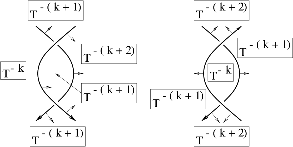
We define the twisted cocycle knot invariant in this section. First, we define the Alexander numbering for crossings.

Let $K$ be an oriented knot diagram with normals. Consider the underlying simple closed curve of $K$ , which is a generically immersed curve dividing the plane into regions, and let $R$ be one of the regions. Let $\alpha$ be an arc on the plane from a point in the region at infinity to a point $R$ such that the interior of $\alpha$ misses all the crossing points of $K$ and intersects transversely in finitely many points with the arcs of $K$ . A classically known concept called Alexander numbering (see for example [11, 7]) of $R$ , denoted by ${\cal L}(R)$ , is defined as the number, counted with signs, of the number of intersections between $\alpha$ and $K$ .

More specifically, when $\alpha$ is traced from the region at infinity to $R$ , and intersect at $p$ with $K$ , if the normal to $K$ at $p$ is the same direction as $\alpha$ , then $p$ contributes $+1$ to ${\cal L}(R)$ . If the direction of $\alpha$ is the opposite to the normal, then its contribution is $-1$ . The sum over all intersections does not depend on the choice of $\alpha$ .

In general, an Alexander numbering exists for an immersed curve in an orientable surface if and only if the curve represents a trivial $1$ -dimensional class in the homology of the surface.

Definition 7.1.

Let $K$ be an oriented knot diagram with normals. Let $\tau$ be a crossing. There are four regions near $\tau$ , and the unique region from which normals of over- and under-arcs point is called the source region of $\tau$ .

The Alexander numbering ${\cal L}(\tau)$ of a crossing $\tau$ is defined to be ${\cal L}(R)$ where $R$ is the source region of $\tau$ . Compare with [7].

In other words, ${\cal L}(\tau)$ is the number of intersections, counted with signs, between an arc $\alpha$ from the region at infinity to $\tau$ approaching from the source region of $\tau$ . In Fig. 2, the source region $R$ is the left-most region, and the Alexander numbering of $R$ is $k$ , and so is the Alexander numbering of the crossing $\tau$ .

Let a classical knot (or link) diagram $K$ , a finite quandle $X$ , a finite Alexander quandle $A$ be given. A coloring of $K$ by $X$ also is given and is denoted by ${\cal C}$ .

A twisted (Boltzmann) weight, $B_{T}(\tau,{\cal C})$ , at a crossing $\tau$ is defined as follows. Let ${\cal C}$ denote a coloring. Let $r$ be the over-arc at $\tau$ , and $r_{1}$ , $r_{2}$ be under-arcs such that the normal to $r$ points from $r_{1}$ to $r_{2}$ . Let $x={\cal C}(r_{1})$ and $y={\cal C}(r)$ . Pick a quandle 2-cocycle $\phi\in Z^{2}_{\rm TQ}(X;A)$ . Then define $B_{T}(\tau,{\cal C})=[\phi(x,y)^{\epsilon(\tau)}]^{T^{-{\cal L}(\tau)}}$ , where $\epsilon(\tau)=1$ or $-1$ , if the sign of $\tau$ is positive or negative, respectively. Here, we use the multiplicative notation of elements of $A$ , so that $\phi(x,y)^{-1}$ denotes the inverse of $\phi(x,y)$ . Recall that $A$ admits an action by $\mathbb{Z}=\{T^{n}\}$ , and for $a\in A$ , the action of $T$ on $a$ is denoted by $a^{T}$ . To specify the action by ${T^{-{\cal L}(\tau)}}$ in the figures, each region $R$ with Alexander numbering ${\cal L}(R)=k$ is labeled by the power $T^{-k}$ framed with a square, as depicted in Fig. 2.

The state-sum, or a partition function, is the expression

\Phi(K)=\sum_{{\cal C}}\prod_{\tau}B_{T}(\tau,{\cal C}).

The product is taken over all crossings of the given diagram, and the sum is taken over all possible colorings. The value of the weight $B_{T}(\tau,{\cal C})$ is in the coefficient group $A$ written multiplicatively. Hence the value of the state-sum is in the group ring ${\mathbb{Z}}[A]$ .

Theorem 7.2.

The state-sum is well-defined.

More specifically, let $\Phi(K_{1})$ and $\Phi(K_{2})$ be the state-sums obtained from two diagrams of the same knot, then we have $\Phi(K_{1})=\Phi(K_{2})$ .

Proof.

The invariance is proved by checking Reidemeister moves as follows. Since the $2$ -cocycle used satisfies $\phi(x,x)=1$ for any $x\in X$ , and the action of $T$ on the identity results in identity, the type I Reidemeister move does not alter the state-sum.

For the type II move, we note that the crossings involved in a type II move have opposite signs, and have the same Alexander numbering, see Fig. 3 for typical situations (other cases can be checked similarly). In both cases in the figure, all the crossings have the same Alexander numbering ${\cal L}(\tau)=k$ , as seen from the Alexander numberings of the adjacent regions specified in the figure by square-framed labels. Hence the contribution to the state-sum of the pair of crossings is of the form $[\phi(x,y)^{\epsilon}]^{T^{n}}[\phi(x,y)^{-\epsilon}]^{T^{n}}$ , which is trivial. Hence the state-sum is invariant under type II move.

Figure 4 depicts the situation for a type III move, for specific choices of crossing information and orientations. In this case, the left most crossings have the Alexander numbering $-1$ so that there is a $T$ -factor in the Boltzmann weight, and the right crossings, consequently, have numbering $0$ , and do not have the $T$ -factor. From the figure it is seen that the contributions to the state-sum, in this case, is exactly the $2$ -cocycle condition for the left and right hand side of the figure, and hence the state-sum remains unchanged. In the figure, the $T$ -action on cocycles is denoted in additive notation $T\phi(x,y)$ instead of multiplicative notation $\phi(x,y)^{T}$ , to match the $2$ -cocycle condition formulated in additive notation. The other cases follow from combinations with type II moves, see [21, 26] and [4] for more details. ∎

Example 7.3.

Let $X=T_{2}$ (the trivial two element quandle) and $A=$ $\mathbb{Z}[T,T^{-1}]/(T^{2}-1)$ . $\phi=T\chi_{0,1}+\chi_{1,0}$ is a cocycle in $Z^{2}_{\rm TQ}(X;A)$ . As an abelian group, $A$ is generated by $1$ and $T$ , each denoted multiplicatively by $s$ and $t$ , respectively. Thus any element of $A$ is written as $s^{m}t^{n}$ for integers $m,n$ , and the value of the invariant lies in $\mathbb{Z}[A]=\{a+bs^{m}t^{n}|a,b,m,n\in\mathbb{Z}\}$ .

A coloring of a Hopf link $L$ and computations of weights are depicted in Fig. 5. This specific contribution to the state-sum is $T+1$ , or $st$ . Note that both crossings have the Alexander numbering $-1$ , so the weight is multiplied by $T$ . By considering all possible colorings, we obtain $\Phi(L)=2+2st$ .

For knots and links on compact surfaces defined up to Reidemeister moves, a similar invariants can be defined. There are two modifications that have to be made.

(1) The regions divided by a given diagram have consistent colorings by powers of $T$ .

(2) Since there is no region at infinity, the choice of the “base” region must be considered.

Let $K$ be an oriented knot or link diagram on a compact oriented surface $F$ . Let $X$ be a finite quandle and $A$ be the coefficient group, which is a $\Lambda=\mathbb{Z}[T,T^{-1}]$ -module. Assume that $T^{n}=1$ for the action of $T$ on $A$ . Let $\phi\in Z^{2}_{\rm TQ}(X;A)$ .

Let $R_{i}$ , $i=0,1,\ldots,n$ , be the regions divided by $K$ , and call $R_{0}$ the base region. Define the mod $p$ Alexander numbering as before, except taking the values to be in $\mathbb{Z}_{p}$ , where $p$ is a positive integer.

If such a coloring of regions by $\mathbb{Z}_{p}$ is not possible, define $\Phi(K)=0$ . Otherwise, we proceed as follows. A coloring ${\cal C}$ of a knot diagram is defined similarly as before.

A twisted (Boltzmann) weight, $B_{T}(\tau,{\cal C})$ , at a crossing $\tau$ is defined similarly by $B_{T}(\tau,{\cal C})=[\phi(x,y)^{\epsilon(\tau)}]^{T^{-{\cal L}(\tau)}}$ . The state-sum, or a partition function, is defined similarly by $\Phi(K)=\sum_{{\cal C}}\prod_{\tau}B_{T}(\tau,{\cal C}).$

To state the theorem, we need the following convention. A typical element of ${\mathbb{Z}}[A]$ is of the form $\sum_{i=1}^{n}x_{i}a_{i}$ for a positive integer $n$ , where $x_{i}\in\mathbb{Z}$ and $a_{i}\in A$ . We define the action of $\mathbb{Z}=\langle T\rangle$ on ${\mathbb{Z}}[A]$ by $(\sum_{i=1}^{n}x_{i}a_{i})^{T}=\sum_{i=1}^{n}x_{i}(a_{i})^{T}$ . When a base region is replaced by another region, the state-sum changes by an action of $T^{k}$ for some integer $k$ . Thus a proof similar to the planar diagram case implies the following generalization.

Theorem 7.4.

The state-sum is well-defined up to the action of $\mathbb{Z}=\langle T\rangle$ for knots and links on surfaces.

More specifically, let $\Phi(K_{1})$ and $\Phi(K_{2})$ be the state-sums obtained from two diagrams of the same knot, then for some integer $k$ , we have $\Phi(K_{1})=\Phi(K_{2})^{T^{k}}$ .

Remark 7.5.

For planar link diagrams, one could “throw a string over the point at infinity,” to shift the Alexander numberings by $\pm 1$ . The same change can be realized by Reidemeister moves. This implies that the values of the invariant for planar link diagrams are polynomials invariant under $T$ -action.

Example 7.6.

A link $L$ on a torus is depicted in Fig. 6. A coloring by $X=R_{3}=\{a,b,c\}$ is given. Note that the action of $T$ on $A=R_{3}$ satisfies $T^{2}=1$ , so that a mod $2$ Alexander numbering is defined with $A=R_{3}$ . The base region is marked by $*$ . The base region has the Alexander numbering $0$ , and is labeled with the $T$ -term $T^{0}$ . The powers of $T$ that the other regions receive are depicted in the figure. Note that $T^{k+2}=T^{k}$ , so that regions are labeled by either $T^{0}$ or $T^{-1}=T$ . The left/right sides and top/bottom sides of the middle square have identical colorings and numberings, respectively. Thus these sides can be identified, as depicted, by bands, to obtain a punctured torus, and further the boundary can be capped off by a disk to obtain a torus. The contributions $\pm T^{j}\phi(x,y)$ to the Boltzmann weight of each crossing is indicated. For this specific coloring, the contribution is $\phi(a,b)-\phi(c,b)$ .

From Example 5.12 we have a $2$ -cocycle

\phi^{\prime}=2\chi_{0,1}+\chi_{0,2}+\chi_{1,0}+2\chi_{1,2}+2\chi_{2,0}+\chi_{2,1}\in Z^{2}_{\rm TQ}(R_{3};R_{3}).

With this cocycle, one computes that the invariant is $\Phi(L)=3+3t+3t^{2}$ . The action of $T$ on this element is $T\cdot(3+3t+3t^{2})=3+3t^{2}+3t$ so that the action does not change this element, and the class of the polynomial $3+3t+3t^{2}$ under $T$ -action consists of a single element.

It is seen that the invariant is trivial ( $=9$ ) if we use the cocycle $\phi$ in Example 5.4.

Proposition 7.7.

Let $X$ be a finite quandle, and let $A$ be an Alexander quandle. Suppose $\phi\in Z^{2}_{\rm TQ}(X;A)$ is a coboundary: $\phi=\delta\eta$ , where $\eta\in Z^{1}_{\rm TQ}(X;A)$ . Then the state-sum $\Phi(K)$ is a positive integer.

Proof.

By assumption we have

\phi(x_{1},x_{2})=\delta\eta(x_{1},x_{2})=-T\eta(x_{2})+T\eta(x_{1})+\eta(x_{2})-\eta(x_{1}*x_{2}).

For a given knot diagram $K$ , remove a small neighborhood of each crossing, and let $\gamma_{i}$ , $i=1,\ldots,m$ , be the resulting arcs. The end points of arcs are located near crossings, and depicted by dots in Fig. 7. Assign each term of the above right-hand side to the end points as depicted in the left crossing of Fig. 7. In the right of the figure, the situation at an adjacent crossing is also depicted. Note that the argument in $\eta$ coincides with the color (a quandle element) of the arc. Then it is seen that the terms assigned to the two end points of each arc are the same, with opposite signs (as is seen from Fig. 7). Hence the contribution to the state-sum for any coloring is $1$ , and the state-sum is a positive integer (which is the number of colorings). This argument is similar to the one given in [4]. ∎

Proposition 7.8.

Let $\phi\in Z^{2}_{\rm TQ}(X;N)$ be an obstruction $2$ -cocycle, where $X$ is a finite quandle and $N$ is an Alexander quandle. Then the state-sum invariant $\Phi(K)$ defined from $\phi$ is a positive integer for any link diagram $K$ on the plane.

Proof.

We have an exact sequence $0\rightarrow N\stackrel{{\scriptstyle i}}{{\rightarrow}}G\stackrel{{\scriptstyle p}}{{\rightarrow}}A\rightarrow 0$ of Alexander quandles, as in Theorem 4.14, and a section $s:A\rightarrow G$ with $ps=$ id, $s(0)=0$ . By Relation (7), for an obstruction cocycle $\phi$ , we have

i\phi(x_{1},x_{2})=Ts\eta(x_{1})+(1-T)s\eta(x_{2})-s\eta(x_{1}*x_{2}).

Using $s\eta(x)$ instead of $\eta$ in the proof of the preceding Proposition, we obtain the result. Here, the fact that $K$ is a planar diagram is used in the step claiming that $\pm T^{k}s\eta(x)$ assigned to endpoints of each arc cancel, since the $T$ -factor $T^{k}$ matches on both endpoints of each arc. More explanations on this point are in order. In the preceeding example of a link on a torus, the Alexander numbering of regions satisfy $T^{k}=T^{k+2}$ since $T^{2}=1$ as an action on $N=R_{3}$ , but the action of $T$ on the extension $AE(R_{3},R_{3},\phi)$ does not satisfy this relationship. Hence the terms $T^{k}s(x)$ and $-T^{k-2}s(x)$ assigned to endpoints of a single arc do not cancel in the extension. In other words, in the preceding theorem, the cancelation was made in the coefficient ring, but in this proof, the cancelations need to be done in the extension via sections and inclusions, and the Alexander numbering of the regions need to be consistent. The proof applies to such cases if the terms actually cancel, even if $K$ is non-planar. ∎

Example 7.9.

The link $L$ in Example 7.6 has a non-trivial state-sum invariant with the cocycle in Example 5.12, which was obtained from a short exact sequence of Alexander quandles. This is the case since, of course, $L$ is on a torus, and not on the plane.

Corollary 7.10.

Let $\phi\in Z^{2}_{\rm TQ}(X;A)$ be an obstruction $2$ -cocycle, where $X$ and $A$ are finite Alexander quandles. If the state-sum invariant $\Phi(K)$ defined from $\phi$ is non-trivial (i.e., not a positive integer) for a planar link diagram $K$ , then the Alexander extension $AE(X,A,\phi)$ is not an Alexander quandle such that

0{\rightarrow}A\stackrel{{\scriptstyle i}}{{\rightarrow}}A\times X=AE(X,A,\phi)\stackrel{{\scriptstyle p}}{{\rightarrow}}X\rightarrow 0

is a short exact sequence of $\Lambda$ -modules where $i$ and $p$ are the natural maps as in Remark 4.6.

Proof.

By Remark 4.6, if $AE(X,A,\phi)$ is an Alexander quandle, then a short exact sequence of Alexander quandles

0\rightarrow A\rightarrow A\times X=AE(X,A,\phi)\rightarrow X\rightarrow 0

defines an obstruction cocycle $\phi$ . This contradicts the preceding Theorem. ∎

Example 7.11.

The $2$ -cocycle $\phi$ $\in$ $Z^{2}_{\rm TQ}$ $(T_{2};$ $\mathbb{Z}[T,T^{-1}]/(T^{2}-1))$ used in Example 7.3 gave rise to a non-trivial value for a Hopf link. Hence $AE(T_{2},$ $\mathbb{Z}[T,T^{-1}]/(T^{2}-1),$ $\phi)$ is not an Alexander quandle of the form stated in the preceeding Corollary.

For $A=T_{2}$ , the cohomology theory is untwisted, and for $X=\mathbb{Z}_{2}[T,T^{-1}]/(T^{2}+T+1)$ , it is known [5] that $\phi=\sum_{a\neq b,a\neq T\neq b}\chi_{a,b}$ is a cocycle. With this cocycle, there are a number of classical knots in the table with non-trivial invariant. Hence $AE(\mathbb{Z}_{2}[T,T^{-1}]/(T^{2}+T+1),T_{2},\phi)$ is not an Alexander quandle of the form stated in the preceeding Corollary.

The state-sum invariant is defined in an analogous way for oriented knotted surfaces in $4$ -space using their projections and diagrams in $3$ -space. Specifically, the above steps can be repeated as follows, for a fixed finite quandle $X$ and a knotted surface diagram $K$ .

•

The diagrams consist of double curves and isolated branch and triple points [11]. Along the double curves, the coloring rule is defined using normals in the same way as classical case, as depicted in the left of Fig. 8.
•

The source region $R$ and the Alexander numbering ${\cal L}(\tau)={\cal L}(R)$ are defined for a triple point $\tau$ using normals.
•

A $3$ -cocycle $\theta\in Z^{3}_{\rm TQ}(X;A)$ , with the Alexander quandle coefficient $A$ is fixed, and assigned to a triple point as depicted in the right of Fig. 8. In this figure, the triple point has the Alexander numbering $0$ .
•

The sign $\epsilon(\tau)$ of a triple point $\tau$ is defined [11].
•

For a coloring ${\cal C}$ , the Boltzmann weight at a triple point $\tau$ is defined by

$B_{T}(\tau,{\cal C})=[\theta(x,y,z)^{\epsilon(\tau)}]^{T^{-{\cal L}(\tau)}}$ .
•

The state-sum is defined by $\sum_{{\cal C}}\prod_{\tau}B_{T}(\tau,{\cal C}).$

By checking the analogues of Reidemeister moves for knotted surface diagrams, called Roseman moves, we obtain the following.

Theorem 7.12.

The state-sum is well-defined for knotted surfaces, and is called the twisted quandle cocycle invariant of knotted surfaces.

Example 7.13.

Let $X=T_{3}=\{0,1,2\}$ (the trivial three element quandle) and $A=\mathbb{Z}[T,T^{-1}]/(T^{2}-1)$ . Recall that $\partial=(T-1)\partial_{0}$ as seen in Example 3.3, and $(T+1)(T-1)=0$ in $A$ . It follows that $\theta=(T+1)\chi_{0,1,2}$ is a cocycle in $Z^{3}_{\rm TQ}(X;A)$ (in fact, this construction works in Example 7.3 as well). Denote the multiplicative generators of $A$ by $s$ and $t$ , for additive generators $1$ and $T$ , respectively.

In Fig. 9, an analogue of a Hopf link for surfaces in $4$ -space, $L=K_{1}\cup K_{2}\cup K_{3}$ , is depicted. Each component is standardly embedded in $4$ -space, $K_{1}\cup K_{2}$ is the spun Hopf link with each component torus, and $K_{3}$ is a sphere (in the figure, a large “window” is cut out from $K_{3}$ to show an inside view). The top horizontal sheet of $K_{3}$ is the bottom sheet for the triple points $\tau_{1}$ and $\tau_{2}$ (that are positive triple points), and the bottom horizontal sheet of $K_{3}$ is the top sheet for $\tau_{3}$ and $\tau_{4}$ (that are negative triple points). The orientation normals all point inside, so that all the triple points are negative, using the right-hand convention of the orientation of the $3$ -space. The source region is the region at infinity for all triple points, so that the $T$ -factor coming from the Alexander numbering is $T^{0}=1$ for all the triple points.

The colors of relevant sheets are denoted by $x$ , $y$ , $z$ , for sheets in $K_{3}$ , $K_{2}$ , and $K_{1}$ , respectively, as depicted. When trivial quandles are used, the colors depend only on the components. Hence the state-sum term is written by

\theta(x,y,z)\theta(x,z,y)\theta(y,z,x)^{-1}\theta(z,y,x)^{-1}

where each term of $\theta$ coming from triple points $\tau_{i}$ , $i=1,2,3,4$ , respectively.

If the colors are given by $(x,y,z)=(0,1,2)$ , $\theta(x,y,z)=T+1$ additively and $st$ multiplicatively, for example, and the above state-sum term is equal to $st$ , since all the other $\theta$ terms are trivial. The coloring $(x,y,z)=(0,2,1)$ also contributes $st$ . The colorings $(x,y,z)=(2,0,1),(2,1,0)$ contributes $(st)^{-1}$ . All the other colorings contribute $1$ , and the invariant is $\Phi(L)=23+2st+2(st)^{-1}$ .

In fact, as in the classical case, the state-sum invariant is defined modulo the action by $T$ for knotted surface diagrams in compact orientable $3$ -manifolds, up to Roseman moves. Such diagrams up to Roseman moves can be regarded as ambient isotopy classes of embeddings of surfaces in the product space $M\times[0,1]$ , where $M$ is a compact orientable $3$ -manifold.

A similar argument to the proof of Proposition 7.7 gives the following analogue, see Fig. 10. In this figure, a negative triple point is depicted, so that the terms are the negative of those that appear in $\delta\theta$ . There is a diagram without branch point for orientable knotted surfaces (see for example [10]), so that the terms assigned to the end points of double arcs cancel as in classical case, and we obtain the following.

Proposition 7.14.

Let $X$ be a finite quandle, and let $A$ be an Alexander quandle. Suppose $\theta\in Z^{3}_{\rm TQ}(X;A)$ is a coboundary: $\theta=\delta\phi$ , where $\phi\in Z^{2}_{\rm TQ}(X;A)$ . Then the state-sum $\Phi(K)$ for a knotted surface is a positive integer.

A similar argument to the proof of Proposition 7.14 and that of Theorem 7.8 can be applied to obtain the following.

Proposition 7.15.

Let $\theta\in Z^{3}_{\rm TQ}(X;N)$ be an obstruction $3$ -cocycle, where $X$ is a finite quandle and $A$ is an Alexander quandle. Then the state-sum invariant $\Phi(K)$ defined from $\theta$ is a positive integer for any knotted surface diagram $K$ in Euclidean $3$ -space ${\mathbb{R}}^{3}$ .

Corollary 7.16.

Let $\theta\in Z^{3}_{\rm TQ}(X;N)$ an obstruction $3$ -cocycle, where $X$ and $A$ are finite Alexander quandles. If the state-sum invariant $\Phi(K)$ defined from $\theta$ is non-trivial (i.e., not a positive integer) for a knotted surface diagram $K$ in ${\mathbb{R}}^{3}$ , then $\theta$ is not an obstruction cocycle.

Example 7.17.

By the preceding Corollary and Example 7.13, we find that the cocycle in Example 7.13 is not an obstruction cocycle.

Remark 7.18.

As another application of colored knot diagrams, we exhibit a diagrammatic construction of the proof of Lemma 4.11. Diagrammatic methods in cohomology theory, such as Hochschild cohomology, are found, for example, in [22].

In the state-sum invariant, a $3$ -cocycle is assigned to a triple point as a Boltzmann weight. When a height function in $3$ -space is chosen, a triple point is described by the Reidemeister type III move. Cross sections of three sheets at a triple point by planes normal to the chosen height function give rise to a move among three strings, and the move is exactly the type III move. See [11] for more details. In Fig. 11, the type III move as such a movie description of a colored triple point is depicted. In this movie, we color the diagrams by quandle elements, assign $2$ -cocycles to crossings, assign $3$ -cocycles to type III move performed, and the convention of these assignments is depicted in Fig. 11.

In Figs. 12 and 13, diagrams involving four strings are depicted. These are cross sections of three coordinate planes in $3$ -space plus another plane in general position with the coordinate planes. See [11] for more details. The colorings by quandle elements and $2$ -cocycles are also depicted. Note that the $2$ -cocycles depicted in Fig. 12 are exactly the first expression of in the proof of Lemma 4.11, and those in Fig. 13 are the last expression, respectively.

There are two distinct sequences of type III moves that change Fig. 12 to Fig. 13. Each type III move gives rise to a $3$ -cocycle via the convention established in Fig. 11. It is seen that the two sequences of $3$ -cocycles corresponding to two sequences of type III moves are identical to the sequences of equalities in the proof of Lemma 4.11. Once the direct correspondence is made, the computations follows from these diagrams automatically.

References

[1] E Brieskorn, Automorphic sets and singularities, Contemporary Math., 78 (1988) 45–115.
[2] K H Brown, Cohomology of groups, Graduate Texts in Mathematics, 87. Springer-Verlag, New York-Berlin (1982).
[3] J S Carter, M Elhamdadi, M A Nikiforou, M Saito, Extensions of quandles and cocycle knot invariants, preprint, arxiv:math.GT/0107021
[4] J S Carter, D Jelsovsky, S Kamada, L Langford, M Saito, Quandle cohomology and state-sum invariants of knotted curves and surfaces, to appear Trans AMS, preprint, arxiv:math.GT/9903135
[5] J S Carter, D Jelsovsky, S Kamada, M Saito, Computations of quandle cocycle invariants of knotted curves and surfaces, Advances in Math., 157 (2001) 36–94.
[6] J S Carter, D Jelsovsky, S Kamada, M Saito, Quandle homology groups, their betti numbers, and virtual knots, J. of Pure and Applied Algebra, 157, (2001), 135–155.
[7] J S Carter, S Kamada, M Saito, Alexander numbering of knotted surface diagrams, Proc. A.M.S. 128 no 12 (2000) 3761–3771.
[8] J S Carter, S Kamada, M Saito, Geometric interpretations of quandle homology, J. of Knot Theory and its Ramifications, 10, no. 3 (2001) 345–386.
[9] J S Carter, S Kamada, M Saito, Diagrammatic Computations for Quandles and Cocycle Knot Invariants, preprint, arxiv:math.GT/0102092
[10] J S Carter, M Saito, Canceling branch points on the projections of surfaces in 4-space, Proc. A. M. S. 116, 1, (1992) 229–237.
[11] J S Carter, M Saito, Knotted surfaces and their diagrams, the American Mathematical Society, (1998).
[12] V G Drinfeld, Quantum groups, Proceedings of the International Congress of Mathematicians, Vol. 1, 2 (Berkeley, Calif., 1986) 798–820, Amer. Math. Soc., Providence, RI, 1987.
[13] R Fenn, C Rourke, Racks and links in codimension two, Journal of Knot Theory and Its Ramifications Vol. 1 No. 4 (1992) 343–406.
[14] R Fenn, C Rourke, B J Sanderson, Trunks and classifying spaces, Appl. Categ. Structures 3 no 4 (1995) 321–356.
[15] R Fenn, C Rourke, B J Sanderson, James bundles and applications, preprint found at http://www.maths.warwick.ac.uk/^∼cpr/ftp/james.ps
[16] J Flower, Cyclic Bordism and Rack Spaces, Ph.D. Dissertation, Warwick (1995).
[17] R H Fox, A quick trip through knot theory, in Topology of $3$ -Manifolds, Ed. M.K. Fort Jr., Prentice-Hall (1962) 120–167.
[18] M Gerstenhaber, S D Schack, Bialgebra cohomology, deformations, and quantum groups. Proc. Nat. Acad. Sci. U.S.A. 87 no. 1 (1990) 478–481.
[19] M T Greene, Some Results in Geometric Topology and Geometry, Ph.D. Dissertation, Warwick (1997).
[20] D Joyce, A classifying invariant of knots, the knot quandle, J. Pure Appl. Alg., 23, 37–65.
[21] L H Kauffman, Knots and Physics, World Scientific, Series on knots and everything, vol. 1, 1991.
[22] M Markl, J D Stasheff, Deformation theory via deviations. J. Algebra 170 no. 1 (1994) 122–155.
[23] S Matveev, Distributive groupoids in knot theory, (Russian) Mat. Sb. (N.S.) 119(161) no. 1 (1982) 78–88, 160.
[24] D Rolfsen, Knots and Links, Publish or Perish Press, (Berkeley 1976).
[25] C Rourke, B J Sanderson, There are two $2$ -twist-spun trefoils, preprint, arxiv:math.GT/0006062
[26] V Turaev, The Yang-Baxter equation and invariants of links, Invent. Math. 92 (1988) 527–553.
[27] E C Zeeman, Twisting spun knots, Trans. Amer. Math. Soc. 115 (1965) 471–495.

\Addresses

Received:\qua27 September 2001

$\displaystyle[(a_{1},x_{1})(a_{2},x_{2})](a_{3},x_{3})$
	$\displaystyle=$	$\displaystyle(Ta_{1}+(1-T)a_{2}+\phi(x_{1},x_{2}),x_{1}x_{2})(a_{3},x_{3})$
	$\displaystyle=$	$\displaystyle(T[Ta_{1}+(1-T)a_{2}+\phi(x_{1},x_{2})]$
		$\displaystyle+(1-T)a_{3}+\phi(x_{1}x_{2},x_{3}),(x_{1}x_{2})*x_{3})$
	$\displaystyle=$	$\displaystyle((a_{1}a_{2})a_{3}+T\phi(x_{1},x_{2})$
		$\displaystyle+\phi(x_{1}x_{2},x_{3}),(x_{1}x_{2})*x_{3}),$

$\displaystyle[(a_{1},x_{1})(a_{3},x_{3})][(a_{2},x_{2})*(a_{3},x_{3})]$
	$\displaystyle=$	$\displaystyle(a_{1}a_{3}+\phi(x_{1},x_{3}),x_{1}x_{3})(a_{2}a_{3}+\phi(x_{2},x_{3}),x_{2}*x_{3})$
	$\displaystyle=$	$\displaystyle(T[a_{1}a_{3}+\phi(x_{1},x_{3})]+(1-T)[a_{2}a_{3}+\phi(x_{2},x_{3})]$
		$\displaystyle+\phi(x_{1}x_{3},x_{2}x_{3}),(x_{1}x_{3})(x_{2}*x_{3}))$
	$\displaystyle=$	$\displaystyle((a_{1}a_{3})(a_{2}*a_{3})+T\phi(x_{1},x_{3})+(1-T)\phi(x_{2},x_{3})$
		$\displaystyle+\phi(x_{1}x_{3},x_{2}x_{3}),(x_{1}x_{3})(x_{2}*x_{3})).$

		$\displaystyle=$	$\displaystyle[iT\theta(x_{1},x_{2},x_{3})+i\theta(x_{1}x_{3},x_{2}x_{3},x_{4})]$
			$\displaystyle+[\underline{s\phi(x_{2}x_{3},x_{4})+Ts\phi(x_{1}x_{3},x_{4})}$
			$\displaystyle+s\phi((x_{1}x_{3})x_{4},(x_{2}x_{3})x_{4})]$
			$\displaystyle+\underline{T^{2}s\phi(x_{1},x_{3})}+Ts\phi(x_{2},x_{3})+\underline{T^{2}s\phi(x_{3},x_{4})}$
		$\displaystyle=$	$\displaystyle[iT\theta(x_{1},x_{2},x_{3})+i\theta(x_{1}x_{3},x_{2}x_{3},x_{4})+iT\theta(x_{1},x_{3},x_{4})]$
			$\displaystyle+[\underline{Ts\phi(x_{3},x_{4})}+T^{2}s\phi(x_{1},x_{4})+Ts\phi(x_{1}x_{4},x_{3}x_{4})]$
			$\displaystyle+s\phi((x_{1}x_{3})x_{4},(x_{2}x_{3})x_{4})+\underline{Ts\phi(x_{2},x_{3})+s\phi(x_{2}*x_{3},x_{4})}$
		$\displaystyle=$	$\displaystyle[iT\theta(x_{1},x_{2},x_{3})+i\theta(x_{1}x_{3},x_{2}x_{3},x_{4})$
			$\displaystyle+iT\theta(x_{1},x_{3},x_{4})+i\theta(x_{2},x_{3},x_{4})]$
			$\displaystyle+[s\phi(x_{3},x_{4})+Ts\phi(x_{2},x_{4})+s\phi(x_{2}x_{4},x_{3}x_{4})]$
			$\displaystyle+T^{2}s\phi(x_{1},x_{4})+Ts\phi(x_{1}x_{4},x_{3}x_{4})$
			$\displaystyle+s\phi((x_{1}x_{3})x_{4},(x_{2}x_{3})x_{4})$

$\displaystyle T^{2}s\phi(x_{1},x_{2})+Ts\phi(x_{1}*x_{2},x_{3})+\underline{T^{2}s\phi(x_{2},x_{3})}$
		$\displaystyle+s\phi((x_{1}x_{2})x_{3},x_{4})+\underline{Ts\phi(x_{2}*x_{3},x_{4})+T^{2}s\phi(x_{3},x_{4})}$
	$\displaystyle=$	$\displaystyle iT\theta(x_{2},x_{3},x_{4})+[\underline{Ts\phi(x_{3},x_{4})}+T^{2}s\phi(x_{2},x_{4})+Ts\phi(x_{2}x_{4},x_{3}x_{4})]$
		$\displaystyle+T^{2}s\phi(x_{1},x_{2})+\underline{Ts\phi(x_{1}x_{2},x_{3})+s\phi((x_{1}x_{2})*x_{3},x_{4})}$
	$\displaystyle=$	$\displaystyle[iT\theta(x_{2},x_{3},x_{4})+i\theta(x_{1}*x_{2},x_{3},x_{4})]$
		$\displaystyle+[s\phi(x_{3},x_{4})+\underline{Ts\phi(x_{1}x_{2},x_{4})}+s\phi((x_{1}x_{2})x_{4},x_{3}x_{4})]$
		$\displaystyle+\underline{T^{2}s\phi(x_{2},x_{4})}+Ts\phi(x_{2}x_{4},x_{3}x_{4})+\underline{T^{2}s\phi(x_{1},x_{2})}$
	$\displaystyle=$	$\displaystyle[iT\theta(x_{2},x_{3},x_{4})+i\theta(x_{1}*x_{2},x_{3},x_{4})+iT\theta(x_{1},x_{2},x_{4})]$
		$\displaystyle+[Ts\phi(x_{2},x_{4})+T^{2}s\phi(x_{1},x_{4})+\underline{Ts\phi(x_{1}x_{4},x_{2}x_{4})}]$
		$\displaystyle+\underline{s\phi((x_{1}x_{2})x_{4},x_{3}x_{4})}+\underline{Ts\phi(x_{2}x_{4},x_{3}*x_{4})}+s\phi(x_{3},x_{4})$
	$\displaystyle=$	$\displaystyle[iT\theta(x_{2},x_{3},x_{4})+i\theta(x_{1}*x_{2},x_{3},x_{4})$
		$\displaystyle+iT\theta(x_{1},x_{2},x_{4})+i\theta(x_{1}x_{4},x_{2}x_{4},x_{3}*x_{4})]$
		$\displaystyle+[s\phi(x_{2}x_{4},x_{3}x_{4})+Ts\phi(x_{1}x_{4},x_{3}x_{4})$
		$\displaystyle+s\phi((x_{1}x_{3})x_{4},(x_{2}x_{3})x_{4})]$
		$\displaystyle+T^{2}s\phi(x_{1},x_{4})+Ts\phi(x_{2},x_{4})+s\phi(x_{3},x_{4})$

$\displaystyle[(a_{1},x_{1})(a_{2},x_{2})](a_{3},x_{3})$
	$\displaystyle=$	$\displaystyle(a_{1}a_{2}+\phi(x_{1},x_{2}),x_{1}x_{2})*(a_{3},x_{3})$
	$\displaystyle=$	$\displaystyle((a_{1}a_{2})a_{3}+T\phi(x_{1},x_{2})+\phi(x_{1}x_{2},x_{3}),(x_{1}x_{2})*x_{3}),$

Twisted quandle homology theoryand cocycle knot invariants

Abstract

keywords

1 Introduction

2 Quandles and their homology theory

3 Twisted quandle homology

Example 3.1.

Example 3.2.

Example 3.3.

Proposition 3.4.

Example 3.5.

4 Extensions of quandles by Alexander quandles

Lemma 4.1.

Proof.

Lemma 4.2.

Proof.

Lemma 4.3.

Proof.

Theorem 4.4.

Lemma 4.5.

Proof.

Remark 4.6.

Definition 4.7.

Lemma 4.8.

Proof.

Lemma 4.9.

Proof.

Theorem 4.10.

Lemma 4.11.

Proof.

Lemma 4.12.

Proof.

Lemma 4.13.

Proof.

Theorem 4.14.

5 Alexander quandles as Alexander extensions

Lemma 5.1.

Proof.

Lemma 5.2.

Proof.

Corollary 5.3.

Example 5.4.

Proposition 5.5.

Proof.

Example 5.6.

Proposition 5.7.

Proof.

Theorem 5.8.

Proof.

Corollary 5.9.

Lemma 5.10.

Proof.

Theorem 5.11.

Proof.

Example 5.12.

Proposition 5.13.

Proof.

Remark 5.14.

6 Cohomology with H1H^{1} coefficients

Proposition 6.1.

Proof.

Example 6.2.

Example 6.3.

Proposition 6.4.

Proof.

7 Twisted cocycle knot invariants

Definition 7.1.

Theorem 7.2.

Proof.

Example 7.3.

Theorem 7.4.

Remark 7.5.

Example 7.6.

Proposition 7.7.

Proof.

Proposition 7.8.

Proof.

Example 7.9.

Corollary 7.10.

Proof.

6 Cohomology with $H^{1}$ coefficients