Topological Deformation of Higher Dimensional Automata

Philippe Gaucher Affiliation: Institut de Recherche Mathématique Avancée, ULP et CNRS,7 rue René Descartes, 67084 Strasbourg Cedex Eric Goubault Affiliation: LIST (CEA - Recherche Technologique)DTSI-SLA, CEA F91191 Gif-sur-Yvette Cedex

July 2002

Abstract

A local po-space is a gluing of topological spaces which are equipped with a closed partial ordering representing the time flow. They are used as a formalization of higher dimensional automata (see for instance [6]) which model concurrent systems in computer science. It is known [11] that there are two distinct notions of deformation of higher dimensional automata, “spatial” and “temporal”, leaving invariant computer scientific properties like presence or absence of deadlocks. Unfortunately, the formalization of these notions is still unknown in the general case of local po-spaces.

We introduce here a particular kind of local po-space, the “globular CW-complexes”, for which we formalize these notions of deformations and which are sufficient to formalize higher dimensional automata. The existence of the category of globular CW-complexes was already conjectured in [11].

After localizing the category of globular CW-complexes by spatial and temporal deformations, we get a category (the category of dihomotopy types) whose objects up to isomorphism represent exactly the higher dimensional automata up to deformation. Thus globular CW-complexes provide a rigorous mathematical foundation to study from an algebraic topology point of view higher dimensional automata and concurrent computations.

1 Introduction

Algebraic topological models have been used now for some years in concurrency theory (concurrent database systems and fault-tolerant distributed systems as well). The earlier models, progress graph (see [3] for instance) have actually appeared in operating systems theory, in particular for describing the problem of ‘‘deadly embrace’’¹¹ 1 as E. W. Dijkstra originally put it in [4], now more usually called deadlock. in “multiprogramming systems”.

The basic idea is to give a description of what can happen when several processes are modifying shared resources. Given a shared resource $a$ , we see it as its associated semaphore that rules its behaviour with respect to processes. For instance, if $a$ is an ordinary shared variable, it is customary to use its semaphore to ensure that only one process at a time can write on it (this is mutual exclusion). A semaphore is nothing but a register which counts the number of times a shared object can still be accessed by processes. In the case of usual shared variables, this register is initialized with value 1, processes trying to access (read or write) on the corresponding variable compete in order to get it first, then the semaphore value is decreased: we say that the semaphore has been locked²² 2 Of course this operation must be done “atomically”, meaning that the semaphore itself must be handled in a mutually exclusive manner: this is done at the hardware level. by the process. When it is equal to zero, all processes trying to access this semaphore are blocked, waiting for the process which holds the lock to relinquish it, typically when it has finished reading or writing on the corresponding variable: the value of the semaphore is then increased.

When the semaphores are initialized with value one, meaning that they are associated with shared variables accessed in a mutually exclusive manner, they are called binary semaphores. When a shared data (identified with its semaphore) can be accessed by one or more processes, meaning that the corresponding semaphore has been initialized with a value greater than one, it is called a counting semaphore.

Given $n$ deterministic sequential processes $Q_{1},\ldots,Q_{n}$ , abstracted as a sequence of locks and unlocks on (semaphores associated with) shared objects, $Q_{i}=R^{1}a_{i}^{1}.R^{2}a_{i}^{2}\cdots R^{n_{i}}a_{i}^{n_{i}}$ ( $R^{k}$ being $P$ or $V$ ³³ 3 Using E. W. Dijkstra’s notation $P$ and $V$ [4] for respectively acquiring and releasing a lock on a semaphore.), there is a natural way to understand the possible behaviours of their concurrent execution, by associating to each process a coordinate line in $\mathbb{R}^{n}$ . The state of the system corresponds to a point in $\mathbb{R}^{n}$ , whose $i$ th coordinate describes the state (or “local time”) of the $i$ th processor.

Consider a system with finitely many processes running altogether. We assume that each process starts at (local time) 0 and finishes at (local time) 1; the $P$ and $V$ actions correspond to sequences of real numbers between 0 and 1, which reflect the order of the $P$ ’s and $V$ ’s. The initial state is $(0,\dots,0)$ and the final state is $(1,\dots,1)$ . An example consisting of the two processes $T_{1}=Pa.Pb.Vb.Va$ and $T_{2}=Pb.Pa.Va.Vb$ gives rise to the two dimensional progress graph of Figure 1.

Refer to caption — Figure 1: Example of a progress graph

The shaded area represents states which are not allowed in any execution path, since they correspond to mutual exclusion. Such states constitute the forbidden area. An execution path is a path from the initial state $(0,\ldots,0)$ to the final state $(1,\ldots,1)$ avoiding the forbidden area and increasing in each coordinate - time cannot run backwards. We call these paths directed paths or dipaths. This entails that paths reaching the states in the dashed square underneath the forbidden region, marked “unsafe” are deemed to deadlock, i.e. they cannot possibly reach the allowed terminal state which is $(1,1)$ here. Similarly, by reversing the direction of time, the states in the square above the forbidden region, marked “unreachable”, cannot be reached from the initial state, which is $(0,0)$ here. Also notice that all terminating paths above the forbidden region are “equivalent” in some sense, given that they are all characterized by the fact that $T_{2}$ gets $a$ and $b$ before $T_{1}$ (as far as resources are concerned, we call this a schedule). Similarly, all paths below the forbidden region are characterized by the fact that $T_{1}$ gets $a$ and $b$ before $T_{2}$ does.

On this picture, one can already recognize many ingredients that are at the center of the main problem of algebraic topology, namely the classification of shapes modulo “elastic deformation”. As a matter of fact, the actual coordinates that are chosen for representing the times at which $P$ s and $V$ s occur are unimportant, and these can be “stretched” in any manner, so the properties (deadlocks, schedules etc.) are invariant under some notion of deformation, or homotopy. This is only a particular kind of homotopy though, and this explains why a new theory has to be designed. We call it (in subsequent work) directed homotopy or dihomotopy in the sense that it should preserve the direction of time. For instance, the two homotopic shapes, all of which have two holes, of Figure 2 and Figure 3 have a different number of dihomotopy classes of dipaths. In Figure 2 there are essentially four dipaths up to dihomotopy (i.e. four schedules corresponding to all possibilities of accesses of resources $a$ and $b$ ) whereas in Figure 3, there are essentially three dipaths up to dihomotopy.

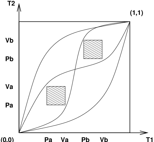
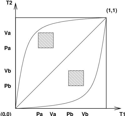
Progress graphs have actually a nice topological model; they are compact order-Hausdorff spaces (see [26], [21]), i.e. are compact Hausdorff spaces with a closed (global) partial order. More general topological models are needed in general, in which the partial order is only defined locally, and have been introduced and motivated in [7], [5] and [6]. The precise definitions and properties are given in Section 3.1.

The natural combinatorial notion which discretizes this topological framework is that of a precubical set, which is a collection of points (states), edges (transitions), squares, cubes and hypercubes (higher-dimensional transitions representing the truly-concurrent execution of some number of actions). This is introduced in [27] as well as possible formalizations using $n$ -categories, and a notion of homotopy. These precubical sets are called Higher-Dimensional Automata (HDA) following [27] because it really makes sense to consider a hypercube as some form of transition (as in transition systems, used in semantics of programming languages). We show the precise relation between this model and the new topological model we introduce here (“globular CW-complexes”) in Section 3.2, the relation between local po-spaces and cubical sets can be found in [6].

There are other formulations of the same problems using homological methods [15], strict globular $\omega$ -categories [12]. An important motivation in these pieces of work is that of “reducing the complexity” of the semantics (given by a local po-space for instance) by considering deformation retracts. The classification of the possible concurrent semantics (and behaviours) should then be the result finding the right “(di-)homotopy types”. This calls for a suitable notion of (di-)homotopy equivalence, and for starting with a reasonable category of local po-spaces. In the case of ordinary homotopy theory, we have to restrict to the category of CW-complexes; the category of topological spaces being far too big for practical purposes. The situation is even worse here, we not only have to restrict on the topology part, but also on the local po-structures.

We give in this paper a notion of CW-complex, called globular CW-complex which meets the basic requirements of what we expect to be a “directed cellular complex”. It has been obtained by mimicking the well-known concept of CW-complexes, but built from “directed” cells. This is the purpose of Section 2. Still in the same section, we introduce the fundamental functor called the globe functor, from the category of topological spaces to the category of po-spaces. This functor is the key to understanding how things work in the directed situation. In particular, it yields an embedding of the category of homotopy types into the new category of dihomotopy types (Theorem 5.9). This embedding has a lot of important consequences that are sketched in the perspectives section of [13].

Once the right notion has been given, we make explicit the link between the globular CW-complexes and some geometric notions above mentioned, that is the local po-spaces and the precubical sets in Section 3. We prove that every globular CW-complex is a local po-space indeed (Theorem 3.3) and that there exists a geometric realization of any precubical set as a globular CW-complex (subsection 3.3).

Next in Section 4 we recast in the globular CW-complex framework the notion of spatial and temporal deformations informally presented in [11] and whose consequences are informally explored in [13]. For that we construct, by localization of the category of globular CW-complexes with respect to appropriate morphisms, three categories whose isomorphism classes of objects are exactly the globular CW-complexes modulo spatial deformations (Theorem 4.7), the globular CW-complexes modulo temporal deformations (Theorem 4.12) and at last the globular CW-complexes modulo spatial and temporal deformations together (Theorem 4.16). This latter category will be called the category of dihomotopy types.

Then Section 5 is devoted to making explicit the link between homotopy types and dihomotopy types. The introduction of the path space of a globular CW-complex between two points of its $0$ -skeleton is the essential ingredient in the proof of Theorem 5.7 and Corollary 5.8. This allows us to derive the embedding theorem Theorem 5.9 which states that there exists an embedding of the category of homotopy types into that of dihomotopy types. This notion of path spaces also allows us to provide a conjectural statement for the analogue of the Whitehead theorem in the directed framework, and to check it in the case of globes.

Section 6 focuses on a very striking reason why it is necessary to work with “non-contracting” maps everywhere. It was not really possible to justify this axiom while the definition of globular CW-complexes was being given in Section 2. Only one reason is described. Indeed there are lots of other algebraic reasons which are out of the scope of this paper.

2 Globular CW-complexes

This section is devoted to the introduction of the category ${\rm{\mathbf{glCW}}}$ of globular CW-complexes and to the comparison with the usual notion of CW-complex.

2.1 Closed partial order

Definition 2.1.

Let $X$ be a topological space. A binary relation $R$ on $X$ is closed if the graph of $R$ is a closed subset of the cartesian product $X\times X$ .

It is a well-known fact that any topological space $X$ endowed with a closed partial order is necessarily Hausdorff (see for instance [26], [21]).

Definition 2.2.

A pair $(X,\leqslant_{X})$ where $X$ is a topological space and $\leqslant_{X}$ a closed partial order is called a global po-space.

In most cases, the partial order of a global po-space $X$ will be simply denoted by $\leqslant$ . Here are two fundamental examples of global po-spaces for the sequel :

1.

The achronal segment $\mathbb{I}$ is defined to be the segment $[0,1]$ endowed with the closed partial ordering $x\leqslant_{\mathbb{I}}y$ if and only if $x=y$ .
2.

The directed segment $\overrightarrow{I}$ is defined to be the segment $[0,1]$ endowed with the closed partial ordering $x\leqslant_{\overrightarrow{I}}y$ if and only if $y-x$ is non-negative.

We will describe gluings of global po-spaces (i.e. local po-spaces) in Section 3.1.

2.2 The globe of a topological space

Let $n\geqslant 1$ . Let $D^{n}$ be the closed $n$ -dimensional disk defined by the set of points $(x_{1},\dots,x_{n})$ of $\mathbb{R}^{n}$ such that $x_{1}^{2}+\dots+x_{n}^{2}\leqslant 1$ endowed with the topology induced by that of $\mathbb{R}^{n}$ . Let $S^{n-1}=\partial D^{n}$ be the boundary of $D^{n}$ for $n\geqslant 1$ , that is the set of $(x_{1},\dots,x_{n})\in D^{n}$ such that $x_{1}^{2}+\dots+x_{n}^{2}=1$ . Notice that $S^{0}$ is the discrete two-point topological space $\{-1,+1\}$ . Let $D^{0}$ be the one-point topological space. And let $e^{n}:=D^{n}-S^{n}$ .

The fundamental ingredient in all further constructions is the globe functor (Figure 4) defined below, which will give rise to a particular family of global po-spaces. Loosely speaking the globe of a topological space $X$ is the reduced suspension of $X$ equipped with some closed partial ordering representing the time flow.

The underlying topological space of the globe of a topological space $X$ , $Glob(X)$ , is therefore the quotient of the product space $X\times[0,1]$ by the relations $(x,0)=(x^{\prime},0)$ and $(x,1)=(x^{\prime},1)$ for any $x,x^{\prime}\in X$ . By convention, the equivalence class of $(x,0)$ (resp. $(x,1)$ ) in $Glob(X)$ will be denoted by $\underline{\iota}$ (resp. $\underline{\sigma}$ ). We can partially order $Glob(X)$ using the standard order $\leqslant_{I}$ on $I=[0,1]$ as follows :

Proposition 2.3.

Let $X$ be a Hausdorff topological space and consider the partial ordering of $X\times I$ defined by $\mathcal{R}=\{((x,t),(x,t^{\prime})),(x,t,t^{\prime})\in X\times I\times I\hbox{ and }t\leqslant_{I}t^{\prime}\}$ . Then its image by the canonical surjection $s$ from $X\times I$ to $Glob(X)$ is a closed partial ordering on $Glob(X)$ .

The partial order relation on $Glob(X)$ is as follows:

•

$(x,0)\leqslant(x^{\prime},t^{\prime})$ for all $x,x^{\prime},t^{\prime}\in X\times X\times I$ ,
•

when $t,t^{\prime}\in]0,1[\times]0,1[$ , $(x,t)\leqslant(x^{\prime},t^{\prime})$ if and only if $x=x^{\prime}$ ,
•

$(x^{\prime},t^{\prime})\leqslant(x,1)$ for all $x,x^{\prime},t^{\prime}\in X\times X\times I$ .

Proof.

By the homeomorphism $(x,t,x^{\prime},t^{\prime})\mapsto(x,x^{\prime},t,t^{\prime})$ from $X\times I\times X\times I$ to $X\times X\times I\times I$ , one sees that $\mathcal{R}$ is a closed subset of $X\times I\times X\times I$ if and only if $Diag(X)\times\{(t,t^{\prime})\in I\times I,t\leqslant t^{\prime}\}$ is a closed subset of $X\times X\times I\times I$ where $Diag(X)$ is the diagonal $\{(x,x)/x\in X\}$ of $X$ . Since $X$ is Hausdorff, then its diagonal is closed and $\mathcal{R}$ as well. By definition of the quotient topology, $s(\mathcal{R})$ is closed if and only if $s^{-1}\circ s(\mathcal{R})$ is a closed subset of $X\times I$ . It suffices then to notice that $s^{-1}\circ s(\mathcal{R})=\left((X\times\{0\})\times(X\times I)\right)\cup\left((X\times I)\times(X\times\{1\})\right)\cup\mathcal{R}$ to complete the proof. ∎

Ordinary CW-complexes are built by gluing cells $e^{n}$ . We want to define a directed version of CW-complexes, and the simplest way to do so is to add a “direction” to these cells. Every HDA can be seen indeed as a pasting of $n$ -cubes or of $n$ -globes, depending on whether one chooses the cubical approach or the globular approach to model the execution paths, the higher dimensional homotopies between them and the compositions between them (see Section 1 and [16] for more explanations). Loosely speaking, directed cells such as $Glob(e^{n})$ are “equivalent” modulo directed deformations to a $n$ -cube with the usual cartesian partial ordering defined by $(x_{1},\dots,x_{n})\leqslant(y_{1},\dots,y_{n})$ if and only if for any $i$ , $x_{i}\leqslant y_{i}$ .

2.3 Globular CW-complex : definition and examples

Let $\overrightarrow{D}^{n+1}:=Glob(D^{n})$ and $\overrightarrow{S}^{n+1}:=Glob(S^{n})$ for $n\geqslant 0$ . Notice that there is a canonical inclusion of global po-spaces $\overrightarrow{S}^{n}\subset\overrightarrow{D}^{n+1}$ for $n\geqslant 1$ . By convention, let $\overrightarrow{S}^{0}:=\{0,1\}$ with the trivial ordering ( $0$ and $1$ are not comparable). There is a canonical inclusion $\overrightarrow{S}^{0}\subset\overrightarrow{D}^{1}$ such that $0$ is mapped onto $\underline{\iota}$ (the initial state of $\overrightarrow{D}^{1}$ ) and $1$ is mapped onto $\underline{\sigma}$ (the final state of $\overrightarrow{D}^{1}$ ), which is a morphism of po-spaces.

Definition 2.4.

For any $n\geqslant 1$ , $\overrightarrow{D}^{n}-\overrightarrow{S}^{n-1}$ together with the closed partial ordering induced by $I$ is called the $n$ -dimensional globular cell. More generally, every pair $(X,\leqslant)$ , where $X$ is a topological space and $\leqslant$ a closed partial ordering on $X$ , isomorphic to $\overrightarrow{D}^{n}-\overrightarrow{S}^{n-1}$ for some $n$ will be called a $n$ -dimensional globular cell.

Now we are going to describe the process of attaching globular cells.

1.

Start with a discrete set of points $X^{0}$ .
2.
Inductively, form the $n$ -skeleton $X^{n}$ from $X^{n-1}$ by attaching globular $n$ -cells $\overrightarrow{e}^{n}_{\alpha}$ via maps $\phi_{\alpha}:\overrightarrow{S}^{n-1}\longrightarrow X^{n-1}$ with $\phi_{\alpha}(\underline{\iota}),\phi_{\alpha}(\underline{\sigma})\in X^{0}$ such that⁴⁴ 4 This condition will appear to be necessary in the sequel. : for every non-decreasing map $\phi$ from $\overrightarrow{I}$ to $\overrightarrow{S}^{n-1}$ such that $\phi(0)=\underline{\iota}$ and $\phi(1)=\underline{\sigma}$ , there exists $0=t_{0}<\dots<t_{k}=1$ such that $\phi_{\alpha}\circ\phi(t_{i})\in X^{0}$ for any $0\leqslant i\leqslant k$ which must satisfy
1. (a)
  
  for any $0\leqslant i\leqslant k-1$ , there exists a globular cell of dimension $d_{i}$ with $d_{i}\leqslant n-1$ $\psi_{i}:\overrightarrow{D}^{d_{i}}\rightarrow X^{n-1}$ such that for any $t\in[t_{i},t_{i+1}]$ , $\phi_{\alpha}\circ\phi(t)\in\psi_{i}(\overrightarrow{D}^{d_{i}})$ ;
2. (b)
  
  for $0\leqslant i\leqslant k-1$ , the restriction of $\phi_{\alpha}\circ\phi$ to $[t_{i},t_{i+1}]$ is non-decreasing ;
3. (c)
  
  the map $\phi_{\alpha}\circ\phi$ is non-constant ;
Then $X^{n}$ is the quotient space of the disjoint union $X^{n-1}\bigsqcup_{\alpha}\overrightarrow{D}^{n}_{\alpha}$ of $X^{n-1}$ with a collection of $\overrightarrow{D}^{n}_{\alpha}$ under the identification $x\sim\phi_{\alpha}(x)$ for $x\in\overrightarrow{S}^{n-1}_{\alpha}\subset\partial\overrightarrow{D}^{n}_{\alpha}$ . Thus as set, $X^{n}=X^{n-1}\bigsqcup_{\alpha}\overrightarrow{e}^{n}_{\alpha}$ where each $\overrightarrow{e}^{n}_{\alpha}$ is a $n$ -dimensional globular cell.
3.

One can either stop this inductive process at a finite stage, setting $X=X^{n}$ , or one can continue indefinitely, setting $X=\bigcup_{n}X^{n}$ . In the latter case, $X$ is given the weak topology : a set $A\subset X$ is open (or closed) if and only if $A\cap X^{n}$ is open (or closed) in $X^{n}$ for some $n$ (this topology is nothing else but the direct limit of the topology of the $X^{n}$ , $n\in\mathbb{N}$ ). Such a $X$ is called a globular CW-complex and $X_{0}$ and the collection of $\overrightarrow{e}^{n}_{\alpha}$ and its attaching maps $\phi_{\alpha}:\overrightarrow{S}^{n-1}\longrightarrow X^{n-1}$ is called the cellular decomposition of $X$ .

As for usual CW-complexes (see [20] Proposition A.2.), a globular cellular decomposition of a given globular CW-complex $X$ yields characteristic maps $\phi_{\alpha}:\overrightarrow{D}^{n_{\alpha}}\rightarrow X$ satisfying :

1.

The mapping $\phi_{\alpha}\restriction_{\overrightarrow{D}^{n_{\alpha}}-\overrightarrow{S}^{n_{\alpha}-1}}$ induces an homeomorphism from $\overrightarrow{e}^{n_{\alpha}}$ to its image.
2.

All the previous globular cells are disjoint and their union gives back $X$ .
3.

A subset of $X$ is closed if and only if it meets the closure of each globular cells of $X$ in a closed set.

We will consider without further mentioning that the segment $\overrightarrow{I}$ is a globular CW-complex, with $\{0,1\}$ as its $0$ -skeleton.

Proposition and Definition 2.5.

Let $X$ be a globular CW-complex with characteristic maps $(\phi_{\alpha})$ . Let $\gamma$ be a continuous map from $\overrightarrow{I}$ to $X$ . Then $\gamma([0,1])\cap X^{0}$ is finite. Suppose that there exists $0\leqslant t_{0}<\dots<t_{n}\leqslant 1$ with $n\geqslant 1$ such that $t_{0}=0$ , $t_{n}=1$ , such that for any $0\leqslant i\leqslant n$ , $\gamma(t_{i})\in X^{0}$ , and at last such that for any $0\leqslant i\leqslant n-1$ , there exists an $\alpha_{i}$ (necessarily unique) such that for $t\in[t_{i},t_{i+1}]$ , $\gamma(t)\in\phi_{\alpha_{i}}(\overrightarrow{D}^{n_{\alpha}})$ . Then such a $\gamma$ is called an execution path if the restriction $\gamma\restriction_{[t_{i},t_{i+1}]}$ is non-decreasing.

Proof.

Obvious. ∎

By constant execution paths, one means an execution paths $\gamma$ such that $\gamma([0,1])=\{\gamma(0)\}$ with $\gamma(0)\in X^{0}$ . The points (i.e. elements of the $0$ -skeleton) of a given globular CW-complexes $X$ are also called states. Some of them are fairly special:

Definition 2.6.

Let $X$ be a globular CW-complex. A point $\alpha$ of $X^{0}$ is initial (resp. final) if for any execution path $\phi$ such that $\phi(1)=\alpha$ (resp. $\phi(0)=\alpha$ ), then $\phi$ is the constant path $\alpha$ .

Proposition 2.7.

If $X$ is a CW-complex, then $Glob(X)$ is a globular CW-complex by setting

Glob(X)^{0}=\{\underline{\iota},\underline{\sigma}\}

for $x\in X$ .

Proof.

Since $X$ is a CW-complex, then it is described by cells and attaching maps. There exists topological spaces $X^{n}$ with $X=\bigcup_{n}X^{n}$ with the weak topology and $\phi_{\alpha}:{S}^{n-1}\longrightarrow X^{n-1}$ (for $\alpha$ belonging to some set of indexes) continuous maps which describe how to go from $X^{n-1}$ to $X^{n}$ ; we have the following co-cartesian diagram of topological spaces:

\begin{diagram}

where $i$ is the inclusion of $S^{n-1}$ into $D^{n}$ as its boundary $\partial{D}^{n}$ .

Let us describe inductively $Glob(X)$ as a globular CW-complex. We begin by setting $Glob(X)^{0}=\{\underline{\iota},\underline{\sigma}\}$ . Then we apply inductively the functor $Glob(-)$ on the co-cartesian diagram above, to obtain a new co-cartesian diagram by Theorem 5.2 :

\begin{diagram}

First of all, it is easy to see that $Glob(i)$ induces a homeomorphism from $\overrightarrow{S}^{n}$ onto the boundary $\partial{\overrightarrow{D}}^{n+1}$ of $\overrightarrow{D}^{n+1}$ , therefore is the inclusion morphism we expect. We now have to check that $Glob(\phi_{\alpha})$ is a correct attaching map for globular CW-complexes. For $(x,u)\in Glob(S^{n-1})$ ( $x\in S^{n-1}$ , $u\in\overrightarrow{I}$ ), we have $Glob(\phi_{\alpha})(x,u)=(\phi_{\alpha}(x),u)$ . We have to see that it is non-decreasing. Let $(x,u)$ and $(x^{\prime},u^{\prime})$ be two elements of $Glob(S^{n-1})$ such that $(x,u)\leqslant(x^{\prime},u^{\prime})$ . We have the following cases:

•

$u=0$ then $Glob(\phi_{\alpha})(x,u)=\underline{\iota}$ , thus is less or equal than $Glob(\phi_{\alpha})(x^{\prime},u^{\prime})$ ,
•

$u^{\prime}=1$ then $Glob(\phi_{\alpha})(x^{\prime},u^{\prime})=\underline{\sigma}$ , thus is greater or equal than $Glob(\phi_{\alpha})(x,u)$ ,
•

$0<u<1$ (the case $u=1$ is trivial since it implies $u^{\prime}=1$ , which is the previous case) then $u\leqslant u^{\prime}$ and $x=x^{\prime}$ . Thus, $Glob(\phi_{\alpha})(x,u)=(\phi_{\alpha}(x),u)\leqslant(\phi_{\alpha}(x^{\prime}),u)=Glob(\phi_{\alpha})(x^{\prime},u^{\prime})$ .

That $Glob(\phi_{\alpha})$ is non-contracting is due to the fact that $Glob(\phi_{\alpha})(\underline{\iota})\neq Glob(\phi_{\alpha})(\underline{\sigma})$ .

∎

Proposition 2.8.

Every globular CW-complex is a CW-complex.

Proof.

This is due to the fact that $\overrightarrow{e}^{n}_{\alpha}$ is homeomorphic to ${e}^{n}_{\alpha}$ . ∎

We end up the section with the Swiss Flag example of Figure 1 described as a globular CW-complex. We will use this example throughout the article to illustrate different constructions and ideas.

Example 2.9.

Consider the discrete set $SW^{0}=\{0,1,2,3,4,5\}\times\{0,1,2,3,4,5\}$ . Let

$\displaystyle\mathcal{S}$	$\displaystyle=$	$\displaystyle\left\{((i,j),(i+1,j))\hbox{ for }(i,j)\in\{0,\dots,4\}\times\{0,\dots,5\}\right\}$
	$\displaystyle\cup$	$\displaystyle\left\{((i,j),(i,j+1))\hbox{ for }(i,j)\in\{0,\dots,5\}\times\{0,\dots,4\}\right\}$
	$\displaystyle\backslash$	$\displaystyle\left(\{((2,2),(2,3)),((2,2),(3,2)),((2,3),(3,3)),((3,2),(3,3))\}\right)$

The globular CW-complex $SW^{1}$ is obtained from $SW^{0}$ by attaching a copy of $\overrightarrow{D}^{1}$ to each pair $(x,y)\in\mathcal{S}$ with $x\in SW^{0}$ identified with $\underline{\iota}$ and $y\in SW^{0}$ identified with $\underline{\sigma}$ . The globular CW-complex $SW^{2}$ is obtained from $SW^{1}$ by attaching to each square $((i,j),(i+1,j+1))$ except $(i,j)\in\{(2,1),(1,2),(2,2),(3,2),(2,3)\}$ a globular cell $\overrightarrow{D}^{2}$ such that each execution path $((i,j),(i+1,j),(i+1,j+1))$ and $((i,j),(i,j+1),(i+1,j+1))$ is identified with one of the execution path of $\overrightarrow{S}^{1}$ (there is no unique choice to do that). Let $SW=SW^{2}$ (cf. Figure 5 where the bold dots represent the points of the $0$ -skeleton).

2.4 Morphism of globular CW-complexes

Definition 2.10.

The category ${\rm{\mathbf{glCW}}}$ of globular CW-complexes is the category having as objects the globular CW-complexes and as morphisms the continuous maps $f:X\longrightarrow Y$ satisfying the two following properties :

•

$f(X^{0})\subset Y^{0}$
•

for every non-constant execution path $\phi$ of $X$ , $f\circ\phi$ must not only be an execution path ( $f$ must preserve partial order), but also $f\circ\phi$ must be non-constant as well : we say that $f$ must be non-contracting.

The condition of non-contractibility is very analogous to the notion of non-contracting $\omega$ -functors appearing in [12]. Notice also that the attaching maps in the definition of a globular CW-complex are morphisms in ${\rm{\mathbf{glCW}}}$ . This non-contractibility condition will be justified in Section 6.

A non-constant execution path of a globular CW-complex $X$ induces a morphism of globular CW-complexes from $\overrightarrow{I}$ to $X$ .

Proposition 2.11.

The functor $Glob(-)$ induces a functor still denoted by $Glob(-)$ from the category ${\rm{\mathbf{CW}}}$ of CW-complexes to the category ${\rm{\mathbf{glCW}}}$ of globular CW-complexes.

Proof.

It is an immediate consequence of Proposition 2.7. ∎

Example 2.12.

As example of morphisms of globular CW-complexes, the identity map of $[0,5]\times[0,5]$ induces a morphism of globular CW-complexes from the globular CW-complex of Figure 6 to that of Figure 5. It will be an example of T-homotopy equivalence (Section 4.2).

3 Relation with other formalizations

3.1 Gluing closed partial orderings

Let us remind some definitions to fix the notations. The category of Hausdorff topological spaces with the continuous maps as morphisms will be denoted by ${\rm{\mathbf{Haus}}}$ . The category of general topological spaces without further assumption will be denoted by ${\rm{\mathbf{Top}}}$ .

Let $(X,R)$ be a global po-space. We say that $(U,\leqslant)$ is a sub-po-space of $(X,R)$ if and only if it is a po-space such that $U$ is a topological subspace of $X$ and such that $\leqslant$ is the restriction of $R$ to $U$ .

Let $X$ be a Hausdorff topological space. A collection $\mathcal{U}(X)$ of po-spaces $(U,\leqslant_{U})$ covering $X$ is called a local po-structure if for every $x\in X$ , there exists a po-space $(W(x),\leqslant_{W(x)})$ such that:

•

$W(x)$ is an open neighborhood containing $x$ ,
•

the restrictions of $\leqslant_{U}$ and $\leqslant_{W(x)}$ to $W(x)\cap U$ coincide for all $U\in\mathcal{U}(X)$ such that $x\in U$ . This can be stated as: $y\leqslant_{U}z$ if and only if $y\leqslant_{W(x)}z$ for all $U\in\mathcal{U}(X)$ such that $x\in U$ and for all $y,z\in W(x)\cap U$ . Sometimes, $W(x)$ will be denoted by $W_{X}(x)$ to avoid ambiguities. Such a $W_{X}(x)$ is called a po-neighborhood.

Two local po-structures are equivalent if their union is a local po-structure. This defines an equivalence relation on the set of local partial structures of $X$ . A topological space together with an equivalence class of local po-structures is called a local po-space [6]. Notice that a global po-space is a local po-space.

A morphism $f$ of local po-spaces (or dimap) from $(X,\mathcal{U})$ to $(Y,\mathcal{V})$ is a continuous map from $X$ to $Y$ such that for every $x\in X$ ,

•

there is a po-neighborhood $W(f(x))$ of $f(x)$ in $Y$ ,
•

there exists a po-neighborhood $W(x)$ of $x$ in $X$ with $W(x)\subset f^{-1}(W(f(x)))$ ,
•

for $y,z\in W(x)$ , $y\leqslant z$ implies $f(y)\leqslant f(z)$ .

In particular, a dimap $f$ from a po-space $X$ to a po-space $Y$ is a continuous map from $X$ to $Y$ such that for any $y,z\in X$ , $y\leqslant z$ implies $f(y)\leqslant f(z)$ . A morphism $f$ of local po-spaces from $[0,1]$ endowed with the usual ordering (denoted by $\overrightarrow{I}$ ) to a local po-space $X$ is called dipath or sometime execution path.

The category of Hausdorff local po-spaces with the dimaps as morphisms will be denoted by ${\rm{\mathbf{LPoHaus}}}$ . The mapping $Glob(-)$ of Proposition 2.3 yields a functor from ${\rm{\mathbf{Haus}}}$ to ${\rm{\mathbf{LPoHaus}}}$ .

3.2 Globular CW-complex and local po-space

We now relate globular CW-complexes with local po-spaces.

Convention

In the sequel, for any $X$ and $Y$ two topological spaces, we endow the disjoint sum $X\sqcup Y$ with the final topology induced by both inclusion maps $X\subset X\sqcup Y$ and $Y\subset X\sqcup Y$ .

Both following lemmas summarize well-known facts about topological spaces : see [28] exercises 8.12 and 8.13.

Lemma 3.1.

Let $\phi$ be a closed continuous map from $X$ to $Y$ and let $Z\subset Y$ . Let $U$ be an open subset of $X$ containing $\phi^{-1}(Z)$ . Then there exists an open subset $V$ of $Y$ such that $Z\subset V$ and $\phi^{-1}(V)\subset U$ .

Lemma 3.2.

Let $A$ be a closed subset of $X$ . Let $f$ be a continuous map from $A$ to $Y$ . Consider the quotient topological space $X\sqcup_{f}Y\thinspace:=(X\sqcup Y)/\sim$ where $\sim$ is the equivalence relation on $X\sqcup Y$ generated by $\{(a,f(a))\in(X\sqcup Y)\times(X\sqcup Y),a\in A\}$ . Let $\phi$ be the canonical continuous map from $X\sqcup Y$ to $X\sqcup_{f}Y$ . Then

1.

A subset $\Omega$ of $X\sqcup_{f}Y$ is open (resp. closed) in $X\sqcup_{f}Y$ if and only if $\phi^{-1}(\Omega)\cap X$ is open (resp. closed) in $X$ and $\phi^{-1}(\Omega)\cap Y$ is open (resp. closed) in $Y$ .
2.

As soon as $A$ is a closed subset of $X$ , $X-A$ can be identified to the open subset $\phi(X-A)$ of $X\sqcup_{f}Y$ and $Y$ can be identified to the closed subset $\phi(Y)$ of $X\sqcup_{f}Y$ .
3.

If $f(A)$ is a closed subset of $Y$ , then $Y-f(A)$ can be identified to the open subset $\phi(Y-f(A))$ of $X\sqcup_{f}Y$ and $f(A)$ to the closed subset $\phi(f(A))$ of $Y$ .
4.

If $A$ is compact, then $\phi$ is a closed map.
5.

If $A$ is compact and if $X$ and $Y$ are Hausdorff, then $X\sqcup_{f}Y$ is Hausdorff.

Theorem 3.3.

Every globular CW-complex $X$ is a local po-space.

Proof.

We prove that attaching globular $n$ -cells to any locally compact local po-space still defines a local po-space. As points are trivial local po-spaces, the theorem will follow from an easy induction.

First we say that a local po-structure is small if for all $U$ and $V$ in the open covering defining the local po-structure, $\leqslant_{U}$ and $\leqslant_{V}$ coincide on $U\cap V$ . It is easy to see that all local po-spaces $X$ admit (in its equivalence class of coverings) a small local po-structure : if $W_{X}(x)$ is a po-neighborhood, then any subset of $W_{X}(x)$ which is a neighborhood of $x$ is also a po-neighborhood ; hence one can assume that $W(x)\subset U$ for some $U\in\mathcal{U}$ and hence that the partial order on $W_{X}(x)$ is induced from $U$ . The po-neighborhoods satisfying this extra condition are called small po-neighborhoods and they give a neighborhood basis for the topology on $X$ , since the intersection of two small po-neighborhoods are again a small po-neighborhood. Moreover, the covering by the small po-neighborhoods defines the local partial order.

Let $X$ be a local po-space: it is defined by a covering $({\cal U},(\leqslant_{U})_{U\in{\cal U}})$ of open sub-po-spaces of $X$ together with $(W_{X}(x),\leqslant_{W_{X}(x)})$ , for all $x\in X$ , the local neighborhood and the corresponding partial order. We now only consider any of its small representatives in its equivalence class of local po-structures (we still call $X=({\cal U},(\leqslant_{U})_{U\in{\cal U}})$ ). $\overrightarrow{D}^{n}$ is a local po-space, which is actually a (global) po-space. So its covering is $(\overrightarrow{D}^{n},\leqslant_{\overrightarrow{D}^{n}})$ with corresponding $(W_{\overrightarrow{D}^{n}}(x)=\overrightarrow{D}^{n},\leqslant_{W_{\overrightarrow{D}^{n}}(x)}=\leqslant_{\overrightarrow{D}^{n}})$ .

Let $f:\overrightarrow{S}^{n-1}\longrightarrow X$ be an attaching map⁵⁵ 5 We consider one attaching map at a time only, the argument easily transposes to any number of attaching maps. of a globular $n$ -cell $\overrightarrow{e}^{n}$ . We construct the topological space $Z=\overrightarrow{D}^{n}\sqcup_{f}X$ as defined by Lemma 3.2. Let $\Phi:\overrightarrow{D}^{n}\sqcup X\rightarrow\overrightarrow{D}^{n}\sqcup_{f}X$ be the canonical surjective map. We have a commutative diagram in the category of topological spaces:

\begin{diagram}

where $i$ is the inclusion map and $\Phi_{1}$ , $\Phi_{2}$ are defined by the push-out diagram. Of course, $\Phi_{1}$ is injective since $i$ is injective. We identify $\Phi_{1}$ with $\Phi$ restricted to $X$ and also identify $\Phi_{2}$ with $\Phi$ since it is the composition of the inclusion map from $\overrightarrow{D}^{n}$ to $\overrightarrow{D}^{n}\sqcup X$ with $\Phi$ .

As $\overrightarrow{S}^{n-1}$ is compact, by Lemma 3.2, point 3 and 4, we know that $\Phi$ is a closed map and $Z$ is Hausdorff (this holds true by induction again). Therefore $f(\overrightarrow{S}^{n-1})$ is closed since it is compact. Thus by point 3 of Lemma 3.2, $X\backslash\overrightarrow{S}^{n-1}$ can be identified with the open subset $\Phi(X\backslash f(\overrightarrow{S}^{n-1}))$ of $Z$ and $f(\overrightarrow{S}^{n-1})$ with the closed subset $\Phi(f(\overrightarrow{S}^{n-1}))$ of $Z$ .

Similarly, $\overrightarrow{S}^{n-1}$ is a closed subset of $\overrightarrow{D}^{n}$ so by point 2 of Lemma 3.2, $\overrightarrow{D}^{n}\backslash f(\overrightarrow{S}^{n-1})$ can be identified with the open subset $\Phi(\overrightarrow{D}^{n}\backslash f(\overrightarrow{S}^{n-1}))$ of $Z$ and $X$ can be identified with the closed subset $\Phi(X)$ of $Z$ . We use these identifications below.

Take now $z\in Z$ ; we are going to construct a neighborhood $U_{z}$ of $z$ in $Z$ together with a local po-structure on $U_{z}$ , making $Z$ into a local po-space with the local po-structure $(U_{z},\prec_{U_{z}})_{z\in Z}$ :

(1)

Suppose $z\in\overrightarrow{D}^{n}\backslash f(\overrightarrow{S}^{n-1})$ (see Figure 7). We define $U_{z}=\overrightarrow{D}^{n}\backslash f(\overrightarrow{S}^{n-1})$ that we noticed is identified with an open subset of $Z$ , and a binary relation $\prec_{U_{z}}$ on $U_{z}$ such that $u\prec_{U_{z}}v$ if $u\leqslant_{\overrightarrow{D}^{n}}v$ . $\prec_{U_{z}}$ is obviously a partial order.

Figure 7: First case for the definition of $(U_{z},\prec_{U_{z}})$ .
(2)

Suppose $z\in X\backslash f(\overrightarrow{S}^{n-1})$ (see Figure 8). We have noticed that $X\backslash f(\overrightarrow{S}^{n-1})$ can be identified with an open subset of $Z$ . $W_{X}(z)$ is an open subset of $\overrightarrow{D}^{n}\sqcup X$ containing $\Phi^{-1}(\{z\})=\{z\}$ since $z$ is in $X$ and $\Phi$ is injective on this part. Therefore, by Lemma 3.1, there exists $U_{z}$ open of $Z$ containing $\{z\}$ such that $\Phi^{-1}(U_{z})\subseteq W_{X}(z)$ . We define the partial ordering $\prec_{U_{z}}$ to be the same as $\leqslant_{W_{X}(z)}$ on $U_{z}$ .

Figure 8: Second case for the definition of $(U_{z},\prec_{U_{z}})$ .

(3)

The only remaining possibility is that $z\in f(\overrightarrow{S}^{n-1})$ (see Figure 10).

Let us first subdivide the segment $[0,1]$ ; take six elements of $]0,1[$ $0<a<b<c<d<e<f<1$ . We let (see Figure 9),

–

$F_{1}=[e,1]\cup[0,b]$ , with partial order $\leqslant_{F_{1}}$ defined by, for $x\in[e,1]$ and $y\in[e,1]$ or $x\in[0,b]$ and $y\in[0,b]$ , it is the usual partial order induced by $[0,1]$ and for $x\in[e,1]$ and $y\in[0,b]$ , $x\leqslant_{F_{1}}y$ .
–

$F_{2}=[a,d]$ , with the usual partial order.
–

$F_{3}=[c,f]$ , with the usual partial order.

We notice that if we identify $0$ with $1$ , $(\stackrel{{\scriptstyle\circ}}{{F_{1}}},\leqslant_{F_{1}})$ , $(\stackrel{{\scriptstyle\circ}}{{F_{2}}},\leqslant_{F_{2}})$ and $(\stackrel{{\scriptstyle\circ}}{{F_{3}}},\leqslant_{F_{3}})$ is a small local po-structure on the circle and the canonical surjection from the po-space $\overrightarrow{I}$ to this local po-space is a morphism of local po-spaces.

We define $\overrightarrow{D}^{n}_{i}=\{(x,t)\mid x\in D^{n-1},t\in F_{i}\}$ (similarly $\overrightarrow{S}^{n-1}_{i}=\{(x,t)\mid x\in S^{n-2},t\in F_{i}\}$ ) closed subset of $\overrightarrow{D}^{n}$ . The partial orders $\leqslant_{F_{i}}$ induce partial orders $\leqslant_{\overrightarrow{D}^{n}_{i}}$ on $\overrightarrow{D}^{n}_{i}$ .

As $X$ is locally compact, we can find $W_{z}$ a closed neighborhood of $z$ contained in $W_{X}(z)$ .

Consider the composite map $\Phi_{i}$ :

It is a closed continuous map as a composition of two closed continuous maps. There exists (a non-necessarily unique) $(w,t)\in S^{n-2}\times\overrightarrow{I}$ such that $f(w,t)=z$ . Necessarily, $t$ belongs to some $\stackrel{{\scriptstyle\circ}}{{F_{i_{z}}}}$ . We have

\Phi_{i_{z}}^{-1}(\{z\})\subseteq\overrightarrow{D}^{n}_{i_{z}}\sqcup W_{z}

thus by Lemma 3.1 there exists an open neighborhood $U_{z}$ of $z$ such that

\Phi_{i_{z}}^{-1}(U_{z})\subseteq\overrightarrow{D}^{n}_{i_{z}}\sqcup W_{z}

Let $U_{z}^{X}$ be the subset $U_{z}\cap\Phi(X)$ of $Z$ and $U_{z}^{D}$ be the subset $U_{z}\cap(\Phi(\overrightarrow{D}^{n}\backslash f(\overrightarrow{S}^{n-1})))$ of $Z$ . This is a partition of $U_{z}$ . Notice that we can identify elements of $U_{z}^{D}$ with elements of $\overrightarrow{D}^{n}\backslash\overrightarrow{S}^{n-1}$ and elements of $U_{z}^{X}$ with elements of $X$ . By construction, $U_{z}^{D}\subseteq\overrightarrow{D}^{n}_{i_{z}}\backslash\overrightarrow{S}^{n-1}_{i_{z}}$ . We now define a binary relation $\prec_{U_{z}}$ on $U_{z}$ as follows:

–

for $u,v\in U^{X}_{z}$ , $u\prec_{U_{z}}v$ if $u\leqslant_{W_{X}(z)}v$ ,
–

for $u,v\in U^{D}_{z}$ , $u\prec_{U_{z}}v$ if $u\leqslant_{\overrightarrow{D}^{n}_{i_{z}}}v$ ,
–
for $u\in U^{X}_{z}$ and $v\in U^{D}_{z}$ ,
- *
  
  if $i_{z}=1$ , $u\prec_{U_{z}}v$ if $u\leqslant_{W_{X}(z)}f(\underline{\iota})$ and $0<t(v)<a$ , ( $t(v)$ is the unique parameter in $F_{1}$ such that $v=(w,t(v))$ for some $w$ ),
- *
  
  if $i_{z}=2$ , $u\prec_{U_{z}}v$ if $u\leqslant_{W_{X}(z)}f(\underline{\iota})$ ,
- *
  
  if $i_{z}=3$ we can never have $u\prec_{U_{z}}v$ .
–
for $u\in U^{D}_{z}$ and $v\in U^{X}_{z}$ ,
- *
  
  if $i_{z}=1$ , $u\prec_{U_{z}}v$ if $f(\underline{\sigma})\leqslant_{W_{X}(z)}v$ and $b<t(u)<1$ ,
- *
  
  if $i_{z}=2$ we can never have $u\prec_{U_{z}}v$ ,
- *
  
  if $i_{z}=3$ , $u\prec_{U_{z}}v$ if $f(\underline{\sigma})\leqslant_{W_{X}(z)}v$ .

This defines a partial order indeed. Reflexivity and transitivity are obvious. We now check antisymmetry. Let $u$ and $v$ be two elements of $U_{z}$ such that $u\prec_{U_{z}}v$ and $v\prec_{U_{z}}u$ . If $u$ and $v$ both belong to $U^{X}_{z}$ or $U^{D}_{z}$ it is obvious that this implies $u=v$ , since the relation $\prec_{U_{z}}$ coincide with one of the partial orders $\leqslant_{W_{X}(z)}$ or $\leqslant_{\overrightarrow{D}^{n}_{i}}$ in that case. Suppose $u\in U^{X}_{z}$ , $v\in U^{D}_{z}$ with,

–

$i_{z}=1$ , we have by definition $u\leqslant_{W_{X}(z)}f(\underline{\iota})$ and $0<t(v)<b$ and $f(\underline{\sigma})\leqslant_{W_{X}(z)}u$ and $e<t(v)<1$ , which is of course impossible,
–

$i_{z}=2$ , $v\prec_{U_{z}}u$ is impossible by definition,
–

$i_{z}=3$ , $u\prec_{U_{z}}v$ is impossible by definition.

It follows that $(U_{z},\prec_{U_{z}})_{z\in Z}$ defines a small local po-structure since by construction, for $z\neq z^{\prime}$ , the partial orders $\prec_{U_{z}}$ and $\prec_{U_{z^{\prime}}}$ coincide on the intersection $U_{z}\cap U_{z^{\prime}}$ (if non-empty). It then suffices to set $W_{Z}(z):=U_{z}$ . ∎

Theorem 3.4.

The previous embedding induces a functor from the category of globular CW-complexes to that of local po-spaces.

Proof.

Let $X$ and $Y$ be two globular CW-complexes and $f:X\rightarrow Y$ be a morphism of CW-complexes. The globular cellular decomposition of $X$ yields a set of characteristic maps $\phi_{\alpha}:\overrightarrow{D}^{n_{\alpha}}\rightarrow X$ satisfying :

1.

The mapping $\phi_{\alpha}\restriction_{\overrightarrow{D}^{n_{\alpha}}-\overrightarrow{S}^{n_{\alpha}-1}}$ induces an homeomorphism from $\overrightarrow{e}^{n_{\alpha}}$ to its image.
2.

All the previous globular cells are disjoint and their union gives back $X$ .
3.

A subset of $X$ is closed if and only if it meets the closure of each globular cells of $X$ in a closed set.

where $\alpha$ runs over a well-ordered set of indexes $\kappa$ (one can suppose that $\kappa$ is a finite or transfinite cardinal). One can suppose that the mapping $\alpha\mapsto n_{\alpha}$ is non-decreasing. Let $X^{[-1]}=\emptyset$ . Let $\beta$ be an ordinal with $\beta\leqslant\kappa$ . If $\beta$ is a limit ordinal, let $X^{[\beta]}=\varinjlim_{\alpha<\beta}X^{[\alpha]}$ . If $\beta=\gamma+1$ for some ordinal $\gamma$ , then let $X^{[\beta]}=\overrightarrow{D}^{n_{\beta}}\sqcup_{\phi_{\beta}}X^{[\gamma]}$ . Notice that $X^{[\gamma]}$ is closed in $X^{[\beta]}$ .

We are going to prove by transfinite induction on $\beta$ the statement $P(\beta)$ : For any globular CW-complex $X$ and for any set of characteristic maps $\phi_{\alpha}:\overrightarrow{D}^{n_{\alpha}}\rightarrow X$ as above, a morphism of globular CW-complexes from $X$ to $Y$ induces a morphism of local po-spaces from $X^{[\beta]}$ to $Y$ .

Necessarily the equality $n_{0}=0$ holds therefore $P(0)$ is true. Now let us suppose that $P(\alpha)$ holds for $\alpha<\beta$ and some $\beta\geqslant 1$ . We want to check that $P(\beta)$ then holds as well. If $\beta=1$ , then $X^{[\beta]}$ is either the two-point discrete space, or a loop. So $P(1)$ holds. So let us suppose $\beta\geqslant 2$ .

There are two mutually exclusive cases :

1.

The case where $\beta$ is a limit ordinal. Let $x\in X^{[\beta]}$ . Then $x\in X^{[\alpha]}$ for some $\alpha<\beta$ and the induction hypothesis can be applied ; the result follows from the fact that the direct limit is endowed with the weak topology.
2.
The case where $\beta=\gamma+1$ for some cardinal $\gamma$ . Then $X^{[\beta]}=\overrightarrow{D}^{n_{\beta}}\sqcup_{\phi_{\beta}}X^{[\gamma]}$ with the above notations. With the notation and identification as in the proof of Theorem 3.3, one has three mutually exclusive cases :
- •
  
  $x\in X^{[\gamma]}\backslash\phi_{\beta}(\overrightarrow{S}^{n_{\beta}-1})$ : in this case, the induction hypothesis can be applied ;
- •
  
  $x\in\overrightarrow{D}^{n_{\beta}}\backslash\phi_{\beta}(\overrightarrow{S}^{n_{\beta}-1})$ : let $W_{Y}(f(x))$ be a po-neighborhood of $f(x)$ in $Y$ ; then $f^{-1}(W_{Y}(f(x)))$ is an open of $\overrightarrow{D}^{n_{\beta}}$ ; there exists a basis of $\overrightarrow{D}^{n_{\beta}}$ by global po-spaces so there exists a po-neighborhood $W_{x}$ of $x$ in $\overrightarrow{D}^{n_{\beta}}$ such that $W_{x}\subset f^{-1}(W_{Y}(f(x)))$ ;
- •
  
  $x\in\phi_{\beta}(\overrightarrow{S}^{n_{\beta}-1})$ : let $\Phi_{\beta}$ be the canonical closed map from $\overrightarrow{D}^{n_{\beta}}\sqcup X^{[\gamma]}$ to $X^{[\beta]}$ ; by induction hypothesis, $f\circ\Phi_{\beta}\restriction_{X^{[\gamma]}}:X^{[\gamma]}\rightarrow Y$ is a morphism of po-spaces ; therefore there exists a po-neighborhood $W_{f(x)}$ of $f(x)$ in $Y$ and a po-neighborhood $W_{x}$ of $x$ in $X^{[\gamma]}$ such that
  
  $W_{x}\subset\left(f\circ\Phi_{\beta}\restriction_{X^{[\gamma]}}\right)^{-1}\left(W_{f(x)}\right)$
  
  So $(\Phi_{\beta})^{-1}(\{x\})\in\overrightarrow{D}^{n_{\beta}}\sqcup W_{x}$ and by Lemma 3.1, there exists an open $V_{x}$ of $X^{[\gamma]}$ such that $(\Phi_{\beta})^{-1}(V_{x})\in\overrightarrow{D}^{n_{\beta}}\sqcup W_{x}$ . Then let us considering the $U_{x}$ of the proof of Theorem 3.3. Since $f$ is continuous, $f^{-1}(W_{f(x)})$ is open and
  
  $\emptyset\neq V_{x}\cap U_{x}\cap f^{-1}(W_{f(x)})\subset f^{-1}(W_{f(x)})$

∎

We now prove an interesting tool for constructing globular complexes.

Theorem 3.5.

Let $Z$ be a compact local po-space, let $Y$ be a closed subset of $Z$ , and let $\overrightarrow{e}$ be a globular $n$ -cell in $Z$ with $\overrightarrow{e}\cap Y=\emptyset$ . Suppose there exists a relative isomorphism⁶⁶ 6 Meaning that $\Phi$ is an isomorphism of globular CW-complexes from $\overrightarrow{D}^{n}$ to $\overrightarrow{e}\cup Y$ such that it restricts to an isomorphism of globular CW-complexes from $\overrightarrow{S}^{n-1}\subseteq\overrightarrow{D}^{n}$ to $Y\subseteq\overrightarrow{e}\cup Y$ . of globular CW-complexes . Set $f=\Phi|\overrightarrow{S}^{n-1}$ . then the obvious map (induced by $\Phi$ and by $Id_{Y}$ )

\Psi:\lx@xy@svg{\hbox{\raise 2.55554pt\hbox{\kern 27.42487pt\hbox{\ignorespaces\ignorespaces\ignorespaces\hbox{\vtop{\halign{\entry@#!@&&\entry@@#!@\cr&\crcr}}}\ignorespaces{\hbox{\kern-27.42487pt\raise 0.0pt\hbox{\hbox{\kern 0.0pt\raise 0.0pt\hbox{\hbox{\kern 1.0pt\raise-2.55554pt\hbox{$\textstyle{{Y_{f}=\overrightarrow{D}^{n}\sqcup_{f}Y}\ignorespaces\ignorespaces\ignorespaces\ignorespaces}$}}}}}}}\ignorespaces\ignorespaces\ignorespaces\ignorespaces{}{\hbox{\lx@xy@droprule}}\ignorespaces\ignorespaces{\hbox{\kern 29.07614pt\raise 0.0pt\hbox{{}\hbox{\kern 0.0pt\raise 0.0pt\hbox{\hbox{\kern 3.0pt\hbox{\hbox{\kern 0.0pt\raise 0.0pt\hbox{$\scriptstyle{}$}}}\kern 3.0pt}}}}}}\ignorespaces{\hbox{\kern 51.42487pt\raise 0.0pt\hbox{\hbox{\kern 0.0pt\raise 0.0pt\hbox{\lx@xy@tip{1}\lx@xy@tip{-1}}}}}}{\hbox{\lx@xy@droprule}}{\hbox{\lx@xy@droprule}}{\hbox{\kern 51.42487pt\raise 0.0pt\hbox{\hbox{\kern 0.0pt\raise 0.0pt\hbox{\hbox{\kern 1.0pt\raise-2.55554pt\hbox{$\textstyle{\overrightarrow{e}\cup Y}$}}}}}}}\ignorespaces}}}}\ignorespaces

is an isomorphism of local po-spaces.

Proof.

The map $\Psi$ is clearly bijective. Let $g$ be the canonical map from $\overrightarrow{D}^{n}\sqcup Y$ to $\overrightarrow{D}^{n}\sqcup_{f}Y$ and let $\Omega$ be an open subset of $\overrightarrow{e}\cup Y$ . Then $g^{-1}\Psi^{-1}(\Omega)=\Phi^{-1}(\Omega\cap\overrightarrow{e})\sqcup(\Omega\cap Y)$ is an open subset of $\overrightarrow{D}^{n}\sqcup Y$ , therefore $\Psi$ is continuous. So $\overrightarrow{e}\cup Y$ is compact and therefore $\Psi$ is an homeomorphism. The fact that $\Psi$ preserves the structure of local po-spaces is obvious. ∎

3.3 Globular CW-complex and precubical set

We are going to show that in fact, there is a geometric realization functor (which should be homotopically equivalent to the former one composed with the realization of precubical sets as local po-spaces of [6] in some sense) transforming a precubical set into a globular CW-complex. We first need a few (classical) remarks.

Definition 3.6.

[2] [22] A precubical set (or HDA) consists of a family of sets $(M_{n})_{n\geqslant 0}$ and of a family of face maps for $\alpha\in\{0,1\}$ and $1\leqslant i\leqslant n$ which satisfies the following axiom (called sometime the cube axiom) :

$\partial_{i}^{\alpha}\partial_{j}^{\beta}=\partial_{j-1}^{\beta}\partial_{i}^{\alpha}$ for all $1\leqslant i<j\leqslant n$ and $\alpha,\beta\in\{0,1\}$ .

If $M$ is a precubical set, the elements of $M_{n}$ are called the $n$ -cubes. An element of $M_{n}$ is of dimension $n$ . The elements of $M_{0}$ (resp. $M_{1}$ ) can be called the vertices (resp. the arrows) of $K$ .

Let $M$ and $N$ be two HDA, and $f$ a family $f_{n}:M_{n}\rightarrow N_{n}$ of functions. The family $f$ is a morphism of HDA if and only if $f_{n}\circ\partial^{\alpha}_{i}=\partial^{\alpha}_{i}\circ f_{n+1}$ for all $n\in\mathbb{N}$ and $0\leqslant i\leqslant n$ . HDA together with these morphisms form a category which we denote by $\square{\bf Set}$ . Conventionally, this category can be identified with the set-valued pre-sheaves of some small finite free category $\square$ , and therefore it is cocomplete.

The small category $\square$ can be described as a category whose objects are $[n]$ , where $n\in\mathbb{N}$ and whose morphisms are generated by,

\CellSize=1.75em\begin{diagram}

with $1\leqslant i,j\leqslant n$ and satisfying the opposite of the cube axiom, i.e. $\delta_{j}^{\beta}\delta_{i}^{\alpha}=\delta_{i}^{\alpha}\delta_{j-1}^{\beta}$ for all $1\leqslant i<j\leqslant n$ and $\alpha,\beta\in\{0,1\}$ .

There is a truncation functor $T_{n}:\square{\bf Set}\rightarrow\square{\bf Set}$ defined by, $T_{n}(M)_{m}=M_{m}$ if $m\leqslant n$ and $T_{n}(M)_{m}=\emptyset$ if $m>n$ .

Now, let $D_{[n]}$ be the representable functor from $\square$ to $\bf Set$ with $D_{[n]}([p])=\square{\bf Set}([p],[n])$ . We define the singular $n$ -cubes of a HDA $M$ to be any morphism $\sigma:D_{[n]}\rightarrow M$ .

Lemma 3.7.

The set of singular $n$ -cubes of a HDA $M$ is in one-to-one correspondence with $M_{n}$ . The unique singular $n$ -cube corresponding to a $n$ -cube $x\in M_{n}$ is denoted by $\sigma_{x}:D_{[n]}\rightarrow M$ . It is the unique singular $n$ -cube $\sigma$ such that $\sigma(Id_{[n]})=x$ .

Proof.

The proof goes by Yoneda’s lemma. ∎

There is only one morphism in $\square$ from a given $[n]$ to itself, the identity of $[n]$ , hence $D_{[n]}\backslash\{Id\}$ is a functor which has only as non-empty values the $D_{[n]}([p])$ with $p<n$ (“it is of dimension $n-1$ ”). We write $\partial{D}_{[n]}$ for this functor. For $\sigma$ a natural transformation from $D_{[n]}$ to $M$ , we write $\partial{\sigma}$ for its restriction to $\partial{D}_{[n]}$ .

Proposition 3.8.

Let $M$ be a HDA. The following diagram is co-cartesian (for $n\in\mathbb{N}$ ),

\CellSize=1.75em\begin{diagram}

where $\partial{D}_{[n+1]}=T_{n}(D_{[n+1]})$ and $\partial{\sigma}_{x}={\sigma_{x}}_{|\partial{D}_{[n+1]}}$ .

Proof.

We mimic the proof of [8]: it suffices to prove that the diagram below (in the category of sets) is cocartesian for all $p\leqslant n+1$ ,

\CellSize=1.75em\begin{diagram}

since colimits (hence push-outs) are taken point-wise in a functor category into $\bf Set$ .

For all $p<n+1$ , the inclusions are in fact bijections, and the diagram is then obviously cocartesian.

For $p=n+1$ , the complement of $\bigsqcup_{x\in M_{n+1}}(\partial{D}_{[n+1]})_{p}$ in $\bigsqcup_{x\in M_{n+1}}(D_{[n+1]})_{p}$ is the set of copies of cubes $Id_{[n+1]}$ , one for each cube of $M_{n+1}$ . This means that the map $\bigsqcup_{x\in M_{n+1}}(\sigma_{x})_{p}$ induces a bijection from the complement of $\bigsqcup_{x\in M_{n+1}}(\partial{D}_{[n+1]})_{p}$ onto the complement of $(T_{n}(M))_{p}$ . This implies that the diagram is cocartesian for $p=n+1$ as well. ∎

This lemma states that the truncation of dimension $n+1$ of a HDA $M$ is obtained from the truncation of dimension $n$ of $M$ by attaching some standard $(n+1)$ -cubes $D_{[n+1]}$ along the boundary $\partial{D}_{[n+1]}$ of $(n+1)$ -dimensional holes. In fact, any precubical set $M$ is the direct limit of the diagram consisting of all inclusions $T_{n-1}(M)\hookrightarrow T_{n}(M)$ , hence is also the direct limit of the diagram consisting of all the cocartesian squares above.

We are quite close to the globular CW-complex definition. What we need now is the (classical) notion of geometric realization. Let $\square_{n}$ be the standard cube in $\mathbb{R}^{n}$ ( $n\geqslant 0$ ),

\square_{n}=\{(t_{1},\ldots,t_{n})|\forall i,0\leqslant t_{i}\leqslant 1\}

\square_{0}=\{0\}

and let $\delta^{k}_{i}:\square_{n-1}\to\square_{n}$ , $1\leqslant i\leqslant n$ , $k=1,2$ , be the continuous functions ( $n\geqslant 1$ ),

\begin{diagram}

defined by,

\begin{array}[]{rcl}\delta^{k}_{i}(t_{1},\ldots,t_{n-1})&=&(t_{1},\ldots,t_{i-1},k,t_{i},\ldots,t_{n-1})\\ \end{array}

Consider now, for a precubical set $M$ , the set ${\bf R}(M)=\bigsqcup_{n}M_{n}\times\square_{n}$ . The sets $M_{n}$ have the discrete topology and $\square_{n}$ is endowed with the topology induced as a subset of ${\mathbb{R}}^{n}$ with the standard topology thus ${\bf R}(M)$ is a topological space with the disjoint sum topology.
Let $\equiv$ be the equivalence relation induced by the identities:

\forall k,i,n,\forall x\in M_{n+1},\forall t\in\square_{n},n\geqslant 0,(\partial^{k}_{i}(x),t)\equiv(x,\delta^{k}_{i}(t))

Let $|M|={\bf R}(M)/\equiv$ have the quotient topology. The topological space $|M|$ is called the geometric realization of $M$ . This actually yields a functor from $\square{\bf Set}$ to ${\rm{\mathbf{Top}}}$ by setting for $f:X\rightarrow Y$ a morphism in $\square{\bf Set}$ , ${\bf R}(f):{\bf R}(X)\longrightarrow{\bf R}(Y)$ by: ${\bf R}(f)((x,t))=(f(x),t)$ . This functor commutes with colimits since it is a left adjoint functor (the right adjoint being a singular cube functor, see [6]).

Thus, the geometric realization of a precubical set $M$ is the direct limit of the diagram:

\CellSize=1.75em\begin{diagram}

since it is easily shown that,

•

$|D_{[n+1]}|$ is homeomorphic to $\square_{n+1}$ ,
•

the inclusion of $\partial{D}_{[n+1]}$ into $D_{[n+1]}$ induces an homeomorphism between $|\partial{D}_{[n+1]}|$ onto the boundary $\partial{\square}_{n+1}$ of the standard $(n+1)$ -cube.

Obviously, each $\sigma_{x}$ induces a homeomorphism from $\partial{\square}_{n+1}$ onto a connected component of $|T_{n+1}(M)|\backslash|T_{n}(M)|$ , which is homeomorphic to the interior of an $(n+1)$ -cube, and to $e^{n+1}$ . This shows that at least, $|M|$ is a CW-complex. We are now going to show that this direct limit can be slightly transformed so as to produce a globular CW-complex.

Let $C_{t}=\{(t_{1},\dots,t_{n})\in\square_{n}|t_{1}+\dots+t_{n}=t\},\;0\leq t\leq n$ . As the intersection of $\square_{n}$ with a hyperplane, $C_{t}$ is a convex polyhedron. It is spanned by (the convex hull of) extremal points all of whose coordinates but one are either $0$ or $1$ . More precisely, extremal points have $\lfloor t\rfloor$ 1-coordinates, $(n-\lfloor t\rfloor-1)$ 0-coordinates and a single coordinate is given by $t-\lfloor t\rfloor$ . ( $\lfloor\,\rfloor$ denotes Gauss brackets, i.e., $\lfloor t\rfloor$ is the largest integer $\leq t$ .)⁷⁷ 7 This generalizes the picture in dimension 3, where $C_{t}$ is either a triangle or a hexagon (for $1<t<2$ ). In particular, the point $(\frac{t}{n},\dots,\frac{t}{n})$ is an interior point in $C_{t}$ for $0<t<n$ . For $t=0$ and for $t=n$ , the polyhedron $C_{t}$ degenerates to a single point.

Let $h:{\mathbf{R}}^{n}\to{\mathbf{R}}^{n-1}$ denote the linear map given by

h(t_{1},\dots,t_{n})=(t_{2}-\frac{t_{1}+\dots+t_{n}}{n},\dots,t_{n}-\frac{t_{1}+\dots+t_{n}}{n}).

Its kernel $\ker(h)$ is equal to the diagonal $\Delta\subset{\mathbf{R}}^{n}$ . Let $D_{t}=h(C_{t})\subset{\mathbf{R}}^{n-1},\;0\leq t\leq n$ . As the image of a convex polyhedron under an injective affine map (on the hyperplane $\sum t_{i}=t$ ), $D_{t}$ is itself a convex polyhedron containing the origin ${\mathbf{0}}=h(\frac{t}{n},\dots,\frac{t}{n})$ in its interior for $0<t<n$ ; $D_{t}$ degenerates to a single point exactly for $t=0$ and $t=n$ .

Define $m:\square_{n}\setminus\Delta\to{\mathbf{R}}$ by $m(t_{1},\dots,t_{n})=\min_{i}\max\{m_{i}\geq 0|\;0\leq\frac{t}{n}+m_{i}(t_{i}-\frac{t}{n})\leq 1\}$ . ( $m$ is continuous, but not well-defined on the diagonal $\Delta\subset\square_{n}$ ; on the ray from the diagonal point in $C_{t}$ through ${\mathbf{t}}=(t_{1},\dots,t_{n})$ to the boundary of $C_{t}$ , the number $\frac{1}{m({\mathbf{t}})}$ measures the ratio of the segment between the diagonal and ${\mathbf{t}}$ ). A homeomorphism $H:\square_{n}\to Glob(D^{n-1})$ can be defined as the composition of the quotient map $q:I\times D^{n-1}\to Glob(D^{n-1})$ with the following map $\bar{H}:\square_{n}\to I\times D^{n-1}$ :

\bar{H}(t_{1},\dots,t_{n})=\left\{\begin{array}[]{ll}(\frac{t_{1}+\dots+t_{n}}{n},\frac{h(t_{1},\dots,t_{n})}{m(t_{1},\dots,t_{n})||h(t_{1},\dots,t_{n})||})&(t_{1},\dots,t_{n})\not\in\Delta,\\ (\frac{t_{1}+\dots+t_{n}}{n},0,\dots,0)&(t_{1},\dots,t_{n})\in\Delta.\end{array}\right.

The function $m\equiv 1$ on $\partial\square_{n}\setminus\{{\mathbf{0}},{\mathbf{1}}\}$ , whence $H(\partial\square_{n}\setminus\{{\mathbf{0}},{\mathbf{1}}\})=int(I)\times S^{n-2}$ and $H(\square_{n}\setminus\{{\mathbf{0}},{\mathbf{1}}\})=int(I)\times D^{n-1}$ . The restriction of $\bar{H}$ to $\square_{n}\setminus\{{\mathbf{0}},{\mathbf{1}}\}$ is a continuous bijection onto its image. Remark, that $H$ – but not $\bar{H}$ – is continuous in the corners points, $(0,\dots,0)$ and $(1,\dots 1)$ . As a continuous bijection from the compact space $\square_{n}$ into the Hausdorff space $Glob(D^{n-1})$ , the map $H$ is a homeomorphism.

Define a partial order on $\square_{n}$ by $x\leqslant_{gl}y$ if and only if $H(x)\leqslant H(y)$ (using the partial order on $Glob(D^{n-1})$ ). Then by definition, $(\square_{n},\leqslant_{gl})$ is isomorphic as a po-space to $\overrightarrow{D}^{n}$ (through $H$ ). Notice also that $H^{-1}(\partial{\overrightarrow{D}}^{n})=\partial{\square}_{n}$ . We are now ready for the construction of a globular CW-complex out of $M$ .

•

We start with $X^{0}=\coprod_{x\in M_{0}}\square_{0}$ .
•

We form inductively the $n$ -skeleton $X^{n}$ from $X^{n-1}$ , that we prove (again by induction on $n$ ) to be homeomorphic to $|T_{n-1}(M)|$ , by attaching globular $n$ -cells $\overrightarrow{e}^{n}_{\sigma_{x}}$ via maps $\phi_{\sigma_{x}}:\overrightarrow{S}^{n-1}\longrightarrow X^{n-1}$ , where $\sigma_{x}$ is any singular $n$ -cube of $M$ . The attaching map is defined as the composite:

$\begin{diagram}$

What will remain to be shown is that this is non-decreasing and non-contracting.
•

$X=\bigcup_{n}X^{n}$ with the weak topology (the direct limit of the diagram composed of the attaching maps).

We now check that the attaching maps are non-decreasing and non-contracting. First of all, for any $x\in M_{n}$ , we consider $\sigma_{x}:D_{[n]}\rightarrow M$ , the unique morphism of precubical sets such that $\sigma(Id_{D_{[n]}})=x\in M_{n}$ . We have to check that if $y\leqslant_{gl}z$ in $(Id_{D_{[n]}},\partial{\square}_{n})$ , then $|\sigma_{x}|(x)\leqslant_{gl}|\sigma_{x}|(z)$ in $(x,\square_{n})\in M$ . All points of $|D_{[n]}|$ have a representative in $(Id_{D_{[n]}},\square_{n})$ , i.e. can be written as $(Id_{D_{[n]}},t_{1},\cdots,t_{n})$ with $0\leqslant t_{i}\leqslant 1$ (for all $i$ , $1\leqslant i\leqslant n$ ). Now, $|\sigma_{x}|(Id_{D_{[n]}},t_{1},\cdots,t_{n})=(x,t_{1},\cdots,t_{n})$ , hence $|\sigma_{x}|$ preserves trivially the partial order $\leqslant_{gl}$ of $\square_{n}$ , hence $|\sigma_{x}|\circ H^{-1}$ preserves it as well. Since $H^{-1}(\partial{\overrightarrow{D}}^{n})=\partial{\square}_{n}$ , $\partial{\sigma}_{x}$ also preserves $\leqslant_{gl}$ .

Now, take an execution path $\phi$ starting from $\underline{\iota}$ (or arriving at $\underline{\sigma}$ ) in $\overrightarrow{S}^{n-1}$ , and suppose that $\phi_{\sigma_{x}}\circ\phi$ is a constant path of $X^{n-1}$ . Then $\sigma_{x}\circ H^{-1}\circ\phi$ has constant coordinates in $(x,\square_{n})\in|T_{n}(M)|$ , which means, since $\sigma_{x}$ acts as the identity on these coordinates, that $\phi$ is a constant path of $\overrightarrow{S}^{n-1}$ . Furthermore, $\phi_{\sigma_{x}}(\underline{\iota})=\sigma_{x}(Id_{[n]},(0,\cdots,0))$ which is also $\sigma_{x}(\delta^{0}_{0}d^{0}_{1}\cdots\delta^{0}_{n-1},\square_{0})$ , so is equal to $(\delta^{0}_{0}\delta^{0}_{1}\cdots\delta^{0}_{n-1}(x),\square_{0})$ which belongs to $T_{n}(M)_{0}=M_{0}$ . Similarly, $\phi_{\alpha}(\underline{\sigma})$ belongs to $X^{0}$ .

Proposition 3.9.

The above construction induces a functor from the category of HDA $\square{\bf Set}$ to the category ${\rm{\mathbf{glCW}}}$ of globular CW-complexes.

Proof.

By definition, a morphism a precubical set sends a $n$ -cube to another $n$ -cube. So the realization as globular CW-complexes induce clearly a morphism of ${\rm{\mathbf{glCW}}}$ . ∎

Example 3.10.

Consider the $2$ -dimensional precubical set $sw=(sw_{0},sw_{1},sw_{2})$ with (front face) boundary maps $\partial^{0}_{j}:sw_{i+1}\rightarrow sw_{i}$ ( $i=0,1$ , $0\leqslant j\leqslant i$ ) and (back face) boundary maps $\partial^{1}_{j}:sw_{i+1}\rightarrow sw_{i}$ ( $i=0,1$ , $0\leqslant j\leqslant i$ ) defined as follows:

•

The 0-cubes are $sw_{0}=\{0,1,2,3,4,5\}\times\{0,1,2,3,4,5\}$ .

•

The 1-cubes are

$\displaystyle sw_{1}$	$\displaystyle=$	$\displaystyle\left\{((i,j),(i+1,j))\hbox{ for }(i,j)\in\{0,\dots,4\}\times\{0,\dots,5\}\right\}$
	$\displaystyle\cup$	$\displaystyle\left\{((i,j),(i,j+1))\hbox{ for }(i,j)\in\{0,\dots,5\}\times\{0,\dots,4\}\right\}$
	$\displaystyle\backslash$	$\displaystyle\left(\{((2,2),(2,3)),((2,2),(3,2)),((2,3),(3,3)),((3,2),(3,3))\}\right)$

with boundary maps: $\partial^{0}_{0}((i,j),(i+1,j))=(i,j)$ , $\partial^{1}_{0}((i,j),(i+1,j))=(i+1,j)$ .

•

The 2-cubes are

	$\displaystyle sw_{2}$	$\displaystyle=$	$\displaystyle\{((i,j),(i+1,j+1))\mid 0\leqslant i,j\leqslant 4\}$
		$\displaystyle\backslash$	$\displaystyle\{(i,j)\in\{(2,1),(1,2),(2,2),(3,2),(2,3)\}$

with boundary maps: $\partial^{0}_{0}((i,j),(i+1,j+1))=((i,j),(i+1,j))$ , $\partial^{0}_{1}((i,j),(i+1,j+1))=((i,j),(i,j+1))$ , $\partial^{1}_{0}((i,j),(i+1,j+1))=((i,j+1),(i+1,j+1))$ , $\partial^{1}_{1}((i,j),(i+1,j+1))=((i+1,j),(i+1,j+1))$ .

This precubical set gives the semantics of the term $Pa.Pb.Va.VB\mid Pb.Pa.Vb.Va$ as shown in [6]. We see that the realization of this precubical set as defined above is exactly the globular CW-complex of Example 2.9.

3.4 Globular CW-complex and d-space

Marco Grandis defines in [17, 18] a notion of d-space to study the geometry of directed spaces up to a form of dihomotopy. There is a functor which associates to each globular CW-complex $X$ a d-space $d_{X}$ as follows:

•

the underlying topological space of $d_{X}$ is the underlying topological space of $X$ ,
•

the set of paths is the union of the space of execution paths of $X$ between any two points of the 0-skeleton with the set of all points (seen as constant paths). This set of paths is topologized with the Kelleyfication of the compact-open topology (see Section 5.1). The composition operation is the obvious one.

4 Dihomotopy equivalence

As pointed out in [11], there are two types of deformations of HDA which leave unchanged its computer-scientific properties : the spatial ones and the temporal ones. The aim of this section is to define in a precise manner these notions. In other terms, we are going to construct three categories whose isomorphism classes of objects are respectively the globular CW-complexes modulo spatial deformations, modulo temporal deformations and modulo both kinds of deformations together.

We meet in this section a few set-theoretic problems which must be treated carefully. So two universes $\mathcal{U}$ and $\mathcal{V}$ with $\mathcal{U}\in\mathcal{V}$ are fixed. The sets are the elements of $\mathcal{U}$ . One wants to construct categories whose objects are sets and whose the collection of morphisms between any pair of objects is a set as well. So by category, one must understand a $\mathcal{V}$ -small category with $\mathcal{U}$ -small objects and $\mathcal{U}$ -small homsets. By large category, one must understand a category with $\mathcal{V}$ -small objects, and $\mathcal{V}$ -small homsets whose set of objects is not $\mathcal{V}$ -small [1].

4.1 S-homotopy equivalence

Intuitively, the spatial deformations correspond to usual deformations orthogonally to the direction of time. This is precisely what a S-homotopy does.

Definition 4.1.

Let $f$ and $g$ be two morphisms from the globular CW-complex $X$ to the globular CW-complex $Y$ . Then $f$ and $g$ are S-homotopic if there exists a continuous map $H$ from $X\times\mathbb{I}$ to $Y$ such that (writing $H_{t}=H(-,t)$ ),

•

$H_{0}=f$ , $H_{1}=g$ and for any $t\in[0,1]$ ,
•

$H_{t}$ is a morphism of globular CW-complexes from $X$ to $Y$ .

When this holds, we write $f\sim_{S}g$ . The map $H$ is called a S-homotopy from $f$ to $g$ . This defines an equivalence relation on the set of morphisms of globular CW-complexes from $X$ to $Y$ . The quotient set is denoted by $[X,Y]_{S}$ .

For comparison purposes, the set of continuous maps up to homotopy from $X$ to $Y$ will be denoted by $[X,Y]$ and the corresponding equivalence relation by $\sim$ .

If $X$ and $Y$ are two globular CW-complexes, a S-homotopy $H:X\times\mathbb{I}\rightarrow Y$ without further precisions means that for every $t\in\mathbb{I}$ , $H_{t}=H(-,t)$ is a morphism of globular CW-complexes from $X$ to $Y$ and therefore that $H$ is a S-homotopy between $H_{0}$ and $H_{1}$ .

In particular, this means that given $x\in X^{0}$ , the image of the map $t\mapsto H(x,t)$ is included in the discrete set $X^{0}$ , and therefore that it is the constant map. Therefore, if $f$ and $g$ are two S-homotopic morphisms of globular CW-complexes, then $f$ and $g$ will coincide on the $0$ -skeleton of $X$ .

The latter remark leads us to introducing the cylinder functor $I^{S}$ associated to the notion of S-homotopy. If $X$ is a CW-complex, let $I^{S}Glob(X)\thinspace:=Glob(X\times{\mathbb{I}})$ . Now for any globular CW-complex $X$ , let us define $I^{S}X$ inductively on the globular cellular decomposition of $X$ in the following manner :

1)

Let $I^{S}(X)^{0}:=X^{0}$ ;
2)

Let us suppose the $n$ -skeleton $I^{S}(X)^{n}$ defined for $n\geqslant 0$ ; For every $(n+1)$ -dimensional globular cell $(Glob(D^{n}),\phi:Glob(S^{n-1})\rightarrow X^{n})$ of $X$ , the globular CW-complex $Glob(\linebreak D^{n}\times\mathbb{I})$ is attached to $I^{S}(X)^{n}$ by the attaching map $I^{S}\phi:Glob(S^{n-1}\times\mathbb{I})\rightarrow I^{S}(X)^{n}$ .
3)

Then the direct limit $I^{S}X$ is a globular CW-complex.

Topologically, $I^{S}X$ is the quotient of $X\times I$ by the relations $\{x_{0}\}\times\mathbb{I}=\{\overline{x_{0}}\}$ for every $x_{0}\in X^{0}$ (since $X^{0}$ is discrete, this relation is closed and the quotient is then still Hausdorff). Let $\epsilon_{h}$ be the morphism from $X$ to $I^{S}(X)$ with $\epsilon_{h}(x)=(x,h)$ and $\sigma$ be the canonical map from $X\times\mathbb{I}$ to $I^{S}(X)$ . Then,

Proposition 4.2.

Let $f$ and $g$ be two morphisms of globular CW-complexes from $X$ to $Y$ . Then $f$ and $g$ are S-homotopic if and only if there exists a morphism of globular CW-complex $\overline{H}$ from $I^{S}(X)$ to $Y$ such that $\overline{H}\circ\epsilon_{0}=f$ and $\overline{H}\circ\epsilon_{1}=g$ .

Proof.

If such a $\overline{H}$ exists, then $\overline{H}\circ\sigma$ is a S-homotopy from $f$ to $g$ . Reciprocally, if $H$ is a S-homotopy from $f$ to $g$ , then the map $t\mapsto H(x_{0},t)$ is constant for any $x_{0}\in X^{0}$ . Therefore $H$ factorizes by $\sigma$ , giving the required $\overline{H}$ . ∎

The following proposition gives a simple example of S-homotopic morphisms :

Proposition 4.3.

Let $X$ be a CW-complex and consider the globular CW-complex $Glob(X)$ (see Proposition 2.7). Let $x\in X$ and consider $f_{x}$ the morphism of globular complexes from $\overrightarrow{I}$ to $Glob(X)$ defined by $f_{x}(u)=(x,u)$ . Take $x$ and $y$ two elements that are in the same connected component of $X$ . Then $f_{x}$ and $f_{y}$ are S-homotopic.

Proof.

Let $\gamma$ be a continuous path in $X$ from $x$ to $y$ ( $X$ being a CW-complex, its path-connected components coincide with its connected component). Then $H(u,t):=(\gamma(t),u)$ satisfies the condition of Definition 4.1. ∎

Definition 4.4.

Let $X$ be a globular CW-complex. Then two execution paths (see Definition 2.5) $\gamma_{1}$ and $\gamma_{2}$ of $X$ are S-homotopic if and only if the corresponding morphisms of globular CW-complexes from $\overrightarrow{I}$ to $X$ are S-homotopic.

Definition 4.5.

Let $X$ and $Y$ be two globular CW-complexes. If there exists a morphism $f$ from $X$ to $Y$ and a morphism $g$ from $Y$ to $X$ such that $f\circ g\sim_{S}Id_{Y}$ and $g\circ f\sim_{S}Id_{X}$ , then $X$ and $Y$ are said S-homotopic, or S-homotopy equivalent and $f$ and $g$ are two inverse S-homotopy equivalences.

Notice that in the latter case, $f\circ g$ and $Id_{Y}$ coincide on $Y^{0}$ and $g\circ f$ and $Id_{X}$ coincide on $X^{0}$ . Therefore if $f$ is a S-homotopy equivalence from $X$ to $Y$ then $f$ induces a bijection between both $0$ -skeletons.

Of course, Definition 4.5 defines an equivalence relation.

Definition 4.6.

Let $F$ be a functor from ${\rm{\mathbf{glCW}}}$ to some category $\mathcal{C}$ . Then $F$ is S-invariant if and only if for any S-homotopy equivalence $s$ , $F(s)$ is an isomorphism in $\mathcal{C}$ .

Theorem 4.7.

Let $S$ be the collection of S-homotopy equivalences of ${\rm{\mathbf{glCW}}}$ . There exists a category ${\rm{\mathbf{Ho}}}^{S}({\rm{\mathbf{glCW}}})$ and a functor

Q^{S}:{\rm{\mathbf{glCW}}}\longrightarrow{\rm{\mathbf{Ho}}}^{S}({\rm{\mathbf{glCW}}})

satisfying the following conditions :

•

For every $s\in S$ , $Q^{S}(s)$ is invertible in ${\rm{\mathbf{Ho}}}^{S}({\rm{\mathbf{glCW}}})$ .
•

For every functor $F:{\rm{\mathbf{glCW}}}\longrightarrow\mathcal{C}$ such that for every $s\in S$ , $F(s)$ is invertible in $\mathcal{C}$ , then there exists a unique functor $G$ from ${\rm{\mathbf{Ho}}}^{S}({\rm{\mathbf{glCW}}})$ to $\mathcal{C}$ such that $F=G\circ Q^{S}$ .

Proof.

We mimic the classical proof as presented for instance in [22] : the main idea consists of using the fact that the canonical projection from $I^{S}(X)$ to $X$ is a S-homotopy equivalence, having as inverse both $\epsilon_{0}$ and $\epsilon_{1}$ .

Let ${\rm{\mathbf{Ho}}}^{S}({\rm{\mathbf{glCW}}})$ be the category having the same object as ${\rm{\mathbf{glCW}}}$ and such that

{\rm{\mathbf{Ho}}}^{S}({\rm{\mathbf{glCW}}})(X,Y):=[X,Y]_{S}.

Let $F:{\rm{\mathbf{glCW}}}\longrightarrow\mathcal{C}$ be a functor such that for any $s\in S$ , $Q^{S}(s)$ is invertible in $\mathcal{C}$ . The factorization $F=G\circ Q^{S}$ is obvious on the objects. To complete the proof, it suffices to verify that for two S-homotopic morphisms $f$ and $g$ , then $F(f)=F(g)$ . By definition, there exists $\overline{H}$ from $I^{S}(X)$ to $Y$ such that $\overline{H}\circ\epsilon_{0}=f$ and $\overline{H}\circ\epsilon_{1}=g$ . Let $pr_{1}$ be the canonical projection from $I^{S}(X)$ to $X$ . Then $pr_{1}\circ\epsilon_{0}=pr_{1}\circ\epsilon_{1}=Id_{X}$ , $\epsilon_{0}\circ pr_{1}\sim_{S}Id_{I^{S}(X)}$ and $\epsilon_{1}\circ pr_{1}\sim_{S}Id_{I^{S}(X)}$ . Therefore $F(pr_{1})$ has as inverse both $F(\epsilon_{0})$ and $F(\epsilon_{1})$ . Thus $F(f)=F(\overline{H})\circ F(\epsilon_{0})=F(\overline{H})\circ F(\epsilon_{1})=F(g)$ . ∎

Corollary 4.8.

Let $F$ be a functor from ${\rm{\mathbf{glCW}}}$ to some category $\mathcal{C}$ . Then $F$ is S-invariant if and only if there exists a functor $G$ from ${\rm{\mathbf{Ho}}}^{S}({\rm{\mathbf{glCW}}})$ to $\mathcal{C}$ such that $F=G\circ Q^{S}$ .

Example 4.9.

The HDA of Figure 11 is obtained by contracting the top-left $2$ -cell of the HDA of Figure 6. This is a typical example of spatial deformation.

4.2 T-homotopy equivalence

Now we want to treat the case of temporal deformations. Figure 12 is a simple example of temporal deformation of HDA. An obvious bijective morphism $f$ of globular CW-complexes which sends $u$ on the “concatenation” $u_{1}u_{2}$ (such a morphism is of course not unique) and which is the identity elsewhere should be an equivalence. Unfortunately $f$ does not induce a bijection on the $0$ -skeletons because of the point which appears on the middle of $u$ . So the globular CW-complexes of Figure 12 cannot be S-homotopic. This morphism $f$ induces an homeomorphism between the underlying topological spaces. The inverse $f^{-1}$ is not a morphism of globular CW-complexes because the point between $u_{1}$ and $u_{2}$ is mapped by $f^{-1}$ on a point belonging to the interior of the globular cell $u$ , which is not an element of the $0$ -skeleton.

(a) A

1

-dimensional globular CW-complex

X

(b) Subdivision of

u

X

Figure 12: Example of temporal deformation

It is very intuitive to think that morphisms of ${\rm{\mathbf{glCW}}}$ inducing homeomorphisms on the underlying topological spaces do not change the computer-scientific properties of the corresponding HDA. In particular, homeomorphisms do not contract directed segments : this is exactly the kind of properties expected for T-invariance [11]. Hence the following definition :

Definition 4.10.

A morphism $f$ of globular CW-complexes from $X$ to $Y$ is a T-homotopy equivalence if and only if $f$ induces an homeomorphism on the underlying topological spaces.

Definition 4.11.

Let $F$ be a functor from ${\rm{\mathbf{glCW}}}$ to some category $\mathcal{C}$ . Then $F$ is T-invariant if and only if for any T-homotopy equivalence $t$ , $F(t)$ is an isomorphism.

Looking back to Figure 12, one sees that there exists a T-homotopy equivalence from the left member to the right one, but not in the reverse direction. So a T-homotopy equivalence is not necessarily an invertible morphism of ${\rm{\mathbf{glCW}}}$ .

Theorem 4.12.

Let $T$ be the collection of T-homotopy equivalences. There exists a category ${\rm{\mathbf{Ho}}}^{T}({\rm{\mathbf{glCW}}})$ and a functor

Q^{T}:{\rm{\mathbf{glCW}}}\longrightarrow{\rm{\mathbf{Ho}}}^{T}({\rm{\mathbf{glCW}}})

satisfying the following conditions :

•

For every $t\in T$ , $Q^{T}(t)$ is invertible in ${\rm{\mathbf{Ho}}}^{T}({\rm{\mathbf{glCW}}})$ .
•

For every functor $F:{\rm{\mathbf{glCW}}}\longrightarrow\mathcal{C}$ such that for any $t\in T$ , $Q^{T}(t)$ is invertible in $\mathcal{C}$ , then there exists a unique functor $G$ from ${\rm{\mathbf{Ho}}}^{T}({\rm{\mathbf{glCW}}})$ to $\mathcal{C}$ such that $F=G\circ Q^{T}$ .

Proof.

There exists a $\mathcal{V}$ -small category ${\rm{\mathbf{Ho}}}^{T}({\rm{\mathbf{glCW}}})$ satisfying the universal property of the theorem and constructed as follows : the objects of ${\rm{\mathbf{Ho}}}^{T}({\rm{\mathbf{glCW}}})$ are those of ${\rm{\mathbf{glCW}}}$ . The elements of the $\mathcal{V}$ -small set ${\rm{\mathbf{Ho}}}^{T}({\rm{\mathbf{glCW}}})(X,Y)$ where $X$ and $Y$ are two $1$ -dimensional globular CW-complexes are of the form

g_{1}f_{1}^{-1}g_{2}\dots g_{n}f_{n}^{-1}g_{n+1}

with $n\geqslant 1$ where $g_{1},\dots,g_{n+1}$ are morphisms of ${\rm{\mathbf{glCW}}}$ and $f_{1},\dots,f_{n}$ are T-homotopy equivalences and where the notation $f^{-1}$ for $f$ T-homotopy equivalence is a formal inverse of $f$ (see for example [1] Proposition 5.2.2 for the construction).

Let us consider the following commutative diagram

with the notation $cod(h)$ for the codomain of $h$ , $dom(h)$ for the domain of $h$ , and for $A$ a subset of some globular CW-complex $Z$ ,

\overline{A}=\bigcup_{x\in A\cap Z^{0}}\{x\}\cup\bigcup_{x\in A\backslash Z^{0}}e_{x}\subset Z

where $e_{x}$ is the smallest globular cell containing $x$ . We see immediately that $|\overline{A}|\leqslant max(2^{\aleph_{0}},A)$ where $|X|$ means the cardinal of $X$ and where $\aleph_{0}$ is the smallest infinite cardinal, i.e. that of the set of non-negative integers. Since $f_{n}$ is an homeomorphism and in particular is bijective, then

$\displaystyle\|f_{n}\left(\overline{f_{n}^{-1}(g_{n+1}(X))}\right)\|$	$\displaystyle=$	$\displaystyle\|\overline{f_{n}^{-1}(g_{n+1}(X))}\|$
	$\displaystyle\leqslant$	$\displaystyle max(2^{\aleph_{0}},\|f_{n}^{-1}(g_{n+1}(X))\|)$
	$\displaystyle=$	$\displaystyle max(2^{\aleph_{0}},\|g_{n+1}(X)\|)$
	$\displaystyle\leqslant$	$\displaystyle max(2^{\aleph_{0}},\|X\|)$

This diagram remaining commutative in ${\rm{\mathbf{Ho}}}^{T}({\rm{\mathbf{glCW}}})$ , it shows that we can suppose

|cod(g_{n+1})|\leqslant max(2^{\aleph_{0}},|X|)

and

|dom(f_{n})|\leqslant max(2^{\aleph_{0}},|X|)

with an expression like $g_{n}f_{n}^{-1}g_{n+1}$ . By an immediate induction, we see that with a morphism of the form $g_{1}f_{1}^{-1}g_{2}\dots g_{n}f_{n}^{-1}g_{n+1}$ lying in ${\rm{\mathbf{Ho}}}^{T}({\rm{\mathbf{glCW}}})(X,Y)$ , we can suppose that all intermediate objects are of cardinal lower than $max(2^{\aleph_{0}},|X|)$ which is an $\mathcal{U}$ -small cardinal. Therefore ${\rm{\mathbf{Ho}}}^{T}({\rm{\mathbf{glCW}}})(X,Y)$ is $\mathcal{U}$ -small as well. ∎

Proposition 4.13.

Let $F$ be a functor from ${\rm{\mathbf{glCW}}}$ to some category $\mathcal{C}$ . Then $F$ is T-invariant if and only if there exists a functor $G$ from ${\rm{\mathbf{Ho}}}^{T}({\rm{\mathbf{glCW}}})$ to $\mathcal{C}$ such that $F=G\circ Q^{T}$ .

Let us consider the category ${\rm{\mathbf{Ho}}}^{homeo}({\rm{\mathbf{glCW}}})$ defined as follows : the objects are the globular CW-complexes ; the set ${\rm{\mathbf{Ho}}}^{homeo}({\rm{\mathbf{glCW}}})(X,Y)$ is the subset of the set of continuous maps from $X$ to $Y$ consisting of composites of morphisms of globular CW-complexes and continuous maps like $f^{-1}$ where $f$ is a T-homotopy. There exists a canonical functor $F:{\rm{\mathbf{glCW}}}\rightarrow{\rm{\mathbf{Ho}}}^{homeo}({\rm{\mathbf{glCW}}})$ inverting all T-homotopy equivalences. Therefore there exists a unique functor $G:{\rm{\mathbf{Ho}}}^{T}({\rm{\mathbf{glCW}}})\rightarrow{\rm{\mathbf{Ho}}}^{homeo}({\rm{\mathbf{glCW}}})$ such that $G\circ Q=F$ .

Question 4.14.

Why is $G$ an equivalence of categories ?

Example 2.12 is another typical example of T-homotopy equivalence.

4.3 Dihomotopy equivalence

Now we want to take into account both spatial and temporal deformations together.

Definition 4.15.

A morphism of globular CW-complexes is called a dihomotopy equivalence if it is the composite of S-homotopy equivalence(s) and T-homotopy equivalence(s).

Theorem 4.16.

Let $U$ be the collection of dihomotopy equivalences. There exists a category ${\rm{\mathbf{Ho}}}({\rm{\mathbf{glCW}}})$ and a functor

Q:{\rm{\mathbf{glCW}}}\longrightarrow{\rm{\mathbf{Ho}}}({\rm{\mathbf{glCW}}})

satisfying the following conditions :

•

For every $u\in U$ , $Q(u)$ is invertible in ${\rm{\mathbf{Ho}}}({\rm{\mathbf{glCW}}})$ .
•

For every functor $F:{\rm{\mathbf{glCW}}}\longrightarrow\mathcal{C}$ such that for any $u\in U$ , $Q(u)$ is invertible in $\mathcal{C}$ , then there exists a unique functor $G$ from ${\rm{\mathbf{Ho}}}({\rm{\mathbf{glCW}}})$ to $\mathcal{C}$ such that $F=G\circ Q$ .

Proof.

Let us consider the $\mathcal{U}$ -small diagram of categories

Then the direct limit of this diagram exists in the large category of $\mathcal{V}$ -small categories : see [1] Proposition 5.1.7. By reading the construction in the proof of this latter proposition, one sees that the direct limit is actually a category with $\mathcal{U}$ -small objects and $\mathcal{U}$ -small homsets. ∎

Proposition 4.17.

Let $F$ be a functor from ${\rm{\mathbf{glCW}}}$ to some category $\mathcal{C}$ . Then $F$ is S-invariant and T-invariant if and only if there exists a unique functor $G$ from ${\rm{\mathbf{Ho}}}({\rm{\mathbf{glCW}}})$ to $\mathcal{C}$ such that $F=G\circ Q$ .

Proof.

Obvious. ∎

Definition 4.18.

The category ${\rm{\mathbf{Ho}}}({\rm{\mathbf{glCW}}})$ is called the category of dihomotopy types.

Example 4.19.

Figure 13 represents the HDA obtained after applying several spatial and temporal deformations to the HDA of Example 2.9 (cf. Figure 5). Notice that this HDA has the “same computer-scientific properties” as the precubical set from which it was originally built from (see Example 3.10). In particular, it has the same execution paths modulo dihomotopy, and the same set of deadlocks and unreachables.

5 Links between homotopy types and dihomotopy types

Recall that the category of homotopy types ${\rm{\mathbf{Ho}}}({\rm{\mathbf{CW}}})$ is by definition the category of CW-complexes with continuous maps up to homotopy, i.e. if $X$ and $Y$ are two CW-complexes, then ${\rm{\mathbf{Ho}}}({\rm{\mathbf{CW}}})(X,Y):=[X,Y]$ . It is well-known that ${\rm{\mathbf{Ho}}}({\rm{\mathbf{CW}}})$ is the localization of the category ${\rm{\mathbf{CW}}}$ of CW-complexes with respect to the collection of homotopy equivalences. Theorem 4.7 can be actually considered as a generalization of this fact.

5.1 Path space between two points

Before going any further, we need to define the notion of path space of a bipointed local po-space. Intuitively, applying this operator to a (global) po-space like $Glob(X)$ (where $X$ is a compactly-generated topological space) bipointed by $\{\underline{\iota},\underline{\sigma}\}$ must give back $X$ up to homotopy.

Definition 5.1.

A bipointed local po-space is a triple $(X,\alpha,\beta)$ where $X$ is a local po-space and $\alpha$ and $\beta$ are two points of $X$ . A morphism of bipointed local po-spaces from $(X,\alpha,\beta)$ to $(Y,\alpha,\beta)$ is a morphism of po-spaces $f$ from $X$ to $Y$ such that $f(\alpha)=\alpha$ and $f(\beta)=\beta$ . The corresponding category is denoted by ${\rm{\mathbf{LPoHaus}}}_{**}$ .

Notice that $Glob(-)$ can be seen as a functor from ${\rm{\mathbf{Haus}}}$ to ${\rm{\mathbf{LPoHaus}}}_{**}$ or from ${\rm{\mathbf{Top}}}$ to ${\rm{\mathbf{PoTop}}}_{**}$ (the category of bipointed topological spaces with a non-necessarily closed partial ordering) by bipointing $Glob(X)$ by the elements $\underline{\iota}$ and $\underline{\sigma}$ .

Proposition 5.2.

The functor $Glob(-)$ from ${\rm{\mathbf{Top}}}$ to ${\rm{\mathbf{PoTop}}}_{**}$ commutes with direct limits.

Proof.

Let $(X_{i})_{i\in I}$ be a family of topological spaces. Then

Glob\left(\bigsqcup_{i\in I}X_{i}\right)=\bigsqcup_{i\in I}(X_{i}\times[0,1])\left/\left\{\begin{array}[]{c}(z,0)=(z^{\prime},0)\hbox{ for }z,z^{\prime}\in\bigsqcup_{i\in I}X_{i}\\ (z,1)=(z^{\prime},1)\hbox{ for }z,z^{\prime}\in\bigsqcup_{i\in I}X_{i}\end{array}\right\}\right.

Note that for all $x\in Glob\left(\bigsqcup_{i\in I}X_{i}\right)\backslash\{\alpha,\beta\}$ , there exists a unique $i_{x}\in I$ such that $x\in Glob(X_{i_{x}})$ . Let $(T,\alpha,\beta)$ be a bipointed topological space and for all $i\in I$ , let $\phi_{i}:Glob(X_{i})\longrightarrow(T,\alpha,\beta)$ be a morphism in ${\rm{\mathbf{PoTop}}}_{**}$ . Let $\phi$ be the set map from $Glob\left(\bigsqcup_{i\in I}X_{i}\right)$ to $T$ defined by $\phi(\alpha)=\alpha$ , $\phi(\beta)=\beta$ , and $\phi(x)=\phi_{i_{x}}(x)$ (for $x\neq\alpha$ and $x\neq\beta$ ). Take $(x,t),(x,t^{\prime})\in Glob\left(\bigsqcup_{i\in I}X_{i}\right)$ such that $(x,t)\leqslant(x^{\prime},t^{\prime})$ We have three possibilities:

•

$(x,t)=\alpha$ and $\phi(x,t)=\alpha\leqslant\phi(x^{\prime},t^{\prime})$ ,
•

$(x^{\prime},t^{\prime})=\beta$ and $\phi(x,t)\leqslant\beta=\phi(x^{\prime},t^{\prime})$ ,
•

$\alpha<(x,t)\leqslant(x^{\prime},t^{\prime})<\beta$ .

In the latter case, $x=x^{\prime}$ and therefore there exists $i_{0}\in I$ such that $(x,t)$ and $(x^{\prime},t^{\prime})$ belong to $Glob(X_{i_{0}})$ . Then $\phi(x,t)=\phi_{i_{0}}(x,t)\leqslant\phi_{i_{0}}(x^{\prime},t^{\prime})=\phi(x^{\prime},t^{\prime})$ . The set map $\phi$ is well-defined and continuous because it is the quotient in ${\rm{\mathbf{Top}}}$ of the direct sum $\bigsqcup_{i\in I}\phi_{i}$ by the identifications $(z,0)=(z^{\prime},0)\hbox{ for }z,z^{\prime}\in\bigsqcup_{i\in I}X_{i}$ and $(z,1)=(z^{\prime},1)\hbox{ for }z,z^{\prime}\in\bigsqcup_{i\in I}X_{i}$ . Therefore $Glob\left(\bigsqcup_{i\in I}X_{i}\right)$ is the direct sum of the $Glob(X_{i})$ for $i$ running over $I$ in ${\rm{\mathbf{PoTop}}}_{**}$ . So the functor $Glob(-)$ preserves the direct sums.

Let $f$ and $g$ be two continuous maps from $X$ to $Y$ . Let $Z=Y\left/\{f(x)\equiv g(x)\mid x\in X\}\right.$ be the coequalizer of $(f,g)$ in ${\rm{\mathbf{Top}}}$ . Then there exists a surjection

Glob(Y)\left/\left\{Glob(f)(x,t)\equiv Glob(g)(x,t)\right\}\right.\twoheadrightarrow\left(\left(Y\left/\{f(x)=g(x)\}\right.\right)\times[0,1]\right)\left/\left\{\begin{array}[]{c}(z,0)=(z^{\prime},0)\\ (z,1)=(z^{\prime},1)\end{array}\right\}\right.

which is clearly an homeomorphism. Let $(T,\alpha,\beta)$ be a bipointed local po-space and let $h$ be a morphism in ${\rm{\mathbf{PoTop}}}_{**}$ from $Glob(Y)$ to $T$ such that $h\circ Glob(f)=h\circ Glob(g)$ . Then $h$ factorizes through $Glob(Z)$ because this latter is the coequalizer of $(Glob(f),Glob(g))$ in ${\rm{\mathbf{Top}}}$ . It is easily checked that $h$ is a non-decreasing map and therefore a morphism. So $Glob(-)$ preserves the coequalizers. This entails the result by Proposition 2.9.2 of [1]. ∎

Proposition 5.3.

The functor $Glob(-)$ from ${\rm{\mathbf{Top}}}$ to ${\rm{\mathbf{PoTop}}}_{**}$ has a right adjoint that will be denoted by $(-)^{\bot}$ .

Proof.

The category ${\rm{\mathbf{Top}}}$ has a generator : the one-point space; it is cocomplete and well-copowered. The result follows from the Special Adjoint Functor theorem [25]. ∎

If $X$ and $Y$ are two topological spaces, the topological space $Cop(X,Y)$ will be by definition the set ${\rm{\mathbf{Top}}}(X,Y)$ of continuous maps from $X$ to $Y$ endowed with the compact-open topology : a basis for the open sets consists of the sets $N(C,U)$ where $C$ is any compact subset of $X$ , U any open subset of $Y$ and $N(C,U):=\{f\in{\rm{\mathbf{Top}}}(X,Y),f(C)\subset U\}$ . A topological space is compactly generated when its topology coincides with the weak topology determined by its compact subspaces. If $X$ is a Hausdorff topological space, its Kelleyfication $k(X):=\mathop{\hbox{\vtop{\halign{#\cr\rm lim\cr $-\mkern-12.0mu\rightarrow$\cr}}}}_{K\subset X}K$ is a Hausdorff compactly generated topological space where $K$ runs over the set of compact subspaces of $X$ . The Kelleyfication functor $k$ is the right adjoint of the forgetful functor from compactly generated topological spaces to Hausdorff topological spaces. So if $X$ is compactly generated and if $Y$ is Hausdorff, then a set map $f:X\rightarrow Y$ is continuous if and only if $f:X\rightarrow k(Y)$ is continuous. The topological space $Cop(X,Y)$ needs not be compactly generated. Let ${\rm{\mathbf{HAUS}}}(X,Y):=k(Cop(X,Y))$ . Every locally compact Hausdorff topological space is compactly generated. In particular, every CW-complex and every globular CW-complex is compactly generated. The main property of the compact-open topology is the following one : If $X$ , $Y$ and $Z$ are compactly generated, then one has a natural bijection of sets

{\rm{\mathbf{Top}}}(X\times Y,Z)\cong{\rm{\mathbf{Top}}}(X,{\rm{\mathbf{HAUS}}}(Y,Z))

(1)

induced by $f\mapsto(x\mapsto f(x,-))$ from the left to the right member and by $g\mapsto((x,y)\mapsto g(x)(y))$ in the opposite direction. As a matter of fact, the isomorphism (1) as topological spaces holds as soon as $Y$ is locally compact Hausdorff.

Proposition 5.4.

If $(X,\alpha,\beta)$ is a bipointed local po-space such that $X$ is compactly generated, then $(X,\alpha,\beta)^{\bot}$ is homeomorphic to the set of non-decreasing maps $\gamma$ from $[0,1]$ to $X$ such that $\gamma(0)=\alpha$ and $\gamma(1)=\beta$ , endowed with the Kelleyfication of the compact-open topology.

Proof.

Since $[0,1]$ is compact,

{\rm{\mathbf{Top}}}(Y\times[0,1],X)\cong{\rm{\mathbf{Top}}}(Y,{\rm{\mathbf{HAUS}}}([0,1],X)).

This isomorphism specializes to

\left\{f:Y\times[0,1]\longrightarrow X,\begin{array}[]{c}f(y,0)=\alpha\hbox{ for all }y\in Y\\ f(y,1)=\beta\hbox{ for all }y\in Y\\ f(y,-)\hbox{ dipath of }X\end{array}\right\}\cong\left\{g:Y\longrightarrow{\rm{\mathbf{HAUS}}}_{\alpha,\beta}([0,1],X)\right\}

where ${\rm{\mathbf{HAUS}}}_{\alpha,\beta}([0,1],X)$ is the set of non-decreasing continuous maps $\gamma$ from $[0,1]$ to $X$ such that $\gamma(0)=\alpha$ and $\gamma(1)=\beta$ . The first member is in natural bijection with the morphisms of bipointed po-spaces from $Glob(Y)$ to $X$ , hence the result. ∎

Definition 5.5.

For $(X,\alpha,\beta)\in{\rm{\mathbf{PoTop}}}_{**}$ with $X$ compactly generated, then the topological space

\mathbb{P}(X,\alpha,\beta):=(X,\alpha,\beta)^{\bot}\backslash\{\alpha\}

where $\alpha$ is the constant path $\alpha$ , is called the path space of $(X,\alpha,\beta)$ , or the path space of $X$ from $\alpha$ to $\beta$ . Notice that $\alpha\in(X,\alpha,\beta)^{\bot}$ if and only if $\alpha=\beta$ .

If $\mathbb{P}Glob(X)$ is only equipped with the compact-open topology, it will be rather denoted by $\mathbb{P}^{co}Glob(X)$ . In other terms, $\mathbb{P}Glob(X)=k(\mathbb{P}^{co}Glob(X))$ .

The canonical map $i$ from $X$ to $\mathbb{P}Glob(X)$ maps any $x\in X$ to the dimap $t\mapsto(x,t)$ of $\mathbb{P}Glob(X)$ . Now,

Theorem 5.6.

For any compactly generated topological space $X$ , the canonical map from $X$ to $\mathbb{P}Glob(X)$ is an homotopy equivalence.

Proof.

Let $\phi\in\mathbb{P}Glob(X)$ . By definition, $\phi$ is a non-decreasing continuous path from $\phi(0)=\underline{\iota}$ to $\phi(1)=\underline{\sigma}$ . Let $pr_{2}$ be the canonical projection of $Glob(X)$ onto $[0,1]$ . Since $]0,1[$ is open and connected, and $pr_{2}$ and $\phi$ are continuous, $(pr_{2}\circ\phi)^{-1}(]0,1[)$ is open and connected. Thus we can set $(pr_{2}\circ\phi)^{-1}(]0,1[)=]t_{\phi}^{-},t_{\phi}^{+}[$ . Due to the peculiar ordering we have on $Glob(X)$ , $\phi$ being non-decreasing implies that there exists a unique $\underline{x}(\phi)\in X$ such that for $t\in]t_{\phi}^{-},t_{\phi}^{+}[$ , $\phi(t)=(\underline{x}(\phi),pr_{2}\circ\phi(t))$ (i.e. its first component is constant on $]t_{\phi}^{-},t_{\phi}^{+}[$ ).

Let $\phi_{0}\in\mathbb{P}^{co}Glob(X)$ and let $U$ be an open of X containing $\underline{x}(\phi_{0})$ . Let $K_{\phi_{0}}$ be a compact subset of $]t_{\phi_{0}}^{-},t_{\phi_{0}}^{+}[$ . Then $\phi_{0}\in N(K_{\phi_{0}},U\times]0,1[)$ and for every $\phi\in N(K_{\phi_{0}},U\times]0,1[)$ , $\underline{x}(\phi)\in U$ . Therefore the map $\underline{x}$ from $\mathbb{P}^{co}Glob(X)$ to $X$ is continuous. Therefore the map still denoted by $\underline{x}$ from $\mathbb{P}Glob(X)$ to $k(X)=X$ is continuous.

One has $\underline{x}\circ i=Id_{X}$ and for all $\phi\in\mathbb{P}Glob(X)$ , $i\circ\underline{x}(\phi)$ is the dimap $t\mapsto(\underline{x}(\phi),t)$ . Let

H(\phi,u)(t)=(\underline{x}(\phi),ut+(1-u)pr_{2}\circ\phi(t))

Then $H$ yields a set map from $\mathbb{P}Glob(X)\times\mathbb{I}$ to $\mathbb{P}Glob(X)$ with $H(\phi,0)=\phi$ and $H(\phi,1)=i\circ\underline{x}(\phi)$ . So it suffices to check the continuity of $H$ to complete the proof.

Consider the set map $H^{\prime}$ from $\mathbb{P}^{co}Glob(X)\times\mathbb{I}\times\mathbb{I}$ to $\mathbb{P}^{co}Glob(X)$ defined by

H^{\prime}(\phi,u,t)=(\underline{x}(\phi),ut+(1-u)pr_{2}\circ\phi(t))

Let $C$ be a compact subset of $\mathbb{I}$ and $U$ be an open subset of $\mathbb{I}$ such that $pr_{2}\circ\phi_{0}\in N(C,U)$ for some $\phi_{0}\in\mathbb{P}^{co}Glob(X)$ . Then for any $\phi\in N(C,X\times U)$ , $pr_{2}\circ\phi(C)\subset U$ . Therefore the set map $pr_{2}:\mathbb{P}^{co}Glob(X)\longrightarrow{\rm{\mathbf{HAUS}}}(\mathbb{I},\mathbb{I})$ defined by $pr_{2}(\phi)=pr_{2}\circ\phi$ is continuous, and the set map $H^{\prime}$ is continuous as well. Since the Kelleyfication functor is a right adjoint, it then commutes with products. So $k(H^{\prime})$ is a continuous map from $\mathbb{P}Glob(X)\times\mathbb{I}\times\mathbb{I}$ to $\mathbb{P}Glob(X)$ .

Since $H$ is the image of $k(H^{\prime})$ by the canonical isomorphism

{\rm{\mathbf{Top}}}(\mathbb{P}Glob(X)\times\mathbb{I}\times\mathbb{I},\mathbb{P}Glob(X))\longrightarrow{\rm{\mathbf{Top}}}(\mathbb{P}Glob(X)\times\mathbb{I},{\rm{\mathbf{HAUS}}}(\mathbb{I},\mathbb{P}Glob(X)))

$H$ is continuous as well. ∎

5.2 Homotopy and dihomotopy types

We have now the necessary tools in hand to compare homotopy types and dihomotopy types.

Theorem 5.7.

Let $X$ and $Y$ be two compactly generated topological spaces. Let $f$ be a morphism of globular complexes from $Glob(X)$ to $Glob(Y)$ . Then there exists a unique continuous map $f^{S}$ from $X$ to $Y$ up to homotopy such that $f$ is S-homotopic to $Glob(f^{S})$ .

Proof.

Let $f_{0}$ and $f_{1}$ be two continuous maps from $X$ to $Y$ such that $Glob(f_{0})$ and $Glob(f_{1})$ are S-homotopic to $f$ . Let $H$ from $Glob(X)\times\mathbb{I}$ to $Glob(Y)$ be a S-homotopy from $Glob(f_{0})$ to $Glob(f_{1})$ with $H_{t}:=H(-,t)$ , $H_{0}=Glob(f_{0})$ and $H_{1}=Glob(f_{1})$ . Consider the set map $h$ from $X\times\mathbb{I}$ to $Y$ defined by $h(x,t)=(\underline{x}\circ\mathbb{P}(H_{t})\circ i)(x)$ with the notations of Theorem 5.6. Then

$\displaystyle h(x,0)$	$\displaystyle=$	$\displaystyle(\underline{x}\circ\mathbb{P}(h_{0})\circ i)(x)$
	$\displaystyle=$	$\displaystyle(\underline{x}\circ\mathbb{P}Glob(f_{0}))\left(u\mapsto(x,u)\right)$
	$\displaystyle=$	$\displaystyle\underline{x}\left(u\mapsto(f_{0}(x),u)\right)$
	$\displaystyle=$	$\displaystyle f_{0}(x)$

and in the same manner one gets $h(x,1)=f_{1}(x)$ . So it suffices to prove the continuity of $h$ to prove the uniqueness of $f^{S}$ up to homotopy. We have already proved in Theorem 5.6 the continuity of $i$ and $\underline{x}$ . Therefore it suffices to prove the continuity of the set map $(\gamma,t)\mapsto\mathbb{P}(H_{t})(\gamma)=H_{t}\circ\gamma$ from $\mathbb{P}Glob(X)$ to $\mathbb{P}Glob(Y)$ . This latter map is the composite of

The last map $(\gamma,g)\mapsto g\circ\gamma$ is the image of the identity map of ${\rm{\mathbf{HAUS}}}(Glob(X),Glob(Y))$ by

and therefore is continuous. At last the set map $(H,t)\mapsto H_{t}$ is the image of the identity map of ${\rm{\mathbf{HAUS}}}(Glob(X)\times\mathbb{I},Glob(Y))$ by

and therefore is also continuous. So $h$ is an homotopy between $f_{0}$ and $f_{1}$ .

Now set $f^{S}:=\underline{x}\circ\mathbb{P}(f)\circ i$ from $X$ to $Y$ . With the proof of Theorem 5.6, we see immediately that $f^{S}$ is continuous. It remains to prove that $Glob(f^{S})$ is S-homotopic to $f$ . We have already seen in the proof of Theorem 5.6 that for $\phi\in\mathbb{P}Glob(X)$ ,

\phi(t)=(\underline{x}(\phi),pr_{2}\circ\phi(t))

(2)

for $t\in]t_{\phi}^{-},t_{\phi}^{+}[$ . For $t\in[0,t_{\phi}^{-}]$ (resp. $t\in[t_{\phi}^{+},1]$ ), one has by definition $pr_{2}\circ\phi(t)=0$ (resp. $pr_{2}\circ\phi(t)=1$ ) and therefore Equality 2 is still true for any $t\in\overrightarrow{I}$ . So consider the path $\phi_{x}:t\mapsto(x,t)$ of $\mathbb{P}Glob(X)$ . Then $f\circ\phi_{x}$ is an element of $\mathbb{P}Glob(Y)$ and we have $f\circ\phi_{x}=(\underline{x}(f\circ\phi_{x}),pr_{2}\circ f\circ\phi_{x}(t))$ . But $\underline{x}(f\circ\phi_{x})=f^{S}(x)$ . Therefore $f=(f^{S},pr_{2}\circ f)$ . So $f$ is S-homotopic to $Glob(f^{S})$ with the S-homotopy $H$ from $Glob(X)\times\mathbb{I}$ to $Glob(Y)$ defined by $H((x,t),u)=(f^{S}(x),ut+(1-u)pr_{2}\circ f(x,t))$ . ∎

Corollary 5.8.

Let $X$ and $Y$ be two compactly generated topological spaces. The functor $Glob(-)$ induces a bijection of sets $[X,Y]\cong[Glob(X),Glob(Y)]_{S}$ .

We arrive at

Theorem 5.9.

The mapping $X\mapsto Glob(X)$ induces an embedding

{\rm{\mathbf{Ho}}}({\rm{\mathbf{CW}}})\hookrightarrow{\rm{\mathbf{Ho}}}({\rm{\mathbf{glCW}}}).

Proof.

This is a consequence of Proposition 2.7, Proposition 2.11 and Theorem 5.7. ∎

See the consequences of this important theorem in [13] where a research program to investigate dihomotopy types is exposed.

5.3 Towards a Whitehead theorem

Now we want to weaken the notion of S-homotopy equivalence.

Definition 5.10.

Let $f$ be a morphism of globular CW-complexes from $X$ to $Y$ . Then $f$ is a weak S-homotopy equivalence if the following conditions are fulfilled :

1.

the map $f$ induces a set bijection between the $0$ -skeleton of $X$ and the $0$ -skeleton of $Y$ .
2.

for $\alpha,\beta\in X^{0}$ , $f$ induces a weak homotopy equivalence from $\mathbb{P}(X,\alpha,\beta)$ to $\mathbb{P}(Y,f(\alpha),\linebreak f(\beta))$ .

Proposition 5.11.

Let $f$ be a morphism of globular CW-complexes from $X$ to $Y$ . If $f$ is a S-homotopy from $X$ to $Y$ , then $f$ is a weak S-homotopy equivalence.

Proof.

Let $g$ be a S-homotopy from $Y$ to $X$ such that $f\circ g\sim_{di}Id_{Y}$ and $g\circ f\sim_{di}Id_{X}$ . Then $f\circ g$ and $Id_{Y}$ (resp. $g\circ f$ and $Id_{X}$ ) coincide on $Y^{0}$ (resp. $X^{0}$ ). Therefore $f$ induces a bijection of sets from the $0$ -skeleton $X^{0}$ to the $0$ -skeleton $Y^{0}$ with inverse the restriction of $g$ to $Y^{0}$ . Let $\alpha$ and $\beta$ be two elements of $X^{0}$ . Then $f$ (resp. $g$ ) induces a continuous map $f_{*}$ from $\mathbb{P}(X,\alpha,\beta)$ (resp. $g_{*}$ from $\mathbb{P}(Y,f(\alpha),f(\beta))$ ) to $\mathbb{P}(Y,f(\alpha),f(\beta))$ (resp. $\mathbb{P}(X,\alpha,\beta)$ ). Let $H$ be a continuous map from $Y\times\mathbb{I}$ to $Y$ which is a S-homotopy from $f\circ g$ to $Id_{Y}$ . Let $H_{u}=H(-,u)$ . By hypothesis, this is a morphism of globular CW-complexes from $Y$ to itself which induces the identity map on $Y^{0}$ . Let $h(\gamma,u):=H_{u}\circ\gamma$ . Then $h(\gamma,u)(0)=H_{u}(\gamma(0))=H_{u}(f(\alpha))=f(\alpha)$ and $h(\gamma,u)(1)=H_{u}(\gamma(1))=H_{u}(f(\beta))=f(\beta)$ . Moreover $h(\gamma,u)$ is non-decreasing and continuous because it is the composite of two functions which are non-decreasing and continuous as well. Therefore $h$ is a set map from $\mathbb{P}(Y,f(\alpha),f(\beta))\times\mathbb{I}$ to $\mathbb{P}(Y,f(\alpha),f(\beta))$ . We have already proved the continuity of similar maps (as in Theorem 5.7). Therefore $f_{*}\circ g_{*}\sim Id_{\mathbb{P}(Y,f(\alpha),f(\beta))}$ . Similarly, we can prove that $g_{*}\circ f_{*}\sim Id_{\mathbb{P}(X,\alpha,\beta)}$ . Therefore $f$ is a weak S-homotopy equivalence. ∎

The converse of Proposition 5.11 gives rise to the following

Conjecture 5.12.

⁸⁸ 8 This conjecture has been actually solved later on [9].

Let $f$ be a morphism of globular CW-complexes from $X$ to $Y$ . Then the following assumptions are equivalent :

1.

$f$ is a weak S-homotopy equivalence.
2.

$f$ is a S-homotopy equivalence.

In the case of globes, one has :

Proposition 5.13.

Let $f$ be a morphism of globular CW-complexes from $Glob(X)$ to $Glob(Y)$ where $X$ and $Y$ are two connected CW-complexes. If $f$ is a weak S-homotopy equivalence, then there exists a morphism of globular CW-complexes $g$ from $Glob(Y)$ to $Glob(X)$ such that $g\circ f$ is S-homotopic to the identity of $Glob(X)$ and $f\circ g$ S-homotopic to the identity of $Glob(Y)$ .

Proof.

The composite $\underline{x}\circ\mathbb{P}(f)\circ i$

is a homotopy equivalence of CW-complexes because $\mathbb{P}(f)$ is an homotopy equivalence by hypothesis and because of Theorem 5.6. Therefore $\underline{x}\circ\mathbb{P}(f)\circ i$ has an inverse $g$ up to homotopy from $Y$ to $X$ . By Corollary 5.8, $Glob(\underline{x}\circ\mathbb{P}(f)\circ i)\circ Glob(g)$ and $Glob(g)\circ Glob(\underline{x}\circ\mathbb{P}(f)\circ i)$ are S-homotopic to the identity (resp. of $Glob(Y)$ and $Glob(X)$ ). Again by Corollary 5.8, $Glob(\underline{x}\circ\mathbb{P}(f)\circ i)$ and $f$ are S-homotopic. Therefore

Glob(g)\circ f\sim_{S}Glob(g)\circ Glob(\underline{x}\circ\mathbb{P}(f)\circ i)\sim_{S}Id

and

f\circ Glob(g)\sim_{S}Glob(\underline{x}\circ\mathbb{P}(f)\circ i)\circ Glob(g)\sim_{S}Id.

∎

6 Why non-contracting maps ?

We would like to explain here why one imposes the morphisms of globular CW-complexes to be non-contracting in Definition 2.10, why in Definition 5.5 the constant dipath is removed from $\mathbb{P}(X,\alpha,\beta)$ if $\alpha=\beta$ . As a matter of fact, there are a lot of technical reasons to do that which will be clearer in the future developments. This section focuses on a very striking one.

Figure 14: The fundamental diagram

The fundamental algebraic structure which has emerged from the $\omega$ -categorical approach [12, 10, 14] is the diagram of Figure 14 where $\mathcal{C}$ is an $\omega$ -category. The analogue in the globular CW-complex framework is the diagram of Figure 15 where $\mathbb{P}X$ is the space of dipaths between two elements of the $0$ -skeleton of $X$ , and $\mathbb{P}^{-}X$ (resp. $\mathbb{P}^{+}X$ ) is the space of germs of dipaths starting from (resp. ending at) a point of the $0$ -skeleton of $X$ .

Figure 15: The fundamental diagram for a globular CW-complex

X

Let us suppose just for this section that the path space of a globular CW-complex $X$ is defined as follows :

\mathbb{P}X=\bigsqcup_{(\alpha,\beta)\in X^{0}\times X^{0}}(X,\alpha,\beta)^{\bot}

and that the semi-path spaces of a globular CW-complex $X$ are defined as follows :

	$\displaystyle\mathbb{P}^{-}X=\bigsqcup_{\alpha\in X^{0}}(X,\alpha)^{\bot^{-}}$
	$\displaystyle\mathbb{P}^{+}X=\bigsqcup_{\alpha\in X^{0}}(X,\alpha)^{\bot^{+}}$

where $(X,\alpha)^{\bot^{-}}$ (resp. $(X,\alpha)^{\bot^{+}}$ ) is the set of dipaths of $X$ starting from $\alpha$ (ending at $\alpha$ ), and endowed with the compact-open topology. Then the maps $h^{-}$ and $h^{+}$ of Figure 15 are obviously defined. However

Proposition 6.1.

(Remark due to Stefan Sokolowski) The topological spaces $\mathbb{P}^{-}X$ and $\mathbb{P}^{+}X$ are homotopy equivalent to the discrete set $X^{0}$ (the $0$ -skeleton of $X$ ) !

Proof.

Let us make the proof for $\mathbb{P}^{-}X$ . The canonical map $u:X^{0}\hookrightarrow\mathbb{P}^{-}X$ sends an $\alpha\in X^{0}$ on the corresponding constant dipaths of $\mathbb{P}^{-}X$ . The map $u$ is necessarily continuous since $X^{0}$ is discrete. In the other direction, let us consider the set map $v:\mathbb{P}^{-}X\rightarrow X^{0}$ defined by $v(\gamma)=\gamma(0)$ : such an evaluation map is necessarily continuous as soon as $\mathbb{P}^{-}X$ is endowed with the compact-open topology. Then $v\circ u=Id_{X^{0}}$ and $u\circ v$ is homotopic to $Id_{\mathbb{P}^{-}X}$ by the homotopy

H:\mathbb{P}^{-}X\times\mathbb{I}\rightarrow\mathbb{P}^{-}X

defined by $H(\gamma,u)(t):=\gamma(tu)$ . The map $H$ is the image of the identity of ${\rm{\mathbf{HAUS}}}(\overrightarrow{I},X)$ by

where $\phi$ is induced by the mapping $(t,u)\mapsto tu$ from $\overrightarrow{I}\times\mathbb{I}$ to $\overrightarrow{I}$ and therefore $H$ is continuous. ∎

Therefore $\mathbb{P}^{-}X$ and $\mathbb{P}^{+}X$ defined as above contain no relevant information ! This fact is exactly the analogue of [12] Proposition 4.2 which states that the cubical nerve of an $\omega$ -category has a trivial simplicial homology with respect to $\partial^{-}$ and $\partial^{+}$ and which led to introducing $\omega Cat(I^{*},\mathcal{C})^{-}$ and $\omega Cat(I^{*},\mathcal{C})^{+}$ .

So the correct definition of $\mathbb{P}^{-}X$ and $\mathbb{P}^{+}X$ is :

	$\displaystyle\mathbb{P}^{-}X=\bigsqcup_{\alpha\in X^{0}}(X,\alpha)^{\bot^{-}}\backslash\{\alpha\}$
	$\displaystyle\mathbb{P}^{+}X=\bigsqcup_{\alpha\in X^{0}}(X,\alpha)^{\bot^{+}}\backslash\{\alpha\}$

Now the maps $\mathbb{P}X\rightarrow\mathbb{P}^{-}X$ and $\mathbb{P}X\rightarrow\mathbb{P}^{+}X$ do not exist anymore ! To recover these important maps, it is necessary to set :

\mathbb{P}X=\bigsqcup_{(\alpha,\beta)\in X^{0}\times X^{0}}\mathbb{P}(X,\alpha,\beta)

Then the only way to make the mapping $\mathbb{P}$ (and also $\mathbb{P}^{-}$ and $\mathbb{P}^{+}$ ) a functor from the category ${\rm{\mathbf{glCW}}}$ of globular CW-complexes to that of compactly-generated topological spaces is to impose to morphisms in ${\rm{\mathbf{glCW}}}$ to be non-contracting as explained in Definition 2.10.

7 Concluding remarks and some open questions

We have constructed a category of dihomotopy types whose isomorphism classes of objects represent exactly higher dimensional automata modulo deformations leaving invariant computer-scientific properties as presence or not of deadlock or everything related. This construction provides a rigorous definition of S-deformations (Definition 4.6) and T-deformations (Definition 4.11) of HDA. Using the definitions of [13], it is trivial to prove the S-invariance of all functors like $H_{*}^{gl}$ , $H_{*}^{gl^{\pm}}$ , etc…

Question 7.1.

Proving the T-invariance of both semi-globular homology theories $H_{*}^{gl^{\pm}}$ .

Question 7.2.

Same question for the biglobular homology defined in [10].

By analogy with the situation in usual algebraic topology :

Question 7.3.

Defining a notion of weak dihomotopy equivalence on the category of local po-spaces ; Proving that the localization of the category of local po-spaces with respect to this collection of morphisms exists and that it is isomorphic to the category of dihomotopy types.

The realization functor from a (quite large) subcategory of precubical sets (the “non-self-linked” ones) to the category of local po-spaces constructed in [6] and the realization functor constructed in Section 3.3 must be compared, which leads to the following

Question 7.4.

Proving that for a non-self linked precubical set, both realization functors give the same local po-spaces up to dihomotopy ; so a notion of dihomotopic local po-spaces is needed.

In sequential computation theory, there are nice algebraic topological results which should relate to the present theory.

A monoïd $(M,1,.)$ (1 is the neutral element for the monoidal operation .) is finitely presented (respectively finitely presented by a rewriting system) if there exists a finite set of symbols $S$ and a finite set of relations $R$ on $S^{*}$ , the free monoid on $S$ (respectively of directed rewrite rules of the form $u$ rewrites into $v$ , $u$ , $v$ in $S^{*}$ ), such that $M\cong S^{*}/R$ (respectively such that $M$ is isomorphic to $S^{*}$ quotiented by the congruence generated by $R$ ). We say that a monoïd $(M,1,.)$ has a decidable word problem if there exists an algorithm which can decide in a finite time whether two words of $M$ are equal.

We say that a rewriting system is canonical if given any word $w$ in $S^{*}$ , any sequence of reductions (i.e. sequence of applications of any of the rewrite rules) is finite, and if all sequences of reductions (since many different reductions can apply at the same time on the same word) end at the same word. This last word is called the canonical form of $w$ and is used to decide equality of two representatives of words in $M$ .

Squier’s theorem shows that all finitely presented monoïds with a decidable word problem cannot be presented by a finite canonical rewriting system. In fact, it tells us a lot more: if $M$ can be presented by a finite canonical rewriting system, then the third homology group of $M$ is of finite type. In fact, we can even prove [23, 29] that all homology groups are of finite type. One of the resolutions [19] constructs a cubical set on which the monoïd acts freely on the left. This means that all orbits of points under the action of $M$ are trajectories on a cubical set; then, the homology of the monoïd is the homology of the quotient space of the geometric realization of the cubical set constructed under the relation, being on the same orbit.

It is well known that in the case of monoïds, having finite type homology groups does not imply the existence of a finite canonical rewrite system presenting the monoïd, whereas in the case of groups, more things are known. This “defect” is partly due to the fact that we forget in the classical homological construction the “direction of time” represented by the (non-commutative and non-invertible in general) monoïdal operation. It is also probably due to the fact that the real criterion would have to be homotopical and not just homological. These ideas are already reflected in [29] and in the more recent one [24]. In fact, in the case of concurrency theory, we only deal with “partially commutative” monoïds i.e. free monoïds modulo the commutativity of certains pair of actions, or of certains $n$ -uples of actions. This is only a particular case, which is more general in the case of rewriting systems. As a matter of fact, in [24], the relations of the monoïd are presented by 2-cells in a 2-category (i.e. homotopies between [di-]paths!).

In modern terms, the homology of a monoïd is the homology of its classifying space. The classifying space is just the geometric realization of the nerve of the monoïd (considered as a one-object category). Our point of view is that the globular homology of the monoïd (i.e. the homology of the globular nerve of the monoïd) is an “invariant” of the monoïd, i.e. will not change when we change the presentation (change the set of symbols and relations). The problem is that this globular homology is far too big (in general of infinite rank) for our purposes. For it to be reasonable, it would have to be somehow invariant under subdivisions. This is currently under investigation.

Acknowledgments

The authors thank Gunnar Carlsson and Rick Jardine for the invitation to the conference “Algebraic Topological Methods in Computer Science” held in Stanford in August 2001. We also wish to thank the anonymous referees and Martin Raussen for helpful comments.

References

[1] Borceux, F., “Handbook of categorical algebra. 1,” Cambridge University Press, Cambridge, 1994, xvi+345 pp., basic category theory.
[2] Brown, R. and P. J. Higgins, On the algebra of cubes, J. Pure Appl. Algebra 21 (1981), pp. 233–260.
[3] Coffman, E. G., M. J. Elphick and A. Shoshani, System deadlocks, Computing Surveys 3 (1971), pp. 67–78.
[4] Dijkstra, E., “Cooperating Sequential Processes,” Academic Press, 1968.
[5] Fajstrup, L., E. Goubault and M. Raussen, Detecting deadlocks in concurrent systems, in: Proceedings of the 9th International Conference on Concurrency Theory, also available at http://www.di.ens.fr/˜goubault (1998).
[6] Fajstrup, L., E. Goubault and M. Raussen, Algebraic topology and concurrency, to appear in Theoretical Computer Science, also technical report, Aalborg University, see http://www.di.ens.fr/˜goubault/ (1999).
[7] Fajstrup, L. and M. Raussen, Detecting deadlocks in concurrent systems, Technical report, BRICS Research Report, Aalborg University (1996).
[8] Gabriel, P. and M. Zisman, “Calculus of fractions and homotopy theory,” Springer-Verlag New York, Inc., New York, 1967, x+168 pp.
[9] Gaucher, P., Whitehead’s Theorem in Homotopy Theory of Concurrency, arxiv:math.AT/0201252.
[10] Gaucher, P., About the globular homology of higher dimensional automata (2000), arxiv:math.CT/0002216, to appear in Cahiers Top. Géom. Diff. Catég.
[11] Gaucher, P., From concurrency to algebraic topology, Electronic Notes in Theoretical Computer Science 39 (2000), p. 19pp.
[12] Gaucher, P., Homotopy invariants of higher dimensional categories and concurrency in computer science, Math. Structures Comput. Sci. 10 (2000), pp. 481–524.
[13] Gaucher, P., Investigating The Algebraic Structure of Dihomotopy Types (2001), arxiv:math.AT/0105049, to appear in Electronic Notes in Theoretical Computer Science, volume 52/2.
[14] Gaucher, P., The branching nerve of HDA and the Kan condition (2001), arxiv:math.AT/0103011.
[15] Goubault, E., “The Geometry of Concurrency,” Ph.D. thesis, École Normale Supérieure (1995).
[16] Goubault, E., Geometry and concurrency: A users’ guide, Mathematical Structures in Computer Science (2000).
[17] Grandis, M., Directed homotopy theory, I. the fundamental category, Cahiers Top. Géom. Diff. Catég., to appear (2001).
[18] Grandis, M., Directed homotopy theory, II. homotopy constructs, Technical report, Dip. Mat. Univ. Genova, Preprint 446 (2001).
[19] Groves, J. R. J., Rewriting systems and homology of groups, in: L. G. Kovacs, editor, Groups – Canberra 1989, 1456 (1991), pp. 114–141.
[20] Hatcher, A., Algebraic topology, http://www.math.cornell.edu/˜hatcher/.
[21] Johnstone, P. T., “Stone Spaces,” Cambridge University Press, 1982.
[22] Kamps, K. H. and T. Porter, “Abstract homotopy and simple homotopy theory,” World Scientific Publishing Co. Inc., River Edge, NJ, 1997, x+462 pp.
[23] Kobayashi, Y., Complete rewriting systems and homology of monoid algebras, Journal of Pure and Applied Algebra 65 (1990), pp. 263–275.
[24] Lafont, Y., A new finiteness condition for monoids presented by complete rewriting systems, Journal of Pure and Applied Algebra 98 (1995).
[25] Mac Lane, S., “Categories for the working mathematician,” Springer-Verlag, New York, 1998, second edition, xii+314 pp.
[26] Nachbin, L., “Topology and Order,” Van Nostrand, Princeton, 1965.
[27] Pratt, V., Modeling concurrency with geometry, in: Proc. of the 18th ACM Symposium on Principles of Programming Languages (1991).
[28] Rotman, J. J., “An introduction to algebraic topology,” Springer-Verlag, New York, 1988, xiv+433 pp.
[29] Squier, C. C., F. Otto and Y. Kobayashi, A finiteness condition for rewriting systems, Theoretical Computer Science 131 (1994), pp. 271–294.

$\displaystyle\|f_{n}\left(\overline{f_{n}^{-1}(g_{n+1}(X))}\right)\|$	$\displaystyle=$	$\displaystyle\|\overline{f_{n}^{-1}(g_{n+1}(X))}\|$
	$\displaystyle\leqslant$	$\displaystyle max(2^{\aleph_{0}},\|f_{n}^{-1}(g_{n+1}(X))\|)$
	$\displaystyle=$	$\displaystyle max(2^{\aleph_{0}},\|g_{n+1}(X)\|)$
	$\displaystyle\leqslant$	$\displaystyle max(2^{\aleph_{0}},\|X\|)$