跳到论文正文
W Papers独立论文阅读器 arXiv:math/0105204 论文正文 计算阅读时间 · 0%
引用这篇论文根据当前论文元数据生成,正式投稿前建议核对。


License: Assumed arXiv.org perpetual non-exclusive license
arXiv:math/0105204v1 [math.QA] 25 May 2001

Highest weight vectors of irreducible representations of the quantum superalgebra 𝔘q​(g​l​(m,n)){\mathfrak{U}_{q}}\left(gl(m,n)\right)Thanks: Research supported in part by National Science Foundation grant DMS-9622447

Dongho Moon Address:  School of Mathematics
Korea Institute for Advanced Study
Seoul, Korea
and Department of Mathematics
Sejong University
Seoul, Korea
Email address: dhmoon@sejong.ac.kr
Abstract.

The Iwahori-Hecke algebra ℋk​(q2){\mathcal{H}_{k}(q^{2})} of type A acts on tensor product space V⊗kV^{\otimes k} of the natural representation of the quantum superalgebra 𝔘q​(g​l​(m,n)){\mathfrak{U}_{q}}(gl(m,n)). We show this action of ℋk​(q2){\mathcal{H}_{k}(q^{2})} and the action of 𝔘q​(g​l​(m,n)){\mathfrak{U}_{q}}(gl(m,n)) on the same space determine commuting actions of each other. Together with this result and Gyoja’s qq-analogue of the Young symmetrizer, we construct a highest weight vector of each irreducible summmand of the tensor product space V⊗kV^{\otimes k}, for k=1,2,…k=1,2,\ldots.

1991 Mathematics Subject Classification
Primary 17B37,20C15; Secondary 17B70, 05A17

0. Introduction

One of the main studies of the representation theory of a semisimple Lie algebra 𝔤{\mathfrak{g}} is constructing all the irreducible 𝔤{\mathfrak{g}}-modules. Related with this problem, we are also interested in obtaining highest weight vectors of the irreducible summands of a tensor representation.

When 𝔤{\mathfrak{g}} is the special linear Lie algebra s​l​(n)sl(n) or the general linear Lie algebra g​l​(n)gl(n) over the field ℂ{\mathbb{C}}, this problem was successfully solved by I. Schur in [13] and [14]. Schur investigated the tensor product space of the natural representation, which is the irreducible representation of g​l​(n)gl(n) with highest weight ϵ1\epsilon_{1}. He showed the action of g​l​(n)gl(n) on the tensor product space generate the full centralizer of the symmetric group action. And then, from the double centralizer theorem, we may show the associative algebra generated by actions commuting with actions of g​l​(n)gl(n), which is called the centralizer algebra of g​l​(n)gl(n), is a quotient of the group algebra ℂ​Sk{\mathbb{C}}S_{k} of the symmetric group SkS_{k}. This result is often called Schur-Weyl duality, and it is important for understanding the representation theory of g​l​(n)gl(n). Schur used results on the representation theory of the symmetric group SkS_{k} by F. Frobenius [5] and by A. Young [15]. Schur used the decomposition of the group algebra ℂ​Sk{\mathbb{C}}S_{k} to obtain the irreducible decomposition of the tensor product space via the Young symmetrizers.

Same approach was made by A. Berele and A. Regev [3] and G.Benkart and C. Lee Shader [2] for the general linear Lie superalgebra g​l​(m,n)gl(m,n). When 𝔤=g​l​(m,n){\mathfrak{g}}=gl(m,n), the centralizer algebra is again a homomorphic image of ℂ​Sk{\mathbb{C}}S_{k}, and we can also use the Young symmetrizers to decompose the tensor product space.

In 1986, M. Jimbo [7] constructed the Drinfel’d-Jimbo quantum group 𝔘q​(g​l​(n)){\mathfrak{U}_{q}}(gl(n)) of g​l​(n)gl(n). He also showed the action of the Iwahori-Hecke algebra of Type A, ℋk​(q2){\mathcal{H}_{k}(q^{2})}, on the kk-fold tensor product space of the natural representation commutes with the action of 𝔘q​(g​l​(n)){\mathfrak{U}_{q}}(gl(n)). And a qq-analogue of the Young symmetrizers was obtained by A. Gyoja [6].

The usual trick for proving that the action of general linear Lie algebra g​l​(n)gl(n) generates the full centralizer of the symmetric group action uses the idempotent ∑σ∈Skσ\sum\limits_{\sigma\in S_{k}}\sigma to construct a projection map onto the g​l​(n)gl(n)-invariants. Unfortunately this method is no longer useful for the quantum case. To show the action of ℋk​(q2){\mathcal{H}_{k}(q^{2})} determines the full centralizer of 𝔘q​(g​l​(n)){\mathfrak{U}_{q}}(gl(n)), R. Leduc and A. Ram used the path algebra approach to the centralizer algebra of 𝔘q​(g​l​(n)){\mathfrak{U}_{q}}(gl(n)) in [9]. But their approach requires that the tensor product space is a completely reducible 𝔤{\mathfrak{g}}-modules.

Recently in [1], G. Benkart, S.-J. Kang, and M. Kashiwara showed the completely reducibility of the tensor product space of the natural representation of 𝔘q​(g​l​(m,n)){\mathfrak{U}_{q}}(gl(m,n)) using crystal bases. Now we may use their result to obtain the full centralizer of 𝔘q​(g​l​(m,n)){\mathfrak{U}_{q}}(gl(m,n)) in Section 2.

Our main result will appear in Section 5. We will decompose the tensor product space to obtain finite dimensional irreducible representations of 𝔘q​(g​l​(m,n)){\mathfrak{U}_{q}}(gl(m,n)) using Gyoja’s qq-analogue of the Young symmetrizers. Finally we construct a highest weight vector of each irreducible representation using the qq-analogue of the Young symmetrizers.

1. The quantum superalgebra 𝔘q​(g​l​(m,n)){\mathfrak{U}_{q}}(gl(m,n))

We begin by giving a description of the general linear Lie superalgebra g​l​(m,n)gl(m,n).

Let Ei,j∈g​l​(m,n)E_{i,j}\in gl(m,n) denote the matrix unit which has 11 at (i,j)(i,j)-position and 00’s at other positions. The Cartan subalgebra 𝔥{\mathfrak{h}} of g​l​(m,n)gl(m,n) is the set of all diagonal matrices in g​l​(m,n)gl(m,n), which is the ℂ{\mathbb{C}}-span of HiH_{i}, for i=1,…,m+n−1i=1,\ldots,m+n-1, and JJ, where

(1.1) Hi\displaystyle H_{i} ={Ei,i−Ei+1,i+1if i≠m,Em,m+Em+1,m+1if i=m.\displaystyle=\begin{cases}E_{i,i}-E_{i+1,i+1}&\text{if $i\neq m$,}\\ E_{m,m}+E_{m+1,m+1}&\text{if $i=m$.}\end{cases}
J\displaystyle J =∑k=1m+nEi,i.\displaystyle=\sum_{k=1}^{m+n}E_{i,i}.

Relative to the adjoint action of the Cartan subalgebra 𝔥{\mathfrak{h}}, g​l​(m,n)gl(m,n) decomposes into root spaces

g​l​(m,n)=𝔥​⨁∑α∈𝔥∗g​l​(m,n)α.gl(m,n)={\mathfrak{h}}\bigoplus\sum_{\alpha\in{\mathfrak{h}}^{*}}gl(m,n)_{\alpha}.

Let ϵ1,…,ϵm\epsilon_{1},\ldots,\epsilon_{m} and δ1,…,δn\delta_{1},\ldots,\delta_{n} be orthonormal bases of ℝm\mathbb{R}^{m} and ℝn\mathbb{R}^{n} respectively. We also write ϵm+1:=δ1,…,ϵm+n:=δn\epsilon_{m+1}:=\delta_{1},\ldots,\epsilon_{m+n}:=\delta_{n}. The simple roots αi∈𝔥∗\alpha_{i}\in{\mathfrak{h}}^{*}, and the fundamental weights ωi∈𝔥∗\omega_{i}\in{\mathfrak{h}}^{*}, for i=1,…,m+n−1i=1,\ldots,m+n-1, are given by

(1.2) αi\displaystyle\alpha_{i} ={ϵi−ϵi+11≤i≤m−1,ϵm−δ1for i=m ,δi−m−δi+1−m,m+1≤i≤m+n−1,\displaystyle=\begin{cases}\epsilon_{i}-\epsilon_{i+1}\quad&1\leq i\leq m-1,\\ \epsilon_{m}-\delta_{1}\quad&\text{for $i=m$ },\\ \delta_{i-m}-\delta_{i+1-m},\quad&m+1\leq i\leq m+n-1,\end{cases}
(1.3) ωi\displaystyle\omega_{i} =ϵ1+⋯ϵi.\displaystyle=\epsilon_{1}+\cdots\epsilon_{i}.

Let PP be the ℤ{\mathbb{Z}}-span of {ϵ1,…,ϵm+n}\{\epsilon_{1},\ldots,\epsilon_{m+n}\}, which we call the lattice of integral weights. And the dual weight lattice P∨⊂𝔥P^{\vee}\subset{\mathfrak{h}} is the free ℤ{\mathbb{Z}}-lattice spanned by Ei,iE_{i,i}, 1≤i≤m+n1\leq i\leq m+n.

We may define the value λ⁡(h)\lambda(h) for any λ∈𝔥∗\lambda\in{\mathfrak{h}}^{*} and h∈𝔥h\in{\mathfrak{h}} by

ϵi​(Ej,j)=δi​j.\epsilon_{i}(E_{j,j})=\delta_{ij}.

and extending it by linearity. This allows us to define a natural pairing ⟨,⟩\langle\,,\,\rangle between 𝔥{\mathfrak{h}} and 𝔥∗{\mathfrak{h}}^{*} so that

⟨Hi,αj⟩=αj​(Hi)=ai​j.\langle H_{i},\alpha_{j}\rangle=\alpha_{j}(H_{i})=a_{ij}.

The Cartan matrix A=(ai​j)1≤i,j≤m+n−1A=\left(a_{ij}\right)_{1\leq i,j\leq m+n-1}, where ai​j=αj​(Hi)a_{ij}=\alpha_{j}(H_{i}), of s​l​(m,n)sl(m,n) (or g​l​(m,n)gl(m,n)) satisfies

(1.4) ai​j={2 if i=j≠m,0 if i=j=m,−1 j=i−1 or j=i+1,i≠m,1 i=m, j=m+1,0 otherwise.a_{ij}=\begin{cases}2&\text{ if $i=j\neq m$},\\ 0&\text{ if $i=j=m$},\\ -1&\text{ $j=i-1$ or $j=i+1,i\neq m$},\\ 1&\text{ $i=m$, $j=m+1$},\\ 0&\text{ otherwise}.\end{cases}

Note that the Cartan matrix AA is symmetrizable, i.e., if we define did_{i} for i∈Ii\in I by

(1.5) di={1, if 1≤i≤m,−1, if m+1≤i≤m+n−1,d_{i}=\begin{cases}1,&\text{ if $1\leq i\leq m$},\\ -1,&\text{ if $m+1\leq i\leq m+n-1$},\end{cases}

and if we let D=diag​(d1,…,dm+n−1)D=\text{diag}(d_{1},\ldots,d_{m+n-1}) be the the diagonal matrix with diagonal entries did_{i} for i∈Ii\in I, then As​y​m=D​AA^{\text{s}ym}=DA is a symmetric matrix.

A root α\alpha is even if g​l​(m,n)α∩g​l​(m,n)0¯≠{0}gl(m,n)_{\alpha}\cap gl(m,n)_{\bar{0}}\neq\{0\} or odd if g​l​(m,n)α∩g​l​(m,n)1¯≠{0}gl(m,n)_{\alpha}\cap gl(m,n)_{\bar{1}}\neq\{0\}. Hence all the simple roots except αm\alpha_{m} are even.

Now we give a definition of the quantum superalgebra 𝔘q​(g​l​(m,n)){\mathfrak{U}_{q}}(gl(m,n)). A classical contragredient Lie superalgebra of rank rr can be characterized by its Cartan matrix A=(ai​j)i,j∈IA=\bigl(a_{ij}\bigr)_{i,j\in I} and a subset τ⊂I={1,2,…,r}\tau\subset I=\{1,2,\ldots,r\} for the odd simple roots. For the general linear Lie superalgebra g​l​(m,n)gl(m,n) of rank r=m+n−1r=m+n-1, we have τ={m}\tau=\{m\}.

The Serre-type presentation of s​l​(m,n)sl(m,n) (or g​l​(m,n)gl(m,n)) and the definition of the quantum superalgebra of s​l​(m,n)sl(m,n) (or g​l​(m,n)gl(m,n)) were obtained by various authors all roughly about the same time (see for example [8], [4], [11] or [12]). Readers may refer those papers for the presentation of s​l​(m,n)sl(m,n).

But in this paper we use a slightly different definition of the quantum super algebra 𝔘q​(g​l​(m,n)){\mathfrak{U}_{q}}(gl(m,n)) which was appeared in [1] to quote results in the paper. Let qq be an indeterminate and let ℂ⁡(q){\mathbb{C}}(q) denote the field of rational functions in qq. Let qi:=qdiq_{i}:=q^{d_{i}}, where did_{i} is defined in (1.5).

Definition 1.6 ([1]).

The associated quantized enveloping algebra 𝔘q​(g​l​(m,n)){\mathfrak{U}_{q}}(gl(m,n)) is the unital associative algebra over ℂ⁡(q){\mathbb{C}}(q) with generators EiE_{i}, FiF_{i} (i∈Ii\in I), qhq^{h} (h∈P∨h\in P^{\vee}), which satisfy the following defining relations:

(1.7) qh=1 for h=0,\displaystyle q^{h}=1\quad\text{ for $h=0$},
(1.8) qh1+h2=qh1​qh2 for h1,h2∈𝔥∗,\displaystyle q^{h_{1}+h_{2}}=q^{h_{1}}q^{h_{2}}\quad\text{ for $h_{1},h_{2}\in\mathfrak{h}^{*}$},
(1.9) qh​Ei=q⟨h,αi⟩​Ei​qh,\displaystyle q^{h}E_{i}=q^{\langle h,\alpha_{i}\rangle}E_{i}q^{h},
(1.10) qh​Fi=q−⟨h,αi⟩​Fi​qh, for h∈𝔥∗ and i∈I,\displaystyle q^{h}F_{i}=q^{-\langle h,\alpha_{i}\rangle}F_{i}q^{h},\quad\text{ for $h\in\mathfrak{h}^{*}$ and $i\in I$},
(1.11) EiFj−(−1)p⁡(Ei)​p​(Fj)FjEi=δi,jki−ki−1qi−qi−1 for i,j∈I, where ki=qdi​Hi,\displaystyle E_{i}F_{j}-(-1)^{p(E_{i})p(F_{j})}F_{j}E_{i}=\delta_{i,j}\frac{k_{i}-k_{i}^{-1}}{q_{i}-q_{i}^{-1}}\quad\text{ for $i,j\in I$, where $k_{i}=q^{d_{i}H_{i}}$},
(1.12) Ei​Ej−(−1)p⁡(Ei)​p​(Ej)​Ej​Ei=0,\displaystyle E_{i}E_{j}-(-1)^{p(E_{i})p(E_{j})}E_{j}E_{i}=0,
(1.13) Fi​Fj−(−1)p⁡(Fi)​p​(Fj)​Fj​Fi=0,if |i−j|>2,\displaystyle F_{i}F_{j}-(-1)^{p(F_{i})p(F_{j})}F_{j}F_{i}=0,\quad\text{if $|i-j|>2$},
(1.14) Ei2​Ej−(qi+qi−1)​Ei​Ej​Ei+Ej​Ei2=0,\displaystyle E_{i}^{2}E_{j}-(q_{i}+q_{i}^{-1})E_{i}E_{j}E_{i}+E_{j}E_{i}^{2}=0,
(1.15) Fi2Fj−(qi+qi−1)FiFjFi+FjFi2=0if |i−j|=1 and i≠m,\displaystyle F_{i}^{2}F_{j}-(q_{i}+q_{i}^{-1})F_{i}F_{j}F_{i}+F_{j}F_{i}^{2}=0\quad\text{if $|i-j|=1$ and $i\neq m$},
(1.16) Em2=Fm2=0,\displaystyle E_{m}^{2}=F_{m}^{2}=0,
(1.17) Em​Em−1​Em​Em+1+Em​Em+1​Em​E​m−1+Em−1​Em​Em+1​Em+Em+1​Em​Em−1​Em−(q+q−1)​Em​Em−1​Em+1​Em=0,\displaystyle\begin{split}&E_{m}E_{m-1}E_{m}E_{m+1}+E_{m}E_{m+1}E_{m}E{m-1}+E_{m-1}E_{m}E_{m+1}E_{m}\\ &\qquad\qquad+E_{m+1}E_{m}E_{m-1}E_{m}-(q+q^{-1})E_{m}E_{m-1}E_{m+1}E_{m}=0,\end{split}
(1.18) Fm​Fm−1​Fm​Fm+1+Fm​Fm+1​Fm​F​m−1+Fm−1​Fm​Fm+1​Fm+Fm+1​Fm​Fm−1​Fm−(q+q−1)​Fm​Fm−1​Fm+1​Fm=0.\displaystyle\begin{split}&F_{m}F_{m-1}F_{m}F_{m+1}+F_{m}F_{m+1}F_{m}F{m-1}+F_{m-1}F_{m}F_{m+1}F_{m}\\ &\qquad\qquad+F_{m+1}F_{m}F_{m-1}F_{m}-(q+q^{-1})F_{m}F_{m-1}F_{m+1}F_{m}=0.\end{split}

The parities are given as p⁡(qh)=0p(q^{h})=0 for all h∈P∨h\in P^{\vee}, p⁡(Ei)=p⁡(Fi)=0p(E_{i})=p(F_{i})=0 for i≠mi\neq m, and p⁡(Em)=p⁡(Fm)=1p(E_{m})=p(F_{m})=1.

It is also worth to write Ki:=qHiK_{i}:=q^{H_{i}} for each i∈Ii\in I as a symbol, even though it has no relation with the meaning of “the HiH_{i}th power of qq”. Sometimes we will also use notations Eαi:=EiE_{\alpha_{i}}:=E_{i}, Fαi:=FiF_{\alpha_{i}}:=F_{i}, and Hαi:=HiH_{\alpha_{i}}:=H_{i}.

We let 𝔘q​(g​l​(m,n))≥0{\mathfrak{U}_{q}(gl(m,n))}_{\geq 0} be the subalgebra of 𝔘q​(g​l​(m,n)){\mathfrak{U}_{q}(gl(m,n))} generated by EiE_{i} and qhq^{h}, h∈P∨h\in P^{\vee}. Similarly let 𝔘q​(g​l​(m,n))≤0{\mathfrak{U}_{q}(gl(m,n))}_{\leq 0} be the subalgebra generated by FiF_{i} and qhq^{h}, h∈P∨h\in P^{\vee}.

The Hopf superalgebra structure of 𝔘q​(g​l​(m,n)){\mathfrak{U}_{q}}(gl(m,n)) is given by comultiplication Δ:𝔘q​(g​l​(m,n))⟶𝔘q​(g​l​(m,n))⊗𝔘q​(g​l​(m,n))\Delta:{\mathfrak{U}_{q}}(gl(m,n))\longrightarrow{\mathfrak{U}_{q}}(gl(m,n))\otimes{\mathfrak{U}_{q}}(gl(m,n)) such that

(1.19) Δ⁡(Ei)=Ei⊗ki−1+ki⊗Ei,Δ⁡(Fi)=Fi⊗ki−1+ki⊗Fi,Δ⁡(qh)=qh⊗qh.\begin{split}\Delta(E_{i})&=E_{i}\otimes k_{i}^{-1}+k_{i}\otimes E_{i},\\ \Delta(F_{i})&=F_{i}\otimes k_{i}^{-1}+k_{i}\otimes F_{i},\\ \Delta(q^{h})&=q^{h}\otimes q^{h}.\end{split}

The antipode S:𝔘q​(g​l​(m,n))⟶𝔘q​(g​l​(m,n))S:{\mathfrak{U}_{q}}(gl(m,n))\longrightarrow{\mathfrak{U}_{q}}(gl(m,n)) is given by

(1.20) S⁡(Ei)=−qi−ai​i​Ei,S⁡(Fi)=−qiai​i​Fi,S⁡(qh)=q−h,\begin{split}S(E_{i})&=-q_{i}^{-a_{ii}}E_{i},\\ S(F_{i})&=-q_{i}^{a_{ii}}F_{i},\\ S(q^{h})&=q^{-h},\end{split}

and the counit ε:𝔘q​(g​l​(m,n))⟶ℂ⁡(q){\varepsilon}:{\mathfrak{U}_{q}}(gl(m,n))\longrightarrow{\mathbb{C}}(q) by

(1.21) ε⁡(Ei)=ε⁡(Fi)=0,ε⁡(qh)=1.\begin{split}\varepsilon(E_{i})&=\varepsilon(F_{i})=0,\\ \varepsilon(q^{h})&=1.\end{split}

A 𝔘q​(g​l​(m,n)){\mathfrak{U}_{q}}(gl(m,n))-module MM is called a weight module if it admits a weight space decomposition

(1.22) M=⨁λ∈PMλ,M=\bigoplus\limits_{\lambda\in P}M_{\lambda},

where Mλ={u∈M∣qh=uq⟨h,λ⟩u,for any h∈P∨}M_{\lambda}=\{u\in M\mid q^{h}=uq^{\langle h,\lambda\rangle}u,\;\text{for any $h\in P^{\vee}$}\}. A weight module MM is a highest weight module with highest weight λ∈P\lambda\in P if there exists a unique nonzero vector vλ∈Vv_{\lambda}\in V up to constant multiples such that

  1. (1)

    M=𝔘q​(g​l​(m,n))​vλM={\mathfrak{U}_{q}}(gl(m,n))v_{\lambda},

  2. (2)

    Ei​vλ=0E_{i}v_{\lambda}=0 for all i∈Ii\in I, and

  3. (3)

    qh​vλ=qλ⁡(h)​vλq^{h}v_{\lambda}=q^{\lambda(h)}v_{\lambda} for all h∈P∨h\in P^{\vee}.

The set of dominant integral weights is defined by

(1.23) Γ={λ=∑i=1m+nλiϵi∣λi∈ℤ,λ1≥λ2≥⋯≥λm,λm+1≥⋯≥λm+n}.\Gamma=\left\{\lambda=\sum_{i=1}^{m+n}\lambda_{i}\epsilon_{i}\mid\lambda_{i}\in{\mathbb{Z}},\lambda_{1}\geq\lambda_{2}\geq\cdots\geq\lambda_{m},\lambda_{m+1}\geq\cdots\geq\lambda_{m+n}\right\}.

Let Γ+\Gamma^{+} be a subset of Γ\Gamma defined by

(1.24) Γ+={λ∈Γ∣λi≥0,1≤i≤m+n}.\Gamma^{+}=\left\{\lambda\in\Gamma\mid\lambda_{i}\geq 0,\quad 1\leq i\leq m+n\right\}.

Now we define the fundamental representation of 𝔘q​(g​l​(m,n)){\mathfrak{U}_{q}(gl(m,n))}. Let V=V0¯⊕V1¯=ℂ​(q)m⊕ℂ​(q)nV=V_{\bar{0}}\oplus V_{\bar{1}}={\mathbb{C}}(q)^{m}\oplus{\mathbb{C}}(q)^{n} be a ℤ2{\mathbb{Z}}_{2}-graded vector space of dimension (m+n)(m+n) over ℂ⁡(q){\mathbb{C}}(q). Let T={t1,…,tm}T=\{t_{1},\ldots,t_{m}\} be a basis of V0¯V_{\bar{0}} and U={u1,…,un}U=\{u_{1},\ldots,u_{n}\} be a basis of V1¯V_{\bar{1}} so that the parities of the basis vectors are given by p⁡(ti)=0p(t_{i})=0 and p⁡(ui)=1p(u_{i})=1. Sometimes it is convenient to write b1:=t1,…,bm:=tmb_{1}:=t_{1},\ldots,b_{m}:=t_{m}, and bm+1:=u1,…,bm+n:=unb_{m+1}:=u_{1},\ldots,b_{m+n}:=u_{n}.

The fundamental (super) representation (ρ,V)(\rho,V), ρ:𝔘q​(g​l​(m,n))⟶End⁡(V)\rho:{\mathfrak{U}_{q}(gl(m,n))}\longrightarrow\operatorname{End}(V), of 𝔘q​(g​l​(m,n)){\mathfrak{U}_{q}(gl(m,n))} is given by setting

(1.25) ρ⁡(Ei)=Ei,i+1,ρ⁡(Fi)=Ei+1,i,ρ⁡(qh)=∑i=1m+nqεi​(h)​Ei,i\begin{split}\rho(E_{i})&=E_{i,i+1},\\ \rho(F_{i})&=E_{i+1,i},\\ \rho(q^{h})&=\sum_{i=1}^{m+n}q^{{\varepsilon}_{i}(h)}E_{i,i}\end{split}

It is easy to see that this representation is in fact the irreducible highest weight module V⁡(ϵ1)V(\epsilon_{1}) with highest weight ϵ1\epsilon_{1}.

Also we let W=W0¯⊕W1¯=ℂm⊕ℂnW=W_{\bar{0}}\oplus W_{\bar{1}}={\mathbb{C}}^{m}\oplus{\mathbb{C}}^{n} be a ℤ2{\mathbb{Z}}_{2}-graded vector space over ℂ{\mathbb{C}}. Note that we may suppose V0¯=ℂm⊗ℂℂ⁡(q)V_{\bar{0}}={\mathbb{C}}^{m}\otimes_{{\mathbb{C}}}{\mathbb{C}}(q), V1¯=ℂn⊗ℂℂ⁡(q)V_{\bar{1}}={\mathbb{C}}^{n}\otimes_{{\mathbb{C}}}{\mathbb{C}}(q), and V⊗k=W⊗k⊗ℂℂ⁡(q)V^{\otimes k}=W^{\otimes k}\otimes_{{\mathbb{C}}}{\mathbb{C}}(q), which has ℤ2{\mathbb{Z}}_{2}-grading (V⊗k)0¯=(W⊗k)0¯⊗ℂℂ⁡(q)(V^{\otimes k})_{\bar{0}}=(W^{\otimes k})_{\bar{0}}\otimes_{{\mathbb{C}}}{\mathbb{C}}(q) and (V⊗k)1¯=(W⊗k)1¯⊗ℂℂ⁡(q)(V^{\otimes k})_{\bar{1}}=(W^{\otimes k})_{\bar{1}}\otimes_{{\mathbb{C}}}{\mathbb{C}}(q). Also we regard End⁡(V⊗k)=End⁡(W⊗k)⊗ℂℂ⁡(q)\operatorname{End}(V^{\otimes k})=\operatorname{End}(W^{\otimes k})\otimes_{\mathbb{C}}{\mathbb{C}}(q), which is a ℤ2{\mathbb{Z}}_{2}-graded representation similarly. Since 𝔘q​(g​l​(m,n)){\mathfrak{U}_{q}(gl(m,n))} is a Hopf superalgebra, the tensor product representation (ρ⊗k,V⊗k)(\rho^{\otimes k},V^{\otimes k}) of ρ\rho is a well-defined super representation for each k≥1k\geq 1. There is also a representation Ψ:ℂ​Sk⟶End⁡(W⊗k)\Psi:{\mathbb{C}}S_{k}\longrightarrow\operatorname{End}(W^{\otimes k}) of the group algebra ℂ​Sk{\mathbb{C}}S_{k} given by ℤ2{\mathbb{Z}}_{2}-graded place permutation on simple tensors.

2. The universal RR-matrix, the Hecke algebra, and Gyoja’s qq-analogue of the Young Symmetrizer

In this section we recall the definition of the universal RR-matrix of 𝔘q​(g​l​(m,n)){\mathfrak{U}_{q}(gl(m,n))} which appeared in [8] and show that there is an action of a certain Hecke algebra ℋk​(q2){\mathcal{H}_{k}(q^{2})} on V⊗kV^{\otimes k} coming from the universal RR-matrix, which commutes with the action of 𝔘q​(g​l​(m,n)){\mathfrak{U}_{q}(gl(m,n))} on V⊗kV^{\otimes k}.

Let

θ:𝔘q​(g​l​(m,n))⊗𝔘q​(g​l​(m,n))⟶𝔘q​(g​l​(m,n))⊗𝔘q​(g​l​(m,n))\theta:{\mathfrak{U}_{q}(gl(m,n))}\otimes{\mathfrak{U}_{q}(gl(m,n))}\longrightarrow{\mathfrak{U}_{q}(gl(m,n))}\otimes{\mathfrak{U}_{q}(gl(m,n))}

be given by θ⁡(x⊗y)=(−1)p⁡(x)​p​(y)​y⊗x\theta(x\otimes y)=(-1)^{p(x)p(y)}y\otimes x. We define opposite comultiplication Δ′\Delta^{\prime} by Δ′=θ​Δ\Delta^{\prime}=\theta\Delta.

Theorem 2.1 (Khoroshkin and Tolstoy [8]).

There is a unique invertible solution ℛ=∑ixi⊗yi∈𝔘q​(g​l​(m,n))⊗𝔘q​(g​l​(m,n))^{\mathcal{R}}=\sum\limits_{i}x_{i}\otimes y_{i}\in\widehat{{\mathfrak{U}_{q}(gl(m,n))}\otimes{\mathfrak{U}_{q}(gl(m,n))}} (the completion of 𝔘q​(g​l​(m,n))⊗𝔘q​(g​l​(m,n)){\mathfrak{U}_{q}(gl(m,n))}\otimes{\mathfrak{U}_{q}(gl(m,n))}) of parity 00 of the equations

(2.2) Δ′​(x)=ℛ​Δ​(x)​ℛ−1 for all x∈𝔘q​(g​l​(m,n)),\displaystyle\Delta^{\prime}(x)={\mathcal{R}}\Delta(x){\mathcal{R}}^{-1}\qquad\text{ for all $x\in{\mathfrak{U}_{q}(gl(m,n))}$},
(2.3) (Δ⊗id)ℛ=ℛ13ℛ23,(id⊗Δ)​ℛ=ℛ13​ℛ12,\displaystyle\begin{split}&(\Delta\otimes{\operatorname{id}}){\mathcal{R}}={\mathcal{R}}^{13}{\mathcal{R}}^{23},\\ &({\operatorname{id}}\otimes\Delta){\mathcal{R}}={\mathcal{R}}^{13}{\mathcal{R}}^{12},\end{split}

where ℛ12=∑ixi⊗yi⊗1{\mathcal{R}}^{12}=\sum\limits_{i}x_{i}\otimes y_{i}\otimes 1, ℛ23=∑i1⊗xi⊗yi{\mathcal{R}}^{23}=\sum\limits_{i}1\otimes x_{i}\otimes y_{i}, and ℛ13=∑ixi⊗1⊗yi{\mathcal{R}}^{13}=\sum\limits_{i}x_{i}\otimes 1\otimes y_{i}.

The universal RR-matrix ℛ{\mathcal{R}} is given explicitly in [8]. Let R∈End⁡(V⊗V)R\in\operatorname{End}(V\otimes V) be the transformation induced by the action of ℛ{\mathcal{R}} on V⊗VV\otimes V. Applying ℛ{\mathcal{R}} to V⊗VV\otimes V relative to the basis {bi⊗bj∣i,j=1,…,m+n}\{b_{i}\otimes b_{j}\mid i,j=1,\ldots,m+n\}, we may compute the matrix of RR in End⁡(V⊗V)\operatorname{End}(V\otimes V), which is given by

(2.4) R=∑i=1mq2Ei,i⊗Ei,i+∑i=m+1m+nEi,i⊗Ei,i+∑i≠jqEi,i⊗Ej,j+∑i<j(−1)p⁡(bi)(q2−1)Ej,i⊗Ei,j.\begin{split}R=\sum_{i=1}^{m}q^{2}E_{i,i}\otimes&E_{i,i}+\sum_{i=m+1}^{m+n}E_{i,i}\otimes E_{i,i}\\ &+\sum_{i\neq j}qE_{i,i}\otimes E_{j,j}+\sum_{i<j}(-1)^{p(b_{i})}(q^{2}-1)E_{j,i}\otimes E_{i,j}.\end{split}

Let Rˇ=σ​R{\check{R}}=\sigma R, where σ:V⊗V⟶V⊗V\sigma:V\otimes V\longrightarrow V\otimes V is given by σ⁡(v⊗w)=(−1)p⁡(v)​p​(w)​w⊗v\sigma(v\otimes w)=(-1)^{p(v)p(w)}w\otimes v. Then

(2.5) Rˇ=∑i=1mq2Ei,i⊗Ei,i−∑i=m+1m+nEi,i⊗Ei,i+∑i≠j(−1)p⁡(bi)qEj,i⊗Ei,j+∑i<j(q2−1)Ei,i⊗Ej,j.\begin{split}{\check{R}}=\sum_{i=1}^{m}q^{2}E_{i,i}\otimes&E_{i,i}-\sum_{i=m+1}^{m+n}E_{i,i}\otimes E_{i,i}\\ &+\sum_{i\neq j}(-1)^{p(b_{i})}qE_{j,i}\otimes E_{i,j}+\sum_{i<j}(q^{2}-1)E_{i,i}\otimes E_{j,j}.\end{split}

Note that, for homogeneous elements X⊗Y∈End⁡(V⊗V)=End⁡(V)⊗End⁡(V)X\otimes Y\in\operatorname{End}(V\otimes V)=\operatorname{End}(V)\otimes\operatorname{End}(V) and v⊗w∈V⊗Vv\otimes w\in V\otimes V, we have (X⊗Y)​(v⊗w)=(−1)p⁡(Y)​p​(v)​X​v⊗Y​w(X\otimes Y)(v\otimes w)=(-1)^{p(Y)p(v)}Xv\otimes Yw. And also product of tensors is given as (X1⊗X2)​(Y1⊗Y2)=(−1)p⁡(X2)​p​(Y1)​X1​Y1⊗X2​Y2(X_{1}\otimes X_{2})(Y_{1}\otimes Y_{2})=(-1)^{p(X_{2})p(Y_{1})}X_{1}Y_{1}\otimes X_{2}Y_{2} for X1⊗X2,Y1⊗Y2∈End⁡(V⊗V)X_{1}\otimes X_{2},Y_{1}\otimes Y_{2}\in\operatorname{End}(V\otimes V).

By direct calculation, we see that

(2.6) Rˇ2+(1−q2)​Rˇ=q2​IV⊗V.{\check{R}}^{2}+(1-q^{2}){\check{R}}=q^{2}I_{V\otimes V}.

For each j=1,…,k−1j=1,\ldots,k-1, let

rj=idV⊗j−1⊗Rˇ⊗idV⊗k−j−1∈End⁡(V⊗k),r_{j}={\operatorname{id}}_{V}^{\otimes j-1}\otimes{\check{R}}\otimes{\operatorname{id}}_{V}^{\otimes k-j-1}\in\operatorname{End}(V^{\otimes k}),

where Rˇ{\check{R}} operates on the jjth and the (j+1)(j+1)st tensor slots. Then using arguments similar to those in [9, Proposition 2.18], we have

Proposition 2.7.
  • (1)

    Each rjr_{j} commutes with the actions of 𝔘q​(g​l​(m,n)){\mathfrak{U}_{q}(gl(m,n))} on (V⊗k)(V^{\otimes k}). In other words each rjr_{j} is in End𝔘q​(g​l​(m,n))⁡(V⊗k)\operatorname{End}_{{\mathfrak{U}_{q}(gl(m,n))}}(V^{\otimes k}).

  • (2)

    The braid relations are satisfied:

    ri​rj\displaystyle r_{i}r_{j} =rj​ri,\displaystyle=r_{j}r_{i},\qquad for |i−j|≥2,\displaystyle\text{ for $|i-j|\geq 2$},
    ri​ri+1​ri\displaystyle r_{i}r_{i+1}r_{i} =ri+1​ri​ri+1,\displaystyle=r_{i+1}r_{i}r_{i+1},\qquad for 1≤i≤m−2.\displaystyle\text{ for $1\leq i\leq m-2$}.

Also from (2.6) we know

(2.8) (ri+id)​(ri−q2​id)=0.(r_{i}+{\operatorname{id}})(r_{i}-q^{2}{\operatorname{id}})=0.
Definition 2.9.

The Iwahori-Hecke algebra of type A, denoted by ℋk​(q2){\mathcal{H}_{k}(q^{2})}, is the associative algebra over ℂ⁡(q){\mathbb{C}}(q) generated by 1,h1,…,hk−11,h_{1},\ldots,h_{k-1} subject to the relations

  • (B1)

    hi​hj=hj​hih_{i}h_{j}=h_{j}h_{i}, if |i−j|≤2|i-j|\leq 2,

  • (B2)

    hi​hi+1​hi=hi+1​hi​hi+1h_{i}h_{i+1}h_{i}=h_{i+1}h_{i}h_{i+1}, for 1≤i≤k−21\leq i\leq k-2,

  • (B3)

    (hi+1)​(hi−q2)=0(h_{i}+1)(h_{i}-q^{2})=0.

Notice that ℋk​(q2){\mathcal{H}_{k}(q^{2})} is a qq-analogue of the group algebra ℂ​Sk{\mathbb{C}}S_{k} of the symmetric group SkS_{k} in the sense that when qq is specialized to 11, ℋk​(q2){\mathcal{H}_{k}(q^{2})} is isomorphic to ℂ​Sk{\mathbb{C}}S_{k}. Let σ=si1si2⋯sil\sigma=s_{i_{1}}s_{i_{2}}\cdots s_{i_{l}} be a reduced expression for σ∈Sk\sigma\in S_{k}, where sjs_{j} is the transposition (j​j+1)(j\,j+1), j=i1,…,ijj=i_{1},\ldots,i_{j}. Then we let that h(σ)=hi1⋯hilh(\sigma)=h_{i_{1}}\cdots h_{i_{l}}. This does not depend on the reduced expression of σ\sigma. So h⁡(σ1​σ2)=h⁡(σ1)​h​(σ2)h(\sigma_{1}\sigma_{2})=h(\sigma_{1})h(\sigma_{2}) if and only if ℓ⁡(σ1​σ2)=ℓ⁡(σ1)+ℓ⁡(σ2)\ell(\sigma_{1}\sigma_{2})=\ell(\sigma_{1})+\ell(\sigma_{2}).

From (2.8) and Proposition 2.7, we see the following:

Proposition 2.10.

There is a representation

Ψq:ℋk​(q2)⟶End𝔘q​(g​l​(m,n))⁡(V⊗k)\Psi_{q}:{\mathcal{H}_{k}(q^{2})}\longrightarrow\operatorname{End}_{\mathfrak{U}_{q}(gl(m,n))}(V^{\otimes k})

of the Iwahori-Hecke algebra ℋk​(q2){\mathcal{H}_{k}(q^{2})} given by hi↦rih_{i}\mapsto r_{i}.

Note that Ψq\Psi_{q} is a qq-deformation of Ψ:ℂ​Sk⟶End𝔘⁡(g​l​(m,n)CLOSE⁡(W⊗k)\Psi:{\mathbb{C}}S_{k}\longrightarrow\operatorname{End}_{\mathfrak{U}(gl(m,n)}\left(W^{\otimes k}\right).

Write λ⊢k\lambda\vdash k to denote that λ\lambda is a partition of kk, and let ℓ⁡(λ)\ell(\lambda) denote the number of nonzero parts of λ\lambda. Corresponding to λ⊢k\lambda\vdash k is its Young frame having kk boxes with λi\lambda_{i} boxes in the iith row and with the boxes in each row left justified. We let λ∗\lambda^{*} be the conjugate partition of λ\lambda whose frame is obtained by reflecting that of λ\lambda about the main diagonal. Then λj∗\lambda_{j}^{*} is just the number of boxes in the jjth column of λ\lambda. Note that a partition λ⊢k\lambda\vdash k may be idenfitied with the dominant weight

λ1​ϵ1+⋯+λm​ϵm+λ1′​δ1+⋯+λn′​δn∈Γ+,\lambda_{1}\epsilon_{1}+\cdots+\lambda_{m}\epsilon_{m}+\lambda^{\prime}_{1}\delta_{1}+\cdots+\lambda^{\prime}_{n}\delta_{n}\in\Gamma^{+},

where

λj′=max⁡{λj∗−m,0}.\lambda^{\prime}_{j}=\mathrm{max}\{\lambda^{*}_{j}-m,0\}.

A partition λ\lambda is said to be of (m,n)(m,n) hook-shape if λm+1≤n\lambda_{m+1}\leq n. We let H⁡(m,n,k)H(m,n;k) denote the set of all partitions of kk which are of (m,n)(m,n) hook-shape.

The irreducible representations of SkS_{k} over any field 𝔽{\mathbb{F}} of characteristic 00 are indexed by the partitions λ⊢k\lambda\vdash k. We have

(2.11) 𝔽​Sk=⨁λ⊢kIλ,{\mathbb{F}}S_{k}=\bigoplus\limits_{\lambda\vdash k}I_{\lambda},

where IλI_{\lambda} is a simple ideal of 𝔽​Sk{\mathbb{F}}S_{k} which is isomorphic to a matrix algebra Mdλ​(𝔽)M_{d_{\lambda}}({\mathbb{F}}). Here dλd_{\lambda} is the dimension of the irreducible SkS_{k}-module labeled by λ\lambda.

The following is well-known:

Theorem 2.12 (See for example, Lusztig [10]).

The Hecke algebra ℋk​(q2){\mathcal{H}_{k}(q^{2})} and the group algebra ℂ⁡(q)​Sk{\mathbb{C}}(q)S_{k} of the symmetric group SkS_{k} over the field ℂ⁡(q){\mathbb{C}}(q) are isomorphic as associative algebras.

Therefore irreducible representations of ℋk​(q2){\mathcal{H}_{k}(q^{2})} are also indexed by the partitions λ⊢k\lambda\vdash k, and we also have that

(2.13) ℋk​(q2)=⨁λ⊢kIλq,{\mathcal{H}_{k}(q^{2})}=\bigoplus\limits_{\lambda\vdash k}I^{q}_{\lambda},

where IλqI^{q}_{\lambda} is a simple ideal of ℋk​(q2){\mathcal{H}_{k}(q^{2})} which is isomorphic to a matrix algebra Mdλ​(ℂ​(q))M_{d_{\lambda}}({\mathbb{C}}(q)).

A qq-analogue of the Young symmetrizers is obtained by Gyoja in [6]. A standard tableau TT of shape λ⊢k\lambda\vdash k is obtained by filling in the frame of λ\lambda with elements of {1,…,k}\{1,\ldots,k\}, so that the entries increase across the rows from left to right and down the columns. Associated to λ\lambda are two standard tableaux S+=Sλ+S_{+}=S^{+}_{\lambda} and S−=Sλ−S_{-}=S^{-}_{\lambda}, which we illustrate by the following example:

Example 2.14.

If

λ=[Uncaptioned image],\lambda=\rotatebox[origin]{270.0}{\rotatebox[origin]{90.0}{\scalebox{0.4}{\includegraphics[]{5441bas.eps}}}},

then

S+=[Uncaptioned image], and S−=[Uncaptioned image].S_{+}=\rotatebox[origin]{270.0}{\rotatebox[origin]{90.0}{\scalebox{0.4}{\includegraphics[]{partpo.eps}}}},\quad\text{ and }S_{-}=\rotatebox[origin]{270.0}{\rotatebox[origin]{90.0}{\scalebox{0.4}{\includegraphics[]{partne.eps}}}}.

Note from the example that the entries of S+S_{+} increase by one across the rows from left to right, and the entries of S−S_{-} increase by one down the columns.

Let TT be a standard tableau. Let R⁡(T)R(T) be the row group of elements of SkS_{k} which permute the entries within each row and C⁡(T)C(T) be the column group of TT of permutations which permute the entries within each column. Now, for λ⊢k\lambda\vdash k, let

e+\displaystyle e_{+} =eλ+:=∑σ∈R⁡(S+)h⁡(σ),\displaystyle=e^{+}_{\lambda}:=\sum_{\sigma\in R(S_{+})}h(\sigma),
e−\displaystyle e_{-} =eλ−:=∑σ∈C⁡(S−)(−q2)−ℓ⁡(w)​h​(σ).\displaystyle=e^{-}_{\lambda}:=\sum_{\sigma\in C(S_{-})}(-q^{2})^{-\ell(w)}h(\sigma).

Then e+e_{+} and e−e_{-} have the following important properties (see [6]) :

(2.15) h⁡(σ)​e+\displaystyle h(\sigma)e_{+} =e+​h​(σ)=q2​ℓ​(σ)​e+,\displaystyle=e_{+}h(\sigma)=q^{2\ell(\sigma)}e_{+},\quad for σ∈R⁡(S+),\displaystyle\text{ for $\sigma\in R(S_{+})$},
(2.16) h⁡(σ)​e−\displaystyle h(\sigma)e_{-} =e−​h​(σ)=(−1)ℓ⁡(σ)​e−,\displaystyle=e_{-}h(\sigma)=(-1)^{\ell(\sigma)}e_{-},\quad for σ∈C⁡(S−).\displaystyle\text{ for $\sigma\in C(S_{-})$}.

Let SS and TT be two standard tableaux of shape λ⊢k\lambda\vdash k. We let σST\sigma^{T}_{S} denote the permutation which transforms SS to TT. We also write σ±T\sigma^{T}_{\pm} (respectively σT±\sigma^{\pm}_{T}, σ∓±\sigma^{\pm}_{\mp}) for σS±T\sigma^{T}_{S_{\pm}} (respectively σTS±\sigma^{S_{\pm}}_{T}, σS∓S±\sigma^{S_{\pm}}_{S_{\mp}}). For example, if

λ=[Uncaptioned image], and T=[Uncaptioned image],\lambda=\rotatebox[origin]{270.0}{\rotatebox[origin]{90.0}{ \scalebox{0.4}{\includegraphics[]{5441bas.eps}}}},\quad\text{ and }T=\rotatebox[origin]{270.0}{\rotatebox[origin]{90.0}{ \scalebox{0.4}{\includegraphics[]{exam1.eps}}}},

then

σ+T=(12345678910111213141247143568910111312),\sigma^{T}_{+}=\begin{pmatrix}1&2&3&4&5&6&7&8&9&10&11&12&13&14\\ 1&2&4&7&14&3&5&6&8&9&10&11&13&12\end{pmatrix},

and

σ−T=(12345678910111213141391225104611781314).\sigma^{T}_{-}=\begin{pmatrix}1&2&3&4&5&6&7&8&9&10&11&12&13&14\\ 1&3&9&12&2&5&10&4&6&11&7&8&13&14\end{pmatrix}.

Let TT be a standard tableau of shape λ⊢k\lambda\vdash k. Define xT​(q)∈ℋk​(q2)x_{T}(q)\in{\mathcal{H}_{k}(q^{2})} as

(2.17) xT​(q)=h⁡(σ−T)​eλ−​(h⁡(σ−T))−1​h​(σ+T)​eλ+​(h⁡(σ+T))−1.x_{T}(q)=h(\sigma^{T}_{-})e^{-}_{\lambda}\left(h(\sigma^{T}_{-})\right)^{-1}h(\sigma^{T}_{+})e^{+}_{\lambda}\left(h(\sigma^{T}_{+})\right)^{-1}.

Then there exists a ξ∈ℂ⁡(q)\xi\in{\mathbb{C}}(q) depending on the shape λ\lambda of TT that

xT​(q)​xT​(q)=ξ​xT​(q).x_{T}(q)x_{T}(q)=\xi x_{T}(q).

Now Gyoja’s qq-analogue of the Young symmetrizer is

yT​(q):=1ξ​xT​(q).y_{T}(q):=\frac{1}{\xi}x_{T}(q).

Let T1T_{1} and T2T_{2} be two standard tableaux of same shape. We compare the entries of T1T_{1} and T2T_{2} lexicographically starting at the left end of the first row and moving from left to right. If all the corresponding entries in the first row are equal, then we proceed to the second row, etc. So if the first nonzero difference j1−j2j_{1}-j_{2} is positive for corresponding entries j1j_{1} in T1T_{1} and j2j_{2} in T2T_{2}, then we say T1>T2T_{1}>T_{2}.

Proposition 2.18 (See [6]).

The set of all yT​(q)y_{T}(q)’s is a set of primitive idempotents in the Iwahori-Hecke algebra ℋk​(q2){\mathcal{H}_{k}(q^{2})}, and so

  • (1)

    For each tableau TT, yT​(q)​yT​(q)=yT​(q)y_{T}(q)y_{T}(q)=y_{T}(q).

  • (2)

    If T1T_{1} has shape λ⊢k\lambda\vdash k and T2T_{2} has shape μ⊢k\mu\vdash k and λ≠μ\lambda\neq\mu, yT1​(q)​yT2​(q)=0y_{T_{1}}(q)y_{T_{2}}(q)=0. And if T1T_{1} and T2T_{2} are of the same shape and T1<T2T_{1}<T_{2}, then yT1​(q)​yT2​(q)=0y_{T_{1}}(q)y_{T_{2}}(q)=0.

Note when q→1q\rightarrow 1, then yT​(q)y_{T}(q) specializes to the Young symmetrizer yTy_{T} corresponding to TT in the standard case.

3. Centralizer Theorem

In this section we show that the actions of ℋk​(q2){\mathcal{H}_{k}(q^{2})} determine the full centralizer of 𝔘q​(g​l​(m,n)){\mathfrak{U}_{q}(gl(m,n))}.

From the work by Berele and Regev, we know

Theorem 3.1 (See [3]).

The image Ψ⁡(ℂ​Sk)\Psi({\mathbb{C}}S_{k}) is given by

Ψ⁡(ℂ​Sk)≅\displaystyle\Psi({\mathbb{C}}S_{k})\cong ℂ​Sk/(⨁λ⊢kλ∉H⁡(m,n)Iλ)\displaystyle{\mathbb{C}}S_{k}\left/\Big(\bigoplus_{\begin{subarray}{c}\lambda\vdash k\\ \lambda\notin H(m,n)\end{subarray}}I_{\lambda}\Big)\right.
≅\displaystyle\cong ⨁λ⊢kλ∈H⁡(m,n)Iλ.\displaystyle\bigoplus_{\begin{subarray}{c}\lambda\vdash k\\ \lambda\in H(m,n)\end{subarray}}I_{\lambda}.

The representation Ψq\Psi_{q} of the Iwahori-Hecke algebra ℋk​(q2){\mathcal{H}_{k}(q^{2})} is completely reducible because ℋk​(q2){\mathcal{H}_{k}(q^{2})} is semisimple by Theorem 2.12. Moreover we have

Corollary 3.2.

The image Ψq​(ℋk​(q2))\Psi_{q}({\mathcal{H}_{k}(q^{2})}) is given by

Ψq​(ℋk​(q2))≅\displaystyle\Psi_{q}({\mathcal{H}_{k}(q^{2})})\cong ℋk​(q2)/(⨁λ⊢kλ∉H⁡(m,n)Iλq)\displaystyle{\mathcal{H}_{k}(q^{2})}\left/\Big(\bigoplus_{\begin{subarray}{c}\lambda\vdash k\\ \lambda\notin H(m,n)\end{subarray}}I^{q}_{\lambda}\Big)\right.
≅\displaystyle\cong ⨁λ⊢kλ∈H⁡(m,n)Iλq.\displaystyle\bigoplus_{\begin{subarray}{c}\lambda\vdash k\\ \lambda\in H(m,n)\end{subarray}}I^{q}_{\lambda}.
Proof.

Because Ψq\Psi_{q} is a qq-deformation of Ψ\Psi, we have

(3.3) (m+n)k=dimℂ⁡(q)(V⊗k)≥∑T: st. tab. ofshape λλ∈H⁡(m,n,k)dimℂ⁡(q)(yT(q))V⊗k)≥∑T: st. tab. ofshape λλ∈H⁡(m,n,k)dimℂ(yT)W⊗k)=W⊗k=(m+n)k.\begin{split}(m+n)^{k}=\dim_{{\mathbb{C}}(q)}(V^{\otimes k})&\geq\sum_{\begin{subarray}{c}\text{$T$: st. tab. of}\\ \hskip 8.19447pt\text{shape $\lambda$}\\ \lambda\in H(m,n;k)\end{subarray}}\dim_{{\mathbb{C}}(q)}(y_{T}(q))V^{\otimes k})\\ &\geq\sum_{\begin{subarray}{c}\text{$T$: st. tab. of}\hskip 8.19447pt\text{shape $\lambda$}\\ \lambda\in H(m,n;k)\end{subarray}}\dim_{{\mathbb{C}}}(y_{T})W^{\otimes k})\\ &=W^{\otimes k}=(m+n)^{k}.\end{split}

Therefore all the equalities in (3.3) should hold, and

V⊗k=⨁T: st. tab.of shape λλ∈H⁡(m,n,k)yT(q)V⊗k).V^{\otimes k}=\bigoplus_{\begin{subarray}{c}\text{$T$: st. tab.}\\ \hskip 8.19447pt\text{of shape $\lambda$}\\ \lambda\in H(m,n;k)\end{subarray}}y_{T}(q)V^{\otimes k}).

Now the corollary follows. ∎

NOw note that dimℂIλ=dimℂ⁡(q)Iλq=dλ2\dim_{\mathbb{C}}I_{\lambda}=\dim_{{\mathbb{C}}(q)}I^{q}_{\lambda}=d_{\lambda}^{2}, and we have

(3.4) dimℂ(Ψ⁡(ℂ​Sk))=dimℂ⁡(q)(Ψq​(ℋk​(q2))).\dim_{{\mathbb{C}}}\bigl(\Psi({\mathbb{C}}S_{k})\bigr)=\dim_{{\mathbb{C}}(q)}\bigl(\Psi_{q}({\mathcal{H}_{k}(q^{2})})\bigr).

Our next goal is to prove that the image Ψq​(ℋk​(q2))\Psi_{q}({\mathcal{H}_{k}(q^{2})}) of ℋk​(q2){\mathcal{H}_{k}(q^{2})} is in fact the full centralizer End𝔘q​(g​l​(m,n))⁡(V⊗k)\operatorname{End}_{\mathfrak{U}_{q}(gl(m,n))}(V^{\otimes k}) of 𝔘q​(g​l​(m,n)){\mathfrak{U}_{q}(gl(m,n))} on V⊗kV^{\otimes k}. The completely reducibility of 𝔘q​(g​l​(m,n)){\mathfrak{U}_{q}(gl(m,n))}-module V⊗kV^{\otimes k} and the branching rule for a tensor product of the 𝔘q​(g​l​(m,n)){\mathfrak{U}_{q}(gl(m,n))} module VV are obtained by G. Benkart, S. Kang and M. Kashiwara using crystal graphs of 𝔘q​(g​l​(m,n)){\mathfrak{U}_{q}}(gl(m,n)) in [1].

Proposition 3.5 (See Proposition 3.1 in [1]).

The 𝔘q​(g​l​(m,n)){\mathfrak{U}_{q}(gl(m,n))}-module V⊗kV^{\otimes k} is completely reducible for all k≥1k\geq 1.

Theorem 3.6 (See Theorem 4.13 in [1]).

Let λ0⊢k\lambda_{0}\vdash k be an (m,n)(m,n) hook-shape. Then the tensor product V⁡(λ0)⊗V⁡(ϵ1)V(\lambda_{0})\otimes V(\epsilon_{1}) has the following decomposition into irreducible 𝔘q​(g​l​(m,n)){\mathfrak{U}_{q}}(gl(m,n))–modules:

(3.7) V⁡(λ0)⊗V⁡(ϵ1)=⨁λ∈ΛV⁡(λ),V(\lambda_{0})\otimes V(\epsilon_{1})=\bigoplus_{\lambda\in\Lambda}V(\lambda),

where λ\lambda runs over the set Λ\Lambda of all (m,n)(m,n) hook-shape Young diagrams obtained from λo\lambda_{o} by adding a box to λ0\lambda_{0}.

Let 𝔤\mathfrak{g} be a Lie superalgebra. A 𝔤\mathfrak{g}-module VV is irreducible if VV does not have 𝔤\mathfrak{g} invariant ℤ2\mathbb{Z}_{2}-graded subspace. Note that irreducible modules appearing in (3.7) do not have any ℤ2\mathbb{Z}_{2}-graded or non-graded subspace which is 𝔤\mathfrak{g} invariant. Therefore the Schur’s lemma is still true in our case.

Lemma 3.8.

Let V⁡(λ)V(\lambda) and V⁡(μ)V(\mu) be any two irreducible 𝔘q​(g​l​(m,n)){\mathfrak{U}_{q}(gl(m,n))}-module appearing in the branching rule (3.7). Then

End𝔘q​(g​l​(m,n))⁡(V⁡(λ),V⁡(μ))={ℂ⁡(q) if λ=μ,0 if λ≠μ.\operatorname{End}_{\mathfrak{U}_{q}(gl(m,n))}\bigl(V(\lambda),V(\mu)\bigr)=\begin{cases}{\mathbb{C}}(q)&\text{ if $\lambda=\mu$},\\ 0&\text{ if $\lambda\neq\mu$}.\end{cases}

The branching rule for tensor products of the of 𝔘⁡(g​l​(m,n))\mathfrak{U}(gl(m,n))-module W=ℂm⊕ℂnW={\mathbb{C}}^{m}\oplus{\mathbb{C}}^{n} was obtained by Berele and Regev, and it is same as (3.7). The centralizer theorem

(3.9) End𝔘⁡(g​l​(m,n))⁡(W⊗k)=Ψ⁡(ℂ​Sk)\operatorname{End}_{\mathfrak{U}(gl(m,n))}(W^{\otimes k})=\Psi({\mathbb{C}}S_{k})

for the nonquantum case was also obtained by Berele and Regev [3].

Now because the branching rules for quantum and nonquantum cases are the same, we have from Lemma 3.8 and (3.4) that

(3.10) dimℂ⁡(q)End𝔘q​(g​l​(m,n))⁡(V⊗k)=dimℂEnd𝔘⁡(g​l​(m,n))⁡(W⊗k)=dimℂΨ⁡(ℂ​Sk)=dimℂ⁡(q)Ψq​(ℋk​(q2)).\begin{split}\dim_{{\mathbb{C}}(q)}\operatorname{End}_{{\mathfrak{U}_{q}(gl(m,n))}}(V^{\otimes k})&=\dim_{{\mathbb{C}}}\operatorname{End}_{\mathfrak{U}(gl(m,n))}(W^{\otimes k})\\ &=\dim_{\mathbb{C}}\Psi({\mathbb{C}}S_{k})\\ &=\dim_{{\mathbb{C}}(q)}\Psi_{q}({\mathcal{H}_{k}(q^{2})}).\end{split}

Thus we have the following centralizer theorem for 𝔘q​(g​l​(m,n)){\mathfrak{U}_{q}(gl(m,n))}.

Theorem 3.11.

The centralizer algebra of the actions of 𝔘q​(g​l​(m,n))\mathfrak{U}_{q}(gl(m,n)) on V⊗kV^{\otimes k} is the image of Iwahori-Hecke algebra ℋk​(q2){\mathcal{H}_{k}(q^{2})} under Ψq\Psi_{q}, i.e.

End𝔘q​(g​l​(m,n))⁡(V⊗k)=Ψq​(ℋk​(q2)).\operatorname{End}_{\mathfrak{U}_{q}(gl(m,n))}(V^{\otimes k})=\Psi_{q}({\mathcal{H}_{k}(q^{2})}).

Moreover the double centralizer theory gives the following:

Corollary 3.12.

The centralizer algebra of the action of ℋk​(q2){\mathcal{H}_{k}(q^{2})} on V⊗kV^{\otimes k} is the image of the quantized enveloping algebra 𝔘q​(g​l​(m,n)){\mathfrak{U}_{q}(gl(m,n))} under ρ⊗k\rho^{\otimes k}, i.e.

EndΨ⁡(ℋk​(q2))⁡(V⊗k)=ρ⊗k​(𝔘q​(g​l​(m,n))).\operatorname{End}_{\Psi({\mathcal{H}_{k}(q^{2})})}(V^{\otimes k})=\rho^{\otimes k}\left({\mathfrak{U}_{q}(gl(m,n))}\right).

4. Symmetric groups and kk-diagrams

It is helpful to represent permutations in the symmetric group SkS_{k} by diagrams. Consider a graph with two rows of kk vertices each, one above the other, and kk edges such that each vertex in the top row is incident to precisely one vertex in the bottom row. There is a natural one-to-one correspondence between such kk-diagrams and elements of the symmetric group SkS_{k}, which is illustrated by the following example:

Example 4.1.
(123456356142)=[Uncaptioned image].\begin{pmatrix}1&2&3&4&5&6\\ 3&5&6&1&4&2\end{pmatrix}=\rotatebox[origin]{270.0}{\rotatebox[origin]{90.0}{\scalebox{0.4}{\includegraphics[]{356142.eps}}}}.

Notice that the iith vertex in top row is incident to the σ⁡(i)\sigma(i)th vertex in bottom row. We identify the generator si=(i​i+1)s_{i}=(i\,i+1) of SkS_{k} with the following diagram:

si=[Uncaptioned image].s_{i}=\rotatebox[origin]{270.0}{\rotatebox[origin]{90.0}{\scalebox{0.4}{\includegraphics[]{si.eps}}}}.

Let d1d_{1} and d2d_{2} be the diagrams corresponding to permutations σ1\sigma_{1} and σ2\sigma_{2} respectively. Place d1d_{1} below d2d_{2} and identify the vertices in the bottom row of d2d_{2} with the corresponding vertices in the top row of d1d_{1}. The resulting diagram is corresponding to the product σ1​σ2\sigma_{1}\sigma_{2}. For example,

(123231)=(12)​(23)=[Uncaptioned image]=[Uncaptioned image].\begin{pmatrix}1&2&3\\ 2&3&1\end{pmatrix}=(12)(23)=\rotatebox[origin]{270.0}{\rotatebox[origin]{90.0}{\scalebox{0.4}{\includegraphics[]{12_23.eps}}}}=\rotatebox[origin]{270.0}{\rotatebox[origin]{90.0}{\scalebox{0.4}{\includegraphics[]{231.eps}}}}.

Note that we stack the left element of the product on the bottom of the diagram and the right element on the top.

Let

(4.2) σ=si1si2⋯sil,\sigma=s_{i_{1}}s_{i_{2}}\cdots s_{i_{l}},

be an expression of σ∈Sk\sigma\in S_{k}. Then the length ℓ⁡(σ)\ell(\sigma) of σ∈Sk\sigma\in S_{k} is the number of crossings of edges in the kk-diagram identified with σ∈Sk\sigma\in S_{k}. An expression σ=si1⋯sij\sigma=s_{i_{1}}\cdots s_{i_{j}} of σ∈Sk\sigma\in S_{k} is reduced if j=ℓ⁡(σ)j=\ell(\sigma). For example, the kk-diagram shown in Example 4.1 has 99 edge crossings, and so ℓ⁡(σ)=9\ell(\sigma)=9, and

σ=(123456356142)=s3​s4​s2​s3​s4​s5​s1​s2​s3,\sigma=\begin{pmatrix}1&2&3&4&5&6\\ 3&5&6&1&4&2\end{pmatrix}=s_{3}s_{4}s_{2}s_{3}s_{4}s_{5}s_{1}s_{2}s_{3},

where the product on the right is a reduced expression for σ\sigma.

Let σ=σ1​σ2\sigma=\sigma_{1}\sigma_{2} be the product of two permutations σ1\sigma_{1} and σ2\sigma_{2}. Then ℓ⁡(σ)<ℓ⁡(σ1)+ℓ⁡(σ2)\ell(\sigma)<\ell(\sigma_{1})+\ell(\sigma_{2}) if and only if the situation explained below using kk-diagrams happens :

(4.3) [Uncaptioned image]⇒[Uncaptioned image].\rotatebox[origin]{270.0}{\rotatebox[origin]{90.0}{\scalebox{0.4}{\includegraphics[]{reduex1.eps}}}}\Rightarrow\rotatebox[origin]{270.0}{\rotatebox[origin]{90.0}{\scalebox{0.4}{\includegraphics[]{reduex2.eps}}}}.

The crossings given by the darkened edges disappear in the product.

Let ℒ\mathcal{L} be a set consisting of ll letters {a1,a2,…,al}\left\{a_{1},a_{2},\ldots,a_{l}\right\}. Let x=x1⋯xkx=x_{1}\cdots x_{k} be a word of length kk, where xi∈ℒx_{i}\in\mathcal{L}. Then the symmetric group SkS_{k} acts on the set of all words of length kk by place permutations, i.e., for σ∈Sk\sigma\in S_{k},

σ(x)=xσ−1​(1)⋯xσ−1​(k).\sigma(x)=x_{\sigma^{-1}(1)}\cdots x_{\sigma^{-1}(k)}.

For example when σ\sigma is the permutation in Example 4.3, then the action of σ\sigma on x=x1⋯x6x=x_{1}\cdots x_{6} is explained as

[Uncaptioned image],\rotatebox[origin]{270.0}{\rotatebox[origin]{90.0}{\scalebox{0.4}{\includegraphics[]{place.eps}}}},

so that σ​x=x2​x5​x3​x4​x6​x1\sigma x=x_{2}x_{5}x_{3}x_{4}x_{6}x_{1}.

5. Maximal vectors of 𝔘q​(g​l​(m,n))\mathfrak{U}_{q}(gl(m,n)) modules.

In this section we construct the highest weight vectors of the irreducible summands of 𝔘q​(g​l​(m,n)){\mathfrak{U}_{q}(gl(m,n))}-module V⊗kV^{\otimes k} explicitly using Gyoja’s qq-analogue of the Young symmetrizers.

First we note the following lemma from [6].

Lemma 5.1 (See [6].).

Let TT be a standard tableau of shape λ⊢k\lambda\vdash k. Then there exists a γ∈ℂ⁡(q)\gamma\in{\mathbb{C}}(q) such that

eλ−​(h⁡(σ−T))−1​h​(σ+T)​eλ+=γ​eλ−​h​(σ+−)​eλ+.e^{-}_{\lambda}\left(h(\sigma^{T}_{-})\right)^{-1}h(\sigma^{T}_{+})e^{+}_{\lambda}=\gamma e^{-}_{\lambda}h(\sigma^{-}_{+})e^{+}_{\lambda}.

Now let Π^​(m,n,k)\widehat{\Pi}(m,n;k) be

(5.2) Π^(m,n;k):={(μ,ν)|μ⊢s,ν⊢t,s+t=k,ℓ⁡(μ)≤m,ℓ⁡(ν)≤n, and ​μm≥ℓ⁡(ν)}.\widehat{\Pi}(m,n;k):=\left\{(\mu,\nu)\left|\begin{array}[]{c}\mu\vdash s,\nu\vdash t,\quad s+t=k,\\ \ell(\mu)\leq m,\ell(\nu)\leq n,\text{ and }\mu_{m}\geq\ell(\nu)\end{array}\right.\right\}.
Lemma 5.3 ([2]).

There is a bijection between H⁡(m,n,k)H(m,n;k) and Π^​(m,n,k)\widehat{\Pi}(m,n;k) given by λ↦(λ1,λ2)\lambda\mapsto(\lambda^{1},\lambda^{2}), where

λ1=(λ1,…,λm), and ​λ2=(λ12,…,λn2),\lambda^{1}=(\lambda_{1},\ldots,\lambda_{m}),\quad\text{ and }\lambda^{2}=(\lambda^{2}_{1},\ldots,\lambda^{2}_{n}),

such that λj2=max⁡{λj∗−m,0}\lambda^{2}_{j}=\max\{\lambda^{*}_{j}-m,0\}, for j=1,…,nj=1,\ldots,n.

For a standard tableau TT of shape λ=(λ1,λ2)∈H⁡(m,n,k)\lambda=(\lambda^{1},\lambda^{2})\in H(m,n;k), we let Tλ1T_{\lambda^{1}} be the subtableau of TT of shape λ1\lambda^{1} and let Tλ2T_{\lambda^{2}} be the conjugate of the skew tableau T/Tλ1T/\ T_{\lambda^{1}}. Then we associate to TT a simple tensor wT=v1⊗⋯⊗vkw_{T}=v_{1}\otimes\cdots\otimes v_{k} in V⊗kV^{\otimes k} which is defined by

vl={ti if l is in the ith row of Tλ1,uj if l is in the jth row of Tλ2.v_{l}=\begin{cases}t_{i}\quad&\text{ if $l$ is in the $i$th row of $T_{\lambda^{1}}$},\\ u_{j}\quad&\text{ if $l$ is in the $j$th row of $T_{\lambda^{2}}$}.\end{cases}

Note that the weight of wTw_{T} is

λ=λ1ϵ1+⋯λmϵm+λ21δ1+⋯+λ2nδn∈Γ+,\lambda=\lambda_{1}\epsilon_{1}+\cdots\lambda_{m}\epsilon_{m}+\lambda^{2}_{1}\delta_{1}+\cdots+\lambda^{2}_{n}\delta_{n}\in\Gamma_{+},

where Γ+\Gamma^{+} is defined in (1.24). For a partition λ∈H⁡(m,n,k)\lambda\in H(m,n;k), we denote wλ+:=wSλ+w_{\lambda}^{+}:=w_{S^{+}_{\lambda}} and wλ−:=wSλ−w_{\lambda}^{-}:=w_{S^{-}_{\lambda}}.

Example 5.4.

Suppose m=2m=2 and n=3n=3. Let λ=(4,2,2,1,1)\lambda=(4,2,2,1,1). Then λ∈H⁡(2,3,10)\lambda\in H(2,3;10).

λ=[Uncaptioned image]\lambda=\rotatebox[origin]{270.0}{\rotatebox[origin]{90.0}{\scalebox{0.8}{\includegraphics[]{p42211.eps}}}}

The corresponding pair (λ1,λ2)(\lambda^{1},\lambda^{2}) is given by λ1=(4,2)\lambda^{1}=(4,2) and λ2=(3,1)\lambda^{2}=(3,1) so that

λ↦([Uncaptioned image],[Uncaptioned image])\lambda\mapsto\left(\;\rotatebox[origin]{270.0}{\rotatebox[origin]{90.0}{\scalebox{0.8}{\includegraphics[]{p42.eps}}}}\;,\;\rotatebox[origin]{270.0}{\rotatebox[origin]{90.0}{\scalebox{0.8}{\includegraphics[]{p31.eps}}}}\;\right)

Let TT be a standard tableau of shape λ\lambda such that

T=[Uncaptioned image]T=\rotatebox[origin]{270.0}{\rotatebox[origin]{90.0}{\scalebox{0.8}{\includegraphics[]{t42211.eps}}}}

Then

Tλ1=[Uncaptioned image],Tλ2=[Uncaptioned image].T_{\lambda^{1}}=\rotatebox[origin]{270.0}{\rotatebox[origin]{90.0}{\scalebox{0.8}{\includegraphics[]{t42.eps}}}}\,,\qquad T_{\lambda^{2}}=\rotatebox[origin]{270.0}{\rotatebox[origin]{90.0}{\scalebox{0.8}{\includegraphics[]{t31.eps}}}}\,.

Then the simple tensor wT∈V⊗10w_{T}\in V^{\otimes 10} is given as

wT=t1⊗t2⊗t1⊗u1⊗t1⊗t2⊗u1⊗u2⊗t1⊗u1.w_{T}=t_{1}\otimes t_{2}\otimes t_{1}\otimes u_{1}\otimes t_{1}\otimes t_{2}\otimes u_{1}\otimes u_{2}\otimes t_{1}\otimes u_{1}.

For a simple tensor w=v1⊗⋯⊗vkw=v_{1}\otimes\cdots\otimes v_{k}, by word ww we mean the word i1i2⋯iki_{1}i_{2}\cdots i_{k}, where ij=li_{j}=l if vj=tlv_{j}=t_{l} and ij=l¯i_{j}=\overline{l} if vj=ulv_{j}=u_{l}. As we noted in Section 4, a permutation σ∈Sk\sigma\in S_{k} acts on words in v∈V⊗kv\in V^{\otimes k} by place permutations .

Theorem 5.5.

Let λ\lambda be a partition in H⁡(m,n,k)H(m,n;k) and TT be a standard tableau of shape λ=(λ1,λ2)\lambda=(\lambda_{1},\lambda_{2}). Let v+=yT​(q)​h​(σ+T)​wλ+v_{+}=y_{T}(q)h(\sigma^{T}_{+})w_{\lambda}^{+}. Then v+v_{+} is a maximal vector in yT​(q)​(V⊗k)y_{T}(q)(V^{\otimes k}) of weight λ=λ1​ϵ1+⋯+λm​ϵm+λ12​δ1+⋯+λn2​δn∈Γ+\lambda=\lambda_{1}\epsilon_{1}+\cdots+\lambda_{m}\epsilon_{m}+\lambda^{2}_{1}\delta_{1}+\cdots+\lambda^{2}_{n}\delta_{n}\in\Gamma^{+}. Hence yT​(q)​(V⊗k)≅V⁡(λ)y_{T}(q)(V^{\otimes k})\cong V(\lambda), the irreducible 𝔘q​(g​l​(m,n)){\mathfrak{U}_{q}(gl(m,n))}-module with highest weight λ\lambda.

Proof.

First note that when qq goes to 11, v+=yT​(q)​h​(σ+T)​wλ+v_{+}=y_{T}(q)h(\sigma^{T}_{+})w_{\lambda}^{+} goes to a maximal vector yT​σ+T​wλ+y_{T}\sigma^{T}_{+}w_{\lambda}^{+} of yT​(W⊗k)y_{T}(W^{\otimes k}) in the classical case (see [2]). Therefore we know that v+v_{+} is a nonzero vector.

Next observe that the weight of yT​(q)​h​(σ+T)​wλ+y_{T}(q)h(\sigma^{T}_{+})w_{\lambda}^{+} is same as the weight of wλ+w_{\lambda}^{+}, which is λ=λ1​ϵ1+⋯+λm​ϵm+λ12​δ1+⋯+λn2​δn\lambda=\lambda_{1}\epsilon_{1}+\cdots+\lambda_{m}\epsilon_{m}+\lambda^{2}_{1}\delta_{1}+\cdots+\lambda^{2}_{n}\delta_{n} by construction, where λj2=max⁡{λj∗−m,0}\lambda^{2}_{j}=\max\{\lambda^{*}_{j}-m,0\}.

Now let’s prove that v+v_{+} is annihilated by the action of ρ⊗k​(Ei)\rho^{\otimes k}(E_{i}) for i=1,…,m+n−1i=1,\ldots,m+n-1. Note

(5.6) v+=\displaystyle v_{+}= yT​(q)​h​(σ+T)​wλ+\displaystyle y_{T}(q)h(\sigma^{T}_{+})w_{\lambda}^{+}
=\displaystyle= 1ξ​h​(σ−T)​eλ−​(h⁡(σ−T))−1​h​(σ+T)​eλ+​(h⁡(σ+T))−1​h​(σ+T)​wλ+\displaystyle\frac{1}{\xi}h(\sigma^{T}_{-})e^{-}_{\lambda}\bigl(h(\sigma^{T}_{-})\bigr)^{-1}h(\sigma^{T}_{+})e^{+}_{\lambda}\bigl(h(\sigma^{T}_{+})\bigr)^{-1}h(\sigma^{T}_{+})w_{\lambda}^{+}
=\displaystyle= 1ξ​h​(σ−T)​eλ−​(h⁡(σ−T))−1​h​(σ+T)​eλ+​wλ+.\displaystyle\frac{1}{\xi}h(\sigma^{T}_{-})e^{-}_{\lambda}\bigl(h(\sigma^{T}_{-})\bigr)^{-1}h(\sigma^{T}_{+})e^{+}_{\lambda}w_{\lambda}^{+}.

(i) First we consider the case 1≤i≤m1\leq i\leq m.

In this case ρ⊗k​(Ei)\rho^{\otimes k}(E_{i}) maps ti+1↦tit_{i+1}\mapsto t_{i} for i=1,…,mi=1,\ldots,m or u1↦tmu_{1}\mapsto t_{m}, because ρ⊗k​(Ei)=Ei,i+1\rho^{\otimes k}(E_{i})=E_{i,i+1}. We fix a special standard tableau T~\widetilde{T} corresponding to partition λ∈H⁡(m,n)\lambda\in H(m,n) which is the shape of TT. We give an example below and do not bother to give the precise definition of T~\widetilde{T}. If

λ=[Uncaptioned image]∈H⁡(3,5),\lambda=\rotatebox[origin]{270.0}{\rotatebox[origin]{90.0}{\scalebox{0.4}{\includegraphics[]{foo2.eps}}}}\in H(3,5),

then

T~=[Uncaptioned image].\widetilde{T}=\rotatebox[origin]{270.0}{\rotatebox[origin]{90.0}{\scalebox{0.4}{\includegraphics[]{tildh38.eps}}}}.

Note that the entries in T~\widetilde{T} increase across rows from left to right for the first m(=3)m(=3) rows, then entries increase down the columns.

From Lemma 5.1 with T=T~T=\widetilde{T}, we have that

(5.7) eλ−​(h⁡(σ−T~))−1​h​(σ+T~)​eλ+=c1​eλ−​h​(σ+−)​eλ+,e^{-}_{\lambda}\left(h(\sigma^{\widetilde{T}}_{-})\right)^{-1}h(\sigma^{\widetilde{T}}_{+})e^{+}_{\lambda}=c_{1}e^{-}_{\lambda}h(\sigma^{-}_{+})e^{+}_{\lambda},

for some c1∈ℂ⁡(q)c_{1}\in{\mathbb{C}}(q). Note we know c1c_{1} is nonzero because the left side of (5.7) is nonzero by specializing q↦1q\mapsto 1. Combining Lemma 5.1 and (5.7) we have

(5.8) eλ−​(h⁡(σ−T))−1​h​(σ+T)​eλ+=c​eλ−​(h⁡(σ−T~))−1​h​(σ+T~)​eλ+,e^{-}_{\lambda}\bigl(h(\sigma^{T}_{-})\bigr)^{-1}h(\sigma^{T}_{+})e^{+}_{\lambda}=ce^{-}_{\lambda}\left(h(\sigma^{\widetilde{T}}_{-})\right)^{-1}h(\sigma^{\widetilde{T}}_{+})e^{+}_{\lambda},

for some nonzero c∈ℂ⁡(q)c\in{\mathbb{C}}(q). Now from (5.6) and (5.8)

v+=\displaystyle v_{+}= 1ξ​h​(σ−T)​eλ−​(h⁡(σ−T))−1​h​(σ+T)​eλ+​wλ+\displaystyle\frac{1}{\xi}h(\sigma^{T}_{-})e^{-}_{\lambda}\bigl(h(\sigma^{T}_{-})\bigr)^{-1}h(\sigma^{T}_{+})e^{+}_{\lambda}w_{\lambda}^{+}
=\displaystyle= c′​(q)​h​(σ−T)​eλ−​(h⁡(σ−T~))−1​h​(σ+T~)​eλ+​wλ+⏟(∗),\displaystyle c^{\prime}(q)h(\sigma^{T}_{-})\underbrace{e^{-}_{\lambda}\bigl(h(\sigma^{\widetilde{T}}_{-})\bigr)^{-1}h(\sigma^{\widetilde{T}}_{+})e^{+}_{\lambda}w_{\lambda}^{+}}_{(\ast)},

for some c′​(q)∈ℂ​(q)c^{\prime}(q)\in{\mathbb{C}}(q). We will show that (∗)(\ast) is a linear sum of simple tensors which are killed by the actions of Ei​i+1E_{i\,i+1} for i≤mi\leq m.

Write I0={1,…,m}I_{0}=\{1,\ldots,m\} and I1={1¯,…,n¯}I_{1}=\{\overline{1},\ldots,\overline{n}\}. Then we may write the simple tensor wλ+w_{\lambda}^{+} as

(5.9) wλ+=1⊗⋯⊗1⏟λ1⊗2⊗⋯⊗2⏟λ2⊗⋯⊗m⊗⋯⊗m⏟λm⊗1¯⊗2¯⊗⋯⊗λ¯m+1⊗1¯⊗⋯⊗λ¯m+2⊗⋯⊗1¯⊗⋯⊗⊗¯λℓ⁡(λ).\begin{split}w_{\lambda}^{+}=&\underbrace{1\otimes\cdots\otimes 1}_{\lambda_{1}}\otimes\underbrace{2\otimes\cdots\otimes 2}_{\lambda_{2}}\otimes\cdots\otimes\underbrace{m\otimes\cdots\otimes m}_{\lambda_{m}}\\ &\quad\otimes\overline{1}\otimes\overline{2}\otimes\cdots\otimes\overline{\lambda}_{m+1}\quad\otimes\overline{1}\otimes\cdots\otimes\overline{\lambda}_{m+2}\otimes\cdots\otimes\overline{1}\otimes\cdots\otimes\overline{\otimes}\lambda_{\ell(\lambda)}.\end{split}

Recall that eλ+=∑σ∈R⁡(S+)h⁡(σ)\displaystyle e^{+}_{\lambda}=\sum_{\sigma\in R(S_{+})}h(\sigma). Let’s fix a σ∈R⁡(S+)\sigma\in R(S_{+}). Then h⁡(σ)​wλ+h(\sigma)w_{\lambda}^{+} is a linear sum of simple tensors wλ+′w^{\prime}_{\lambda_{+}} where wλ+′w^{\prime}_{\lambda_{+}} are the same as wλ+w_{\lambda}^{+} up to scalar multiplications except the orders of the entries i¯\overline{i} in I1={1¯,…,n¯}I_{1}=\{\overline{1},\ldots,\overline{n}\} are changed. This is because if σ\sigma moves entries in the jjth row of S+S_{+}, j≤mj\leq m, then the action of h⁡(σ)h(\sigma) on wλ+w_{\lambda}^{+} does not create any new simple tensors because Rˇ{\check{R}} maps ti⊗tit_{i}\otimes t_{i} to q2​ti⊗tiq^{2}t_{i}\otimes t_{i}. And if σ\sigma moves entries in the jjth row of S+S_{+}, j≥m+1j\geq m+1, then h⁡(σ)​wλ+h(\sigma)w_{\lambda}^{+} is a linear sum of wλ+′w^{\prime}_{\lambda_{+}} where wλ+′w^{\prime}_{\lambda_{+}} are simple tensors same as wλ+w_{\lambda}^{+} except the orders of entries in I1I_{1} are changed because

Rˇ​(ui⊗uj)={−quj⊗ui+(q2−1)ui⊗uj if i<j,−quj⊗ui if i>j,{\check{R}}(u_{i}\otimes u_{j})=\begin{cases}-qu_{j}\otimes u_{i}+(q^{2}-1)u_{i}\otimes u_{j}&\text{ if $i<j$},\\ -qu_{j}\otimes u_{i}&\text{ if $i>j$},\end{cases}

where the uiu_{i}’s are basis vectors of V1¯V_{\bar{1}}. Thus h⁡(σ)h(\sigma) maps (5.9) to a linear sum of simple tensors

(5.10) 1⊗⋯⊗1⏟λ1⊗2⊗⋯⊗2⏟λ2⊗⋯⊗m⊗⋯⊗m⏟λm⊗∗¯⊗∗¯⊗⋯⋯⊗∗¯.\underbrace{1\otimes\cdots\otimes 1}_{\lambda_{1}}\otimes\underbrace{2\otimes\cdots\otimes 2}_{\lambda_{2}}\otimes\cdots\otimes\underbrace{m\otimes\cdots\otimes m}_{\lambda_{m}}\otimes\overline{*}\otimes\overline{*}\otimes\cdots\cdots\otimes\overline{*}.

Now note that σ+T~\sigma^{\widetilde{T}}_{+} is the permutation which transforms S+S_{+} to T~\widetilde{T}, and σ+T~\sigma^{\widetilde{T}}_{+} maps the word wλ+w_{\lambda}^{+} to the word wT~w_{\widetilde{T}} by place permutation. Moreover, the permutation σ+T~\sigma^{\widetilde{T}}_{+} does not move entries from I0={1,…,m}I_{0}=\{1,\ldots,m\}. Thus the action of the Hecke element h⁡(σ+T~)h(\sigma^{\widetilde{T}}_{+}) on (5.10) produce a linear sum of simple tensors wT~′w^{\prime}_{\widetilde{T}} where wT~′w^{\prime}_{\widetilde{T}} are the same as wT~w_{\widetilde{T}} except only the orders of entries in I1I_{1} are changed, which are in fact same as wλ+w^{+}_{\lambda} except only the orders of entries in I1I_{1} are changed. Thus we may also write wT~′w^{\prime}_{\widetilde{T}} just like (5.10).

(5.11) 1⊗⋯⊗1⏟λ1⊗2⊗⋯⊗2⏟λ2⊗⋯⊗m⊗⋯⊗m⏟λm⊗∗¯⊗∗¯⊗⋯⋯⊗∗¯.\underbrace{1\otimes\cdots\otimes 1}_{\lambda_{1}}\otimes\underbrace{2\otimes\cdots\otimes 2}_{\lambda_{2}}\otimes\cdots\otimes\underbrace{m\otimes\cdots\otimes m}_{\lambda_{m}}\otimes\overline{*}\otimes\overline{*}\otimes\cdots\cdots\otimes\overline{*}.

Our next goal is to show (h⁡(σ−T~))−1\left(h(\sigma^{\widetilde{T}}_{-})\right)^{-1} maps (5.11) to a scalar multiple of wλ−′w^{\prime}_{\lambda_{-}}, where wλ−′w^{\prime}_{\lambda_{-}} is a simple tensor which is the same as wλ−w_{\lambda}^{-} except the order on entries i¯\overline{i}’s is different. Write the simple tensor wλ−w_{\lambda}^{-} as

(5.12) wλ−=1⊗2⊗⋯⊗m⊗1¯⊗⋯⊗1¯⏟(λ2)1⊗1⊗⋯⊗m⊗2¯⊗⋯⊗2¯⏟(λ2)2⊗⋯⊗1⊗⋯⊗λ2⊗1⊗⋯⊗1⏟λ1−λ2.\begin{split}w_{\lambda}^{-}=&1\otimes 2\otimes\cdots\otimes m\otimes{\underbrace{\overline{1}\otimes\cdots\otimes\overline{1}}_{(\lambda^{2})_{1}}}\otimes 1\otimes\cdots\otimes m\otimes{\underbrace{\overline{2}\otimes\cdots\otimes\overline{2}}_{(\lambda^{2})_{2}}}\\ &\quad\otimes\cdots\otimes 1\otimes\cdots\otimes\lambda_{2}\otimes\underbrace{1\otimes\cdots\otimes 1}_{\lambda_{1}-\lambda_{2}}\end{split}.

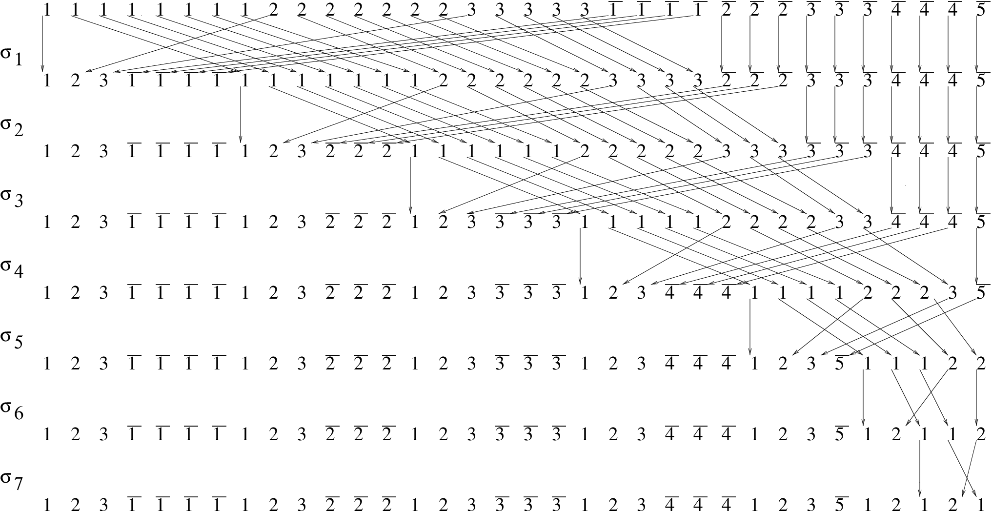
Now note that σT~−\sigma^{-}_{\widetilde{T}} maps the word wT~w_{\widetilde{T}} to the word wλ−w_{\lambda}^{-} by place permutation. We decompose σ−T~=σλ1⋯σ1\sigma^{-}_{\widetilde{T}}=\sigma_{\lambda_{1}}\cdots\sigma_{1}, so that ℓ⁡(σT~−)=ℓ⁡(σλ1)+⋯+ℓ⁡(σ1)\ell\left(\sigma^{-}_{\widetilde{T}}\right)=\ell\left(\sigma_{\lambda_{1}}\right)+\cdots+\ell\left(\sigma_{1}\right) as in the followings ways:

First we define a sequence T~0=T~,T~1,…,T~λ2−1,T~λ2=Sλ−\widetilde{T}_{0}=\widetilde{T},\widetilde{T}_{1},\ldots,\widetilde{T}_{\lambda_{2}-1},\widetilde{T}_{\lambda_{2}}=S_{\lambda}^{-} of standard tableux such that T~i\widetilde{T}_{i} is a standard tableau of shape λ\lambda whose entries increase by one down the first ii columns, and then other entries increase by one just like they are in the T~\widetilde{T} for the rest of columns, i.e. entries increase by one across rows for first mm rows then entries increase by on down the columns. Then we define σi:=σT~i−1T~i\sigma_{i}:=\sigma_{\widetilde{T}_{i-1}}^{\widetilde{T}_{i}}.

We give an example to explain our idea. If

λ=(λ1,λ2)=[Uncaptioned image]∈H⁡(3,5),\lambda=(\lambda^{1},\lambda^{2})=\rotatebox[origin]{270.0}{\rotatebox[origin]{90.0}{\scalebox{0.35}{\includegraphics[]{foo2.eps}}}}\in H(3,5),

then T~0=T~\widetilde{T}_{0}=\widetilde{T}, T~1\widetilde{T}_{1}, T~2\widetilde{T}_{2}, T~3\widetilde{T}_{3}, T~4\widetilde{T}_{4}, T~5\widetilde{T}_{5}, T~6\widetilde{T}_{6}, and T~7=Sλ−\widetilde{T}_{7}=S^{-}_{\lambda} are

T~0=[Uncaptioned image],\displaystyle\widetilde{T}_{0}=\rotatebox[origin]{270.0}{\rotatebox[origin]{90.0}{\scalebox{0.35}{\includegraphics[]{tildh38.eps}}}},\qquad T~1=[Uncaptioned image]\displaystyle\widetilde{T}_{1}=\rotatebox[origin]{270.0}{\rotatebox[origin]{90.0}{\scalebox{0.35}{\includegraphics[]{t1.eps}}}}
T~2=[Uncaptioned image],\displaystyle\widetilde{T}_{2}=\rotatebox[origin]{270.0}{\rotatebox[origin]{90.0}{\scalebox{0.35}{\includegraphics[]{t2.eps}}}}, T~3=[Uncaptioned image],\displaystyle\widetilde{T}_{3}=\rotatebox[origin]{270.0}{\rotatebox[origin]{90.0}{\scalebox{0.35}{\includegraphics[]{t3.eps}}}},
T~6=[Uncaptioned image],\displaystyle\widetilde{T}_{6}=\rotatebox[origin]{270.0}{\rotatebox[origin]{90.0}{\scalebox{0.35}{\includegraphics[]{t6.eps}}}}, T~7=[Uncaptioned image].\displaystyle\widetilde{T}_{7}=\rotatebox[origin]{270.0}{\rotatebox[origin]{90.0}{\scalebox{0.35}{\includegraphics[]{tminus.eps}}}}.

And our decomposition σ−T~=σ7⋯σ1\sigma^{-}_{\widetilde{T}}=\sigma_{7}\cdots\sigma_{1} is illustrated in Figure 1.

Refer to caption
Figure 1. σ−T~=σ7⋯σ1\sigma^{-}_{\widetilde{T}}=\sigma_{7}\cdots\sigma_{1}

Note the i¯\overline{i}’s entries of our wT~′w^{\prime}_{\widetilde{T}} and wλ−′w^{\prime}_{\lambda_{-}} are not nicely ordered as in Figur 1, but we don’t need to consider those orders.

Now we notice that the situation explained in (4.3) does not happen in decomposition σ−T~=σ7⋯σ1\sigma^{-}_{\widetilde{T}}=\sigma_{7}\cdots\sigma_{1}, because once an entry moves to the left, then it is fixed by the following series of transformations σl\sigma_{l} so that it goes straight down, and it does not produce any further crossings of edges. This is clear from Figure 1. Thus

ℓ(σλ2⋯σ1)=ℓ(σλ2)+⋯+ℓ(σ1),\ell(\sigma_{\lambda_{2}}\cdots\sigma_{1})=\ell(\sigma_{\lambda_{2}})+\cdots+\ell(\sigma_{1}),

and so,

h(σλ2⋯σ1)=h(σλ2)⋯h(σ1).h(\sigma_{\lambda_{2}}\cdots\sigma_{1})=h(\sigma_{\lambda_{2}})\cdots h(\sigma_{1}).

Next we decompose each σl\sigma_{l} into a product of transpositions. For example a decomposition for σ4\sigma_{4} in Figure 1 is explained in Figure 2.

Refer to caption

.

Figure 2. Decomposition of σ4\sigma_{4} into a product of transpositions

If each σl\sigma_{l} is expressed as a product τs1τs2⋯τsl\tau_{s_{1}}\tau_{s_{2}}\cdots\tau_{s_{l}} of transpositions as shown in Figure 2, then the expression is reduced for the same reason as decomposition in Figure 1 is reduced. So Hecke element h⁡(σl)h(\sigma_{l}) is also a product of hsh_{s}’s which correspond to the transpositions in the decomposition. Note also that we only exchange ii and i−1i-1 or ii and j¯\overline{j} during the process of applying the above place permutations.

Because Rˇ{\check{R}} maps tj⊗tit_{j}\otimes t_{i} to q​ti⊗tjqt_{i}\otimes t_{j} for i<ji<j and uj⊗tiu_{j}\otimes t_{i} to q​ti⊗ujqt_{i}\otimes u_{j}, we have

Rˇ−1:\displaystyle{\check{R}}^{-1}:\quad ti⊗tj\displaystyle t_{i}\otimes t_{j} ↦q−1​tj⊗ti,\displaystyle\mapsto q^{-1}t_{j}\otimes t_{i}, i<j\displaystyle\quad i<j ,
ti⊗uj\displaystyle t_{i}\otimes u_{j} ↦q−1​uj⊗ti,\displaystyle\mapsto q^{-1}u_{j}\otimes t_{i},\qquad for all i,ji,j .

Thus the actions of (hs)−1(h_{s})^{-1} coming from the decomposition of (h⁡(σ−T~))−1\left(h(\sigma^{\widetilde{T}}_{-})\right)^{-1} on the simple tensor wT~′w^{\prime}_{\widetilde{T}} are the same as the place permutations except for scalar multiples. Thus we have (h⁡(σ−T~))−1\left(h(\sigma^{\widetilde{T}}_{-})\right)^{-1} maps (5.11) to wλ−′w^{\prime}_{\lambda_{-}} except for a scalar multiple of a power of q−1q^{-1}. Hence (h⁡(σ−T~))−1​h​(σ+T~)​eλ+​wλ+\bigl(h(\sigma^{\widetilde{T}}_{-})\bigr)^{-1}h(\sigma^{\widetilde{T}}_{+})e^{+}_{\lambda}w_{\lambda}^{+} is a linear sum of

(5.13) 1⊗2⊗⋯⊗m⊗∗¯⊗⋯∗¯⏟(λ2)1⊗1⊗⋯⊗m⊗∗¯⊗⋯⊗∗¯⏟(λ2)2⊗⋯⊗1⊗⋯⊗λ2⊗1⊗⋯⊗1⏟λ1−λ2\begin{split}&1\otimes 2\otimes\cdots\otimes m\otimes{\underbrace{\overline{*}\otimes\cdots\overline{*}}_{(\lambda^{2})_{1}}}\otimes 1\otimes\cdots\otimes m\otimes{\underbrace{\overline{*}\otimes\cdots\otimes\overline{*}}_{(\lambda^{2})_{2}}}\\ &\quad\otimes\cdots\otimes 1\otimes\cdots\otimes\lambda_{2}\otimes\underbrace{1\otimes\cdots\otimes 1}_{\lambda_{1}-\lambda_{2}}\end{split}

Now we show that eλ−​wλ−′e^{-}_{\lambda}w^{\prime}_{\lambda_{-}} is killed by the action of ρ⊗k​(Ei)\rho^{\otimes k}\left(E_{i}\right) for i≤mi\leq m. The action of EiE_{i} on V⊗kV^{\otimes k} commute with the actions of the Hecke algebra, so that ρ⊗k​(Ei)​eλ−​wλ−′=eλ−​ρ⊗k​(Ei)​wλ−′\rho^{\otimes k}(E_{i})e_{\lambda}^{-}w^{\prime}_{\lambda_{-}}=e_{\lambda}^{-}\rho^{\otimes k}(E_{i})w^{\prime}_{\lambda_{-}}. Note ρ⊗k​(Ei)​wλ−′\rho^{\otimes k}(E_{i})w^{\prime}_{\lambda_{-}} is a linear sum of simple tensors θα\theta_{\alpha} such that each θα\theta_{\alpha} has a tensor factor where tit_{i} has been changed to ti−1t_{i-1} or u1u_{1} has been changed to tmt_{m}. If the first case happens, then there is a (j​j+1)∈C⁡(S−)(j\,j+1)\in C(S_{-}) such that hj​θα=q2​θαh_{j}\theta_{\alpha}=q^{2}\theta_{\alpha} (note Rˇ​(ti⊗ti)=q2​ti⊗ti{\check{R}}(t_{i}\otimes t_{i})=q^{2}t_{i}\otimes t_{i}). So

eλ−​θα=\displaystyle e^{-}_{\lambda}\theta_{\alpha}= q−2​eλ−​hj​θα\displaystyle q^{-2}e^{-}_{\lambda}h_{j}\theta_{\alpha}
=\displaystyle= q−2​(−1)​eλ−​θα.\displaystyle q^{-2}(-1)e^{-}_{\lambda}\theta_{\alpha}.

Hence we obtain eλ−​θα=0e^{-}_{\lambda}\theta_{\alpha}=0 as expected.

If the second case happens, then for some 1≤a,b≤k1\leq a,b\leq k, where a,ba,b are in the same column of S−S_{-}, the vectors in the aa’th and bb’th tensor slots are both tmt_{m}. Note the vectors between the aa’th and bb’th tensor slots are from {u1,…,un}\{u_{1},\ldots,u_{n}\}. Consider Hecke element haha+1⋯hb−2hb−1(hb−2)−1⋯(ha)−1∈ℋk(q2)h_{a}h_{a+1}\cdots h_{b-2}h_{b-1}(h_{b-2})^{-1}\cdots(h_{a})^{-1}\in{\mathcal{H}_{k}(q^{2})}. Without loss of generality we assume a=1a=1. Then

haha+1⋯\displaystyle h_{a}h_{a+1}\cdots hb−2hb−1(hb−2)−1⋯(ha)−1(tm⊗ui⊗⋯⊗uj⊗tm)\displaystyle h_{b-2}h_{b-1}(h_{b-2})^{-1}\cdots(h_{a})^{-1}(t_{m}\otimes u_{i}\otimes\cdots\otimes u_{j}\otimes t_{m})
=q−(b−a−2)haha+1⋯hb−2hb−1(ui⊗⋯⊗uj⊗tm⊗tm)\displaystyle=q^{-(b-a-2)}h_{a}h_{a+1}\cdots h_{b-2}h_{b-1}(u_{i}\otimes\cdots\otimes u_{j}\otimes t_{m}\otimes t_{m})
=q−(b−a−2)q2haha+1⋯hb−2(ui⊗⋯⊗uj⊗tm⊗tm)\displaystyle=q^{-(b-a-2)}q^{2}h_{a}h_{a+1}\cdots h_{b-2}(u_{i}\otimes\cdots\otimes u_{j}\otimes t_{m}\otimes t_{m})
=q−(b−a−2)q2q(b−a−2)(tm⊗ui⊗⋯⊗uj⊗tm)\displaystyle=q^{-(b-a-2)}q^{2}q^{(b-a-2)}(t_{m}\otimes u_{i}\otimes\cdots\otimes u_{j}\otimes t_{m})
=q2(tm⊗ui⊗⋯⊗uj⊗tm),\displaystyle=q^{2}(t_{m}\otimes u_{i}\otimes\cdots\otimes u_{j}\otimes t_{m}),

which explains that

haha+1⋯hb−2hb−1(hb−2)−1⋯(ha)−1θα=q2θα.h_{a}h_{a+1}\cdots h_{b-2}h_{b-1}(h_{b-2})^{-1}\cdots(h_{a})^{-1}\theta_{\alpha}=q^{2}\theta_{\alpha}.

Note eλ−​hj=−eλ−e^{-}_{\lambda}h_{j}=-e^{-}_{\lambda} and eλ−​(hj)−1=−eλ−e^{-}_{\lambda}(h_{j})^{-1}=-e^{-}_{\lambda} if sj∈C⁡(S−)s_{j}\in C(S_{-}), so that

eλ−​θα\displaystyle e^{-}_{\lambda}\theta_{\alpha} =q−2eλ−haha+1⋯hb−2hb−1(hb−2)−1⋯(ha)−1θα\displaystyle=q^{-2}e^{-}_{\lambda}h_{a}h_{a+1}\cdots h_{b-2}h_{b-1}(h_{b-2})^{-1}\cdots(h_{a})^{-1}\theta_{\alpha}
=−q−2​eλ−​θα.\displaystyle=-q^{-2}e^{-}_{\lambda}\theta_{\alpha}.

Therefore we have eλ−​θα=0e^{-}_{\lambda}\theta_{\alpha}=0 again this case. Hence Ei​i+1​eλ−​wλ′=0E_{i\,i+1}e_{\lambda}^{-}w^{\prime}_{\lambda}=0. And we have shown here ρ⊗k​(Ei)​v+=0\rho^{\otimes k}(E_{i})v_{+}=0 for 1≤i≤m1\leq i\leq m.

(ii) Second we consider the case m<i≤m+n−1m<i\leq m+n-1.

This case is somewhat easier than the other case. First note Ei,i+1​wλ+E_{i,i+1}w_{\lambda}^{+} is a linear sum of simple tensors θα\theta_{\alpha} such that one of ui+1u_{i+1} in tensor slots of wλ+w_{\lambda}^{+} is changed to uiu_{i}. Then for some (j​j+1)∈R⁡(S+)(j\,j+1)\in R(S_{+}), hj​θα=−θαh_{j}\theta_{\alpha}=-\theta_{\alpha} because Rˇ(ui⊗ui)=−ui⊗ui{\check{R}}(u_{i}\otimes u_{i})=-u_{i}\otimes u_{i}. Thus

eλ+​θα\displaystyle e^{+}_{\lambda}\theta_{\alpha} =−eλ+​hj​θα\displaystyle=-e^{+}_{\lambda}h_{j}\theta_{\alpha}
=−q2​eλ+​θα.\displaystyle=-q^{2}e^{+}_{\lambda}\theta_{\alpha}.

Thus we have eλ+​θα=0e^{+}_{\lambda}\theta_{\alpha}=0 and we have ρ⊗k​(Ei)​v+=0\rho^{\otimes k}(E_{i})v_{+}=0 for i≤mi\leq m as expected. ∎

Now from Proposition 2.18, Theorem 3.11, Corollary 3.12, the double centralizer theorem, and Theorem 5.5, we have

Theorem 5.14.

Let λ⊢k\lambda\vdash k be a partition in H⁡(m,n)H(m,n). Let TT be a standard tableau of shape λ\lambda. Then 𝔘q{\mathfrak{U}_{q}}-submodule yT​(q)​(V⊗k)y_{T}(q)(V^{\otimes k}) is isomorphic to the irreducible 𝔘q​(g​l​(m,n)){\mathfrak{U}_{q}(gl(m,n))}-module V⁡(λ)V(\lambda). Moreover as an ℋk​(q2)×𝔘q​(g​l​(m,n)){\mathcal{H}_{k}(q^{2})}\times{\mathfrak{U}_{q}(gl(m,n))} bimodule

V⊗k≃⨁λ⊢kλ∈H⁡(m,n)Hλ⊗V⁡(λ),V^{\otimes k}\simeq\bigoplus_{\begin{subarray}{c}\lambda\vdash k\\ \lambda\in H(m,n)\end{subarray}}H^{\lambda}\otimes V(\lambda),

where HλH^{\lambda} is the irreducible ℋk​(q2){\mathcal{H}_{k}(q^{2})}-module labeled by λ\lambda.

References

  • [1] G. Benkart, S. Kang, and M. Kashiwara. Crystal basis for the quantum superalgebra 𝒰q​(g​l​(m,n))\mathcal{U}_{q}(gl(m,n)). Journal of Amer. Math. Soc., 13:295–331, 2000.
  • [2] G. Benkart and C. Lee. Stability in modules for general linear Lie superalgebras. Nova Journal of Algebra and Geometry, 2(4):383–409, 1993.
  • [3] A. Berele and A. Regev. Hook Young diagrams with applications to combinatorics, and to representations of Lie superalgebras. Adv. in Math., 64:118–175, 1987.
  • [4] R. Floreanini, D. Leites, and L. Vinet. On the defining relations of quantum superalgebras. Lett. in Math. Physics, 23:127–131, 1991.
  • [5] F. Frobenius. Über die Charaktere der symmetricschen Gruppe. Preuss. Akad. Wiss. Sitz., pages 516–534, 1900. reprinted in Gesamelte Abhandlungen vol. 3, 148–166.
  • [6] A. Gyoja. A qq-analogue of Young symmetrizer. Osaka J. Math,, 23:841–852, 1986.
  • [7] M. Jimbo. A qq-analog of 𝒰⁡(g​l​(n+1))\mathcal{U}(gl(n+1)), Hecke algebra, and the Yang-Baxter equation. Lett. Math. Phys., 11:247–252, 1986.
  • [8] S.M. Khoroshkin and V.N. Tolstoy. Universal R{R}-matrix for quantized (super)algebras. Commun. Math. Phys., 141:599–617, 1991.
  • [9] R. Leduc and A. Ram. A Ribbon Hopf algebra approach to the irreducible representations of centralizer algebras:The Brauer Birman-Wenzl, and type A Iwahori-Hecke algebras. Adv. in Math., 125:1–94, 1997.
  • [10] G. Lusztig. On a theorem of Benson and Curtis. J. Algebra, 71:490–498, 1981.
  • [11] M. Scheunert. Serre-type relations for special linear Lie superalgebras. Lett. Math. Phys., 24:173–181, 1992.
  • [12] M. Scheunert. Presentation and qq deformation of Lie superalgebras. J. Math. Phys., 34:3780–3808, 1993.
  • [13] I. Schur. Über eine Klasse von Matrizen, die sich einer gegeben Matrix zuordenen lassen. PhD thesis, 1901. reprinted in Gesamelte Abhandlungen vol. 1, 1–70.
  • [14] I. Schur. Über die rationalen Darstellungen der allgemeinen linearen Gruppe. Preuss. Akad. Wiss. Sitz., pages 58–75, 1927. reprinted in Gesamelte Abhandlungen vol. 3, 68–85.
  • [15] A. Young. On Quantitative substitutional analysis i-ix, 1901–1952. reprinted in The Collected Papaers of Alfred Young 1873-1940, Mathematical Exposition No.21 U. of Toronto Press,(1977).