Morse theory on spaces of braids and Lagrangian dynamicsThanks: The first author was supported by NSF DMS-9971629 and NSF DMS-0134408. The second author was supported by an EPSRC Fellowship. The third author was supported by NWO Vidi-grant 639.032.202.
Abstract.
In the first half of the paper we construct a Morse-type theory on certain spaces of braid diagrams. We define a topological invariant of closed positive braids which is correlated with the existence of invariant sets of parabolic flows defined on discretized braid spaces. Parabolic flows, a type of one-dimensional lattice dynamics, evolve singular braid diagrams in such a way as to decrease their topological complexity; algebraic lengths decrease monotonically. This topological invariant is derived from a Morse-Conley homotopy index.
In the second half of the paper we apply this technology to second order Lagrangians via a discrete formulation of the variational problem. This culminates in a very general forcing theorem for the existence of infinitely many braid classes of closed orbits.
1. Prelude
It is well-known that under the evolution of any scalar uniformly parabolic equation of the form
| (1) |
the graphs of two solutions and evolve in such a way that the number of intersections of the graphs does not increase in time. This principle, known in various circles as “comparison principle” or “lap number” techniques, entwines the geometry of the graphs ( is a curvature term), the topology of the solutions (the intersection number is a local linking number), and the local dynamics of the PDE. This is a valuable approach for understanding local dynamics for a wide variety of flows exhibiting parabolic behavior with both classical [55] and contemporary [42, 6, 11, 20] implications.
This paper is an extension of this local technique to a global technique. One such well-established globalization appears in the work of Angenent on curve-shortening [5]: evolving closed curves on a surface by curve shortening isolates the classes of curves dynamically and implies a monotonicity with respect to number of self-intersections.
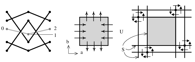
In contrast, one could consider the following topological globalization. Superimposing the graphs of a collection of functions gives something which resembles the projection of a topological braid onto the plane. Assume that the “height” of the strands above the page is given by the slope , or, equivalently, that all of the crossings in the projection are of the same sign (bottom-over-top): see Fig. 1[left]. Evolving these functions under a parabolic equation (with, say, boundary endpoints fixed) yields a flow on a certain space of braid diagrams which has a topological monotonicity: linking can be destroyed but not created. This establishes a partial ordering on the semigroup of positive braids which is respected by parabolic dynamics. The idea of topological braid classes with this partial ordering is a globalization of the lap number (which, in braid-theoretic terms becomes the length of the braid in the braid group under standard generators).
1.1. Parabolic flows on spaces of braid diagrams.
In this paper, we initiate the study of parabolic flows on spaces of braid diagrams. The particular braids in question will be (a) positive – all crossings are considered to be of the same sign; (b) closed11 1 The theory works equally well for braids with fixed endpoints. – the left and right sides are identified; and (c) discretized – or piecewise linear with fixed distance between “anchor points,” so as to avoid the analytic difficulties of working on infinite dimensional spaces of curves. See Fig. 1 for examples of braid diagrams.

The flows we consider evolve the anchor points of the braid diagram so that the braid class can change, but only so as to decrease complexity: local linking of strands may not increase with time. Due to the close similarity with parabolic partial differential equations such systems will be referred to as parabolic recurrence relations, and the induced flows as parabolic flows. These flows are given by
| (2) |
where the variables represent the vertical positions of the ordered anchor points of discrete braid diagrams. The only conditions imposed on the dynamics is the monotonicity condition that every be increasing functions of and .
While a discretization of a PDE of the form (1) with nearest-neighbor interaction yields a parabolic recurrence relation, the class of dynamics we consider is significantly larger in scope (see, e.g., [41]). Parabolic recurrence relations are a sub-class of monotone recurrence relations as studied in [4] and [27].
The evolution of braid diagrams yields a situation not unlike that considered by Vassiliev in knot theory [60]: in our scenario, the space of all braid diagrams is partitioned by the discriminant of singular diagrams into the braid classes. The parabolic flows we consider are transverse to these singular varieties (except for a set of “collapsed” braids) and are co-oriented in a direction along which the algebraic length of the braid decreases: this is an algebraic version of curve shortening.
To proceed, two types of noncompactness on spaces of braid diagrams must be repaired. Most severe is the problem of braid strands completely collapsing onto one another. To resolve this type of noncompactness, we assume that the dynamics fixes some collection of braid strands, a skeleton, and then work on spaces of braid pairs: one free, one fixed. The relative theory then leads to forcing results of the type “Given a stationary braid class, which other braids are forced as invariant sets of parabolic flows?” The second type of noncompactness in the dynamics occurs when the braid strands are free to evolve to arbitrarily large values. In the PDE setting, one requires knowledge of boundary conditions at infinity to prove theorems about the dynamics. In our braid-theoretic context, we convert boundary conditions to “artificial” braid strands augmented to the fixed skeleton.
Thus, working on spaces of braid pairs, the dynamics at the discriminant permits the construction of a Morse theory in the spirit of Conley to detect invariant sets of parabolic flows. Conley’s extension of the Morse index associates to any sufficiently isolated invariant set a space whose homotopy type measures not merely the dimension of the unstable manifold (the Morse index) but rather the coarse topological features of the unstable dynamics associated to this set. We obtain a well-defined Conley index for braid diagrams from the monotonicity properties of parabolic flows. To be more precise, relative braid classes (equivalence classes of isotopic braid diagrams fixing some skeleton) serve as candidates for isolating neighborhoods to which the Conley index can be assigned. This approach is reminiscent of the ideas of linking of periodic orbits used by Angenent [3, 5] and LeCalvez [37, 38].
Our finite-dimensional approximations to the (infinite-dimensional) space of smooth topological braids conceivably alter the Morse-theoretic properties of the discretized braid classes. One would like to know that so long as the discretization is not degenerately coarse, the homotopy index is independent of both the discretization and the specific parabolic flow employed. This is true. The principal topological result of this work is that the homotopy index is indeed an invariant of the topological (relative) braid class: see Theorems 19 and 20 for details. These theorems seem to evade a simple algebraic-topological proof. The proof we employ in §5 constructs the appropriate homotopy by recasting the problem into singular dynamics and applying techniques from singular perturbation theory.
We thus obtain a topological index which can, like the Morse index, force the existence of invariant sets. Specifically, a non-vanishing homotopy index for a relative braid class indicates that there is an invariant set in this braid class for any parabolic flow with the appropriate skeleton. This is the foundation for the applications to follow in the remainder of the paper.
The remainder of the paper explores applications of the machinery to a broad class of Lagrangian dynamics.
1.2. Second order Lagrangian dynamics.
Our principal application of the Morse theory on discretized braids is to the problem of finding periodic orbits of second order Lagrangian systems: that is, Lagrangians of the form where . An important motivation for studying such systems comes from the stationary Swift-Hohenberg model in physics, which is described by the fourth order equation
| (3) |
This equation is the Euler-Lagrange equation of the second order Lagrangian
| (4) |
We generalize to the broadest possible class of second order Lagrangians. One begins with the conventional convexity assumption, . The objective is to find bounded functions which are stationary for the action integral . Such functions are bounded solutions of the Euler-Lagrange equations
| (5) |
Due to the translation invariance , the solutions of (5) satisfy the energy constraint
| (6) |
where is the energy of a solution. To find bounded solutions for given values of , we employ the variational principle , which forces solutions of (5) to have energy . The Lagrangian problem can be reformulated as a two degree-of-freedom Hamiltonian system; in that context, bounded periodic solutions are closed characteristics of the (corresponding) energy manifold . Unlike the case of first-order Lagrangian systems, the energy hypersurface is not of contact type in general [7], and the recent stunning results in contact homology [17] are inapplicable.
The variational principle can be discretized for a certain considerable class of second order Lagrangians: those for which monotone laps between consecutive extrema are unique and continuous with respect to the endpoints. We give a precise definition in §8, denoting these as (second order Lagrangian) twist systems. Due to the energy identity (6) the extrema are restricted to the set , connected components of which are called interval components and denoted by . An energy level is called regular if for all satisfying . In order to deal with non-compact interval components certain asymptotic behavior has to be specified, for example that “infinity” is attracting. Such Lagrangians are called dissipative, and are most common in models coming from physics, like the Swift-Hohenberg Lagrangian. For a precise definition of dissipativity see §9. Other asymptotic behaviors may be considered as well, such as “infinity” is repelling, or more generally that infinity is isolating, implying that closed characteristics are a priori bounded in .
Closed characteristics are either simple or non-simple depending on whether , represented as a closed curve in the -plane, is a simple closed curve or not. This distinction is a sufficient language for the following general forcing theorem:
Theorem 1.
Any dissipative twist system possessing a non-simple closed characteristic at a regular energy value such that , must possess an infinite number of (non-isotopic) closed characteristics at the same energy level as .
This is the optimal type of forcing result: there are neither hidden assumptions about nondegeneracy of the orbits, nor restrictions to generic behavior. Sharpness comes from the fact that there exist systems with finitely many simple closed characteristics at each energy level.
The above result raises the following question: when does an energy manifold contain a non-simple closed characteristic? In general the existence of such characteristics depends on the geometry of the energy manifold. One geometric property that sparks the existence of non-simple closed characteristics is a singularity or near-singularity of the energy manifold. This, coupled with Theorem 1, triggers the existence of infinitely many closed characteristics. The results that can be proved in this context (dissipative twist systems) give a complete classification with respect to the existence of finitely many versus infinitely many closed characteristics on singular energy levels. The first result in this direction deals with singular energy values for which .
Theorem 2.
Suppose that a dissipative twist system has a singular energy level with , which contains two or more rest points. Then the system has infinitely many closed characteristics at energy level .22 2 From the proof of this theorem in §9 it follows that the statement remains true for energy values , with small.
Complementary to the above situation is the case when contains exactly one rest point. To have infinitely many closed characteristics, the nature of the rest point will come into play. If the rest point is a center (four imaginary eigenvalues), then the system has infinitely many closed characteristics at each energy level sufficiently close to , including . If the rest point is not a center, there need not exist infinitely many closed characteristics as results in [58] indicate.
Similar results can be proved for compact interval components (for which dissipativity is irrelevant) and semi-infinite interval components .
Theorem 3.
Suppose that a dissipative twist system has a singular energy level with an interval component , or , which contains at least one rest point of saddle-focus/center type. Then the system has infinitely many closed characteristics at energy level .
If an interval component contains no rest points, or only degenerate rest points (0 eigenvalues), then there need not exist infinitely many closed characteristics, completing our classification.
This classification immediately applies to the Swift-Hohenberg model (3), which is a twist system for all parameter values . We leave it to the reader to apply the above theorems to the different regimes of .
1.3. Additional applications
The framework of parabolic recurrence relations that we construct is robust enough to accommodate several other important classes of dynamics.
1.3.1. First-order nonautonomous Lagrangians
Finding periodic solutions of first-order Lagrangian systems of the form , with being 1-periodic in , can be rephrased in terms of parabolic recurrence relations of gradient type. The homotopy index can be used to find periodic solutions in this setting, even though a globally defined Poincaré map on need not exist.
1.3.2. Monotone twist maps
1.3.3. Uniformly parabolic PDE’s
1.3.4. Lattice dynamics
The form of a parabolic recurrence relation is precisely that arising from a set of coupled oscillators on a [periodic] one-dimensional lattice with nearest-neighbor attractive coupling. A similar setup arises in Aubry-LeDaeron-Mather theory of the Frenkel-Kontorova model [8]. In this setting, a nontrivial homotopy index yields existence of invariant states (or stationary, in the exact context) within a particular braid class. Related physical systems (e.g., charge density waves on a 1-d lattice [46]) are also often reducible to parabolic recurrence relations.
1.4. History and outline
The history of our approach is the convergence of ideas from knot theory, the dynamics of annulus twist maps, and curve shortening. We have already mentioned the similarities with Vassiliev’s topological approach to discriminants in the space of immersed knots. From the dynamical systems perspective, the study of parabolic flows and gradient flows in relation with embedding data and the Conley index can be found in work of Angenent [3, 4, 5] and Le Calvez [37, 38] on area preserving twist maps. More general studies of dynamical properties of parabolic-type flows appear in numerous works: we have been inspired by the work of Smillie [54], Mallet-Paret and Smith [40], Hirsch [27], and, most strongly, the work of Angenent on curve shortening [5]. Many of our applications to finding closed characteristics of second order Lagrangian systems share similar goals with the programme of Hofer and his collaborators (see, e.g., [17, 28, 29]), with the novelty that our energy surfaces are all non-compact and not necessarily of contact type [7].
Clearly there is a parallel between the homotopy index theory presented here and Boyland’s adaptation of Nielsen-Thurston theory for braid types of surface diffeomorphisms [10]. An important difference is that we require compactness only at the level of braid diagrams, which does not yield compactness on the level of the domains of the return maps [if these indeed exist]. Another important observation is that the recurrence relations are sometimes not defined on all of , which makes it very hard if not impossible to rephrase the problem of finding periodic solutions in terms of fixed points of 2-dimensional maps.
There are three components of this paper: (a) the precise definitions of the spaces involved and flows constructed, covered in §2-§3; (b) the establishment of existence, invariance, and properties of the index for braid diagrams in §4-§7; and (c) applications of the machinery to second order Lagrangian systems §8-§10. Finally, §11 contains open questions and remarks.
Acknowledgments. The authors would like express special gratitude to Sigurd Angenent and Konstantin Mischaikow for numerous enlightening discussions. Special thanks to Madjid Allili for his computational work in the earliest stages of this work. Finally, the hard work of the referee has improved the paper in several respects, especially in the definitions of equivalent relative braid classes.
2. Spaces of discretized braid diagrams
2.1. Definitions
Recall the definition of a braid (see [9, 26] for a comprehensive introduction). A braid on strands is a collection of embeddings with disjoint images such that (a) ; (b) for some permutation ; and (c) the image of each is transverse to all planes . We will “read” braids from left to right with respect to the -coordinate. Two such braids are said to be of the same topological braid class if they are homotopic in the space of braids: one can deform one braid to the other without any intersections among the strands. There is a natural group structure on the space of topological braids with strands, , given by concatenation. Using generators which interchange the and strands (with a positive crossing) yields the presentation for :
| (7) |
Braids find their greatest applications in knot theory via taking their closures. Algebraically, the closed braids on strands can be defined as the set of conjugacy classes33 3 Note that we fix the number of strands and do not allow the Markov move commonly used in knot theory. in . Geometrically, one quotients out the range of the braid embeddings via the equivalence relation and alters the restriction (a) and (b) of the position of the endpoints to be , as in Fig. 1[center]. Thus, a closed braid is a collection of disjoint embedded loops in which are everywhere transverse to the -planes.
The specification of a topological braid class (closed or otherwise) may be accomplished unambiguously by a labeled projection to the -plane: a braid diagram. Any braid may be perturbed slightly so that pairs of strand crossings in the projection are transversal: in this case, a marking of or serves to indicate whether the crossing is “bottom over top” or “top over bottom” respectively. Fig. 1[center] illustrates a topological braid with all crossings positive.
2.2. Discretized braids
In the sequel we will restrict to a class of closed braid diagrams which have two special properties: (a) they are positive — that is, all crossings are of type; and (b) they are discretized, or piecewise linear diagrams with constraints on the positions of anchor points. We parameterize such diagrams by the configuration space of anchor points.
Definition 4.
The space of discretized period braids on strands, denoted , is the space of all pairs where is a permutation on elements, and is an unordered collection of strands, , satisfying the following conditions:
- (a)
Each strand consists of anchor points: .
- (b)
For all , one has
- (c)
The following transversality condition is satisfied: for any pair of distinct strands and such that for some ,
(8)
The topology on is the standard topology of on the strands and the discrete topology with respect to the permutation , modulo permutations which change orderings of strands. Specifically, two discretized braids and are close iff for some permutation one has close to (as points in ) for all , with .
Remark 5.
In Equation (8), and indeed throughout the paper, all expressions involving coordinates are considered mod the permutation at ; thus, for every , we recursively define
| (9) |
As a point of notation, subscripts always refer to the spatial discretization and superscripts always denote strands. For simplicity, we will henceforth suppress the portion of a discretized braid .
One associates to each configuration the braid diagram , given as follows. For each strand , consider the piecewise-linear (PL) interpolation
| (10) |
for . The braid diagram is then defined to be the superimposed graphs of all the functions , as illustrated in Fig. 1[right] for a period six braid on four strands (crossings are shown merely for suggestive purposes).
This explains the transversality condition of Equation (8): a failure of this equation to hold implies that there is a PL-tangency in the associated braid diagram. Since all crossings in a discretized braid diagram are PL-transverse, the map sends to a topological closed braid diagram once a convention for crossings is chosen. Inspired by lifting smooth curves to a 1-jet extension, we label all crossings of as positive type. This can be thought of as using the slope of the PL-extension of as the “height” of the braid strand (though this analogy breaks down at the sharp corners). With this convention, then, the space embeds into the space of all closed positive braid diagrams on strands.
Definition 6.
Two discretized braids are of the same discretized braid class, denoted , if and only if they are in the same path-component of . The topological braid class, , denotes the path component of in the space of positive topological braid diagrams.
The proof of the following lemma is essentially obvious.
Lemma 7.
If in , then the induced positive braid diagrams and correspond to isotopic closed topological braid diagrams.
The converse to this Lemma is not true: two discretizations of a topological braid are not necessarily connected in .
Since one can write the generators of the braid group as elements of , it is clear that all positive topological braids are representable as discretized braids. Likewise, the relations for the groups of positive closed braids can be accomplished by moving within the space of discretized braids; hence, this setting suffices to capture all the relevant braid theory we will use.
2.3. Singular braids
The appropriate discriminant for completing the space consists of those “singular” braid diagrams admitting tangencies between strands.
Definition 8.
Denote by the -dimensional vector space44 4 Strictly speaking is not a vector space, but a union of vector spaces. Fixing appropriate permutations its components are vector spaces. Consider for instance which is a union of 3 copies of . of all discretized braid diagrams which satisfy properties (a) and (b) of Definition 4. Denote by the set of singular discretized braids.
We will often suppress the period and strand data and write for the space of singular discretized braids. It follows from Definition 4 and Equation (8) that the set is a semi-algebraic variety in . Specifically, for any singular braid there exists an integer and indices such that , and
| (11) |
where the subscript is always computed mod the permutation at . The number of such distinct occurrences is the codimension of the singular braid diagram . We decompose into the union of strata graded by , the codimension of the singularity.
Any closed braid (discretized or topological) is partitioned into components by the permutation . Geometrically, the components are precisely the connected components of the closed braid diagram. In our context, a component of a discretized braid can be specified as , since, by our indexing convention, “wraps around” to the other side of the braid when .
For singular braid diagrams of sufficiently high codimension, entire components of the braid diagram can coalesce. This can happen in essentially two ways: (1) a single component involving multiple strands can collapse into a braid with fewer numbers of strands, or (2) distinct components can coalesce into a single component. We define the collapsed singularities, , as follows:
Clearly the codimension of singularities in is at least . Since for braid diagrams in the number of strands reduces, the subspace may be decomposed into a union of the spaces for ; i.e., . If , then .
2.4. Relative braid classes
Evolving certain components of a braid diagram while fixing the remaining components motivates working with a class of “relative” braid diagrams.
Given and , the union is naturally defined as the unordered union of the strands. Given , define
fixing and imposing transversality. The path components of comprise the relative discrete braid classes, denoted . The braid will be called the skeleton henceforth. The set of singular braids are those braids such that The collapsed singular braids are denoted by . As before, the set is the closure of in , and is denoted . We denote by the topological relative braid class: the set of topological (positive, closed) braids such that is a topological (positive, closed) braid diagram.
Given two relative braid classes and in and respectively, to what extend are they the same? Consider the set
The natural projection from to has as its fiber the braid class . The path component of in will be denoted . This generates the equivalence relation for relative braid classes to be used in the remainder of this work: if and only if .
Likewise, define to be the set of equivalent topological relative braid classes. That is, if and only if there is a continuous family of topological (positive, closed) braid diagram pairs deforming to .
3. Parabolic recurrence relations
We consider the dynamics of vector fields given by recurrence relations on the spaces of discretized braid diagrams. These recurrence relations are nearest neighbor interactions — each anchor point on a braid strand influences anchor points to the immediate left and right on that strand — and resemble spatial discretizations of parabolic equations.
3.1. Axioms and exactness
Denote by the sequence space .
Definition 9.
A parabolic recurrence relation on is a sequence of real-valued functions satisfying
- (A1):
-
[monotonicity]55 5 Equivalently, one could impose and for all . and for all
- (A2):
-
[periodicity] For some , for all .
For applications to Lagrangian dynamics a variational structure is necessary. At the level of recurrence relations this implies that is a gradient:
Definition 10.
A parabolic recurrence relation on is called exact if
- (A3):
-
[exactness] There exists a sequence of generating functions, , satisfying
(12) for all .
In discretized Lagrangian problems the action functional naturally defines the generating functions . This agrees with the “formal” action in this case: . In this general setting, .
3.2. The induced flow
In order to define parabolic flows we regard as a vector field on : consider the differential equations
| (13) |
Equation (13) defines a (local) flow on under any periodic boundary conditions with period . To define flows on the finite dimensional spaces , one considers the same equations:
| (14) |
where the ends of the braid are identified as per Remark 5. Axiom (A2) guarantees that the flow is well-defined. Indeed, one may consider a cover of by taking the bi-infinite periodic extension of the braids: this yields a subspace of periodic sequences in invariant under the product flow of (13) thanks to Axiom (A2). Any flow generated by (14) for some parabolic recurrence relation is called a parabolic flow on discretized braids. In the case of relative classes a parabolic flow is the restriction of a parabolic flow on which fixes the anchor points of the skeleton . We abuse notation and indicate the invariance of the skeleton by . Indeed, for appropriate coverings of the skeletal strands it holds that .
3.3. Monotonicity and braid diagrams
The monotonicity Axiom (A1) in the previous subsection has a very clean interpretation in the space of braid diagrams. Recall from §2 that any discretized braid has an associated diagram which can be interpreted as a positive closed braid. Any such diagram in general position can be expressed in terms of the (positive) generators of the braid group . While this word is not necessarily unique, the length of the word is, as one can easily see from the presentation of and the definition of . The length of a closed braid in the generators is thus precisely the word metric from geometric group theory. The geometric interpretation of for a braid is clearly the number of pairwise strand crossings in the diagram .
The primary result of this section is that the word metric acts as a discrete Lyapunov function for any parabolic flow on . This is really the braid-theoretic version of the lap number arguments that have been used in several related settings [3, 5, 6, 20, 23, 40, 42, 54]. The result we prove below can be excavated from these cited works; however, we choose to give a brief self-contained proof for completeness.
Proposition 11.
Let be a parabolic flow on .
- (a)
For each point , the local orbit intersects uniquely at for all sufficiently small.
- (b)
For any such , the length of the braid diagram for in the word metric is strictly less than that of the diagram , .
Proof. Choose a point in representing a singular braid diagram. We induct on the codimension of the singularity. In the case where (i.e., ), there exists a unique and a unique pair of strands such that and
Note that the inequality is strict since . We deduce from (14) that
From Axiom (A2) one has that
Therefore, as , the two strands have two local crossings, and as , these two strands are locally unlinked (see Fig. 2): the length of the braid word in the word metric is thus decreased by two, and the flow is transverse to . This proves (a) and (b) on .

Assume inductively that (a) and (b) are true for every point in for . To prove (a) on , choose . There are exactly distinct pairs of anchor points of the braid which coalesce at the braid diagram . Since the vector field is defined by nearest neighbors, singularities which are not strandwise consecutive in the braid behave independently to first order under the parabolic flow. Thus, it suffices to assume that for some , , and one has and chains of consecutive anchor points for the braid diagram such that if and only if . (Recall that the addition is always done modulo the permutation at ). Then since
it follows that for all , the anchor points and are not separated to first order. At the left “end” of the singular braid, where ,
so that the vector field is tangent to at but is not tangent to : the flowline through decreases codimension immediately. By the induction hypothesis on (b), the flowline through cannot possess intersections with for which accumulate onto — the length of the braids are finite. Thus the flowline intersects locally at uniquely. This concludes the proof of (a).
It remains to show that the length of the braid word decreases strictly at in . By (a), the flow is nonsingular in a neighborhood of ; thus, by the Flowbox Theorem, there is a tubular neighborhood of local -flowlines about . The beginning and ending points of these local flowlines all represent nonsingular diagrams with the same word lengths as the beginning and endpoints of the path through , since the complement of is an open set. Since is a codimension- algebraic semi-variety in , it follows from transversality that most of the nearby orbits intersect , at which braid word length strictly decreases. This concludes the proof of (b).
To put this result in context with the literature, we note that the monotonicity in [23, 40] is one-sided: translated into our terminology, for all . One can adapt this proof to generalizations of parabolic recurrence relations appearing in the work of Le Calvez [37, 38]: namely, compositions of twist symplectomorphisms of the annulus reversing the twist-orientation.
As pointed out above a parabolic flow on is a special case of a parabolic flow on with a fixed skeleton , and therefor the analogue of the above proposition for relative classes thus follows as a special case.

Remark 12.
The information that we derive from relative braid diagrams is more than what one can obtain from lap numbers alone (cf. [37]). Fig. 3 gives examples of two closed discretized relative braids which have the same set of pairwise intersection numbers of strands (or lap numbers) but which force very different dynamical behaviors. The homotopy invariant we define in the next section distinguishes these braids. The index of the first picture can be computed to be trivial, and the index for the second picture is computed in §10 to be nontrivial.
4. The homotopy index for discretized braids
Technical lemmas concerning existence of certain types of parabolic flows are required for showing the existence and well-definedness of the Conley index on braid classes. We relegate these results to Appendix A.
4.1. Review of the Conley index
We include a brief primer of the relevant ideas from Conley’s index theory for flows. For a more comprehensive treatment, we refer the interested reader to [48].
In brief, the Conley index is an extension of the Morse index. Consider the case of a nondegenerate gradient flow: the Morse index of a fixed point is then the dimension of the unstable manifold to the fixed point. In contrast, the Conley index is the homotopy type of a certain pointed space (in this case, the sphere of dimension equal to the Morse index). The Conley index can be defined for sufficiently “isolated” invariant sets in any flow, not merely for fixed points of gradients.
Recall the notion of an isolating neighborhood as introduced by Conley [12]. Let be a locally compact metric space. A compact set is an isolating neighborhood for a flow on if the maximal invariant set is contained in the interior of . The invariant set is then called a compact isolated invariant set for . In [12] it is shown that every compact isolated invariant set admits a pair such that (following the definitions given in [48]) (i) with a neighborhood of ; (ii) is positively invariant in ; and (iii) is an exit set for : given and such that , then there exists a for which and . Such a pair is called an index pair for . The Conley index, , is then defined as the homotopy type of the pointed space , abbreviated . This homotopy class is independent of the defining index pair, making the Conley index well-defined.
A large body of results and applications of the Conley index theory exists. We recall following [48] two foundational results.
- (a)
Stability of isolating neighborhoods: Any isolating neighborhood for a flow is an isolating neighborhood for all flows sufficiently -close to .
- (b)
Continuation of the Conley index: Let , be a continuous family of flows with a family of isolating neighborhoods. Define the parameterized flow on , and . If is an isolating neighborhood for the parameterized flow then the index is invariant under .
Since the homotopy type of a space is notoriously difficult to compute, one often passes to homology or cohomology. One defines the Conley homology66 6 In [15] Čech cohomology is used. For our purposes ordinary singular (co)homology always suffices. of to be , where is singular homology. To the homological Conley index of an index pair one can also assign the characteristic polynomial , where is the free rank of . Note that, in analogy with Morse homology, if , then there exists a nontrivial invariant set within the interior of . For more detailed description see §7.
4.2. Proper and bounded braid classes
From Proposition 11, one readily sees that complements of yield isolating neighborhoods, except for the presence of the collapsed singular braids , which is an invariant set in . For the remainder of this paper we restrict our attention to those relative braid diagrams whose braid classes prohibit collapse.
Fix , and consider the relative braid classes (topological) and (discretized).
Definition 13.
A topological relative braid class is proper if it is impossible to find a continuous path of braid diagrams for such that , defines a braid for all , and is a diagram where an entire component of the closed braid has collapsed onto itself or onto another component of or . A discretized relative braid class is called proper if the associated topological braid class is proper, otherwise, it is improper: see Fig. 4.
Definition 14.
A topological relative braid class is called bounded if there exists a uniform bound on all representatives of the equivalence class, i.e. on the strands (in ). A discrete relative braid class is called bounded if the set is bounded.
Note that if a topological class is bounded then the discrete class is bounded as well for any period. The converse does not always hold. Bounded braid classes possess a compactness sufficient to implement the Conley index theory without further assumptions. It is not hard either to see or to prove that properness and boundedness are well-defined properties of equivalence classes of braids.
-0.25,-0.75)(10.25,6.75)
4.3. Existence and invariance of the Conley index for braids
Theorem 15.
Suppose is a bounded proper relative braid class and is a parabolic flow fixing . Then the following are true:
- (a)
is an isolating neighborhood for the flow , which thus yields a well-defined Conley index ;
- (b)
The index is independent of the choice of parabolic flow so long as ;
- (c)
The index is an invariant of .
Definition 16.
The homotopy index of a bounded proper discretized braid class in is defined to be , the Conley index of the braid class with respect to some (hence any) parabolic flow fixing any representative of the skeletal braid class .
Proof. Isolation is proved by examining on the boundary . By Definition 13 and 14 the set is compact, and . Choose a point on . Proposition 11 implies that the parabolic flow locally intersects at alone and that furthermore its length in the braid group strictly decreases. This implies that under , the point exits the set either in forwards or backwards time (if not both). Thus, and (a) is proved.
Denote by the index of . To demonstrate (b), consider two parabolic flows and that satisfy all our requirements, and consider the isolating neighborhood valid for both flows. Construct a homotopy , , by considering the parabolic recurrence functions , where and give rise to the flows and respectively. It follows immediately that , for all ; therefore is an isolating neighborhood for with . Define , , to be the maximal invariant set in with respect to the flow . The continuation property of the Conley index completes the proof of (b).
Assume that , so that there is a continuous path , for , of braid pairs within between the two. From the proof of Lemma 57 in Appendix A, there exists a continuous family of flows , such that , for all . Item (a) ensures that is an isolating neighborhood for all . The continuity of implies that the set is an isolating neighborhood for the parameterized flow on . Therefore via the continuation property of the Conley index, is independent of , which completes the proof of Item (c).
4.4. An intrinsic definition
For any bounded proper relative braid class we can define its index intrinsically, independent of any notions of parabolic flows. Denote as before by the set within . The singular braid diagrams partition into disjoint cells (the discretized relative braid classes), the closures of which contain portions of . For a bounded proper braid class, is compact, and avoids .
To define the exit set , consider any point on . There exists a small neighborhood of in for which the subset consists of a finite number of connected components . Assume that . We define to be the set of for which the word metric is locally maximal on , namely,
| (15) |
We deduce that is an index pair for any parabolic flow for which , and thus by the independence of , the homotopy type gives the Conley index. The index can be computed by choosing a representative and determining and . A rigorous computer assisted approach exists for computing the homological index using cube complexes and digital homology [24].
4.5. Three simple examples
It is not obvious what the homotopy index is measuring topologically. Since the space has one dimension per free anchor point, examples quickly become complex.
Example 1: Consider the proper period-2 braid illustrated in Fig. 5[left]. (Note that deleting any strand in the skeleton yields an improper braid.) There is exactly one free strand with two anchor points (recall that these are closed braids and the left and right sides are identified). The anchor point in the middle, , is free to move vertically between the fixed points on the skeleton. At the endpoints, one has a singular braid in which is on the exit set since a slight perturbation sends this singular braid to a different braid class with fewer crossings. The end anchor point, () can freely move vertically in between the two fixed points on the skeleton. The singular boundaries are in this case not on the exit set since pushing across the skeleton increases the number of crossings.
Since the points and can be moved independently, the configuration space in this case is the product of two compact intervals. The exit set consists of those points on for which is a boundary point. Thus, the homotopy index of this relative braid is .
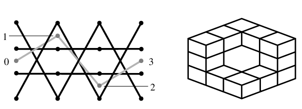
Example 2: Consider the proper relative braid presented in Fig. 6[left]. Since there is one free strand of period three, the configuration space is determined by the vector of positions of the anchor points. This example differs greatly from the previous example. For instance, the point (as represented in the figure) may pass through the nearest strand of the skeleton above and below without changing the braid class. The points and may not pass through any strands of the skeleton without changing the braid class unless has already passed through. In this case, either or (depending on whether the upper or lower strand is crossed) becomes free.
To simplify the analysis, consider as all of (allowing for the moment singular braids and other braid classes as well). The position of the skeleton induces a cubical partition of by planes, the equations being for the various strands of the skeleton . The braid class is thus some collection of cubes in . In Fig. 6[right], we illustrate this cube complex associated to , claiming that it is homeomorphic to . In this case, the exit set happens to be the entire boundary and the quotient space is homotopic to the wedge-sum .
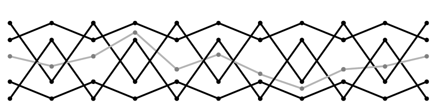
Example 3: To introduce the spirit behind the forcing theorems of the latter half of the paper, we reconsider the period two braid of Example 1. Take an -fold cover of the skeleton as illustrated in Fig. 7. By weaving a single free strand in and out of the strands as shown, it is possible to generate numerous examples with nontrivial index. A moment’s meditation suffices to show that the configuration space for this lifted braid is a product of intervals, the exit set being completely determined by the number of times the free strand is “threaded” through the inner loops of the skeletal braid as shown.
For an -fold cover with one free strand we can select a family of possible braid classes describes as follows: the even anchor points of the free strand are always in the middle, while for the odd anchor points there are three possible choices. Two of these braid classes are not proper. All of the remaining braid classes are bounded and have homotopy indices equal to a sphere for some . Several of these strands may be superimposed while maintaining a nontrivial homotopy index for the net braid: we leave it to the reader to consider this interesting situation.
Stronger results follow from projecting these covers back down to the period two setting of Example 1. If the free strand in the cover is chosen not to be isotopic to a periodic braid, then it can be shown via a simple argument that some projection of the free strand down to the period two case has nontrivial homotopy index. Thus, the simple period two skeleton of Example 1 is the seed for an infinite number of braid classes with nontrivial homotopy indices. Using the techniques of [33], one can use this fact to show that any parabolic recurrence relation () admitting this skeleton is forced to have positive topological entropy: cf. the related results from the Nielsen-Thurston theory of disc homeomorphisms [10].
5. Stabilization and invariance
5.1. Free braid classes and the extension operator
Via the results of the previous section, the homotopy index is an invariant of the discretized braid class: keeping the period fixed and moving within a connected component of the space of relative discretized braids leaves the index invariant. The topological braid class, as defined in §2, does not have an implicit notion of period. The effect of refining the discretization of a topological closed braid is not obvious: not only does the dimension of the index pair change, the homotopy types of the isolating neighborhood and the exit set may change as well upon changing the discretization. It is thus perhaps remarkable that any changes are correlated under the quotient operation: the homotopy index is an invariant of the topological closed braid class.
On the other hand, given a complicated braid, it is intuitively obvious that a certain number of discretization points are necessary to capture the topology correctly. If the period is too small may contain more than one path component with the same topological braid class:
Definition 17.
A relative braid class in is called free if
| (16) |
that is, if any other discretized braid in which has the same topological braid class as is in the same discretized braid class .
A braid class is free if the above definition is satisfied with . Not all discretized braid classes are free: see Fig. 8.

Define the extension map via concatenation with the trivial braid of period one (as in Fig. 9(a)):
| (17) |
The reader may note (with a little effort) that the non-equivalent braids of Fig. 8 become equivalent under the image of . There are exceptional cases in which is a singular braid when is not: see Fig. 9(b). If the intersections at are generic then is a nonsingular braid. One can always find such a representative in , again denoted by . Therefore the notation means that is chosen in with generic intersection at . The same holds for relative classes , i.e. choose such that all intersections of at are generic.

Note that under the action of boundedness of a braid class is not necessarily preserved, i.e. may be bounded, and unbounded. For this reason we will prove a stabilization result for topological bounded proper braid classes.
5.2. A topological invariant
Consider a period discretized relative braid pair which is not necessarily free. Collect all (a finite number) of the discretized braids such that the pairs are all topologically isotopic to but not pairwise discretely isotopic. For the case of a free braid class, .
Definition 18.
Given and as above, denote by the wedge of the homotopy indices of these representatives,
| (18) |
where is the topological wedge which, in this context, identifies all the constituent exit sets to a single point.
This wedge product is well-defined by Theorem 15 by considering the isolating neighborhood . In general a union of isolating neighborhoods is not necessarily an isolating neighborhood again. However, since the word metric strictly decreases at the invariant set decomposes into the union of invariant sets of the individual components of . Indeed, if an orbit intersects two components it must have passed through : contradiction.
The principal topological result of this paper is that H is an invariant of the topological bounded proper braid class .
Theorem 19.
Given and which are topologically isotopic as bounded proper braid pairs, then
| (19) |
The key ingredients in this proof are that (1) the homotopy index is invariant under (Theorem 19); and (2) discretized braids “converge” to topological braids under sufficiently many applications of (Proposition 27).
Theorem 20.
For any bounded proper discretized braid pair, the wedged homotopy index of Definition 18 is invariant under the extension operator:
| (20) |
Proof. By the invariance of the index with respect to the skeleton , we may assume that is chosen to have all intersections generic ( for all strands ). Thus, from the proof of Lemma 55 in Appendix A, we may fix a recurrence relation having as fixed point(s) for which .
For consider the one-parameter family of augmented recurrence functions77 7 Recall the indexing conventions: for a period braid, , and . on braids of period :
| (21) |
Because of our choice of as being independent of the first variable, is decoupled from the extension of the braid as wraps around to . By construction the above system satisfies Axioms (A1)-(A2) for all with, in particular, the strict monotonicity of (A1) holding only on one side. One therefore has a parabolic flow on for all . In the singular limit , this forces , and one obtains the flow .
Since the skeleton has only generic intersections, is a nonsingular braid. From Equation (21), all stationary solutions of are stationary solutions for , i.e., , for all . Notice that this is not true in general for non-constant solutions.
Denote by the subset of relative braids which are topologically isotopic to . Likewise, denote by the image under of the subset of braids in which are topologically isotopic to . In other words,
| (22) |
As per the paragraph preceding Definition 18, there are a finite number of connected components of each of these sets. Clearly, is a codimension- subset of . Since not all braids in have generic intersections, the set may tangentially intersect the boundary of . We will denote this set of -singular braids by : see Fig. 10.
By performing an appropriate change of coordinates (cf. [13]), we can recast the parabolic system as a singular perturbation problem. Let , with , and let , with . Upon rescaling time as , the vector field induced by our choice of is of the form
| (23) |
for some (unspecified) vector fields and with the functional dependence indicated. The product flow of this vector field (23) in the new coordinates is denoted by and is well-defined on . In the case , the set is a submanifold of fixed points containing for which the flow is transversally nondegenerate (since here ). By construction , as illustrated in Fig. 10 (in the simple case where all braid classes are free and is thus connected).

The remainder of the analysis is a technique in singular perturbation theory following [13]: one relates the -dynamics of Equation (23) to those of the -dynamics on , whose orbits are of the form , where satisfies the limiting equation . The Conley index theory is well-suited to this situation.
For any compact set and , let denote the “product” radius neighborhood in . Denote by the maximal value . Due to the specific form of (23), we obtain the following uniform squeezing lemma.
Lemma 21.
If is any invariant set of contained in some , then in fact . Moreover, for all points with and it holds that .
Proof. Let be an orbit in contained in some . Take the inner product of the -equation with :
Hence , and we conclude that if for some , then . Consequently grows unbounded for and therefore , a contradiction. Thus for all .
For points with and , the above inequality gives that .
By compactness of the proper braid class, it is clear that , and thus the maximal isolated invariant set of given by 88 8 Since is a proper braid class is contained in its interior., is strictly contained (and thus isolated) in for some compact and some sufficiently large. Fix as above. Lemma 21 now implies that as becomes small, is squeezed into — a small neighborhood of a compact subset of the critical manifold , as in Fig. 10.99 9 If one applies singular perturbation theory it is possible to construct an invariant manifold . The manifold lies strictly within and intersects at rest points of the .
This proximity of to allows one to compare the dynamics of the and flows. Let be an isolating neighborhood (isolating block with corners) for the maximal -dynamics invariant set within the braid class . Combining Lemma 21 above, Theorem 2.3C of [13], and the existence theorems for isolating blocks [61], one concludes that if is an index pair for the limiting equations then is an isolating block for for with sufficiently small. A suitable index pair for the flow of Equation (23) is thus given by
| (24) |
Clearly, then, the homotopy index of is equal to the homotopy index of for all sufficiently small. It remains to show that this captures the maximal invariant set .
Lemma 22.
For all sufficiently small , .
Proof. By the choice of it holds that . We start by proving that for sufficiently small. Assume by contradiction that for some sequence . Then, since is an isolating neighborhood for , there exist orbits in such that , for some . Define , and set . The sequence satisfies the equations
| (25) |
By assumption , and , for all and all . An Arzela-Ascoli argument then yields the existence of an orbit , with , satisfying the equation . By definition, , a contradiction, which proves that for sufficiently small.
The boundary of splits as , with
Since the compact set is contained in , the boundary component is contained in provided that is sufficiently small. If the set is non-empty then the boundary component never lies entirely in regardless of . As the set is contained is arbitrary small neighborhood of . Independent of the parabolic flow in question, and thus of , there exists a neighborhood of on which the co-orientation of the boundary is pointed inside the braid class . In other words for every parabolic system the points in enter under the flow, see Fig. 11.

By using coordinates and adapted to the singular strands, it it easily seen (Fig. 11) that the braids are simplified by moving into the set .
We now show that . If not, then there exist points for some sequence . Consider the -limit sets . Since , and since cannot enter in backward time due to the co-orientation of , it follows that is contained in .
By a similar Arzela-Ascoli argument as before, this yields a set which is invariant for the flow . However due to the form of the vector field the associated flow cannot contain an invariant set in , which proves that for sufficiently small.
Finally, knowing that , and that for sufficiently small it holds , it follows that , which proves the lemma.
Theorem 20 now follows. Since, by Theorem 15, the homotopy index is independent of the parabolic flow used to compute it, one may choose the parabolic flow for sufficiently small. The homotopy index of on the maximal invariant set yields the wedge of all the connected components: . We have computed that this index is equal to the index of on the original braid class: .
Remark 23.
The proof of Theorem 20 implies that any component of the period- braid class which does not intersect must necessarily have trivial index.
Remark 24.
The above procedure also yields a stabilization result for bounded proper classes which are not bounded as topological classes. In this case one simply augments the skeleton by two constant strands as follows. Define the augmented braid , where
| (26) |
Suppose is bounded for some period . It now holds that , and is a bounded class. It therefore follows from Theorem 19 that
| (27) |
where H can be evaluated via any discrete representative of of any admissible period.
5.3. Eventually free classes
At the end of this subsection, we complete the proof of Theorem 19. The preliminary step is to show that discretized braid classes are eventually free under .
Given a braid , consider the extension of period . Assume at first the simple case in which , so that is a period-2 braid. Draw the braid diagram as defined in §2 in the domain . Choose any 1-parameter family of curves such that and so that is transverse1010 10 At the anchor points, the transversality should be topological as opposed to smooth. to the braid diagram for all . Define the braid as follows:
| (28) |
The point is well-defined since is always transverse to the braid strands and intersects each strand but once.
Lemma 25.
For any such family of curves , .
Proof. It suffices to show that this path of braids does not intersect the singular braids . Since is assumed to be a nonsingular braid, every crossing of two strands in the braid diagram of is a transversal crossing between and . Thus, if for some , for distinct strands and , then
| (29) |
The braid has a crossing of the and strands at . Checking the transversality of this crossing yields
| (30) |
Thus the crossing is transverse and the braid is never singular.
Note that the proof of Lemma 25 does not require the braid to be a closed braid diagram since the isotopy fixes the endpoints: the proof is equally valid for any localized region of a braid in which one spatial segment has crossings and the next segment has flat strands.
Corollary 26.
The “shifted” extension operator which inserts a trivial period-1 braid at the discretization point in a braid has the same action on components of as does .

Proposition 27.
The period- discretized braid class is free when .
Proof. We must show that any braid which has the same topological type as is discretely isotopic to . Place both and in general position so as to record the sequences of crossings using the generators of the -strand positive braid semigroup, , as in §2. Recall the braid group has relations for and ; closure requires making conjugacy classes equivalent.
The conjugacy relation can be realized by a discrete isotopy as follows: since , must possess some discretization interval on which there are no crossings. Lemma 25 then implies that this interval without crossings commutes with all neighboring discretization intervals via discrete isotopies. Performing consecutive exchanges shifts the entire braid over by one discretization interval. This generates the conjugacy relation.
To realize the remaining braid relations in a discrete isotopy, assume first that and are of the form that there is at most one crossing per discretization interval. It is then easy to see from Fig. 12 that the braid relations can be executed via discrete isotopy.
In the case where (and/or ) exhibits multiple crossings on some discretization intervals, it must be the case that a corresponding number of other discretization intervals do not possess any crossings (since ). Again, by inductively utilizing Lemma 25, we may redistribute the intervals-without-crossing and “comb” out the multiple crossings via discrete isotopies so as to have at most one crossing per discretization interval.
Proof of Theorem 19: Assume that . This implies that there is a path of topological braid diagrams taking the pair to . This path may be chosen so as to follow a sequence of standard relations for closed braids. From the proof of Proposition 27, these relations may be performed by a discretized isotopy to connect the pair to for and sufficiently large, and of the right relative size to make the periods of both pairs equal. For this choice, then, , and their homotopy indices agree. An application of Theorem 20 completes the proof.
We suspect that all braids in the image of are free: a result which, if true, would simplify index computations yet further.
6. Duality
For purposes of computation of the index, we will often pass to the homological level. In this setting, there is a natural duality made possible by the fact that the index pair used to compute the index of a braid class can be chosen to be a manifold pair.
Definition 28.
The duality operator on discretized braids is the map given by
| (31) |
Clearly induces a map on relative braid diagrams by defining to be . The topological action of is to insert a half-twist at each spatial segment of the braid. This has the effect of linking unlinked strands, and, since is an involution, linked strands are unlinked by : see Fig. 13.

For the duality statements to follow, we assume that all braids considered have even periods and that all of the braid classes and their duals are proper, so that the homotopy index is well-defined.
Lemma 29.
The duality map respects braid classes: if then . Bounded braid classes are taken to bounded braid classes by .
Proof: It suffices to show that the map is a homeomorphism on the pair . This is true on since is a smooth involution (). If with and
| (32) |
then applying the operator yields points with each term in the above inequality multiplied by (if is even) or by (if is odd): in either case, the quantity is still non-negative and thus . Boundedness is clearly preserved.
Theorem 30.
- (a)
The effect of on the index pair is to reverse the direction of the parabolic flow.
- (b)
For of period with free strands,
(33) - (c)
For of period with free strands,
(34)
Proof: For (a), let denote an index pair associated to a proper relative braid class . Dualizing sends to a homeomorphic space . The following local argument shows that the exit set of the dual braid class is in fact the complement (in the boundary) of the exit set of the domain braid: specifically,
Let . At any singular anchor point of , i.e., where and the transversality condition is not satisfied, then it follows from Axiom (A2) that
| (35) |
(Depending on the form of (A2) employed, one might use on the right hand side without loss.) Since the subscripts on the left side have the opposite parity of the subscripts on the right side, taking the dual braid (which multiplies the anchor points by and respectively) alters the sign of the terms. Thus, the operator reverses the direction of the parabolic flow.
From this, we may compute the Conley index of the dual braid by reversing the time-orientation of the flow. Since one can choose the index pair used to compute the index to be an oriented manifold pair (specifically, an isolating block: see, e.g., [61]), one may then apply a Poincaré-Lefschetz duality argument as in [45] and use the fact that the dimension is to obtain the duality formula for homology. This yields (b).
The final claim (c) follows from (b) by showing that is bijective on topological braid classes within . Assume that and are distinct braid classes in of the same topological type. Since is a homeomorphism on , the dual classes and are distinct. Claim (c) follows upon showing that these duals are still topologically the same braid class.
Proposition 27 implies that for sufficiently large since . By Lemma 29,
which, by Lemma 7 means that these braids are topologically the same. The topological action of dualizing the -stabilizations of and is to add full twists. Since the full twist is in the center of the braid group (this element commutes with all other elements of the braid group [9]), one can factor the dual braids within the topological braid group and mod out by full twists, yielding that .
We use this homological duality to complete a crucial computation in the proof of the forcing theorems (e.g., Theorem 1) at the end of this paper. The following small corollary uses duality to give the first step towards answering the question of just what the homotopy index measures topologically about a braid class. Recall the definition of an augmented braid from Remark 24.
Corollary 31.
Consider the dual of any augmented proper relative braid. Adding a full twist to this dual braid shifts the homology of the index up by two dimensions.
Proof: Assume that is the dual of an augmented braid in period (the augmentation is required to keep the braid class bounded upon adding a full twist). The prior augmentation implies that the outer two strands of “maximally link” the remainder of the relative braid. The effect of adding a full twist to this braid can be realized by instead stabilizing twice and then dualizing. The homological duality implies that for each connected component of the topological class,
| (36) |
which gives the desired result for the index H via Theorem 30.
Remark 32.
Remark 33.
Given a braid class of odd period , the image under is not necessarily a discretized braid at all: without some symmetry condition, the braid will not “close up” at the ends. To circumvent this, define the dual of to be the braid — the dual of the period extension of . The analogue of Theorem 30 above is that
| (37) |
where sym denotes the subset of the braid class which consists of symmetric braids: for all .
7. Morse theory
It is clear that the Morse-theoretic content of the homotopy index on braids holds implications for the dynamics of parabolic flows and thus zeros of parabolic recurrence relations. With this in mind, we restrict ourselves to bounded proper braid classes.
Recall that the characteristic polynomial of an index pair is the polynomial
| (38) |
The Morse relations in the setting of the Conley index (see [15]) state that, if has a Morse decomposition into distinct isolating subsets , then
| (39) |
for some polynomial with nonnegative integer coefficients.
7.1. The exact, nondegenerate case
For parabolic recurrence relations which satisfy (A3) (gradient type) it holds that if , then has at least one fixed point in . Indeed, one has:
Lemma 34.
For an exact nondegenerate parabolic flow on a bounded proper relative braid class, the sum of the Betti numbers of , as defined in (38), is a lower bound on the number of fixed points of the flow on that braid class.
Proof: The details of this standard Morse theory argument are provided for the sake of completeness. Choose a nondegenerate gradient parabolic flow on (in particular, fixes for all time). Enumerate the [finite number of] fixed points of on this [bounded] braid class. By nondegeneracy, the fixed point set may be taken to be a Morse decomposition of . The characteristic polynomial of each fixed point is merely , where is the Morse co-index of . Substituting into Equation (39) yields the lower bound
| (40) |
On the level of the topological braid invariant H, one needs to sum over all the path components as follows. As in Theorem 19, choose period- representatives ( from 0 to ) for each path component of the topological class . If we consider fixed points in the union , we obtain the following Morse inequalities from (40) and Theorem 19:
| (41) |
where is the Betti number of . Thus, again, the sum of the Betti numbers is a lower bound, with the proviso that some components may not contain any critical points.
If the topological class is bounded the inequality (41) holds with the invariant .
7.2. The exact, degenerate case
Here a coarse lower bound still exists.
Lemma 35.
For an arbitrary exact parabolic flow on a bounded relative braid class, the number of fixed points is bounded below by the number of distinct nonzero monomials in the characteristic polynomial .
Proof: Assuming that is finite, all critical points are isolated and form a Morse decomposition of . The specific nature of parabolic recurrence relations reveals that the dimension of the null space of the linearized matrix at an isolated critical point is at most 2, see e.g. [57]. Using this fact Dancer proves [16], via the degenerate version of the Morse lemma due to Gromoll and Meyer, that for at most one index . Equation (39) implies that,
| (42) |
on the level of polynomials. As the result of Dancer implies that for each , , for some , it follows that the number of critical points needs to be at least the number of non-trivial monomials in .
As before, if we instead use the topological invariant H for we obtain that the number of monomials in is a lower bound for the total sum of fixed points over the topologically equivalent path-components.
More elaborate estimates in some cases can be obtained via the extension of the Conley index due to Floer [18].
7.3. The non-exact case
If we consider parabolic recurrence relations that are not necessarily exact, the homotopy index may still provide information about solutions of . This is more delicate because of the possibility of periodic solutions for the flow . For example, if , the index does not provide information about additional solutions for , as a simple counterexample shows. However, if then there exists at least one solution of with the specified relative braid class. Specifically,
Lemma 36.
An arbitrary parabolic flow on a bounded relative braid class is forced to have a fixed point if is nonzero. If the flow is nondegenerate, then the number of fixed points is bounded below by the quantity
| (43) |
Proof: Set . As the vector field has no zeros at , the Brouwer degree, , may be computed via a small perturbation and is given by1111 11 We choose to define the degree via in order to simplify the formulae.
For a generic perturbation the associated parabolic flow is a Morse-Smale flow [22]. The (finite) collection of rest points and periodic orbits of then yields a Morse decomposition of , and the Morse inequalities are
The indices of the fixed points are given by , where is the number of eigenvalues of with positive real part, and the indices of periodic orbits are given by . Upon substitution of we obtain
Thus, if the Euler characteristic of is non-trivial, then has at least one zero in .
In the generic case the Morse relations give even more information. One has , with , and . It then follows that , proving the stated lower bound.
The obvious extension of these results to the full index H is left to the reader.
8. Second order Lagrangian systems
In this final third of the paper, we apply the developed machinery to the problem of forcing closed characteristics in second order Lagrangian systems of twist type. The vast literature on fourth order differential equations coming from second order Lagrangians includes many physical models in nonlinear elasticity, nonlinear optics, physics of solids, Ginzburg-Landau equations, etc. (see §1). In this context we mention the work of [2, 39, 50, 51].
8.1. Twist systems
We recall from §1 that closed characteristics at an energy level are concatenations of monotone laps between minima and maxima , which are periodic sequences with even period . The extrema are restricted to the set , whose connected components are denoted by : interval components (see §1.2 for the precise definition). The problem of finding closed characteristics can, in most cases, be formulated as a finite dimensional variational problem on the extrema . The following twist hypothesis, introduced in [59], is key:
- (T):
has a minimizer for all , and and are -smooth functions of .
Here
Hypothesis (T) is a weaker version of the hypothesis that assumes that the monotone laps between extrema are unique (see, e.g., [35, 36, 59]). Hypothesis (T) is valid for large classes of Lagrangians . For example, if , the following two inequalities ensure the validity of (T):
- (a)
, and
- (b)
for all and .
Many physical models, such as the Swift-Hohenberg equation (3), meet these requirements, although these conditions are not always met. In those cases numerical calculations still predict the validity of (T), which leaves the impression that the results obtained for twist systems carry over to many more systems for which Hypothesis (T) is hard to check.1212 12 Another method to implement the ideas used in this paper is to set up a curve-shortening flow for second order Lagrangian systems in the plane. For these reasons twist systems play a important role in understanding second order Lagrangian systems. For a direct application of this see [32].
8.2. Discretization of the variational principle
We commence by repeating the underlying variational principle for obtaining closed characteristics as described in [59]. In the present context a broken geodesic is a -concatenation of monotone laps (alternating between increasing and decreasing laps) given by Hypothesis (T). A closed characteristic at energy level is a (-smooth) function , , which is stationary for the action with respect to variations , and , and as such is a ‘smooth broken geodesic’.
The following result, a translation of results implicit in [59], is the motivation and basis for the applications of the machinery in the first two-thirds of this paper.
Theorem 37.
Extremal points for bounded solutions of second order Lagrangian twist systems are solutions of an exact parabolic recurrence relation with the constraints that (i) ; and (ii) the recurrence relation blows up along any sequence satisfying .
Proof: For simplicity, we restrict to the case of a nonsingular energy level : for singular energy levels, a slightly more involved argument is required. Denote by the interior of , and by the diagonal. Then define the generating function
| (44) |
the action of the minimizing lap from to . That is a well-defined function is the content of Hypothesis (T). The action functional associated to for a period system is the function
Several properties of follow from [59]:
- (a)
[smoothness] .
- (b)
[monotonicity] for all .
- (c)
[diagonal singularity]
.
In general the function is strictly increasing in for all , and similarly is strictly increasing in . The function also has the additional property that .
Critical points of satisfy the exact recurrence relation
| (45) |
where is both well-defined and on the domains
by Property (a). The recurrence function is periodic with , as are the domains .1313 13 We could also work with sequences that satisfy . Property (b) implies that Axiom (A1) is satisfied. Indeed, , and .
Property (c) provides information about the behavior of at the diagonal boundaries of , namely,
| (46) |
The parabolic recurrence relations generated by second order Lagrangians are defined on the constrained polygonal domains .
Definition 38.
A parabolic recurrence relation is said to be of up-down type if (46) is satisfied.
8.3. Up-down restriction
The variational set-up for second order Lagrangians introduces a few complications into the scheme of parabolic recurrence relations as discussed in §2-§7. The problem of boundary conditions will be considered in the following section. Here, we retool the machinery to deal with the fact that maxima and minima are forced to alternate. Such braids we call up-down braids.1414 14 The more natural term alternating has an entirely different meaning in knot theory.
8.3.1. The space
Definition 39.
The spaces of general/nonsingular/singular up-down braid diagrams are defined respectively as:
Path components of comprise the up-down braid types , and path components in comprise the relative up-down braid types .
The set has a boundary in
| (47) |
Such braids, called horizontal singularities, are not included in the definition of since the recurrence relation (45) does not induce a well-defined flow on the boundary .
Lemma 40.
For any parabolic flow of up-down type on , the flow blows up in a neighborhood of in such a manner that the vector field points into . All of the conclusions of Theorem 15 hold upon considering the -closure of braid classes in , denoted
for all sufficiently small.
Proof: The proof that any parabolic flow of up-down type acts here so as to strictly decrease the word metric at singular braids is the same proof as used in Proposition 11. The only difficulty arises in what happens at the boundary of : we must show that respects the up-down restriction in forward time.
Define the function
Clearly, if , then . Let , and consider the evolution , . We compute as becomes small. Using (45) it follows that
These inequalities show that as soon as becomes too small. Due to the boundedness of and the infinite repulsion at , we can choose a uniform so that for , and thus is an isolating neighborhood for all .
8.3.2. Universality for up-down braids
We now show that the topological information contained in up-down braid classes can be continued to the canonical case described in §2. As always, we restrict attention to proper, bounded braid classes, proper being defined as in Definition 13, and bounded meaning that the set is bounded in . Note that an up-down braid class can sometimes be bounded while is not. To bounded proper up-down braids we assign a homotopy index. From Lemma 40 it follows that for sufficiently small the set is an isolating neighborhood in whose Conley index,
is well-defined with respect to any parabolic flow generated by a parabolic recurrence relation of up-down type, and is independent of . As before, non-triviality of implies existence of a non-trivial invariant set inside (see §8.3.3).
The obvious question is what relationship holds between the homotopy index and that of a braid class without the up-down restriction. To answer this, augment the skeleton as follows: define , where
The topological braid class is bounded and proper. Indeed, boundedness follows from adding the strands which bound , since . Properness is satisfied since is proper.
Theorem 41.
For any bounded proper up-down braid class in ,
Proof. From Lemma 55 in Appendix A we obtain a parabolic recurrence relation (not necessarily up-down type) for which is a solution. We denote the associated parabolic flow by . Define two functions and in , with , and for , , and for , , for some and to be specified later. Introduce a new recurrence function for odd, and for even. The associated parabolic flow will be denoted by , and by construction by choosing sufficiently small. Indeed, if we choose , the augmented skeleton is a fixed point for .
Since the braid class is bounded and proper, is an isolating neighborhood with invariant set Inv. If we choose large enough, and sufficiently small, then the invariant set Inv lies entirely in . Indeed, for large we have that for each , has a fixed sign on the complement of . Therefore, . Now restrict the flow to . We may now construct a homotopy between and , via (see Appendix A), where and the associated flow are defined by (45). The braid is stationary along the homotopy and therefore
which proves the theorem.
We point out that similar results can be proved for other domains with various boundary conditions. The key observation is that the up-down constraint is really just an addition to the braid skeleton.
8.3.3. Morse theory
For bounded proper up-down braid classes the Morse theory of §7 applies. Combining this with Lemma 40 and Theorem 41, the topological information is given by the invariant H of the topological braid type .
Corollary 42.
On bounded proper up-down braid classes, the total number of fixed points of an exact parabolic up-down recurrence relation is bounded below by the number of monomials in the critical polynomial of the homotopy index.
9. Multiplicity of closed characteristics
We now have assembled the tools necessary to prove Theorem 1, the general forcing theorem for closed characteristics in terms of braids, and Theorems 2 and 3, the application to singular and near-singular energy levels. Given one or more closed characteristics, we keep track of the braiding of the associated strands, including at will any period-two shifts. Fixing these strands as a skeleton, we add hypothetical free strands and compute the homotopy index. If nonzero, this index then forces the existence of the free strand as an existing solution, which, when added to the skeleton, allows one to iterate the argument with the goal of producing an infinite family of forced closed characteristics.
The following lemma (whose proof is straightforward and thus omitted) will be used repeatedly for proving existence of closed characteristics.
Lemma 43.
Assume that is a parabolic recurrence relation on with a solution. Then, for each integer , there exists a lifted parabolic recurrence relation on for which every lift of is a solution. Furthermore, any solution to the lifted dynamics on projects to some period- solution. 1515 15 This does not imply a -periodic solution, but merely a braid diagram of period .
The primary difficulties in the proof of the forcing theorems are (i) computing the index (we will use all features of the machinery developed thus far, including stabilization and duality); and (ii) asymptotics/boundary conditions related to the three types of closed interval components : a compact interval, the entire real line, and the semi-infinite ray.
All of the forcing theorems are couched in a little braid-theoretic language:
Definition 44.
The intersection number of two strands , of a braid is the number of crossings in the braid diagram, denoted
The trivial braid on strands is any braid (topological or discrete) whose braid diagram has no crossings whatsoever, i.e., , for all . The full-twist braid on strands, is the braid of connected components, each of which has exactly two crossings with every other strand, i.e., for all .
Among discrete braids of period two, the trivial braid and the full twist are duals in the sense of §6.
9.1. Compact interval components
Let be a regular energy level for which the set contains a compact interval component .
Theorem 45.
Suppose that a twist system with compact possesses one or more closed characteristics which, as a discrete braid diagram, form a nontrivial braid. Then there exists an infinity of non-simple, geometrically distinct closed characteristics in .
In preparation for the proof of Theorem 45 we state a technical lemma, whose [short] proof may be found in [59].
Lemma 46.
Let , then there exists a such that
- (1)
, , and
- (2)
, ,
for any .
Proof of Theorem 45. Via Theorem 37, finding closed characteristics is equivalent to solving the recurrence relation given by (45). Define the domains
For any integer denote by the set of -periodic sequences for which . By Lemma 46, choosing small enough forces the vector field to be everywhere transverse to , making positively invariant for the induced parabolic flow .
By Lemma 43, one can lift the assumed solution(s) to a pair of period single-stranded solutions to (45), and , satisfying , for some . Define the cones
The combination of the facts , Axiom (A1), and the behavior of on implies that on the boundaries of the cones and the vector field is everywhere transverse and pointing inward. Therefore, and are also positively invariant with respect to the parabolic flow . Consequently, has global maxima and on and respectively. The maxima and have the property that , . As a braid diagram, is a stationary skeleton for the induced parabolic flow .
Having found the solutions and we now choose a compact interval , such that the skeletal strands are all contained in . In this way we obtain a proper parabolic flow (circumventing boundary singularities) which can be extended to a parabolic flow on . Let be the relative braid class with a period free strand which links the strands and with intersection number while satisfying : see Fig. 14 below.

As an up-down braid class, is a bounded proper braid class provided , and the Morse theory discussed in §7 and §8.3.3 then requires the evaluation of the invariant H of the topological class . In this case, since , augmentation is not needed, and . The nontriviality of the homotopy index H is given by the following lemma, whose proof we delay until §10.
Lemma 47.
The Conley homology of is given by:
| (48) |
In particular .
From the Morse theory of Corollary 42 we derive that for each satisfying there exist at least two distinct period- solutions of (45), which generically are of index and . In this manner, the number of solutions depends on and . To construct infinitely many, we consider -fold coverings of the skeleton , i.e., one periodically extends to a skeleton contained in , . Now must satisfy . By choosing triples such that are relative prime, we obtain the same Conley homology as above, and therefore an infinity of pairs of geometrically distinct solutions of (45), which, via Lemma 43 and Theorem 37 yield an infinity of closed characteristics.
Note that if we set and , then the admissible ratios for finding closed characteristics are determined by the relation
| (49) |
Thus if and are maximally linked, i.e. , then closed characteristics exist for all ratios in .
9.2. Non-compact interval components:
On non-compact interval components, closed characteristics need not exist. An easy example of such a system is given by the quadratic Lagrangian , with . Clearly for all , and the Lagrangian system has no closed characteristics for those energy levels. For the existence of closed characteristics strongly depends on the eigenvalues of the linearization around . To treat non-compact interval components, some prior knowledge about asymptotic behavior of the system is needed. We adopt an asymptotic condition shared by most physical Lagrangians: dissipativity.
Definition 48.
A second order Lagrangian system is dissipative on an interval component if there exist pairs , with and arbitrarily large, such that
Dissipative Lagrangians admit a strong forcing theorem:
Theorem 49.
Suppose that a dissipative twist system with possesses one or more closed characteristic(s) which, as discrete braid diagram in the period-two projection, forms a link which is not a full-twist (Definition 44). Then there exists an infinity of non-simple, geometrically distinct closed characteristics in .
Proof. After taking the -fold covering of the period-two projection for some , the hypotheses imply the existence two sequences and that form a braid diagram in whose intersection number is not maximal, i.e. . Following Definition 48, choose , with such that for all , and let and be as in the proof of Theorem 45, with and playing the role of and respectively for some small. Furthermore define the set
Since , the vector field given by (45) is transverse to . Moreover, the set is contractible, compact, and is pointing outward at the boundary . The set is therefore negatively invariant for the induced parabolic flow . Consequently, there exists a global minimum in the interior of . Define the skeleton to be .
Consider the up-down relative braid class described as follows: choose to be a -periodic strand with , such that has intersection number with each of the strands , , as in Fig. 15. For , is a bounded proper up-down braid class. As before, in order to apply the Morse theory of Corollary 42, it suffices to compute the homology index of the topological braid class :
Lemma 50.
The Conley homology of is given by:
| (50) |
In particular .
By the same covering/projection argument as in the proof of Theorem 45, infinitely many solutions are constructed within the admissible ratios
| (51) |
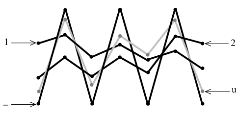
Theorem 49 also implies that the existence of a single non-simple closed characteristic yields infinitely many other closed characteristics. In the case of two unlinked closed characteristics all possible ratios in can be realized.
9.3. Half spaces
The case (or ) shares much with both the compact case and the the case . Since these are non-compact we again impose a dissipativity condition.
Definition 51.
A second order Lagrangian system is dissipative on an interval component if there exist arbitrarily large points such that
For dissipative Lagrangians we obtain the same general result as Theorem 45.
Theorem 52.
Suppose that a dissipative twist system with possesses one or more closed characteristics which, as a discrete braid diagram, form a nontrivial braid. Then there exists an infinity of non-simple, geometrically distinct closed characteristics in .
Proof. We will give an outline of the proof since the arguments are more-or-less the same as in the proofs of Theorems 45 and 49. Assume without loss of generality that . By assumption there exist two sequences and which form a nontrivial braid in , and thus . Defining the cone as in the proof of Theorem 45 yields a global maximum which contributes to the skeleton . Consider the braid class defined by adding the strand such that and links with the strands and with intersection number , .
Notice, in contrast to our previous examples, that is not bounded. In order to incorporate the dissipative boundary condition that is attracting, we add one additional strand . Set for even, and , for odd. As in the proof of Theorem 49 choose large enough such that . Let be a parabolic recurrence relation such that . Using one can construct yet another recurrence relation which coincides with on and which has as a fixed point (use cut-off functions). By definition the skeleton is stationary with respect to the recurrence relation .
Now let be as before, with the additional requirement that . This defines a bounded proper up-down braid class. The homology index of the topological class is given by the following lemma (see §10).
Lemma 53.
The Conley homology of is given by
| (52) |
In particular .
For the remainder of the proof we refer to that of Theorem 45.

9.4. A general multiplicity result and singular energy levels
9.4.1. Proof of Theorem 1
Lagrangians for which the above mentioned dissipativity conditions are satisfied for all (non-compact) interval components at energy , are called dissipative at .1616 16 One class of Lagrangians that is dissipative on all its regular energy levels is described by pointwise in . For such Lagrangians the results for the three different types of interval components are summarized in Theorem 1 in §1. The fact that the presence of a non-simple closed characteristic, when represented as a braid, yields a non-trivial, non-maximally linked braid diagram, allows us to apply all three Theorems 45, 49, and 52, proving Theorem 1.
9.4.2. Singular energy levels
The forcing theorems in §9.1 - §9.3 are applicable for all regular energy levels provided the correct configuration of closed characteristics can be found a priori. In this section we will discuss the role of singular energy levels; they may create configurations which force the existence of (infinitely) many periodic orbits. The equilibrium points in these singular energy levels act as seeds for the infinite family of closed characteristics.
For singular energy levels the set is the union of several interval components, for which at least one interval component contains an equilibrium point. If at an equilibrium point , then such a point is called non-degenerate and is contained in the interior of an interval component. For applying our results of the previous section the nature of the equilibrium points may play a role.
9.4.3. Case I:
We examine the case of a singular energy level such that and contains at least two equilibrium points. One observes that if the equilibria can be regarded as periodic orbits then Theorem 49 would apply: a regularization argument makes this rigorous. Let be the energy level in which is the concatenation of three interval components , i.e., the equilibria are and . We remark that the nature of the equilibrium points is irrelevant; there is a global reason for the existence of two unlinked periodic orbit in the energy levels for some small , see [59]. In these regular energy levels we can apply Theorem 49, and a limit procedure ensures that the periodic solutions persist to the degenerate energy level , proving Theorem 2.
Recall from [59] that two equilibrium points imply the existence of maximum and minimum , both simple closed characteristics, see Fig. 17. Define the regions , and , where is the point where the dissipativity condition of Definition 48 is satisfied. Then and .
-3.1,-3)(3,3.1) -3.1,-3)(3,3.1)
Since is a -function on it follows from Sard’s theorem that there exists a regular value such that . Consider the connected component of the super-level set which contains . The outer boundary of this component is a smooth circle and points inwards on this boundary circle. Let be the interior of the outer boundary circle in question. By continuity it follows that there exists a positive constant such that remains an isolating neighborhood for . In the following let be arbitrary.
Define . It follows from the properties of (see §8) that is again an isolating neighborhood, see Fig. 17. It holds that , and forms a Morse decomposition. The Morse relations (39) yield
where is a nonnegative polynomial. This implies that contains an index 1 solution . We can now define . In exactly the same way we find an index 1 solution . Notice, that by construction . Theorem 49 now yields an infinity of closed characteristics for all . As described in §9.2 these periodic solutions can be characterized by and , where is any pair of integers such that and and are relative prime (or ). Here is the period of the solution and .
In the limit the solutions and may collapse onto the two equilibrium points (if they are centers). Nevertheless, the infinite family of solutions still exists in the limit , because the extrema of the associated closed characteristics may only coalesce in pairs at the equilibrium points. This follows from the uniqueness of the initial value problem of the Hamiltonian system. Hence in the limit the type of the periodic solution is conserved when we count extrema with multiplicity and intersections without multiplicity.
Note that when the equilibria are saddle-foci then and stay away from in the limit . Extrema may still coalesce at the equilibrium points as , but intersections are counted with respect to and . Finally, in the regular energy levels , Theorem 49 provides at least two solutions of each type (except ); in the limit one cannot exclude the possibility that two solutions of the same type coincide.
Remark 54.
Theorem 2, proved in this subsection, is immediately applicable to the Swift-Hohenberg model (3) as described in §1. Notice that if the parameter satisifies , then Theorem 2 yields the existence of infinitely many closed chararacteristics at energy , and nearby levels. However from the physical point of view it is also of interest to consider the case . In that case there exists only one singular energy level and one equilibrium point. This case can be treated with our theory, but the nature of the equilibrium point comes into play. If an equilibrium point is a saddle or saddle-focus, it is possible that no additional periodic orbits exist (see [58]). However, if the equilibrium point is a center an initial non-simple closed characteristic can be found by analyzing an improper braid class, which by, Theorem 1, then yields infinitely many closed characteristics. The techniques involved are very similar to those used in the present and subsequent sections. We do not present the details here as this falls outside of the scope of this paper.
9.4.4. Cases II and III: or
The remaining cases are dealt with in Theorem 3. We will restrict the proof here to the case that contains an equilibrium point that is a saddle-focus — the center case can be treated as in [3].1717 17 Indeed, for energy levels , sufficiently small, a small simple closed charecteristic exists due to the center nature of the equilibrium point at ; spectrum , . This small simple closed characteristic will have a non-trivial rotation number close to . The fact that the rotation number is non-zero allows one to use the arguments in [3] to construct a non-simple closed characteristic. As a matter of fact a linked braid diagram is created this way. It also follows for the previous that there is no real difference between being compact or a half-line. For simplicity we consider the case that is compact.
-1.6,-1.5)(6.1,1.35)
Let us first make some preliminary observations. When is a saddle-focus, then in there exists a solution such that . This follows from the fact that there is a point , , close to at which the vector points to the north-west (see Fig. 18 and [59]). This solution is a saddle point, its rotation number being unknown. The impression is that is a minimum (with ), and if were a periodic solution, then one would have a linked pair and to which one could apply Theorem 45. Since is a saddle-focus it does not perturb to a periodic solution for . Hence we need to use a different regularization which conveys the information that acts as a minimum. The form of the perturbation that we have in mind is depicted in Fig. 18, where we have drawn the “potential” .
This idea can be formalized as follows. Choose a function such that , for , strictly decreases on and for . Add a perturbation
to the Lagrangian, i.e. , where . The new Euler-Lagrange equation near becomes
where all partial derivatives of are evaluated at , and where is the vector in phase space. Hence for all small there are now two additional equilibria near , denoted by and . Since , the difference between and is . To level this difference we add another small perturbation to of the form , i.e. , where is chosen so that (of course and shift slightly), and . Using the same analysis as before we conclude that a neighborhood of in the energy level looks just like Fig. 17. In we find a minimum. Choose an regular energy level slightly larger than (with , such that the minimum in persists. Taking this minimum and the original — which persists since we have only used small perturbations, preserving (see Fig. 18) as an isolating neighborhood — we apply Theorem 45.
Finally, we take the limit . The solutions now converge to solutions of the original equation in the degenerate energy level. It follows that in the energy level a solution of type exists, where the number of extrema has to be counted with multiplicity since extrema can coalesce in pairs at .
10. Computation of the homotopy index
Theorems 45, 49, and 52 hang on the homology computations of the homotopy invariant for certain canonical braid classes (Lemmas 47, 50, and 53). Our strategy (as in, e.g., [3]) is to choose a sufficiently simple system (an integrable Hamiltonian system) which exhibits the braids in question and to compute the homotopy index via knowing the structure of an unstable manifold. By the topological invariance of the homotopy index, any computable case suffices to give the index for any period .
Consider the first-order Lagrangian system given by the Lagrangian , where we choose to be an even four-well potential, with , and . The Lagrangian system defines an integrable Hamiltonian system on , with phase portrait given in Fig. 19.

Linearization about bounded solutions of the above Lagrangian system yields the quadratic form
which is strictly positive for all . For such choices of the time-1 map defined via the induced Hamiltonian flow , i.e., , is an area preserving monotone twist map. The generating function of the twist map is given by the minimization problem
where .1818 18 The strict positivity of the quadratic form via the choice of yields a smooth family of hyperbolic minimizers. The function is a smooth function on , with . The recurrence function satisfies Axioms (A1)-(A3), and thus defines an exact (autonomous) parabolic recurrence relation on . We choose the potential such that the bounded solutions within the heteroclinic loop between and have the property that the period is an increasing function of the amplitude , and , as .
This single integrable system is enough to compute the homotopy index of the three families of braid classes in Lemmas 47, 50, and 53 in §9.
We begin by identifying the following periodic solutions. Set , , and , . Let be a solution of with (minimum), , and , . For arbitrary this implies that
where we choose so that . For set and define , with , and , with , . Clearly, , for all .
Next choose , a solution of with (minimum), which oscillates around both equilibria and , and in between the equilibria and , and , . As before
Let and choose such that
Set , , and , with , . For the solutions and have exactly intersections. Therefore, if we choose sufficiently small, i.e. is large, then it also holds that .
Finally we choose the unique periodic solution , with , (minimum), and , . Let , and choose , and consequently the amplitude , so that
The solution is part of a hyperbolic circle of solutions , . Define , with , where . As before, since the intersection number of and is equal to , it holds that , for sufficiently small. Moreover, . From this point on is fixed. We now consider three different skeleta .
I: . The relative braid class is defined as follows: , and links with the strands and with intersection number , . The topological class is precisely that of Lemma 47 [Fig. 14] and as such is bounded and proper.
II: . The relative braid class is defined as follows: , links with the strands and with intersection number , , and links with with intersection number . The topological class is precisely that of Lemma 53 [Fig. 16] and as such is bounded and proper.
III: . The relative braid class is defined as follows: , links with the strands and with intersection number , and links with and with intersection number . The topological class is not bounded [Fig. 20[right]]. The augmentation of this braid class is bounded.
Cases I and II: Since the topological classes are bounded and proper, the invariant H is independent of period of the chosen representative, and can be easily computed from the integrable model. The closure of the collection of topologically equivalent braid classes is an isolating neighborhood for the parabolic flow induced by the recurrence relation (defined via ). The invariant set is given by the normally hyperbolic circle . For this reason the index H can be computed via the connected component that contains the critical circle; we denote this neighborhood by . The Conley index of can be determined via computing , the unstable manifold associated to this circle. This computation is precisely that appearing in the calculations of [3, pp. 372]: is orientable and of dimension , and thus
| (53) |
The Conley homology is given by for , and elsewhere. This completes the proofs of the Lemmas 47 and 53.
Case III: It holds that
The discrete class for period is bounded, but for periods this is not the case. However, by augmenting the braid, we obtain from (27) that
where . Since the topological class is bounded and proper, we may use the previous calculations to conclude that

Our motivation for this computation is to complete the proof of Lemma 50. Let denote the period braid class described by Fig. 15, with intersection numbers denoted by and , and let denote a type-III braid of period . Then, it is straightforward to see (as illustrated in Fig. 20) that, for and ,
| (54) |
Lemma 50 gives the index for the augmented class , which is bounded and proper as a topological class. The above considerations allow us to compute the homology of via Theorem 30:
| (55) |
The intersection numbers and are exactly those of Lemma 50, completing the proof.
11. Postlude
11.1. Extensions and questions: dynamics
There are several ways in which the basic machinery introduced in this paper can be generalized to other dynamical systems.
1. Scalar uniformly parabolic PDEs. Theorem 19 suggests strongly that the homotopy index for discretized braids extends to and agrees with an analogous index for parabolic dynamics on spaces of smooth curves via uniformly parabolic PDE’s. This is true [24].
2. Periodicity in the range. Although we consider the anchor points to be in , one may just as well constrain the anchor points to lie in and work in the universal cover. Such additional structure is used in the theory of annulus twist maps [3, 8, 37, 38, 43]. All of our results immediately carry over to this setting. We note that compact-type boundary conditions necessarily follow.
3. Aperiodic dynamics. One can also extend the theory to include braid diagrams with “infinite length” strands. To be more precise, consider braid diagrams on the infinite 1-d lattice, and omit the spatial periodicity. In this context several compactness issue come into play. To name a few: (a) the parabolic flows generated by aperiodic recurrence relations no longer live on a finite dimensional space but on the infinite dimensional space . See [3] for a case similar to this; (b) a priori, the Conley index should be replaced with an infinite dimensional analogue such as that developed by Rybakowski [53]. However, if one considers braid diagrams with finite word metric, the stabilization theory of §5 allows one to define the necessary invariants via the finite dimensional theory in this paper. This is not unlike the procedure one can follow in the treatment of parabolic PDE’s [24].
4. Fixed boundary conditions. Our decision to use closed braid diagrams is motivated by applications in Lagrangian systems; however, one can also fix the end points of the braid diagrams. In this setting one can define a braid invariant in the same spirit as is done for closed braids. The proof of stabilization is not sensitive to the type of boundary conditions used. Such an extension of the theory to include fixed endpoints is useful in applications to parabolic PDE’s [24].
5. Traveling waves and period orbits. The stationary solutions we find in this paper are but the beginnings of a dynamical skeleton for the systems considered. The next logical step would be to classify connecting orbits between stationary solutions: several authors (e.g., [41]) have considered these problems analytically in the context of traveling wave phenomena in monotone lattice dynamics. There is a precedent of using Conley indices to prove existence theorems for connecting orbits (e.g., [48]): we anticipate that such applications are possible in our setting. One could as well allow the skeletal strands to be part of a periodic motion (in the case of non-exact recurrence relations). In this setting one could look for both fixed points and periodic solutions of a given braid class.
6. Long-range coupling. Assume that the recurrence relations are functions of the form for some . Even if a strong monotonicity condition holds, for all the proof of Proposition 11 still encounters a difficulty: two strands with a simple (codimension-one) tangency can have enough local crossings to negate the parabolic systems’ separation. Such monotone systems do exhibit an ordering principle [4, 27] (initially nonintersecting strands will never intersect), but additional braiding phenomena is not automatically present.
7. Higher-dimensional lattice dynamics. In parabolic PDE’s of spatial dimension greater than one, the straightforward generalization of the lap number (number of connected components of an intersection of graphs) does not obey a monotonicity property (due to the fact that for graphs of with , critical points of non-zero index and co-index can pass through each other). Finding a suitable form of dynamics which retains some isolation remains an important and challenging problem.
8. Arbitrary second-order Lagrangians. Our principal dynamical goal is to prove existence theorems for periodic orbits with a minimal amount of assumptions, particularly “genericity” assumptions (which are, in practice, rarely verifiable). To this end, we have been successful for second-order Lagrangians modulo the twist assumption. Although this assumption is provably satisfied in numerous contexts, we believe that it is not, strictly speaking, necessary. Its principal utility is in the reduction of the problem to a finite-dimensional recurrence relation. We believe that the forcing results proved in §8 are valid for all second-order Lagrangian systems. See for instance [32] for a result on that behalf. We propose that a version of the curve-shortening techniques in the spirit of Angenent [5] should yield a homotopy index for smooth curves to which our forcing theorems apply.
11.2. Extensions and questions: topology
The homotopy index is, as a topological invariant of braid pairs, utterly useless. Nevertheless, there is topological meaning intrinsic to this index, the precise topological interpretation of which is as yet unclear. One observes that the index captures some Morse-theoretic data about braid classes. Any topological interpretation is certainly related to linking data of the free strands with the skeleton, as evidenced by the examples in this paper. Though the total amount of linking should provide some upper bound to the dimension of the homotopy index, linking numbers alone are insufficient to characterize the homotopy index.
We close with several related questions about the homotopy index itself.
1. Realization. It is clear that given any polynomial in , there exists a braid pair whose homological Poincaré polynomial agrees with this. [Idea: take Example 3 of §4 and stack disjoint copies of the skeleton vertically, using as many free copies and strands as necessary to obtain the desired homology.] Can a realization theorem be proved for the homotopy index itself? As a first step to this, consider replacing the real coefficients in the homological index with integral coefficients. Does torsion ever occur? We believe not, with the possible exception of a torsion.
2. Product formulas and the braid group. Perhaps the most pressing problem for the homotopy index is to determine a product formula for the concatenation of two braids with compatible skeleta. This would eliminate the need for computing the index via continuation to an integrable model system as in §10. However, since we work on spaces of closed braids, a product formula is not well-defined. The group structure on the braid group does not extend naturally to a group structure on conjugacy classes: where one “cuts open” the braid to effect a gluing can change the resulting braid class dramatically. The one instance in which a product operation is natural is a power of a closed braid. Here, splitting the closed braid to an open braid and concatenating several copies then reclosing yields equivalent closed braids independent of the representative of the conjugacy class chosen. Such a product/power formula, in conjunction with numerical methods of index computation effective in moderately low dimensions, would allow one to compute many invariants.
3. Improper and unbounded classes In certain applications one also needs to deal with improper braid classes . To such classes one can also assign an index. The interpretation of the index as a Morse theory will not only depend on the topological data, but also on the behavior of the flow at . The simplest case is when consists of finitely many points. This for example happens when consists of only one strand. The homotopy index is then defined by the intrinsic definition in (15). The interpretation of the index and the associated Morse theory depends on the linearization . The definition of the index in the case of more complicated sets and the Morse theoretic interpretation will be subject of future study. Similar considerations hold for unbounded classes.
4. General braids. The types of braids considered in this paper are positive braids. Naturally, one wishes to extend the ideas to all braids; however, several complications arise. First, passing to discretized braids is invalid — knowing the anchor points is insufficient data for reconstructing the braid. Second, compactness is troublesome — one cannot merely bound braid classes via augmentation. We can model general braids dynamically using recurrence relations with nearest neighbor coupling allowing “positive”, or “negative” interaction. This idea appears in the work of LeCalvez [37, 38] and can be translated to our setting via a change of variables — coordinate flips — of which our duality operator is a particular example. However the compactness and discretization issues remain. LeCalvez works in the setting of annulus maps, where one can circumvent these problems: the general setting is more problematic.
5. Hamiltonian vs. Lagrangian. One approach to extending to arbitrary braids would be to switch from a Lagrangian setting to a Hamiltonian setting. Consider an family of Hamiltonians on a symplectic surface which has a “skeleton” of periodic orbits braided in . Adding “free” braid strands, one could define a relative Floer index for the system which should detect whether the free strands are forced to exist as periodic orbits.
References
- [2] N.N. Akmediev, A.V. Buryak and M. Karlsson, Radiationless optical solitons with oscillating tails, Opt. Comm. 110 (1994), 540-544.
- [3] S.B. Angenent, The periodic orbits of an area preserving Twist-map, Comm. Math. Phys. 115 (1988), 353-374.
- [4] S.B. Angenent, Monotone recurrence relations, their Birkhoff orbits and topological entropy, Erg. Th. & Dyn. Syst. 10 (1990), 15-41.
- [5] S.B. Angenent, Curve Shortening and the topology of closed geodesics on surfaces, preprint 2000.
- [6] S.B. Angenent, The zero set of a solution of a parabolic equation, J. Reine Angew. Math. 390 (1988), 79-96.
- [7] S.B. Angenent, J.B. Van den Berg and R.C. Vandervorst, Contact and noncontact energy hypersurfaces in second order Lagrangian systems, preprint 2001.
- [8] S. Aubry and P.Y. LeDaeron, The Frenkel-Kontorova model and its extensions, Physica D, 8 (1983), 381-422.
- [9] J. Birman, Braids, links and the mapping class group, Annals of Mathematics Studies vol. 82, Princeton Press, (1975).
- [10] P. Boyland, Topological methods in surface dynamics, Topology & its Applications 58:3, (1994), 223–298.
- [11] P. Brunovský and B. Fiedler, Connecting orbits in scalar reaction-diffusion equations. Dynamics Reported 1, (1988), 57-89.
- [12] C. Conley, Isolated invariant sets and the Morse index, C.B.M.S. Reg. Conf. Ser. Math. 38 (1978), published by the AMS.
- [13] C. Conley and P. Fife, Critical manifolds, travelling waves, and an example from population genetics, J. Math. Biol. 14 (1982), 159-176.
- [14] C. Conley and E. Zehnder, The Birkhof-Lewis fixed point theorem and a conjecture of V.I. Arnol’d, Invent. Math. 73 (1983), 33-49.
- [15] C. Conley and E. Zehnder, Morse-type index theory for flows and periodic solutions for Hamiltonian equations, Comm. Pure Appl. Math. 37(2) (1984), 207-253.
- [16] N. Dancer, Degenerate critical points, homotopy indices and Morse inequalities, J. Reine Angew. Math. 350 (1984), 1-22.
- [17] Y. Eliashberg, A. Givental, and H. Hofer. An introduction to symplectic field theory. Geom. Func. Anal., Special Volume II (2000), 560-673.
- [18] A. Floer, A refinement of the Conley index and an application to the stability of hyperbolic invariant sets, Ergod. Th. & Dynam. Sys. 7 (1987), 93-103.
- [19] B. Fiedler and J. Mallet-Paret, A Poincaré-Bendixson theorem for scalar reaction diffusion equations, Arch. Rat. Mech. 107 (1989), 325-345.
- [20] B. Fiedler and C. Rocha, Realization of meander permutations by boundary value problems, J. Differential Equations, 156:2 (1999), 282–308.
- [21] B. Fiedler and C. Rocha, Orbit equivalence of global attractors of semilinear parabolic differential equations, Trans. Amer. Math. Soc. 352(1) (2000), 257-284.
- [22] G. Fusco and W.M. Oliva, Transversality between invariant manifolds of periodic orbits for a class of monotone dynamical systems, J. Dyn. Diff. Eqns. 2 (1990), 1-17.
- [23] G. Fusco and W. Oliva, Jacobi matrices and transversality, Proc. Roy. Soc. Edinburgh Sect. A, 109:3-4, (1988), 231–243.
- [24] R. Ghrist, and R.C. Vandervorst, Scalar parabolic dynamics via braids, in progress.
- [25] R. Ghrist and R.C. Vandervorst, Braids and scalar parabolic PDEs, in Proceedings of New Directions in Dynamics Systems: Kyoto 2002.
- [26] V. L. Hansen, Braids and Coverings: Selected Topics, Cambridge University Press, 1989.
- [27] M. Hirsch, Systems of differential equations which are competitive or cooperative, I: Limit sets, Siam J. Math. Anal. 13 (1982), 167-179.
- [28] H. Hofer, Pseudo-holomorphic curves and the Weinstein conjecture in dimension three, Invent. Math. 114 (1993), 515-563.
- [29] H. Hofer and E. Zehnder, Symplectic invariants and Hamiltonian dynamics, Birkhauser, 1993.
- [30] J. Hulshof, J.B. Van den Berg and R.C.A.M. Vandervorst, Traveling waves for fourth-order semilinear parabolic equations, Siam J. Math. Anal. 32(6) (2001), 1342-1374.
- [31] W.D. Kalies and P.J. Holmes, On a dynamical model for phase transformation in nonlinear elasticity, Pattern formation: symmetry methods and applications (Waterloo, ON, 1993), 255-269, Fields Inst. Commun., 5, Amer. Math. Soc., Providence, RI, 1996.
- [32] W.D. Kalies and R.C.A.M. Vandervorst, Closed characteristics of second order Lagrangians, preprint 2002.
- [33] W.D. Kalies, J. Kwapisz and R.C.A.M. Vandervorst, Homotopy classes for stable connections between Hamiltonian saddle-focus equilibria, Comm. Math. Phys. 193 (1998), 337-371.
- [34] W.D. Kalies, J. Kwapisz, J.B. Van den Berg and R.C.A.M. Vandervorst, Homotopy classes for stable periodic and chaotic patterns in fourth-order Hamiltonian systems, Comm. Math. Phys. 214(3) (2000), 573-592.
- [35] J. Kwapisz, Uniqueness of the stationary wave for the extended Fisher-Kolmogorov equation, preprint (1997), J. Diff. Eqns. 165(1) (2000), 235-253.
- [36] J. Kwapisz, personal communication.
- [37] P. LeCalvez, Propriété dynamique des diffeomorphismes de l’anneau et du tore, Astérique 204, 1991.
- [38] P. LeCalvez, Décomposition des difféomorphismes du tore en applications déviant la verticale, Mém. Soc. Math. Fr. (N.S.), No. 79, (1999).
- [39] A. Leizarowitz and V.J. Mizel, One-dimensional infinite-horizon variational problems arising in continuum mechanics, Arch. Rat. Mech. Anal. 106(2) (1989), 161-194.
- [40] J. Mallet-Paret and H.L. Smith, The Poincaré-Bendixson theorem for monotone cyclic feedback systems, J. Dyn. Diff. Eqns. 2 (1990), 367-421.
- [41] J. Mallet-Paret, The global structure of traveling waves in spatially discrete dynamical systems, J. Dynam. Differential Equations, 11:1, (1999), 49–127.
- [42] H. Matano, Nonincrease of the lap-number of a solution for a one dimensional semilinear parabolic equation, J. Fac.Sci. Univ. Tokyo 29 (1982), 401-441.
- [43] J.N. Mather, Existence of quasi-periodic orbits for twist diffeomorphisms of the annulus, Topology 21 (1982), 457-467.
- [44] J.N. Mather, Amount of rotation about a point and the morse index, Comm. Math. Phys. 94 (1984), 141-153.
- [45] C. McCord, Poincaré-Lefschetz duality for the homology Conley index, Trans. Amer. Math. Soc., 329:1 (1992), 233-252.
- [46] A. Middleton, Asymptotic uniqueness of the sliding state for charge-density waves, Phys. Rev. Lett. 68:5 (1992), 670-673.
- [47] J. Milnor, Morse Theory. Annals of Mathematics Studies vol. 51, Princeton Press, 1963.
- [48] K. Mischaikow, Recent developments in Conley index theory, Springer Lecture Notes in Mathematics vol. 1609, 1995.
- [49] J. Moser, Monotone twist mappings and the calculus of variations, Erg. Theory Dynam. Systems 6(3) (1986), 401-413.
- [50] L.A. Peletier and W.C. Troy, Higher order patterns: higher order models in physics and mechanics, Birkhäuser, 2001.
- [51] L.A. Peletier and W.C. Troy, Multibump periodic traveling waves in suspension bridges, Proc. Roy. Soc. Edin. 128A (1998), 631-659.
- [52] L.A. Peletier, W.C. Troy and J.B. Van den Berg Global branches of multi bump periodic solutions of the Swift-Hohenberg equation, Arch. Rat. Mech. Anal. 158 (2001), 91-153.
- [53] K. Rybakowski, The homotopy index and partial differential equations, Universitext. Springer-Verlag, Berlin, 1987.
- [54] J. Smillie, Competitive and cooperative tridiagonal systems of differential equations, Siam J. Math. Anal. 15 (1984), 531-534.
- [55] C. Sturm, Mèmoire sur une classe d’équations à differences partielles, J. Math. Pure et Appl. 1 (1836), 373-444.
- [56] L. Truskinovsky and G. Zanzotto, Ericksen’s bar revisited: energy wiggles, J. Mech. Phys. Solids 44(8) (1996), 1371-1408.
- [57] P. Van Moerbeke, The spectrum of Jacobi matrices, Invent. Math. 37 (1976), 45-81.
- [58] J.B. Van den Berg, The phase-plane picture for a class of fourth-order conservative differential equations, preprint (1998), J. Diff. Eqns. 161(1) (2000), 110-153.
- [59] J.B. Van den Berg and R.C.A.M. Vandervorst, Fourth order conservative Twist systems: simple closed characteristics, Trans. Amer. Math. Soc. Transactions AMS 354 (2002), 1383-1420.
- [60] V. Vassiliev, Complements of discriminants of smooth maps: topology and applications, Translated from the Russian by B. Goldfarb, Amer. Math. Soc., Providence, RI, 1992.
- [61] F.W. Wilson and J.A. Yorke, Lyapunov functions and isolating blocks, J. Diff. Eqns. 13 (1973), 106-123.
Appendix A Construction of parabolic flows
In this appendix, we construct particular parabolic flows on braid diagrams in order to carry out the continuation arguments for the well-definedness of the Conley index for proper braid diagrams. The constructions are explicit and are generated by recurrence relations , with , which are of the form:
| (56) |
with , and , for all . By definition, such recurrence relations are parabolic.
Lemma 55.
For any there exists a parabolic flow under which is stationary.
Proof. In order to have , the sequences need to satisfy , for some parabolic recurrence relation. We will construct by specifying the appropriate functions as above. In the construction to follow, the reader should think of the anchor points of the fixed braid as constants.
For each such that the values are distinct, one may choose , , and to be any function which interpolates the defined values
This generates the desired parabolic flow.
In the case where there are several strands for which are all equal, the former construction is invalid: is not well-defined. According to Definition 4, we have for each . This implies that if we order the so that , then the corresponding sequence satisfies . From Lemma 56 below, there exist increasing functions and such that
Define and in the following manner: set and . Thus it follows that there exists a well defined value
which is independent of . For any other strands , repeat the procedure, defining the slices , and the points , choosing new functions and if necessary. To extend these functions to global functions and , simply perform a homotopy in without changing the monotonicity in the and variables: e.g., on the interval , choose a monotonic function for which and . Then set
Such a procedure, performed on the appropriate -intervals, yields a smooth -monotonic interpolation. Repeat with . Finally, choose any function which smoothly interpolates the preassigned values. These choices of , and give the desired recurrence relation, and consequently the parabolic flow .
Lemma 56.
Given two sequences of increasing real numbers and , there exist a pair of strictly increasing functions and such that
| (57) |
Proof. Induct on , noting the triviality of the case . Given increasing sequences and , choose functions and which satisfy (57) for : this is a restriction on and only for values in since outside of this domain the functions can be arbitrary as long as they are increasing. Thus, modify and outside this interval to satisfy
for some fixed constant . These functions satisfy (57) for all and .
Lemma 57.
For any pair of equivalent braids , there exists a path in and a continuous family of parabolic flows , such that , for all .
Proof. Given any point in , consider any parabolic recurrence relation which fixes and which is strictly monotonic in and . From the proof of Lemma 55, exists. For every braid sufficiently close to , there exists a near-identity diffeomorphism of which maps to . The recurrence relation fixes and is still parabolic since cannot destroy monotonicity. Choosing a short smooth path of such diffeomorphisms to Id proves the lemma on small neighborhoods in , which can be pieced together to yield arbitrary paths.