Numerical Study of Quantum Resonances in Chaotic Scattering
Abstract
This paper presents numerical evidence that for quantum systems with chaotic classical dynamics, the number of scattering resonances near an energy scales like as . Here, denotes the subset of the classical energy surface which stays bounded for all time under the flow generated by the Hamiltonian and denotes its fractal dimension. Since the number of bound states in a quantum system with degrees of freedom scales like , this suggests that the quantity represents the effective number of degrees of freedom in scattering problems.
1 Introduction
Quantum mechanics identifies the energies of stationary states in an isolated physical system with the eigenvalues of its Hamiltonian operator. Because of this, eigenvalues play a central role in the study of bound states, such as those describing the electronic structures of atoms and molecules.11 1 For examples, see [5]. When the corresponding classical system allows escape to infinity, resonances replace eigenvalues as fundamental quantities: The presence of a resonance at , with real and , gives rise to a dissipative metastable state with energy and decay rate , as described in [37]. Such states are essential in scattering theory.22 2 Systems which are not effectively isolated but interact only weakly with their environment can also exhibit resonant behavior. For example, electronic states of an “isolated” hydrogen atom are eigenfunctions of a self-adjoint operator, but coupling the electron to the radiation field turns those eigenstates into metastable states with finite lifetimes. This paper does not deal with dissipative systems and is only concerned with scattering.
An important property of eigenvalues is that one can count them using only the classical Hamiltonian function and Planck’s constant : For fixed energies , the number of eigenvalues in is
| (1) |
where denotes the number of degrees of freedom and phase space volume. This result, known as the Weyl law, expresses the density of quantum states using the classical Hamiltonian function.33 3 For a beautiful exposition of early work on this and related themes, see [16]. For recent work in the semiclassical context, see [7]. No direct generalization to resonances is currently known.
In this paper, numerical evidence for a Weyl-like power law is presented for resonances in a two-dimensional model with three symmetrically-placed gaussian potentials. A conjecture, based on the work of Sjöstrand [27] and Zworski [35], states that the number of resonances with and asymptotically lies between and as , where
| (2) |
If depends continuously on and is sufficiently small, then and the number of resonances in such a region is comparable to for any .
The sets and are trapped sets and consist of initial conditions which generate trajectories that stay bounded forever. In systems where is bounded for all , the conjecture reduces to the Weyl asymptotic .
The notion of dimension requires some comment: The “triple gaussian” model considered here has very few trapped trajectories, and and (for any energy ) have vanishing Lebesgue measures. Thus, is strictly less than and . In fact, the sets and are fractal, as are trapped sets in many other chaotic scattering problems. Also, in this paper, the term “chaotic” always means hyperbolic; see Sjöstrand [27] or Gaspard [12] for definitions.
This paper is organized as follows: First, the model system is defined. This is followed by mathematical background information, as well as a heuristic argument for the conjecture. Then, numerical methods for computing resonances and fractal dimensions are developed, and numerical results are presented and compared with known theoretical predictions.
Notation.
In this paper, denotes the Hamiltonian function and the corresponding Hamiltonian operator , where is the usual Laplacian and acts by multiplication.
2 Triple Gaussian Model
The model system has degrees of freedom; its phase space is , whose points are denoted by .
First, it is convenient to define
| (3) |
Similarly, put
| (4) |
in two dimensions.
Now, define by
| (5) |
where the potential is given by
| (6) |
That is, it consists of gaussian “bumps” placed at the vertices of a regular -gon centered at the origin, at a distance from the origin. This paper focuses on the case because it is the simplest case that exhibits nontrivial dynamics in two dimensions. However, the case is also relevant because it is well-understood: See Miller [21] for early heuristic results and Gérard and Sjöstrand [13] for a rigorous treatment. Thus, double gaussian scattering serves as a useful test case for the techniques described here.

3 Background
This section provides a general discussion of resonances and motivates the conjecture in the context of the triple gaussian model. However, the notation reflects the fact that most of the definitions and arguments here carry over to more general systems with degrees of freedom. The reader should keep in mind that for the triple gaussian model.
There exists an extensive literature on resonances and semiclassical asymptotics in other settings. For example, see [9, 10, 11, 34] for detailed studies of the classical and quantum mechanics of hard disc scattering.
3.1 Resonances
Resonances can be defined mathematically as follows: Set for real , where is the identity operator. This one-parameter family of operators is the resolvent and is meromorphic with suitable modifications of its domain and range. The poles of its continuation into the complex plane are, by definition, the resonances of .44 4 For more details and some references, see [37].
Less abstractly, resonances are generalized eigenvalues of . Thus, we should solve the time-independent Schrödinger equation
| (8) |
to obtain the resonance and its generalized eigenfunction . In bound state computations, one approximates as a finite linear combination of basis functions and solves a finite-dimensional version of the equation above. To carry out similar calculations for resonances, it is necessary that lie in a function space which facilitates such approximations, for example .
Let and solve (8). Then solves the time-dependent Schrödinger equation
| (9) |
It follows that must be negative because metastable states decay in time. Now suppose, for simplicity, that .55 5 The analysis in higher dimensions requires some care, but the essential result is the same. Then solutions of (8) with energy behave like for large . Substituting for yields , which grows exponentially because . Thus, finite rank approximations of cannot capture such generalized eigenfunctions. However, if we make the formal substitution , then the wave function becomes . Choosing forces to decay exponentially.
This procedure, called complex scaling, transforms the Hamiltonian operator into the scaled operator . It also maps metastable states with decay rate to genuine eigenfunctions of . The corresponding resonance becomes a genuine eigenvalue: . Furthermore, resonances of will be invariant under small perturbations in , whereas other eigenvalues of will not. The condition implies that, for small and fixed , the method will capture a resonance if and only if . We can perform complex scaling in higher dimensions by substituting in polar coordinates.

In algorithmic terms, this means we can compute eigenvalues of for a few different values of and look for invariant values, as demonstrated in Figure 2. In addition to its accuracy and flexibility, this is one of the advantages of complex scaling: The invariance of resonances under perturbations in provides an easy way to check the accuracy of calculations, mitigating some of the uncertainties inherent in computational work.66 6 For a different approach to computing resonances, see [33] and the references there. Note that the scaled operator is no longer self-adjoint, which results in non-hermitian finite-rank approximations and complex eigenvalues.
This method, first introduced for theoretical purposes by Aguilar and Combes [1] and Balslev and Combes [3], was further developed by B. Simon in [26]. It has since become one of the main tools for computing resonances in physical chemistry [22, 31, 32, 24]. For recent mathematical progress, see [18, 27, 28] and references therein.
For reference, the scaled triple-gaussian operator is
| (10) |
where
| (11) |
Note that these expressions only make sense because is analytic in , , and .
3.2 Fractal Dimension
Recall that the Minkowski dimension of a given set is
| (12) |
where . A simple calculation yields
| (13) |
if the limit exists.
Texts on the theory of dimensions typically begin with the Hausdorff dimension because it has many desirable properties. In contrast, the Minkowski dimension can be somewhat awkward: For example, a countable union of zero-dimensional sets (points) can have positive Minkowski dimension. But, the Minkowski dimension is sometimes easier to manipulate and almost always easier to compute. It also arises in the heuristic argument given below.
3.3 Generalizing the Weyl Law
The formula
| (14) |
makes no sense in scattering problems because the volume on the right hand side is infinite for most choices of and , and this seems to mean that there is no generalization of the Weyl law in the setting of scattering theory. However, the following heuristic argument suggests otherwise:
As mentioned before, a metastable state corresponding to a resonance has a time-dependent factor of the form . A wave packet whose dynamics is dominated by (and other resonances near it) would therefore exhibit temporal oscillations of frequency and lifetime . Heuristically, then, the number of times the particle ‘‘bounces’’ in the ‘‘trapping region’’77 7 For our triple gaussian system, that would be the triangular region bounded by the gaussian bumps. before escaping should be comparable to .
In the semiclassical limit, the dynamics of the wave packet should be well-approximated by a classical trajectory. Let denote the time for the particle to escape the system starting at position with momentum . The diameter of the trapping region is , and typical velocities in the energy surface are (mass set to unity), so the number of times a classical particle bounces before escaping should be . This suggests that, in the limit , and consequently
| (15) |
Fix , and consider
| (16) |
for fixed energies and : Equation (15) implies that , so by analogy with the Weyl law,
| (17) |
follows as an approximation for the number of quantum states with the specified energies and decay rates.
Now, the function is nonnegative for all and vanishes on . Assuming that is sufficiently regular,88 8 In fact, this is numerically self-consistent: Assume that vanishes to order (with not necessarily equal to ) on , and assume the conjecture. Then the number of resonances would scale like , from which one can solve for . With the numerical data we have, this indeed turns out to be (but with significant fluctuations). Also, if does not vanish quadratically everywhere on , variations in its regularity may affect the correspondence between classical trapping and the distribution of resonances. this suggests
| (18) |
where denotes distance to . It follows that should scale like
| (19) |
For small , this becomes
| (20) |
for some constant , by (12). Choosing and assuming that decreases monotonically with increasing (as is the case in Figure 22), we obtain
| (21) |
If is sufficiently small, then for , and
| (22) |
In [27], Sjöstrand proved the following rigorous upper bound: For satisfying ,
| (23) |
holds for all . When the trapped set is of pure dimension, that is when the infimum in Equation (12) is achieved, one can take . Setting gives an upper bound of the form (22).
In his proof, Sjöstrand used the semiclassical argument above with escape functions and the Weyl inequality for singular values. Zworski continued this work in [35], where he proved a similar result for scattering on convex co-compact hyperbolic surfaces with no cusps. His work was motivated by the availability of a large class of examples with hyperbolic flows, easily computable dimensions, and the hope that the Selberg trace formula could help obtain lower bounds. But, these hopes remain unfulfilled so far [14], and that partly motivates this work.
4 Computing Resonances
Complex scaling reduces the problem of calculating resonances to one of computing eigenvalues. What remains is to approximate the operator by a rank operator and to develop appropriate numerical methods. For comparison, see [22, 31, 32, 24] for applications of complex scaling to problems in physical chemistry.
4.1 Choice of Scaling Angle.
One important consideration in resonance computation is the choice of the scaling angle : Since we are interested in counting resonances in a box , it is necessary to choose so that the continuous spectrum of is shifted out of the box (see Figure 2).
In fact, the resonance calculation uses
| (24) |
Let be an matrix, and let be the resolvent . It is well known that when is normal, that is when commutes with its adjoint , the spectral theorem applies and the inequality
| (25) |
holds ( denotes the spectrum of ). When is not normal, no such inequality holds and can become very large for far from . This leads one to define -pseudospectrum:
| (26) |
Using the fact that is a matrix, one can show that is equal to the set
| (27) |
That is, the -pseudospectrum of consists of those complex numbers which are eigenvalues of an -perturbation of .
The idea of pseudospectrum can be extended to general linear operators. In [30], it is emphasized that for non-normal operators, the pseudospectrum can create “false eigenvalues” which make the accurate numerical computation of eigenvalues difficult. In [36], this phenomenon is explained using semiclassical asymptotics. Roughly speaking, the pseudospectrum of the scaled operator is given by the closure of
| (28) |
of its symbol , which is the scaled Hamiltonian function
| (29) |
in this case. Choosing to be comparable to ensures that the imaginary part of is also comparable to , which keeps the pseudospectrum away from the counting box ; a larger would contribute a larger term to the imaginary part of and enlarge the pseudospectrum. As one can see in Figures 31 - 34, the invariance of resonances under perturbations in also helps filter out pseudospectral effects.
This consideration also points out the necessity of the choice : To avoid pseudospectral effects, must be . On the other hand, if , then finite rank approximations may fail to capture resonances in the region of interest.
4.2 Eigenvalue Computation
Suppose that we have constructed . In the case of eigenvalues, the Weyl law states that as , since our system has degrees of freedom. Thus, in order to capture a sufficient number of eigenvalues, the rank of the matrix approximation must scale like . In the absence of more detailed information on the density of resonances, the resonance computation requires a similar assumption to ensure sufficient numerical resolution.
Thus, for moderately small , the matrix has entries, which rapidly becomes prohibitive on most computers available today. Furthermore, even if one does not store the entire matrix, numerical packages like LAPACK [2] require auxiliary storage, again making practical calculations impossible.
Instead of solving the eigenvalue problem directly, one solves the equivalent eigenvalue problem
| (30) |
Efficient implementations of the Arnoldi algorithm [19] can solve for the largest few eigenvalues of . But , so this method allows one to compute a subset of the spectrum of near a given .
Such algorithms require a method for applying the matrix to a given vector at each iteration step. In the resonance computation, this is done by solving for by applying conjugate gradient to the normal equations (see [4]).99 9 That is, instead of solving , one solves . This is necessary because is non-hermitian, and conjugate gradient only works for positive definite matrices. This is not the best numerical method for non-hermitian problems, but it is easy to implement and suffices in this case. The resonance program, therefore, consists of two nested iterative methods: An outer Arnoldi loop and an inner iterative linear solver for . This computation uses ARPACK1010 10 See [19] for details on the package, as well as an overview of Krylov subspace methods., which provides a flexible and efficient implementation of the Arnoldi method.
To compute resonances near a given energy , the program uses , , instead of : This helps control the condition number of and gives better error estimates and convergence criteria.1111 11 Most of the error in solving the matrix equation concentrates on eigenspaces of with large eigenvalues. These are precisely the desired eigenvalues, so in principle one can tolerate inaccurate solutions. However, the calculation requires convergence criteria and error estimates for the linear solver, and using , say , turns out to ensure a relative error of about after about 17-20 iterations of the conjugate gradient solver. Since we only wanted to count eigenvalues, a more accurate (and expensive) computation of resonances was not necessary.
4.3 Matrix Representations
4.3.1 Choice of Basis
While one can discretize the differential operator via finite differences, in practice it is better to represent the operator using a basis for a subspace of the Hilbert space : This should better represent the properties of wave functions near infinity and obtain smaller (but more dense) matrices.

Common basis choices in the chemical literature include so-called “phase space gaussian” [6] and “distributed gaussian” bases [15]. These bases are not orthogonal with respect to the usual inner product, so one must explicitly orthonormalize the basis before computing the matrix representation of . In addition to the computational cost, this also requires storing the entire matrix and severely limits the size of the problem one can solve. Instead, this computation uses a discrete-variable representation (DVR) basis [20]:
Consider, for the moment, the one dimensional problem of finding a basis for a “good” subspace of . Fix a constant , and for each integer , define
| (31) |
(This is known as a “sinc” function in engineering literature [25]. See Figure 3.) The Fourier transform of is
| (32) |
One can easily verify that forms an orthonormal basis for the closed subspace of functions whose Fourier transforms are supported in .

To find a basis for corresponding space of band-limited functions in , simply form the tensor products
| (33) |
The basis has a natural one-to-one correspondence with points on a regular lattice of grid points in a box covering the spatial region of interest. (See Figure 4.) Using this basis, it is easy to compute matrix elements for .
4.3.2 Tensor Product Structure
An additional improvement comes from the separability of the Hamiltonian: Each term in the scaled Hamiltonian splits into a tensor product:
| (34) | |||||
| (35) | |||||
| (36) |
where and denote identity operators on copies of . Since the basis consists of tensor products of one dimensional bases, is also a short sum of tensor products. Thus, if we let denote the number of grid points in the direction and let denote the number of grid points in the direction, then and is a sum of five matrices of the form , where is and is .
Such tensor products of matrices can be applied to arbitrary vectors efficiently using the outer product representation.1212 12 The tensor product of two column vectors and can be represented as . We then have , which extends by linearity to . Since the rank of is and in these computations, we can store the tensor factors of the matrix using storage instead of , and apply to a vector in time instead of . The resulting matrix is not sparse, as one can see from the matrix elements for the Laplacian below.
Note that this basis fails to take advantage of the discrete rotational symmetry of the triple gaussian Hamiltonian. Nevertheless, the tensor decomposition provides sufficient compression of information to facilitate efficient computation.
4.3.3 Matrix Elements
It is straightforward to calculate matrix elements for the Laplacian on :
| (37) |
There is no closed form expression for the matrix elements of the potential, but it is easy to perform numerical quadrature with these functions. For example, to compute
| (38) |
for , one computes
| (39) |
where the stepsize should satisfy . It is easy to show that the error is bounded by the sum of
| (40) |
which controls the aliasing error, and
| (41) |
which controls the truncation error.
4.3.4 Other Program Parameters
The grid spacing implies a limit on the maximum possible momentum in a wave packet formed by this basis. In order to obtain a finite-rank operator, it is also necessary to limit the number of basis functions.
The resonance computation used the following parameters:
- 1.
, , , and are chosen to cover the region of the configuration space for which .
- 2.
Let and denote the dimension of the computational domain. The resonance calculation uses basis functions, with and .
- 3.
This gives
(42) which limits the maximum momentum in a wave packet to and .
5 Trapped Set Structure
5.1 Poincaré Section
Because the phase space for the triple gaussian model is and its flow is chaotic, a direct computation of the trapped set dimension is difficult. Instead, we try to compute its intersection with a Poincaré section:
Let be a fixed energy, and recall that is the distance from each gaussian bump to the origin. Choose so that the circles of radius centered at each potential, for , do not intersect. The angular momentum with respect to the th potential center is defined by , where , , and .

Let be the submanifold of (see Figure 5), where the coordinates in the submanifold are related to ambient phase space coordinates by
| (43) |
and the radial momentum is
| (44) |
Note that this implicitly embeds into the energy surface , and the radial momentum is always positive: The vector points away from the center of .
The trapped set is naturally partitioned into two subsets: The first consists of trajectories which visit all three bumps, the second of trajectories which bounce between two bumps. The second set forms a one-dimensional subspace of , so the finite stability of the Minkowski dimension1313 13 That is, . For details, see [8]. implies that the second set does not contribute to the dimension of the trapped set. More importantly, most trajectories which visit all three bumps will also cut through .
One can thus reduce the dimension of the problem by restricting the flow to , as follows: Take any point in , and form the corresponding point in via Equation (43). Follow along the trajectory . If the trajectory does not escape, eventually it must encounter one of the other circles, say . Generically, trajectories cross twice at each encounter, and we denote the coordinates (in ) of the outgoing intersection by
| (45) |
If a trajectory escapes from the trapping region, we can symbolically assign to . The map then generates stroboscopic recordings of the flow on the submanifold , and the corresponding discrete dynamical system has trapped set . So, instead of computing on , one only needs to compute on . By symmetry, it will suffice to compute the dimension of . Pushing forward along the flow adds one dimension, so . Being a subset of the two-dimensional space , is easier to work with.
Readers interested in a more detailed discussion of Poincaré sections and their use in dynamics are referred to [29]. For an application to the similar but simpler setting of hard disc scattering, see [9, 12]. Also, Knauf has applied some of these ideas in a theoretical investigation of classical scattering by Coulombic potentials [17].
5.2 Self-Similarity
Much is known about the self-similar structure of the trapped set for hard disc scattering [9, 12]; less is known about “soft scatterers” like the triple gaussian system. However, computational results and analogy with hard disc scattering give strong support to the idea that (and hence ) is self-similar.1414 14 More precisely, self-affine. Consider Figures 6 - 12: They show clearly that is self-similar. (In these images, and .) However, it is also clear that, unlike objects such as the Cantor set or the Sierpiński gasket, is not exactly self-similar.


5.3 Symbolic Dynamics
The computation of uses symbolic sequences, which requires a brief explanation: For any point , let denote the third component of (see (45)), for any integer . Thus, is the index of the circle that the trajectory intersects at the th iteration of (or the th iteration of ). Such symbolic sequences satisfy and for all , and with occuring only at the ends. Let us call sequences satisfying these conditions valid.
For example, the trajectory in Figure 4 generates the valid sequence , where the dot over indicates that the initial point of the trajectory belongs to . Thus, we can label collections of trajectories using valid sequences, and label points in with ‘‘dotted’’ sequences. Clearly, trapped trajectories generate bi-infinite sequences.1515 15 In hard disc scattering, the converse holds for sufficiently large : To each bi-infinite valid sequence there exists a trapped trajectory generating that sequence. This may not hold in the triple gaussian model, and in any case it is not necessary for the computation.
5.4 Dimension Estimates
To compute the Minkowski dimension using Equation (13), we need to determine when a given point is within of . This is generally impossible: The best one can do is to generate longer and longer trajectories which stay trapped for increasing (but finite) amounts of time.
Instead, one can estimate a closely related quantity, the information dimension, in the following way: Let denote the set of all points in corresponding to symmetric sequences of length centered at 0. That is, consists of all points in which generate trajectories (both forwards and backwards in time) that bounce at least times before escaping. The sets decrease monotonically to : and .
One can then estimate the information dimension using the following algorithm:
- 1.
Initialization: Cover with a mesh with grid points and mesh size .
- 2.
Recursion: Begin with , which consists of four islands corresponding to symmetric sequences of length (see Figure 8). Magnify each of these islands and compute the sub-islands corresponding to symmetric sequences of length (see Figures 9 and 11). Repeat this procedure to recursively compute the islands of from those of . Continue until , where is sufficiently large that each island of has diameter smaller than the mesh size of .
- 3.
Estimation: Using the islands of , estimate the probability
(46) for the th cell of . We can then compute the dimension via
(47) which reduces to (13) when the distribution is uniform because .

Under suitable conditions (as is assumed to be the case here), the information dimension agrees with both the Hausdorff and the Minkowski dimensions.1616 16 See [23] for a discussion of the relationship between these dimensions, as well as their use in multifractal theory.
The algorithm begins with the lattice with which one wishes to compute the dimension. It then recursively computes for for increasing values of , until it closely approximates relative to the mesh size of . It is easy to keep track of points belonging to each island in this computation, since each island corresponds uniquely to a finite symmetric sequence. Note that while the large mesh remains fixed throughout the computation, the recursive steps require smaller meshes around each island of up to the value of specified by the algorithm. See Figure 13.
6 Numerical Results
6.1 Resonance Counting
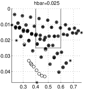
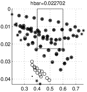
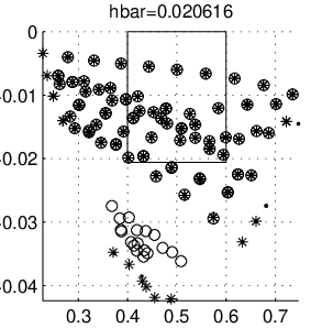
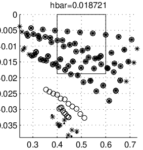
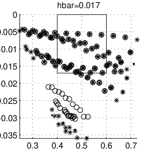
As an illustration of complex scaling, Figures 14 - 18 contain resonances for and . Eigenvalues of for different values of are marked by different styles of points, and the box has depth and width , with and . These plots may seem somewhat empty because only those eigenvalues of in regions of interest were computed. Notice the cluster of eigenvalues near the bottom edge of the plots: These are not resonances because they vary under perturbations in . Instead, they belong to an approximation of the (scaled) continuous spectrum.


6.2 Trapped Set Dimension

| 1.4 | 1.3092 | 1.2885 | 1.261 |
| 1.45 | 1.3084 | 1.2834 | 1.2558 |
| 1.5 | 1.3037 | 1.2829 | 1.2497 |
| 1.55 | 1.3007 | 1.2773 | 1.2521 |
| 1.6 | 1.2986 | 1.2725 | 1.2511 |
| 1.65 | 1.2912 | 1.2694 | 1.2488 |
| 1.7 | 1.2893 | 1.2636 | 1.2524 |
For comparison, is plotted as a function of in Figure 22. The figure contains curves corresponding to different energies : The top curve corresponds to , the middle curve , and the bottom curve . It also contains curves corresponding to different program parameters, to test the numerical convergence of dimension estimates. These curves were computed with , , and recursion depth (corresponding to symmetric sequences of length ); the caption contains the values of and for each curve. For reference, Table 1 contains the dimension estimates shown in the graph. It is important to note that, while the dimension does depend on and , it only does so weakly: Relative to its value, is very roughly constant across the range of and computed here.
6.3 Discussion
| slope | relative error | ||
|---|---|---|---|
| 1.4 | 1.2475 | 1.2885 | 0.032888 |
| 1.45 | 1.3433 | 1.2834 | 0.044645 |
| 1.5 | 1.2822 | 1.2829 | 0.00052244 |
| 1.55 | 1.327 | 1.2773 | 0.037472 |
| 1.6 | 1.3055 | 1.2725 | 0.025256 |
| 1.65 | 1.2304 | 1.2694 | 0.031756 |
| 1.7 | 1.2431 | 1.2636 | 0.016509 |

Table 2 contains a comparison of (for ) as a function of , versus the scaling exponents from Figure 21. Figure 23 is a graphical representation of similar information. This figure shows that even though the scaling curve in Figure 21 is noisy, its trend nevertheless agrees with the conjecture. Furthermore, the relative size of the fluctuations is small. At the present time, the source of the fluctuation is not known, but it is possibly due to the fact that the range of explored here is simply too large to exhibit the asymptotic behavior clearly.1717 17 But see Footnote 8.
Figures 24 - 30 contain plots of versus , for various values of . Along with the numerical data, the least-squares linear fit and the scaling law predicted by the conjecture are also plotted.1818 18 The conjecture only supplies the exponents for power laws, not the constant factors. In the context of these logarithmic plots, this means the conjecture gives us only the slopes, not the vertical shifts. It was thus necessary to compute an -intercept for each “prediction” curve (for the scaling law predicted by the conjecture) using least squares. In contrast with Figure 23, these show clear agrement between the asymptotic distribution of resonances and the scaling exponent predicted by the conjecture.


6.4 Double Gaussian Scattering
Finally, we compute resonances for the double gaussian model (setting in (6). This case is interesting for two reasons: First, there exist rigorous results [13, 21] against which we can check the correctness of our results. Second, it helps determine the validity of semiclassical arguments for the values of used in computing resonances for the triple gaussian model.
The resonances are shown in Figures 31 - 37: In these plots, and ranges from to . One can observe apparent pseudospectral effects in the first few figures [30, 36]; this is most likely because the scaling angle used here is twice as large as suggested in Section 4.1, to exhibit the structure of resonances farther away from the real axis.


To compare this information with known results [13, 21], we need some definitions: For a given energy , define by
| (48) |
where the limits of integration are
| (49) |
Let denote the larger (in absolute value) eigenvalue of ; is the Lyapunov exponent of , and is easy to compute numerically in this case. Note that for two-bump scattering, each energy determines a unique periodic trapped trajectory, and is the classical action computed along that trajectory.
Since these expressions are analytic, they have continuations to a neighborhood of the real line — becomes a contour integral. In [13], it was shown that any resonance must satisfy
| (50) |
where and are nonnegative integers. (The in comes from the Maslov index associated with the classical turning points.) This suggests that we define the map , where
| (51) |
and
| (52) |
should map resonances to points on the square integer lattice, and this is indeed the case: Figures 38 - 44 contain images of resonances under , with circles marking the nearest lattice points. The agreement is quite good, in view of the fact that we neglected terms of order in Equation (50).


7 Conclusions
Using standard numerical techniqes, one can compute a sufficiently large number of resonances for the triple gaussian system to verify their asymptotic distribution in the semiclassical limit . This, combined with effective estimates of the fractal dimension of the classical trapped set, gives strong evidence that the number of resonances in a box , for sufficiently small and ,
| (53) |
as one can see in Figure 23 and Table 2. Furthermore, the same techniques, when applied to double gaussian scattering, produce results which agree with rigorous semiclassical results. This supports the correctness of our algorithms and the validity of semiclassical arguments for the range of explored in the triple gaussian model. The computation also hints at more detailed structures in the distribution of resonances: In Figures 14 - 18, one can clearly see gaps and strips in the distribution of resonances. A complete understanding of this structure requires further investigation.
While we do not have rigorous error bounds for the dimension estimates, the numerical results are convincing. It seems, then, that the primary cause for our failure to observe the conjecture in a “clean” way is partly due to the size of : If one could study resonances at much smaller values of , the asymptotics may become more clear.
8 Acknowledgments
Thanks to J. Demmel and B. Parlett for crucial help with matrix computations, and to X. S. Li and C. Yang for ARPACK help. Thanks are also due to R. Littlejohn and M. Cargo for their help with bases and matrix elements, and to F. Bonetto for suggesting a practical method for computing fractal dimensions. Many thanks to Z. Bai, W. H. Miller, and J. Harrison for helpful conversations, and to the Mathematics Department at Lawrence Berkeley National Laboratory for computational resources. Finally, the author owes much to M. Zworski for inspiring most of this work.
KL was supported by the Fannie and John Hertz Foundation.
References
- [1] J. Aguilar, J. M. Combes. “A class of analytic perturbations for one body Schrödinger Hamiltonians,” Comm. Math. Phys. 22 (1971), 269-279.
- [2] E. Anderson, Z. Bai, C. Bischof, et al. LAPACK User’s Guide, Third Edition. SIAM, 1999.
- [3] E. Balslev, J. M. Combes. “Spectral properties of many-body Schrödingeroperators with dilation analytic interactions,” Comm. Math. Phys. 22 (1971), 280-294.
- [4] R. Barrett, M. Berry, T. F. Chan, et al. Templates for the Solution of Linear Systems: Building Blocks for Iterative Methods. SIAM, 1994.
- [5] H. A. Bethe, E. E. Salpeter. Quantum Mechanics of One- and Two-Electron Atoms. Plenum Publications, c1977.
- [6] M. J. Davis, E. J. Heller. “Semiclassical Gaussian basis set method for molecular vibrational wave functions,” J. Chem. Phys. 71 (1979), no. 8, 3383.
- [7] M. Dimassi, J. Sjöstrand. Spectral Asymptotics in the Semi-Classical Limit. Cambridge University Press, 1999.
- [8] K. J. Falconer. Fractal Geometry: Mathematical Foundations and Applications. John Wiley and Sons, 1990.
- [9] P. Gaspard, S. A. Rice. “Scattering from a classically chaotic repellor,” J. Chem. Phys. 90 (1989), 2225.
- [10] P. Gaspard, S. A. Rice. “Semiclassical quantization of the scattering from a classically chaotic repellor,” J. Chem. Phys. 90 (1989), 2242.
- [11] P. Gaspard, S. A. Rice. “Exact quantization of the scattering from a classically chaotic repellor,” J. Chem. Phys. 90 (1989), 2255.
- [12] P. Gaspard. Chaos, Scattering, and Statistical Mechanics. Cambridge University Press, 1998.
- [13] C. Gérard, J. Sjöstrand. “Semiclassical resonances generated by a closed trajectory of hyperbolic type,” Comm. Math. Phys. 108 (1987), no. 3, 391-421.
- [14] L. Guillopé, M. Zworski. “Wave trace for Riemann surfaces,” Geom. and Func. Anal. 6 (1999), 1156-1168.
- [15] I. P. Hamilton, J. C. Light. “On distributed Gaussian bases for simple model multidimensional vibrational problems,” J. Chem. Phys. 84 (1986), no. 1, 306.
- [16] M. Kac. “Can one hear the shape of a drum?” Amer. Math. Monthly 73 (1966), no. 4, 1-23.
- [17] A. Knauf. “The -Centre Problem of Celestial Mechanics” (2000), preprint.
- [18] A. Lahmar-Benbernou, A. Martinez. “On Helffer-Sjöstrand’s theory of resonances,” preprint.
- [19] R. B. Lehoucq, D. C. Sorensen, C. Yang. ARPACK User’s Guide: Solution of Large-Scale Eigenvalue Problems with Implicitly Restarted Arnoldi Methods. SIAM, 1998.
- [20] J. C. Light, I. P. Hamilton, J. V. Lill. “Generalized discrete variable approximation in quantum mechanics,” J. Chem. Phys. 82 (1985), 1400-1409.
- [21] W. H. Miller. “Classical-limit Green’s function (fixed-energy propagator) and classical quantization of nonseparable systems,” J. Chem. Phys. 56 (1972), no. 1, 38-45.
- [22] W. H. Miller. “Tunneling and state specificity in unimolecular reactions,” Chem. Rev. 87 (1987), 19-27.
- [23] Ya. B. Pesin. Dimension Theory in Dynamical Systems: Contemporary Views and Applications. Univ. of Chicago Press, 1997.
- [24] T. N. Rescigno, M. Baertschy, W. A. Isaacs, C. W. McCurdy. “Collisional breakup in a quantum system of three charged particles,” Science 286 (1999), 2474-2479.
- [25] W. McC. Siebert. Circuits, Signals, and Systems. MIT Press, 1986.
- [26] B. Simon. “The definition of molecular resonance curves by the method of exterior complex scaling,” Phys. Lett. A 71 (1979), 211-214.
- [27] J. Sjöstrand. “Geometric bounds on the density of resonances for semi-classical problems,” Duke Math. J. 60 (1990), 1-57.
- [28] J. Sjöstrand, M. Zworski. “Complex scaling and the distribution of scattering poles,” Jour. Amer. Math. Soc. 4 (1991), 729-769.
- [29] G. J. Sussman, J. Wisdom, M. E. Mayer. Structure and Interpretation of Classical Mechanics. MIT Press, 2001.
- [30] L. N. Trefethen. “Pseudospectra of Linear Operators,” SIAM Review 39 (1989), no. 3, 383-406.
- [31] B. A. Waite, W. H. Miller. “Model studies of mode specificity in unimolecular reaction dynamics,” J. Chem. Phys. 73 (1980), no. 8, 3713-3721.
- [32] B. A. Waite, W. H. Miller. “Mode specificity in unimolecular reaction dynamics: the Hénon-Heiles potential energy surface,” J. Chem. Phys. 74 (1981), no. 7, 3910-3915.
- [33] M. Wei, G. Majda, W. Strauss. “Numerical Computation of the Scattering Frequencies for Acoustic Wave Equations,” J. Comp. Phys. 75 (1988), no. 2, 345-358.
- [34] A. Wirzba. “Quantum mechanics and semiclassics of hyperbolic -disk scattering systems,” Phys. Rep. 309 (1999), no. 1-2.
- [35] M. Zworski, “Dimension of the limit set and the density of resonances for convex co-compact hyperbolic surfaces,” Invent. Math. 136 (1999), 353-409.
- [36] M. Zworski, “Numerical linear algebra and solvability of partial differential equations” (2001), preprint.
- [37] M. Zworski. “Resonances in Geometry and Physics,” Notices of the AMS, March 1999, 319-328.