Hexagonal circle patterns and integrable systems:
Patterns with the multi-ratio property
and Lax equations on the regular triangular lattice

A.I. Bobenko Note: E–mail: bobenko@math.tu-berlin.de T. Hoffmann Note: E–mail: timh@sfb288.math.tu-berlin.de Yu.B. Suris Note: E–mail: suris@sfb288.math.tu-berlin.de

Fachbereich Mathematik, Technische Universität Berlin, Str. 17 Juni 136, 10623 Berlin, Germany

Abstract

Hexagonal circle patterns are introduced, and a subclass thereof is studied in detail. It is characterized by the following property: For every circle the multi-ratio of its six intersection points with neighboring circles is equal to $-1$ . The relation of such patterns with an integrable system on the regular triangular lattice is established. A kind of a Bäcklund transformation for circle patterns is studied. Further, a class of isomonodromic solutions of the aforementioned integrable system is introduced, including circle patterns analogons to the analytic functions $z^{\alpha}$ and $\log z$ .

1 Introduction

The theory of circle packings and, more generally, of circle patterns enjoys in recent years a fast development and a growing interest of specialists in complex analysis. The origin of this interest was connected with the Thurston’s idea about approximating the Riemann mapping by circle packings, see [T1], [RS]. Since then the theory bifurcated to several subareas. One of them concentrates around the uniformization theorem of Koebe–Andreev–Thurston, and is dealing with circle packing realizations of cell complexes of a prescribed combinatorics, rigidity properties, constructing hyperbolic 3-manifolds, etc [T2], [MR], [BS], [H].

Another one is mainly dealing with approximation problems, and in this context it is advantageous to stick from the beginning with fixed regular combinatorics. The most popular are hexagonal packings, for which the $C^{\infty}$ convergence to the Riemann mapping was established by He and Schramm [HS]. Similar results are available also for circle patterns with the combinatorics of the square grid introduced by Schramm [S]. It is also the context of regular patterns (more precisely, the two just mentioned classes thereof) where some progress was achieved in constructing discrete analogs of analytic functions (Doyle’s spiralling hexagon packings [BDS] and their generalizations including the discrete analog of a quotient of Airy functions [BH], discrete analogs of ${\rm exp}(z)$ and ${\rm erf}(z)$ for the square grid circle patterns [S], discrete versions of $z^{\alpha}$ and $\log z$ for the same class of circle patterns [BP], [AB]). And it is again the context of regular patterns where the theory comes into interplay with the theory of integrable systems. Strictly speaking, only one instance of such an interplay is well–established up to now: namely, Schramm’s equation describing the square grid circle packings in terms of Möbius invariants turns out to coincide with the stationary Hirota’s equation, known to be integrable, see [BP], [Z]. It should be said that, generally, the subject of discrete integrable systems on lattices different from ${{Z}}^{n}$ is underdeveloped at present. The list of relevant publications is almost exhausted by [ND], [NS], [KN], [A], [OP].

The present paper contributes to several of the above mentioned issues: we introduce a new interesting class of circle patterns, and relate them to integrable systems. Besides, for this class we construct, in parallel to [BP], [AB], the analogs of the analytic functions $z^{\alpha}$ , $\log z$ .

This class is constituted by hexagonal circle patterns, or, in other words, by circle patterns with the combinatorics of the regular hexagonal lattice (the honeycomb lattice). This means that each elementary hexagon of the honeycomb lattice corresponds to a circle, and each common vertex of two hexagons corresponds to an intersection point of the corresponding circles. In particular, each circle carries six intersection points with six neighboring circles. Since at each vertex of the honeycomb lattice there meet three elementary hexagons, there follows that at each intersection point there meet three circles.

This class of hexagonal circle patterns is still too wide to be manageable, but it includes several very interesting subclasses, leading to integrable systems. For example, one can prescribe intersection angles of the circles. This situation will be considered in a subsequent publication. In the present one we consider the following requirement: the six intersection points on each circle have the multi-ratio equal to $-1$ , where the multi–ratio is a natural generalization of the notion of a cross-ratio of four points on a plane.

We show that, adding to the intersection points of the circles their centers, one embeds hexagonal circle patterns with the multi-ratio property into an integrable system on the regular triangular lattice. Each solution of this latter system describes a peculiar geometrical construction: it consists of three triangulations of the plane, such that the corresponding elementary triangles in all three tilings are similar. Moreover, given one such tiling, one can reconstruct the other two almost uniquely (up to an affine transformation). If one of the tilings comes from the hexagonal circle pattern, so do the other two. This results are contained in Sect. 2, 4. In the intermediate Sect. 3 we discuss a general notion of integrable systems on graphs as flat connections with the values in loop groups. It should be noticed that closely related integrable equations (albeit on the standard grid ${{Z}}^{2}$ ) were previously introduced by Nijhoff [N] in a totally different context (discrete Bussinesq equation), see also similar results in [BK]. However, these results did not go beyond writing down the equations: geometrical structures behind the equations were not discussed in these papers.

Having included hexagonal circle patterns with the multi-ratio property into the framework of the theory of integrable systems, we get an opportunity of applying the immense machinery of the latter to studying the properties of the former. This is illustrated in Sect. 5, 6, where we introduce and study some isomonodromic solutions of our integrable system on the triangular lattice, as well as the corresponding circle patterns. Finally, in Sect. 7 we define a subclass of these “isomonodromic circle patterns” which are natural discrete versions of the analytic functions $z^{\alpha}$ , $\log z$ . The results of Sect. 5–7 constitute an extension to the present, somewhat more intricate, situation of the similar constructions for Schramm’s circle patterns with the combinatorics of the square grid [AB].

2 Hexagonal circle patterns

Refer to caption — Figure 1: The regular triangular lattice with its hexagonal sublattices.

First of all we define the regular triangular lattice ${\cal T}{\cal L}$ as the cell complex whose vertices are

V({\cal T}{\cal L})=\Big\{{{z}}=k+\ell\omega+m\omega^{2}:\;k,\ell,m\in{{Z}}\Big\},\quad{\rm where}\quad\omega=\exp(2\pi i/3),

(2.1)

whose edges are all non–ordered pairs

E({\cal T}{\cal L})=\Big\{[{{z}}_{1},{{z}}_{2}]:\;{{z}}_{1},{{z}}_{2}\in V({\cal T}{\cal L}),\;|{{z}}_{1}-{{z}}_{2}|=1\Big\},

(2.2)

and whose 2-cells are all regular triangles with the vertices in $V({\cal T}{\cal L})$ and the edges in $E({\cal T}{\cal L})$ . We shall use triples $(k,\ell,m)\in{{Z}}^{3}$ as coordinates of the vertices of the regular triangular lattice, identifying two such triples iff they differ by the vector $(n,n,n)$ with $n\in{{Z}}$ . We call two points ${{z}}_{1},{{z}}_{2}$ neighbors in ${\cal T}{\cal L}$ , iff $[{{z}}_{1},{{z}}_{2}]\in E({\cal T}{\cal L})$ .

To the complex ${\cal T}{\cal L}$ there correspond three regular hexagonal sublattices ${\cal H}{\cal L}_{j}$ , $j=0,1,2$ . Each ${\cal H}{\cal L}_{j}$ is the cell complex whose vertices are

V({\cal H}{\cal L}_{j})=\Big\{{{z}}=k+\ell\omega+m\omega^{2}:\;k,\ell,m\in{{Z}},\;k+\ell+m\not\equiv j\!\!\pmod{3}\Big\},

(2.3)

whose edges are

E({\cal H}{\cal L}_{j})=\Big\{[{{z}}_{1},{{z}}_{2}]:\;{{z}}_{1},{{z}}_{2}\in V({\cal H}{\cal L}_{j}),\;|{{z}}_{1}-{{z}}_{2}|=1\Big\},

(2.4)

and whose 2-cells are all regular hexagons with the vertices in $V({\cal H}{\cal L}_{j})$ and the edges in $E({\cal H}{\cal L}_{j})$ . Again, we call two points ${{z}}_{1},{{z}}_{2}$ neighbors in ${\cal H}{\cal L}_{j}$ , iff $[{{z}}_{1},{{z}}_{2}]\in E({\cal H}{\cal L}_{j})$ . Obviously, every point in $V({\cal H}{\cal L}_{j})$ has three neighbors in ${\cal H}{\cal L}_{j}$ , as well as three neighbors in ${\cal T}{\cal L}$ which do not belong to $V({\cal H}{\cal L}_{j})$ . The centers of 2-cells of ${\cal H}{\cal L}_{j}$ are exactly the points of $V({\cal T}{\cal L})\setminus V({\cal H}{\cal L}_{j})$ , i.e. the points ${{z}}^{\prime}=k+\ell\omega+m\omega^{2}$ with $k+\ell+m\equiv j\!\!\pmod{3}$ .

In the following definition we consider only ${\cal H}{\cal L}_{0}$ , since, clearly, ${\cal H}{\cal L}_{1}$ and ${\cal H}{\cal L}_{2}$ are obtained from ${\cal H}{\cal L}_{0}$ via shifting all the corresponding objects by $\omega$ , resp. by $\omega^{2}$ .

Definition 1

We say that a map $w:V({\cal H}{\cal L}_{0})\mapsto\hat{{C}}$ defines a hexagonal circle pattern, if the following condition is satisfied:

•

Let

${{z}}_{k}={{z}}^{\prime}+\varepsilon^{k}\in V({\cal H}{\cal L}_{0}),\quad k=1,2,\ldots,6,\quad where\quad\varepsilon=\exp(\pi i/3),$

be the vertices of any elementary hexagon in ${\cal H}{\cal L}_{0}$ with the center ${{z}}^{\prime}\in V({\cal T}{\cal L})\setminus V({\cal H}{\cal L}_{0})$ . Then the points $w({{z}}_{1}),w({{z}}_{2}),\ldots,w({{z}}_{6})\in\hat{{C}}$ lie on a circle, and their circular order is just the listed one. We denote the circle through the points $w({{z}}_{1}),w({{z}}_{2}),\ldots,w({{z}}_{6})$ by $C({{z}}^{\prime})$ , thus putting it into a correspondence with the center ${{z}}^{\prime}$ of the elementary hexagon above.

As a consequence of this condition, we see that if two elementary hexagons of ${\cal H}{\cal L}_{0}$ with the centers in ${{z}}^{\prime},{{z}}^{\prime\prime}\in V({\cal T}{\cal L})\setminus V({\cal H}{\cal L}_{0})$ have a common edge $[{{z}}_{1},{{z}}_{2}]\in E({\cal H}{\cal L}_{0})$ , then the circles $C({{z}}^{\prime})$ and $C({{z}}^{\prime\prime})$ intersect in the points $w({{z}}_{1})$ , $w({{z}}_{2})$ . Similarly, if three elementary hexagons of ${\cal H}{\cal L}_{0}$ with the centers in ${{z}}^{\prime},{{z}}^{\prime\prime},{{z}}^{\prime\prime\prime}\in V({\cal T}{\cal L})\setminus V({\cal H}{\cal L}_{0})$ meet in one point ${{z}}_{0}\in V({\cal H}{\cal L}_{0})$ , then the circles $C({{z}}^{\prime})$ , $C({{z}}^{\prime\prime})$ and $C({{z}}^{\prime\prime\prime})$ also have a common intersection point $w({{z}}_{0})$ . (Note that in every point ${{z}}_{0}\in V({\cal H}{\cal L}_{0})$ there meet three distinct elementary hexagons of ${\cal H}{\cal L}_{0}$ ).

Remark. Sometimes it will be convenient to consider circle patterns defined not on the whole of ${\cal H}{\cal L}_{0}$ , but rather on some connected subgraph of the regular hexagonal lattice.

We shall study in this paper a subclass of hexagonal circle patterns satisfying an additional condition. We need the following generalization of the notion of cross-ratio.

Definition 2

Given a $(2p)$ -tuple $(w_{1},w_{2},\ldots,w_{2p})\in{{C}}^{2p}$ of complex numbers, their multi-ratio is the following number:

M(w_{1},w_{2},\ldots,w_{2p})=\frac{\prod_{j=1}^{p}(w_{2j-1}-w_{2j})}{\prod_{j=1}^{p}(w_{2j}-w_{2j+1})},

(2.5)

where it is agreed that $w_{2p+1}=w_{1}$ .

In particular,

M(w_{1},w_{2},w_{3},w_{4})=\frac{(w_{1}-w_{2})(w_{3}-w_{4})}{(w_{2}-w_{3})(w_{4}-w_{1})}

is the usual cross-ratio, while in the present paper we shall be mainly dealing with

M(w_{1},w_{2},\ldots,w_{6})=\frac{(w_{1}-w_{2})(w_{3}-w_{4})(w_{5}-w_{6})}{(w_{2}-w_{3})(w_{4}-w_{5})(w_{6}-w_{1})}.

The following two obvious properties of the multi-ratio will be important for us:

(i)

The multi-ratio $M(w_{1},w_{2},\ldots,w_{2p})$ is invariant with respect to the action of an arbitrary Möbius transformation $w\mapsto(aw+b)/(cw+d)$ on all of its arguments.
(ii)

The multi-ratio $M(w_{1},w_{2},\ldots,w_{2p})$ is a Möbius transformation with respect to each one of its arguments.

We shall need also the following, slightly less obvious, property:

(iii)

If the points $w_{1},w_{2},\ldots,w_{2p-1}$ lie on a circle $C\subset\hat{{C}}$ , and the multi-ratio $M(w_{1},w_{2},\ldots,w_{2p})$ is real, then also $w_{2p}\in C$ .

Definition 3

We say that a map $w:V({\cal H}{\cal L}_{0})\mapsto\hat{{C}}$ defines a hexagonal circle pattern with $\boldsymbol{M}\boldsymbol{R}\boldsymbol{=}\boldsymbol{-}\boldsymbol{1}$ , if in addition to the condition of Definition 1 the following one is satisfied:

•

For any elementary hexagon in ${\cal H}{\cal L}_{0}$ with the vertices ${{z}}_{1},{{z}}_{2},\ldots,{{z}}_{6}\in V({\cal H}{\cal L}_{0})$ (listed counterclockwise), the multi-ratio

$M(w_{1},w_{2},\ldots,w_{6})=-1,$ (2.6)

where $w_{k}=w({{z}}_{k})$ .

Geometrically the condition (2.6) means that, first, the lengths of the sides of the hexagon with the vertices $w_{1}w_{2}\ldots w_{6}$ satisfy the condition

|w_{1}-w_{2}|\cdot|w_{3}-w_{4}|\cdot|w_{5}-w_{6}|=|w_{2}-w_{3}|\cdot|w_{4}-w_{5}|\cdot|w_{6}-w_{1}|,

and, second, that the sum of the angles of the hexagon at the vertices $w_{1}$ , $w_{3}$ , and $w_{5}$ is equal to $2\pi\!\!\pmod{2\pi}$ , as well as the sum of the angles at the vertices $w_{2}$ , $w_{4}$ , and $w_{6}$ . Notice that if a hexagon is inscribed in a circle and satisfies (2.6), then it is conformally symmetric, i.e. there exists a Möbius transformation mapping it onto a centrally symmetric hexagon. Notice also that the regular hexagons satisfy this condition.

To demonstrate quickly the existence of hexagonal circle patterns with $MR=-1$ we give their construction via solving a suitable Cauchy problem.

Lemma 4

Consider a row of elementary hexagons of ${\cal H}{\cal L}_{0}$ running from the north–west to the south-east, with the centers in the points ${{z}}^{\prime}_{k}=k-k\omega$ . Let the map $w$ be defined in five vertices of each hexagon – in all except ${{z}}^{\prime}_{k}+\varepsilon$ . Suppose that the five points $w({{z}}^{\prime}_{k}+\varepsilon^{j})$ , $j=2,3,\ldots,6$ , lie on the circles $C({{z}}^{\prime}_{k})$ . These data determine uniquely a map $w:V({\cal H}{\cal L}_{0})\mapsto\hat{{C}}$ yielding a hexagonal circle pattern with $MR=-1$ on the whole lattice.

Proof. Equation (2.6) determines the points $w({{z}}^{\prime}_{k}+\varepsilon)$ , which, according to the property above, lie also on $C({{z}}^{\prime}_{k})$ . Now for every hexagon of the parallel row next to north–east, with the centers in the points ${{z}}^{\prime\prime}_{k}={{z}}^{\prime}_{k}+1+\varepsilon=(k+2)-(k-1)\omega$ , we know the value of the map $w$ in three vertices, namely in

{{z}}^{\prime\prime}_{k}+\varepsilon^{4}={{z}}^{\prime}_{k}+1={{z}}^{\prime}_{k+1}+\varepsilon^{2},\quad{{z}}^{\prime\prime}_{k}+\varepsilon^{3}={{z}}^{\prime}_{k}+\varepsilon,\quad{{z}}^{\prime\prime}_{k}+\varepsilon^{5}={{z}}^{\prime}_{k+1}+\varepsilon^{2}.

This uniquely defines the circle $C({{z}}^{\prime\prime}_{k})$ , as the only circle through three points $w({{z}}^{\prime\prime}_{k}+\varepsilon^{3})$ , $w({{z}}^{\prime\prime}_{k}+\varepsilon^{4})$ and $w({{z}}^{\prime\prime}_{k}+\varepsilon^{5})$ . The intersection points of these circles of the second row give us the values of the map $w$ in the points ${{z}}^{\prime\prime}_{k}+\varepsilon^{2}$ and ${{z}}^{\prime\prime}_{k}+\varepsilon^{6}$ . Namely, $w({{z}}^{\prime\prime}_{k}+\varepsilon^{2})$ is the intersection point of $C({{z}}^{\prime\prime}_{k})$ with $C({{z}}^{\prime\prime}_{k-1})$ , different from $w({{z}}^{\prime\prime}_{k}+\varepsilon^{3})$ , and $w({{z}}^{\prime\prime}_{k}+\varepsilon^{6})$ is the intersection point of $C({{z}}^{\prime\prime}_{k})$ with $C({{z}}^{\prime\prime}_{k+1})$ , different from $w({{z}}^{\prime\prime}_{k}+\varepsilon^{5})$ . Therefore we get the values of the map $w$ in five vertices of each hexagon of the next parallel row – in all except ${{z}}^{\prime\prime}_{k}+\varepsilon$ . The induction allows to continue the construction ad infinitum.

Now we show that, adding the centers of the circles of a hexagonal pattern with $MR=-1$ to their intersection points, we come to a new interesting notion.

Theorem 5

Let the map $w:V({\cal H}{\cal L}_{0})\mapsto\hat{{C}}$ define a hexagonal circle pattern with $MR=-1$ . Extend $w$ to the points of $V({\cal T}{\cal L})\setminus V({\cal H}{\cal L}_{0})$ by the following rule. Fix some point $P_{\infty}\in\hat{{C}}$ . Let ${{z}}^{\prime}$ be a center of an elementary hexagon of ${\cal H}{\cal L}_{0}$ . Set $w({{z}}^{\prime})$ to be the reflection of the point $P_{\infty}$ in the circle $C({{z}}^{\prime})$ . Then the condition (2.6) holds also for $w_{k}=w({{z}}_{k})$ in the case when the points ${{z}}_{1},{{z}}_{2},\ldots,{{z}}_{6}$ are the vertices of any elementary hexagon of the two complementary hexagonal sublattices ${\cal H}{\cal L}_{1}$ and ${\cal H}{\cal L}_{2}$ .

Figure 2: An elementary hexagon with its center point sent to

\infty

Proof. Consider the situation corresponding to an elementary hexagon of the sublattice ${\cal H}{\cal L}_{1}$ or ${\cal H}{\cal L}_{2}$ (see Fig. 2). The point $w_{0}$ is the intersection point of the three circles $C({{z}}_{1})$ , $C({{z}}_{3})$ , and $C({{z}}_{5})$ , the points $w_{1}$ , $w_{3}$ , and $w_{5}$ are obtained by reflection of $P_{\infty}$ in the corresponding circles, and the points $w_{2}$ , $w_{4}$ , and $w_{6}$ are the pairwise intersection points of these circles different from $w_{0}$ . To simplify the geometry behind this situation, perform a Möbius transformation sending $w_{0}$ to infinity. Then the circles $C({{z}}_{1})$ , $C({{z}}_{3})$ , and $C({{z}}_{5})$ become straight lines, and the points $w_{1}$ , $w_{3}$ , $w_{5}$ are the reflections of $P_{\infty}$ in these lines (see Fig. 2; for definiteness we suppose here that the Möbius image of $P_{\infty}$ lies in the interior of the triangle formed by these straight lines). By construction, one gets:

|w_{2}-w_{1}|=|w_{2}-w_{3}|,\quad|w_{4}-w_{3}|=|w_{4}-w_{5}|,\quad|w_{6}-w_{5}|=|w_{6}-w_{1}|;

the angles by the vertices $w_{2}$ , $w_{4}$ , $w_{6}$ are equal to $2(\alpha_{1}+\alpha_{2})$ , $2(\beta_{1}+\beta_{2})$ , $2(\gamma_{1}+\gamma_{2})$ , respectively, so that their sum is equal to

2(\alpha_{1}+\alpha_{2}+\beta_{1}+\beta_{2}+\gamma_{1}+\gamma_{2})=2\pi;

the angles by the vertices $w_{1}$ , $w_{3}$ , $w_{5}$ are equal to $\pi-(\alpha_{1}+\gamma_{2})$ , $\pi-(\beta_{1}+\alpha_{2})$ , $\pi-(\gamma_{1}+\beta_{2})$ , respectively, so that their sum is equal to

3\pi-(\alpha_{1}+\alpha_{2}+\beta_{1}+\beta_{2}+\gamma_{1}+\gamma_{2})=2\pi.

This proves that the hexagon under consideration satisfies (2.6).

A particular case of the construction of Theorem 5 is when $P_{\infty}=\infty$ , so that the map $w$ is extended by the centers of the corresponding circles. In any case, this theorem suggests to consider the class of maps described in the following definition.

Definition 6

We say that the map $w:V({\cal T}{\cal L})\mapsto\hat{{C}}$ defines a triangular lattice with $\boldsymbol{M}\boldsymbol{R}\boldsymbol{=}\boldsymbol{-}\boldsymbol{1}$ , if the equation (2.6) holds for $w_{k}=w({{z}}_{k})$ , whenever the points ${{z}}_{1},{{z}}_{2},\ldots,{{z}}_{6}$ are the vertices (listed counterclockwise) of any elementary hexagon of any of the sublattices ${\cal H}{\cal L}_{j}$ $(j=0,1,2)$ .

In the next section we shall discuss an integrable system on the regular triangular lattice, each solution of which delivers, in a single construction, three different triangular lattices with $MR=-1$ . However, these three lattices are not independent: given such a lattice, the two associated ones can be constructed almost uniquely (up to an affine transformation $w\mapsto aw+b$ ). It will turn out that if the original lattice comes from a hexagonal circle pattern with $MR=-1$ , then the two associated ones do likewise.

3 Discrete flat connections on graphs

Let us describe a general construction of “integrable systems” on graphs which does not hang on the specific features of the regular triangular lattice. This notion includes the following ingredients:

•

An oriented graph ${\cal G}$ ; the set of its vertices will be denoted $V({\cal G})$ , the set of its edges will be denoted $E({\cal G})$ .
•

A loop group $G[\lambda]$ , whose elements are functions from ${{C}}$ into some group $G$ . The complex argument $\lambda$ of these functions is known in the theory of integrable systems as the “spectral parameter”.
•

A “wave function” $\Psi:V({\cal G})\mapsto G[\lambda]$ , defined on the vertices of ${\cal G}$ .
•

A collection of “transition matrices” $L:E({\cal G})\mapsto G[\lambda]$ defined on the edges of ${\cal G}$ .

It is supposed that for any oriented edge ${{e}}=({{z}}_{1},{{z}}_{2})\in E({\cal G})$ the values of the wave functions in its ends are connected via

\Psi({{z}}_{2},\lambda)=L({{e}},\lambda)\Psi({{z}}_{1},\lambda).

(3.1)

Therefore the following discrete zero curvature condition is supposed to be satisfied. Consider any closed contour consisting of a finite number of edges of ${\cal G}$ :

{{e}}_{1}=({{z}}_{1},{{z}}_{2}),\quad{{e}}_{2}=({{z}}_{2},{{z}}_{3}),\quad\ldots,\quad{{e}}_{p}=({{z}}_{p},{{z}}_{1}).

Then

L({{e}}_{p},\lambda)\cdots L({{e}}_{2},\lambda)L({{e}}_{1},\lambda)=I.

(3.2)

In particular, for any edge ${{e}}=({{z}}_{1},{{z}}_{2})$ , if ${{e}}^{-1}=({{z}}_{2},{{z}}_{1})$ , then

L({{e}}^{-1},\lambda)=\Big(L({{e}},\lambda)\Big)^{-1}.

(3.3)

Actually, in applications the matrices $L({{e}},\lambda)$ depend also on a point of some set $X$ (the “phase space” of an integrable system), so that some elements $x({{e}})\in X$ are attached to the edges ${{e}}$ of ${\cal G}$ . In this case the discrete zero curvature condition (3.2) becomes equivalent to the collection of equations relating the fields $x({{e}}_{1})$ , $\ldots$ , $x({{e}}_{p})$ attached to the edges of each closed contour. We say that this collection of equations admits a zero curvature representation.

For an arbitrary graph, the analytical consequences of the zero curvature representation for a given collection of equations are not clear. However, in case of regular lattices, like ${\cal T}{\cal L}$ , such representation may be used to determine conserved quantities for suitably defined Cauchy problems, as well as to apply powerful analytical methods for finding concrete solutions.

Remark. The above construction of integrable systems on graphs is not the only possible one. For example, in the construction by Adler [A] the fields are defined on the vertices of a planar graph, and the equations relate the fields on stars consisting of the edges incident to each single vertex, rather than the fields on closed contours. Examples are given by discrete time systems of the relativistic Toda type. In the corresponding zero curvature representation the wave functions $\Psi$ naturally live on 2-cells rather than on vertices. The transition matrices live on edges: the matrix $L({{e}},\lambda)$ corresponds to the transition across ${{e}}$ and depends on the fields sitting on two ends of ${{e}}$ .

4 An integrable system on the regular triangular lattice

We now introduce an orientation of the edges of the regular triangular lattice ${\cal T}{\cal L}$ . Namely, we declare as positively oriented all edges of the types

({{z}},{{z}}+1),\quad({{z}},{{z}}+\omega),\quad({{z}},{{z}}+\omega^{2}).

Correspondingly, all edges of the types

({{z}},{{z}}-1),\quad({{z}},{{z}}-\omega),\quad({{z}},{{z}}-\omega^{2})

are negatively oriented. Thus all elementary triangles become oriented. There are two types of elementary triangles: those “pointing upwards” $({{z}},{{z}}+\omega,{{z}}-1)$ are oriented counterclockwise, while those “pointing downwards” $({{z}},{{z}}+\omega^{2},{{z}}-1)$ are oriented clockwise.

4.1 Lax representation

The group $G[\lambda]$ we use in our construction is the twisted loop group over ${\rm SL}(3,{{C}})$ :

\Big\{L:{{C}}\mapsto{\rm SL}(3,{{C}})\Big|\;L(\omega\lambda)=\Omega L(\lambda)\Omega^{-1}\Big\},

(4.1)

where $\Omega={\rm diag}(1,\omega,\omega^{2})$ . The elements of $G[\lambda]$ we attach to every positively oriented edge of ${\cal T}{\cal L}$ are of the form

L(\lambda)=(1+\lambda^{3})^{-1/3}\left(\begin{array}[]{ccc}1&\lambda f&0\\ 0&1&\lambda g\\ \lambda h&0&1\end{array}\right),\quad fgh=1.

(4.2)

Hence, to each positively oriented edge we assign a triple of complex numbers $(f,g,h)\in{{C}}^{3}$ satisfying an additional condition $fgh=1$ . In other words, choosing $(f,g)$ (say) as the basic variables, we can assume that the “phase space” $X$ mentioned in the previous section, is ${{C}}_{*}\times{{C}}_{*}$ . The scalar factor $(1+\lambda^{3})^{-1/3}$ is not very essential and assures merely that $\det L(\lambda)=1$ .

It is obvious that the zero curvature condition (3.2) is fulfilled for every closed contour in ${\cal T}{\cal L}$ , if and only if it holds for all elementary triangles.

Theorem 7

Let ${{e}}_{1}$ , ${{e}}_{2}$ , ${{e}}_{3}$ be the consecutive positively oriented edges of an elementary triangle of ${\cal T}{\cal L}$ . Then the zero curvature condition

L({{e}}_{3},\lambda)L({{e}}_{2},\lambda)L({{e}}_{1},\lambda)=I

is equivalent to the following set of equations:

f_{1}+f_{2}+f_{3}=0,\qquad g_{1}+g_{2}+g_{3}=0,

(4.3)

and

f_{1}g_{1}=f_{3}g_{2}\quad\Leftrightarrow\quad f_{2}g_{2}=f_{1}g_{3}\quad\Leftrightarrow\quad f_{3}g_{3}=f_{2}g_{1},

(4.4)

with the understanding that $h_{k}=(f_{k}g_{k})^{-1}$ , $k=1,2,3$ .

Proof. An easy calculation shows that the matrix equation $L_{3}L_{2}L_{1}=I$ consists of the following nine scalar equations:

f_{1}+f_{2}+f_{3}=0,\qquad g_{1}+g_{2}+g_{3}=0,\qquad h_{1}+h_{2}+h_{3}=0,

(4.5)

f_{3}g_{2}h_{1}=1,\qquad g_{3}h_{2}f_{1}=1,\qquad h_{3}f_{2}g_{1}=1,

(4.6)

f_{3}g_{2}+f_{3}g_{1}+f_{2}g_{1}=0,\qquad g_{3}h_{2}+g_{3}h_{1}+g_{2}h_{1}=0,\qquad h_{3}f_{2}+h_{3}f_{1}+h_{2}f_{1}=0.

(4.7)

It remains to isolate the independent ones among these nine equations. First of all, equations (4.7) are equivalent to (4.6), provided (4.5) and $f_{k}g_{k}h_{k}=1$ hold. For example:

f_{3}(g_{2}+g_{1})+f_{2}g_{1}=0\;\Leftrightarrow\;f_{3}g_{3}=f_{2}g_{1}\;\Leftrightarrow\;h_{3}f_{2}g_{1}=1.

Next, the conditions $f_{k}g_{k}h_{k}=1$ allow us to rewrite (4.6) as

f_{1}g_{1}=f_{3}g_{2},\qquad f_{2}g_{2}=f_{1}g_{3},\qquad f_{3}g_{3}=f_{2}g_{1}.

(4.8)

Further, all equations in (4.8) are equivalent provided (4.3) holds. For example:

f_{1}g_{1}=f_{3}g_{2}\;\Rightarrow\;(f_{2}+f_{3})g_{1}=f_{3}(g_{1}+g_{3})\;\Rightarrow f_{2}g_{1}=f_{3}g_{3}.

Finally, $h_{1}+h_{2}+h_{3}=0$ follows from (4.3), (4.4). Indeed,

$\displaystyle h_{1}+h_{2}$	$\displaystyle=$	$\displaystyle(f_{1}g_{1})^{-1}+(f_{2}g_{2})^{-1}=(f_{3}g_{2})^{-1}+(f_{2}g_{2})^{-1}$
	$\displaystyle=$	$\displaystyle(f_{2}g_{2})^{-1}(f_{2}+f_{3})f_{3}^{-1}=-(f_{2}g_{2})^{-1}f_{1}f_{3}^{-1}$
	$\displaystyle=$	$\displaystyle-(f_{1}g_{3})^{-1}f_{1}f_{3}^{-1}=-(f_{3}g_{3})^{-1}=-h_{3}.$

The theorem is proved. For want of a better name we shall call the system of equations (4.3), (4.4) the fgh–system.

The equations (4.5) may be interpreted in the following way: there exist functions $u,v,w:V({\cal T}{\cal L})\mapsto{{C}}$ such that for any positively oriented edge ${{e}}=({{z}}_{1},{{z}}_{2})$ there holds:

f({{e}})=u({{z}}_{2})-u({{z}}_{1}),\quad g({{e}})=v({{z}}_{2})-v({{z}}_{1}),\quad h({{e}})=w({{z}}_{2})-w({{z}}_{1}).

(4.9)

The function $u$ is determined by $f$ uniquely, up to an additive constant, and similarly for the functions $v$ , $w$ . Having introduced functions $u,v,w$ sitting in the vertices of ${\cal T}{\cal L}$ , we may reformulate the remaining equations (4.4) as follows: let ${{z}}_{1},{{z}}_{2},{{z}}_{3}$ be the consecutive vertices of a positively oriented elementary triangle, then

\frac{u({{z}}_{2})-u({{z}}_{1})}{u({{z}}_{3})-u({{z}}_{2})}=\frac{v({{z}}_{3})-v({{z}}_{2})}{v({{z}}_{1})-v({{z}}_{3})}.

(4.10)

The equations arising by cyclic permutations of indices $(1,2,3)\mapsto(2,3,1)$ are equivalent to this one due to (4.4). So, we have one equation pro elementary triangle ${{z}}_{1}{{z}}_{2}{{z}}_{3}$ . Its geometrical meaning is the following: the triangle $u({{z}}_{1})u({{z}}_{2})u({{z}}_{3})$ is similar to the triangle $v({{z}}_{2})v({{z}}_{3})v({{z}}_{1})$ (where the corresponding vertices are listed on the corresponding places). Of course, these two triangles are also similar to the third one, $w({{z}}_{3})w({{z}}_{1})w({{z}}_{2})$ .

4.2 Cauchy problem

We discuss now the Cauchy data which allow one to determine a solution of the $fgh$ –system. The key observation is the following.

Lemma 8

Given the values of two fields, say $u$ and $v$ , in three points ${{z}}_{0}$ , ${{z}}_{1}={{z}}_{0}+1$ and ${{z}}_{2}={{z}}_{0}+\omega$ , the equations of the $fgh$ –system determine uniquely the values of $u$ and $v$ in the point ${{z}}_{3}={{z}}_{0}+1+\omega$ :

u_{3}-u_{0}=(u_{1}-u_{0})\frac{v_{1}-v_{0}}{v_{1}-v_{2}}+(u_{2}-u_{0})\frac{v_{2}-v_{0}}{v_{2}-v_{1}},

(4.11)

v_{3}-v_{1}=(v_{1}-v_{0})\frac{u_{1}-u_{0}}{u_{0}-u_{3}}\quad\Leftrightarrow\quad v_{3}-v_{2}=(v_{2}-v_{0})\frac{u_{2}-u_{0}}{u_{0}-u_{3}}.

(4.12)

Proof. The formula (4.11) follows by eliminating $v_{3}$ from

\frac{u_{0}-u_{3}}{u_{1}-u_{0}}=\frac{v_{1}-v_{0}}{v_{3}-v_{1}},\qquad\frac{u_{0}-u_{3}}{u_{2}-u_{0}}=\frac{v_{2}-v_{0}}{v_{3}-v_{2}}.

(4.13)

These equations yield then (4.12).

This immediately yields the following statement.

Proposition 9

a)

The values of the fields $u$ and $v$ in the vertices of the zig–zag line running from the north–west to the south–east,

$\Big\{{{z}}=k+\ell\omega:k+\ell=0,1\Big\},$

uniquely determine the functions $u,v:V({\cal T}{\cal L})\mapsto{{C}}$ on the whole lattice.
b)

The values of the fields $u$ and $v$ on the two positive semi-axes,

$\Big\{{{z}}=k:k\geq 0\Big\}\cup\Big\{{{z}}=\ell\omega:\ell\geq 0\Big\},$

uniquely determine the functions $u,v$ on the whole sector

$\Big\{{{z}}=k+\ell\omega:k,\ell\geq 0\Big\}=\Big\{{{z}}\in V({\cal T}{\cal L}):0\leq{\rm\arg}({{z}})\leq 2\pi/3\Big\}.$

Proof follows by induction with the help of the formulas (4.11), (4.12).

4.3 Sym formula and related results

There holds the following result having many analogs in the differential geometry described by integrable systems (“Sym formula”, see, e.g., [BP]).

Proposition 10

Let $\Psi({{z}},\lambda)$ be the solution of (3.1) with the initial condition $\Psi({{z}}_{0},\lambda)=I$ for some ${{z}}_{0}\in V({\cal T}{\cal L})$ . Then the fields $u,v,w$ may be found as

\left.\frac{d\Psi}{d\lambda}\right|_{\lambda=0}=\left(\begin{array}[]{ccc}0&u&0\\ 0&0&v\\ w&0&0\end{array}\right).

(4.14)

Proof. Note, first of all, that from $\Psi({{z}}_{0},0)=I$ and $L({{e}},0)=I$ there follows that $\Psi({{z}},0)=I$ for all ${{z}}\in V({\cal T}{\cal L})$ . Consider an arbitrary positively oriented edge ${{e}}=({{z}}_{1},{{z}}_{2})$ . From (3.1) there follows:

\frac{d\Psi({{z}}_{2})}{d\lambda}-\frac{d\Psi({{z}}_{1})}{d\lambda}=\left(\frac{dL({{e}})}{d\lambda}\Psi({{z}}_{1})+L({{e}})\frac{d\Psi({{z}}_{1})}{d\lambda}\right)-\frac{d\Psi({{z}}_{1})}{d\lambda}

At $\lambda=0$ we find:

	$\displaystyle\left.\frac{d\Psi({{z}}_{2})}{d\lambda}\right\|_{\lambda=0}-\left.\frac{d\Psi({{z}}_{1})}{d\lambda}\right\|_{\lambda=0}=\left.\frac{dL({{e}})}{d\lambda}\right\|_{\lambda=0}=\left(\begin{array}[]{ccc}0&f({{e}})&0\\ 0&0&g({{e}})\\ h({{e}})&0&0\end{array}\right)$
		$\displaystyle=$	$\displaystyle\left(\begin{array}[]{ccc}0&u({{z}}_{2})-u({{z}}_{1})&0\\ 0&0&v({{z}}_{2})-v({{z}}_{1})\\ w({{z}}_{2})-w({{z}}_{1})&0&0\end{array}\right).$

This proves the Proposition.

Next terms of the power series expansion of the wave function $\Psi({{z}},\lambda)$ around $\lambda=0$ also deliver interesting and important results.

Proposition 11

Let $\Psi({{z}},\lambda)$ be the solution of (3.1) with the initial condition $\Psi({{z}}_{0},\lambda)=I$ for some ${{z}}_{0}\in V({\cal T}{\cal L})$ . Then

\frac{1}{2}\,\left.\frac{d^{2}\Psi}{d\lambda^{2}}\right|_{\lambda=0}=\left(\begin{array}[]{ccc}0&0&a\\ b&0&0\\ 0&c&0\end{array}\right),

(4.17)

where the function $a:V({\cal T}{\cal L})\mapsto{{C}}$ satisfies the difference equation

a({{z}}_{2})-a({{z}}_{1})=v({{z}}_{1})\Big(u({{z}}_{2})-u({{z}}_{1})\Big),

(4.18)

and similar equations hold for the functions $b,c:V({\cal T}{\cal L})\mapsto{{C}}$ (with the cyclic permutation $(u,v,w)\mapsto(w,u,v)$ ).

Proof. Proceeding as in the proof of Proposition 10, we have:

\frac{d^{2}\Psi({{z}}_{2})}{d\lambda^{2}}-\frac{d^{2}\Psi({{z}}_{1})}{d\lambda^{2}}=\left(\frac{d^{2}L({{e}})}{d\lambda^{2}}\Psi({{z}}_{1})+2\frac{dL({{e}})}{d\lambda}\frac{d\Psi({{z}}_{1})}{d\lambda}+L({{e}})\frac{d^{2}\Psi({{z}}_{1})}{d\lambda^{2}}\right)-\frac{d^{2}\Psi({{z}}_{1})}{d\lambda^{2}}

Taking into account that $d^{2}L({{e}})/d\lambda^{2}|_{\lambda=0}=0$ , we find at $\lambda=0$ :

	$\displaystyle\left.\frac{d^{2}\Psi({{z}}_{2})}{d\lambda^{2}}\right\|_{\lambda=0}-\left.\frac{d^{2}\Psi({{z}}_{1})}{d\lambda^{2}}\right\|_{\lambda=0}=2\left.\frac{dL({{e}})}{d\lambda}\right\|_{\lambda=0}\left.\frac{d\Psi({{z}}_{1})}{d\lambda}\right\|_{\lambda=0}=$
		$\displaystyle=$	$\displaystyle 2\left(\begin{array}[]{ccc}0&f({{e}})&0\\ 0&0&g({{e}})\\ h({{e}})&0&0\end{array}\right)\left(\begin{array}[]{ccc}0&u({{z}}_{1})&0\\ 0&0&v({{z}}_{1})\\ w({{z}}_{1})&0&0\end{array}\right).$

This implies the statement of the proposition.

Notice that it is à priori not obvious that the equation (4.18) admits a well–defined solution on $V({\cal T}{\cal L})$ , or, in other words, that its right–hand side defines a closed form on ${\cal T}{\cal L}$ . This fact might be proved by a direct calculation, based upon the equations of the $fgh$ –system, but the above argument gives a more conceptual and a much shorter proof.

Corollary 12

Under the conditions of Propositions 10,11, we have:

-\frac{1}{2}\,\left.\frac{d^{2}\Psi}{d\lambda^{2}}\right|_{\lambda=0}+\left(\frac{d\Psi}{d\lambda}\right)^{2}_{\lambda=0}=\left(\begin{array}[]{ccc}0&0&a^{\prime}\\ b^{\prime}&0&0\\ 0&c^{\prime}&0\end{array}\right),

(4.20)

where the function $a^{\prime}:V({\cal T}{\cal L})\mapsto{{C}}$ satisfies the difference equation

a^{\prime}({{z}}_{2})-a^{\prime}({{z}}_{1})=u({{z}}_{2})\Big(v({{z}}_{2})-v({{z}}_{1})\Big),

(4.21)

and similar equations hold for the functions $b^{\prime},c^{\prime}:V({\cal T}{\cal L})\mapsto{{C}}$ (with the cyclic permutation $(u,v,w)\mapsto(w,u,v)$ ).

Further examples of such exact forms may be obtained from the values of higher derivatives of the wave function $\Psi({{z}},\lambda)$ at $\lambda=0$ .

4.4 One–field equations

We discuss now the equations satisfied by the field $u$ alone, as well as by the field $v$ alone. In this point we make contact with the geometric considerations of Sect. 2.

Theorem 13

1.

Both maps $u,v:V({\cal T}{\cal L})\mapsto{{C}}$ define triangular lattices with $MR=-1$ . In other words, if ${{z}}_{1},{{z}}_{2},\ldots,{{z}}_{6}$ are the vertices (listed counterclockwise) of any elementary hexagon of any of the hexagonal sublattices ${\cal H}{\cal L}_{j}$ $(j=0,1,2)$ , and if $u_{k}=u({{z}}_{k})$ and $v_{k}=v({{z}}_{k})$ , then there hold both the equations

$M(u_{1},u_{2},\ldots,u_{6})=-1$ (4.22)

and

$M(v_{1},v_{2},\ldots,v_{6})=-1.$ (4.23)
2.

Given a triangular lattice $u:V({\cal T}{\cal L})\mapsto{{C}}$ with $MR=-1$ , there exists a unique, up to an affine transformation $v\mapsto av+b$ , function $v:V({\cal T}{\cal L})\mapsto{{C}}$ such that (4.10) are satisfied everywhere. This function also defines a triangular lattice with $MR=-1$ .
3.

Given a pair of complex–valued functions $(u,v)$ defined on $V({\cal T}{\cal L})$ and satisfying the equation (4.10) everywhere, there exists a unique, up to an affine transformation, function $w:V({\cal T}{\cal L})\mapsto{{C}}$ such that the pairs $(v,w)$ and $(w,u)$ satisfy the same equation. The function $w$ also defines a triangular lattice with $MR=-1$ .

Proof. 1. To prove the first statement, we proceed as follows. Let ${{z}}^{\prime}\in V({\cal T}{\cal L})$ , and let the vertices of an elementary hexagonal with the center in ${{z}}^{\prime}$ be enumerated as ${{z}}_{k}={{z}}^{\prime}+\varepsilon^{k}$ , $k=1,2,\ldots,6$ . Then the following elementary triangles are positively oriented: $({{z}}_{2k},{{z}}_{2k-1},{{z}}^{\prime})$ and $({{z}}_{2k},{{z}}_{2k+1},{{z}}^{\prime})$ for $k=1,2,3$ (with the agreement that ${{z}}_{7}={{z}}_{1}$ ). According to (4.10), we have:

\frac{u_{2k-1}-u_{2k}}{u^{\prime}-u_{2k-1}}=\frac{v^{\prime}-v_{2k-1}}{v_{2k}-v^{\prime}},\qquad\frac{u_{2k+1}-u_{2k}}{u^{\prime}-u_{2k+1}}=\frac{v^{\prime}-v_{2k+1}}{v_{2k}-v^{\prime}},\qquad k=1,2,3.

Dividing the first equation by the second one and taking the product over $k=1,2,3$ , we find:

\prod_{k=1}^{3}\frac{u_{2k-1}-u_{2k}}{u_{2k+1}-u_{2k}}=1,

which is nothing but (4.22). The proof of (4.23) is similar.

2. As for the second statement, suppose we are given a function $u$ on the whole of $V({\cal T}{\cal L})$ . For an arbitrary elementary triangle, if the values of $v$ in two vertices are known, the equation (4.4) allows us to calculate the value of $v$ in the third vertex. Therefore, choosing arbitrarily the values of $v$ in two neighboring vertices, we can extend this function on the whole of $V({\cal T}{\cal L})$ , provided this procedure is consistent. It is easy to understand that it is enough to verify the consistency in running once around a vertex. But this is assured exactly by the equation (4.22).

3. To prove the third statement, notice that the proof of Theorem 7 shows that the formula

h({{e}})=w({{z}}_{2})-w({{z}}_{1})=\frac{1}{f({{e}})g({{e}})}=\frac{1}{(u({{z}}_{2})-u({{z}}_{1}))(v({{z}}_{2})-v({{z}}_{1}))},

(4.24)

valid for every edge ${{e}}=({{z}}_{1},{{z}}_{2})$ of ${\cal T}{\cal L}$ , correctly defines the third field $h$ of the $fgh$ –system. All affine transformations of the field $w$ thus obtained, and only they, lead to pairs $(v,w)$ and $(w,u)$ satisfying (4.10).

Remark. Notice that the above results remain valid in the more general context, when the fields $f,g,h$ do not commute anymore, e.g. when they take values in ${{H}}$ , the field of quaternions. The formulation and the proof of Theorem 7 hold in this case literally, while the formula (4.22) reads then as

(u_{1}-u_{2})(u_{2}-u_{3})^{-1}(u_{3}-u_{4})(u_{4}-u_{5})^{-1}(u_{5}-u_{6})(u_{6}-u_{1})^{-1}=-1,

(4.25)

and similarly for $v,w$ .

4.5 Circularity

Recall that hexagonal circle patterns with $MR=-1$ lead to a subclass of triangular lattices with $MR=-1$ , namely those where the points of one of the three hexagonal sublattices lie on circles. We now prove a remarkable statement, assuring that this subclass is stable with respect to the transformation $u\mapsto v$ described in Theorem 13.

Theorem 14

Let $u:V({\cal H}{\cal L}_{j})\mapsto{{C}}$ define a hexagonal circle pattern with $MR=-1$ . Extend it with the centers of the circles to $u:V({\cal T}{\cal L})\mapsto{{C}}$ , a triangular lattice with $MR=-1$ . Let $v:V({\cal T}{\cal L})\mapsto{{C}}$ be the triangular lattice with $MR=-1$ related to $u$ via (4.10). Then the restriction of the map $v$ to the sublattice ${\cal H}{\cal L}_{j+1}$ also defines a hexagonal circle pattern with $MR=-1$ , while the points $v$ corresponding to ${\cal T}{\cal L}\setminus{\cal H}{\cal L}_{j+1}$ are the centers of the corresponding circles.

Proof starts as the proof of Theorem 13. Let ${{z}}^{\prime}$ be a center of an arbitrary elementary hexagon of the sublattice ${\cal H}{\cal L}_{j+1}$ , i.e. ${{z}}^{\prime}=k+\ell\omega+m\omega^{2}$ with $k+\ell+m\equiv j+1\!\!\pmod{3}$ . Denote by ${{z}}_{k}={{z}}^{\prime}+\varepsilon^{k}$ , $k=1,2,\ldots,6$ the vertices of the hexagon. As before, considering the positively oriented triangles $({{z}}_{2k},{{z}}_{2k-1},{{z}}^{\prime})$ and $({{z}}_{2k},{{z}}_{2k+1},{{z}}^{\prime})$ , $k=1,2,3$ , surrounding the point ${{z}}^{\prime}$ , we come to the relations

\frac{u_{2k-1}-u_{2k}}{u^{\prime}-u_{2k-1}}=\frac{v^{\prime}-v_{2k-1}}{v_{2k}-v^{\prime}}\,,\qquad\frac{u_{2k+1}-u_{2k}}{u^{\prime}-u_{2k+1}}=\frac{v^{\prime}-v_{2k+1}}{v_{2k}-v^{\prime}}\,,\qquad k=1,2,3.

(4.26)

But, obviously, ${{z}}_{2k-1}$ $(k=1,2,3)$ are centers of elementary hexagons of the sublattice ${\cal H}{\cal L}_{j}$ . By condition, the points $u_{2k-2}$ , $u_{2k}$ and $u^{\prime}$ lie on a circle with the center in $u_{2k-1}$ . Therefore,

|u_{2k}-u_{2k-1}|=|u_{2k-2}-u_{2k-1}|=|u^{\prime}-u_{2k-1}|,\qquad k=1,2,3.

(4.27)

So, the absolute values of the left–hand sides of all equations in (4.26) are equal to 1. It follows that all six points $v_{1},v_{2},\ldots,v_{6}$ lie on a circle with the center in $v^{\prime}$ .

5 Isomonodromic solutions

Recall that we use triples $(k,\ell,m)\in{{Z}}^{3}$ as coordinates of the vertices ${{z}}=k+\ell\omega+m\omega^{2}$ , and that two such triples are identified iff they differ by the vector $(n,n,n)$ with $n\in{{Z}}$ . By the $k$ –axis we call the straight line ${{R}}\subset{{C}}$ , resp. by the $\ell$ –axis the straight line ${{R}}\omega$ , and by the $m$ –axis the straight line ${{R}}\omega^{2}$ .

It will be sometimes convenient to use the symbols $\tilde{\cdot}$ , $\hat{\cdot}$ and $\bar{\cdot}$ to denote the shifts of various objects in the positive direction of the axes $k$ , $\ell$ , $m$ , respectively, and the symbols $\textstyle\cdot$ $\textstyle\mathaccent 869{\,\,}$ , $\textstyle\cdot$ $\textstyle\mathaccent 866{\,\,}$ , $\underline{\cdot}$ to denote the shifts in the negative directions. This will apply to vertices, edges and elementary triangles of ${\cal T}{\cal L}$ , as well as to various objects assigned to them. For example, if ${{z}}\in V({\cal T}{\cal L})$ , then

\mathaccent 869{{{z}}}={{z}}+1,\quad\mathchoice{\vtop{\hbox to5.94444pt{\hfil\hskip 1.5pt$\displaystyle{{z}}$\hfil}\hbox to5.94444pt{\hfil$\vbox to1.4pt{\hbox{$\displaystyle\mathaccent 869{\,\,\,}$}\vss}$\hfil}}}{\vtop{\hbox to5.94444pt{\hfil\hskip 1.5pt$\textstyle{{z}}$\hfil}\hbox to5.94444pt{\hfil$\vbox to1.4pt{\hbox{$\textstyle\mathaccent 869{\,\,}$}\vss}$\hfil}}}{\vtop{\hbox to5.55557pt{\hfil\hskip 1.0pt$\scriptstyle{{z}}$\hfil}\hbox to5.55557pt{\hfil$\vbox to1.4pt{\hbox{$\scriptstyle\tilde{}$}\vss}$\hfil}}}{\vtop{\hbox to5.55557pt{\hfil\hskip 1.0pt$\scriptscriptstyle{{z}}$\hfil}\hbox to5.55557pt{\hfil$\vbox to1.4pt{\hbox{$\scriptscriptstyle\tilde{}$}\vss}$\hfil}}}={{z}}-1,\quad\mathaccent 866{{{z}}}={{z}}+\omega,\quad\mathchoice{\vtop{\hbox to5.94444pt{\hfil\hskip 1.5pt$\displaystyle{{z}}$\hfil}\hbox to5.94444pt{\hfil$\vbox to1.4pt{\hbox{$\displaystyle\mathaccent 866{\,\,\,}$}\vss}$\hfil}}}{\vtop{\hbox to5.94444pt{\hfil\hskip 1.5pt$\textstyle{{z}}$\hfil}\hbox to5.94444pt{\hfil$\vbox to1.4pt{\hbox{$\textstyle\mathaccent 866{\,\,}$}\vss}$\hfil}}}{\vtop{\hbox to5.55557pt{\hfil\hskip 1.0pt$\scriptstyle{{z}}$\hfil}\hbox to5.55557pt{\hfil$\vbox to1.4pt{\hbox{$\scriptstyle\hat{}$}\vss}$\hfil}}}{\vtop{\hbox to5.55557pt{\hfil\hskip 1.0pt$\scriptscriptstyle{{z}}$\hfil}\hbox to5.55557pt{\hfil$\vbox to1.4pt{\hbox{$\scriptscriptstyle\hat{}$}\vss}$\hfil}}}={{z}}-\omega,\quad\bar{{{z}}}={{z}}+\omega^{2},\quad\underline{{{z}}}={{z}}-\omega^{2}.

Similarly, if ${{e}}=({{z}}_{1},{{z}}_{2})\in E({\cal T}{\cal L})$ , then

\mathaccent 869{{{e}}}=({{z}}_{1}+1,{{z}}_{2}+1),\quad\mathaccent 866{{{e}}}=({{z}}_{1}+\omega,{{z}}_{2}+\omega),\quad\bar{{{e}}}=({{z}}_{1}+\omega^{2},{{z}}_{2}+\omega^{2}),\quad{\rm etc.}

A fundamental role in the subsequent presentation will be played by a non-autonomous constraint for the solutions of the $fgh$ –system. This constraint consists of a pair of equations which are formulated for every vertex ${{z}}\in V({\cal T}{\cal L})$ and include the values of the fields on the edges incident to ${{z}}$ , i.e. on the star of this vertex. It will be convenient to fix a numeration of these edges as follows:

	$\displaystyle{{e}}_{0}=({{z}},\mathaccent 869{{{z}}}),\quad{{e}}_{2}=({{z}},\mathaccent 866{{{z}}}),\quad{{e}}_{4}=({{z}},\bar{{{z}}}),$		(5.1)
	$\displaystyle{{e}}_{1}=(\mathchoice{\vtop{\hbox to5.94444pt{\hfil\hskip 1.5pt$\displaystyle{{z}}$\hfil}\hbox to5.94444pt{\hfil$\vbox to1.4pt{\hbox{$\displaystyle\bar{\,\,\,}$}\vss}$\hfil}}}{\vtop{\hbox to5.94444pt{\hfil\hskip 1.5pt$\textstyle{{z}}$\hfil}\hbox to5.94444pt{\hfil$\vbox to1.4pt{\hbox{$\textstyle\bar{\,\,}$}\vss}$\hfil}}}{\vtop{\hbox to5.00002pt{\hfil\hskip 1.0pt$\scriptstyle{{z}}$\hfil}\hbox to5.00002pt{\hfil$\vbox to1.4pt{\hbox{$\scriptstyle\bar{}$}\vss}$\hfil}}}{\vtop{\hbox to5.00002pt{\hfil\hskip 1.0pt$\scriptscriptstyle{{z}}$\hfil}\hbox to5.00002pt{\hfil$\vbox to1.4pt{\hbox{$\scriptscriptstyle\bar{}$}\vss}$\hfil}}},{{z}}),\quad{{e}}_{3}=(\mathchoice{\vtop{\hbox to5.94444pt{\hfil\hskip 1.5pt$\displaystyle{{z}}$\hfil}\hbox to5.94444pt{\hfil$\vbox to1.4pt{\hbox{$\displaystyle\mathaccent 869{\,\,\,}$}\vss}$\hfil}}}{\vtop{\hbox to5.94444pt{\hfil\hskip 1.5pt$\textstyle{{z}}$\hfil}\hbox to5.94444pt{\hfil$\vbox to1.4pt{\hbox{$\textstyle\mathaccent 869{\,\,}$}\vss}$\hfil}}}{\vtop{\hbox to5.55557pt{\hfil\hskip 1.0pt$\scriptstyle{{z}}$\hfil}\hbox to5.55557pt{\hfil$\vbox to1.4pt{\hbox{$\scriptstyle\tilde{}$}\vss}$\hfil}}}{\vtop{\hbox to5.55557pt{\hfil\hskip 1.0pt$\scriptscriptstyle{{z}}$\hfil}\hbox to5.55557pt{\hfil$\vbox to1.4pt{\hbox{$\scriptscriptstyle\tilde{}$}\vss}$\hfil}}},{{z}}),\quad{{e}}_{5}=(\mathchoice{\vtop{\hbox to5.94444pt{\hfil\hskip 1.5pt$\displaystyle{{z}}$\hfil}\hbox to5.94444pt{\hfil$\vbox to1.4pt{\hbox{$\displaystyle\mathaccent 866{\,\,\,}$}\vss}$\hfil}}}{\vtop{\hbox to5.94444pt{\hfil\hskip 1.5pt$\textstyle{{z}}$\hfil}\hbox to5.94444pt{\hfil$\vbox to1.4pt{\hbox{$\textstyle\mathaccent 866{\,\,}$}\vss}$\hfil}}}{\vtop{\hbox to5.55557pt{\hfil\hskip 1.0pt$\scriptstyle{{z}}$\hfil}\hbox to5.55557pt{\hfil$\vbox to1.4pt{\hbox{$\scriptstyle\hat{}$}\vss}$\hfil}}}{\vtop{\hbox to5.55557pt{\hfil\hskip 1.0pt$\scriptscriptstyle{{z}}$\hfil}\hbox to5.55557pt{\hfil$\vbox to1.4pt{\hbox{$\scriptscriptstyle\hat{}$}\vss}$\hfil}}},{{z}}).$		(5.2)

The notations $f_{0},\ldots,f_{6}$ will refer to the values of the field $f$ on these edges:

	$\displaystyle f_{0}=\mathaccent 869{u}-u,\quad f_{2}=\mathaccent 866{u}-u,\quad f_{4}=\bar{u}-u,$		(5.3)
	$\displaystyle f_{1}=u-\mathchoice{\vtop{\hbox to7.22458pt{\hfil\hskip 1.5pt$\displaystyle u$\hfil}\hbox to7.22458pt{\hfil$\vbox to1.4pt{\hbox{$\displaystyle\bar{\,\,\,}$}\vss}$\hfil}}}{\vtop{\hbox to7.22458pt{\hfil\hskip 1.5pt$\textstyle u$\hfil}\hbox to7.22458pt{\hfil$\vbox to1.4pt{\hbox{$\textstyle\bar{\,\,}$}\vss}$\hfil}}}{\vtop{\hbox to5.72806pt{\hfil\hskip 1.0pt$\scriptstyle u$\hfil}\hbox to5.72806pt{\hfil$\vbox to1.4pt{\hbox{$\scriptstyle\bar{}$}\vss}$\hfil}}}{\vtop{\hbox to5.2304pt{\hfil\hskip 1.0pt$\scriptscriptstyle u$\hfil}\hbox to5.2304pt{\hfil$\vbox to1.4pt{\hbox{$\scriptscriptstyle\bar{}$}\vss}$\hfil}}},\quad f_{3}=u-\mathchoice{\vtop{\hbox to7.22458pt{\hfil\hskip 1.5pt$\displaystyle u$\hfil}\hbox to7.22458pt{\hfil$\vbox to1.4pt{\hbox{$\displaystyle\mathaccent 869{\,\,\,}$}\vss}$\hfil}}}{\vtop{\hbox to7.22458pt{\hfil\hskip 1.5pt$\textstyle u$\hfil}\hbox to7.22458pt{\hfil$\vbox to1.4pt{\hbox{$\textstyle\mathaccent 869{\,\,}$}\vss}$\hfil}}}{\vtop{\hbox to5.72806pt{\hfil\hskip 1.0pt$\scriptstyle u$\hfil}\hbox to5.72806pt{\hfil$\vbox to1.4pt{\hbox{$\scriptstyle\tilde{}$}\vss}$\hfil}}}{\vtop{\hbox to5.55557pt{\hfil\hskip 1.0pt$\scriptscriptstyle u$\hfil}\hbox to5.55557pt{\hfil$\vbox to1.4pt{\hbox{$\scriptscriptstyle\tilde{}$}\vss}$\hfil}}},\quad f_{5}=u-\mathchoice{\vtop{\hbox to7.22458pt{\hfil\hskip 1.5pt$\displaystyle u$\hfil}\hbox to7.22458pt{\hfil$\vbox to1.4pt{\hbox{$\displaystyle\mathaccent 866{\,\,\,}$}\vss}$\hfil}}}{\vtop{\hbox to7.22458pt{\hfil\hskip 1.5pt$\textstyle u$\hfil}\hbox to7.22458pt{\hfil$\vbox to1.4pt{\hbox{$\textstyle\mathaccent 866{\,\,}$}\vss}$\hfil}}}{\vtop{\hbox to5.72806pt{\hfil\hskip 1.0pt$\scriptstyle u$\hfil}\hbox to5.72806pt{\hfil$\vbox to1.4pt{\hbox{$\scriptstyle\hat{}$}\vss}$\hfil}}}{\vtop{\hbox to5.55557pt{\hfil\hskip 1.0pt$\scriptscriptstyle u$\hfil}\hbox to5.55557pt{\hfil$\vbox to1.4pt{\hbox{$\scriptscriptstyle\hat{}$}\vss}$\hfil}}},$		(5.4)

and similarly for the fields $g$ , $h$ , see Fig. 3.

Figure 3: Notations for

u

and

f

The constraint looks as follows:

\alpha u=k\frac{f_{0}g_{0}f_{3}}{f_{0}g_{0}+g_{0}f_{3}+f_{3}g_{3}}+\ell\frac{f_{2}g_{2}f_{5}}{f_{2}g_{2}+g_{2}f_{5}+f_{5}g_{5}}+m\frac{f_{4}g_{4}f_{1}}{f_{4}g_{4}+g_{4}f_{1}+f_{1}g_{1}},

(5.5)

\beta v=k\frac{g_{0}f_{3}g_{3}}{f_{0}g_{0}+g_{0}f_{3}+f_{3}g_{3}}+\ell\frac{g_{2}f_{5}g_{5}}{f_{2}g_{2}+g_{2}f_{5}+f_{5}g_{5}}+m\frac{g_{4}f_{1}g_{1}}{f_{4}g_{4}+g_{4}f_{1}+f_{1}g_{1}}.

(5.6)

These are supposed to be the equations for the vertex ${{z}}=k+\ell\omega+m\omega^{2}$ , and we use the notations $u=u({{z}})$ , $v=v({{z}})$ . Since the fields $u$ , $v$ are defined only up to an affine transformation, one should replace the left–hand sides of the above equations by $\alpha u+\phi$ , $\beta v+\psi$ , respectively, with arbitrary constants $\phi$ , $\psi$ . In the form we have choosen it is imposed that the fields $u$ , $v$ are normalized to vanish in the origin.

Proposition 15

The equations (5.5), (5.6) are well defined equations for the point ${{z}}\in V({\cal T}{\cal L})$ , i.e. they are invariant under the shift $(k,\ell,m)\mapsto(k+n,\ell+n,m+n)$ , provided the equations (4.10) hold.

Proof is technical and is given in the Appendix B.

We mention an important consequence of this proposition. Apparently, the constraint (5.5), (5.6) relates the values of the fields $u$ , $v$ in seven points shown on Fig. 3. However, we are free to choose any representative $(k,\ell,m)$ for ${{z}}$ . In particular, we can let vanish any one of the coordinates $k$ , $\ell$ , $m$ . In the corresponding representation the constraint relates the values of the fields $u$ , $v$ in five points, belonging to any one of the three possible four–leg crosses through ${{z}}$ .

An essential algebraic property of the constraint (5.5), (5.6) is given by the following statement.

Proposition 16

If the equations (4.10) hold, then the constraints (5.5), (5.6) imply a similar equation for the field $w$ (vanishing at ${{z}}=0$ ):

\gamma w=k\frac{1}{f_{0}g_{0}+g_{0}f_{3}+f_{3}g_{3}}+\ell\frac{1}{f_{2}g_{2}+g_{2}f_{5}+f_{5}g_{5}}+m\frac{1}{f_{4}g_{4}+g_{4}f_{1}+f_{1}g_{1}},

(5.7)

where $\gamma=1-\alpha-\beta$ .

Proof is again based on calculations and is relegated to the Appendix B.

Remark. We notice that restoring the fields $h_{k}=1/(f_{k}g_{k})$ allows us to rewrite the equations (5.6), (5.7) as

	$\displaystyle\beta v$	$\displaystyle=$	$\displaystyle k\frac{g_{0}h_{0}g_{3}}{g_{0}h_{0}+h_{0}g_{3}+g_{3}h_{3}}+\ell\frac{g_{2}h_{2}g_{5}}{g_{2}h_{2}+h_{2}g_{5}+g_{5}h_{5}}+m\frac{g_{4}h_{4}g_{1}}{g_{4}h_{4}+h_{4}g_{1}+g_{1}h_{1}},$		(5.8)
	$\displaystyle\gamma w$	$\displaystyle=$	$\displaystyle k\frac{h_{0}f_{0}h_{3}}{h_{0}f_{0}+f_{0}h_{3}+h_{3}f_{3}}+\ell\frac{h_{2}f_{2}h_{5}}{h_{2}f_{2}+f_{2}h_{5}+h_{5}f_{5}}+m\frac{h_{4}f_{4}h_{1}}{h_{4}f_{4}+f_{4}h_{1}+h_{1}f_{1}},$		(5.9)

which coincides with (5.5) via a cyclic permutation of fields $(f,g,h)\mapsto(g,h,f)$ performed once or twice, respectively, and accompanied by changing $\alpha$ to $\beta$ , $\gamma$ , respectively.

Another similar remark: as it follows from the formulas (B.2), (B.3) used in the proof of Proposition 15 (and their analogs for the fields $g$ , $h$ ), the constraints (5.5), (5.6), (5.7) may be rewritten as equations for the single field $u$ , resp. $v$ , $w$ :

$\displaystyle\alpha u$	$\displaystyle=$	$\displaystyle k\frac{f_{0}f_{3}(f_{1}+f_{2})}{(f_{0}-f_{2})(f_{1}-f_{3})}+\ell\frac{f_{2}f_{5}(f_{3}+f_{4})}{(f_{2}-f_{4})(f_{3}-f_{5})}+m\frac{f_{4}f_{1}(f_{5}+f_{0})}{(f_{4}-f_{0})(f_{5}-f_{1})},$	(5.10)
$\displaystyle\beta v$	$\displaystyle=$	$\displaystyle k\frac{g_{0}g_{3}(g_{1}+g_{2})}{(g_{0}-g_{2})(g_{1}-g_{3})}+\ell\frac{g_{2}g_{5}(g_{3}+g_{4})}{(g_{2}-g_{4})(g_{3}-g_{5})}+m\frac{g_{4}g_{1}(g_{5}+g_{0})}{(g_{4}-g_{0})(g_{5}-g_{1})},$	(5.11)
$\displaystyle\gamma w$	$\displaystyle=$	$\displaystyle k\frac{h_{0}h_{3}(h_{1}+h_{2})}{(h_{0}-h_{2})(h_{1}-h_{3})}+\ell\frac{h_{2}h_{5}(h_{3}+h_{4})}{(h_{2}-h_{4})(h_{3}-h_{5})}+m\frac{h_{4}h_{1}(h_{5}+h_{0})}{(h_{4}-h_{0})(h_{5}-h_{1})}.$	(5.12)

However, in this form, unlike the previous one, the terms attached to the variable $k$ (say), contain not only the fields on two edges ${{e}}_{0}$ , ${{e}}_{3}$ parallel to the $k$ –axis. This form is therefore less suited for the solution of the Cauchy problem for the constrained $fgh$ –system, which we discuss now.

Theorem 17

For arbitrary $\alpha,\beta\in{{C}}$ the constraint (5.5), (5.6) is compatible with the equations (4.10).

Proof. To prove this statement, one has to demonstrate the solvability of a reasonably posed Cauchy problem for the $fgh$ –system constrained by (5.5), (5.6). In this context, it is unnatural to assume that the fields $u$ , $v$ vanish at the origin, so that we replace (only in this proof) the left–hand sides of (5.5), (5.6) by $\alpha u+\phi$ , $\beta v+\psi$ , with arbitrary $\phi,\psi\in{{C}}$ . We show that reasonable Cauchy data are given by the values of two fields $u$ , $v$ (say) in three points ${{z}}_{0}$ , ${{z}}_{1}={{z}}_{0}+1$ , ${{z}}_{2}={{z}}_{0}+\omega$ , where ${{z}}_{0}$ is arbitrary. According to Lemma 8, these data yield via the equations of the $fgh$ –system the values of $u$ , $v$ in ${{z}}_{3}={{z}}_{0}+1+\omega$ . Further, these data together with the constraint (5.5), (5.6) determine uniquely the values of $u$ , $v$ in ${{z}}_{4}={{z}}_{0}+\omega^{2}$ . Indeed, assign $u({{z}}_{4})=\xi$ , $v({{z}}_{4})=\eta$ , where $\xi$ , $\eta$ are two arbitrary complex numbers. The constraint uniquely defines the values of $u$ , $v$ in the point ${{z}}_{5}={{z}}_{0}-\omega$ . The requirement that these values agree with the ones obtained via Lemma 8 from the points ${{z}}_{0}$ , ${{z}}_{1}$ , ${{z}}_{4}$ , gives us two equations for $\xi$ , $\eta$ . It is shown by a direct computation that these equations have a unique solution, which is expressed via rational functions of the data at ${{z}}_{0}$ , ${{z}}_{1}$ , ${{z}}_{2}$ . It is also shown that the same solution is obtained, if we work with ${{z}}_{6}={{z}}_{0}-1$ instead of ${{z}}_{5}$ . Having found the fields $u$ , $v$ at ${{z}}_{4}$ , we determine simultaneously $u$ , $v$ at ${{z}}_{5}$ , ${{z}}_{6}$ . Now a similar procedure allows us to determine $u$ , $v$ at ${{z}}_{7}={{z}}_{0}+2$ and ${{z}}_{8}={{z}}_{0}+2\omega$ , using the constraint at the points ${{z}}_{1}$ and ${{z}}_{2}$ , respectively. Simultaneously the values of $u$ , $v$ are found at ${{z}}_{9}={{z}}_{0}+2+\omega$ and ${{z}}_{10}={{z}}_{0}+1+2\omega$ . A continuation of this procedure delivers the values of $u$ , $v$ on the both semiaxes

\Big\{{{z}}=k:k\geq 0\Big\}\cup\Big\{{{z}}=\ell\omega:\ell\geq 0\Big\},

using the condition that the constraint (5.5), (5.6) is fulfilled on these semiaxes. As we know from Proposition 9, these data are enough to determine the solution of the $fgh$ –system in the whole sector

\Big\{{{z}}=k+\ell\omega:k,\ell\geq 0\Big\}=\Big\{{{z}}\in V({\cal T}{\cal L}):0\leq{\rm\arg}({{z}})\leq 2\pi/3\Big\}.

It remains to prove that this solution fulfills also the constraint (5.5), (5.6) in the whole sector. This follows by induction from the following statement:

Lemma 18

If the constraint (5.5), (5.6) is satisfied in ${{z}}_{0}$ , ${{z}}_{1}$ , ${{z}}_{2}$ , then it is satisfied also in ${{z}}_{3}$ .

The constraint at ${{z}}_{3}$ includes the data at five points ${{z}}_{1}$ , ${{z}}_{2}$ , ${{z}}_{3}$ , ${{z}}_{9}$ , ${{z}}_{10}$ . As we have seen, the data at ${{z}}_{3}$ , ${{z}}_{9}$ , ${{z}}_{10}$ are certain (complicated) functions of the data at ${{z}}_{0}$ , ${{z}}_{1}$ , ${{z}}_{2}$ . Therefore, to check the constraint at ${{z}}_{3}$ , one has to check that two (complicated) equations for the values of $u$ , $v$ at ${{z}}_{0}$ , ${{z}}_{1}$ , ${{z}}_{2}$ are satisfied identically. This has been done with the help of the Mathematica computer algebra system.

Now we show how the constraint (5.5), (5.6) appears in the context of isomonodromic solutions of integrable systems. In this context, the results look better with a different gauge of the transition matrices for the $fgh$ –system. Namely, we conjugate them with the matrix ${\rm diag}(1,\lambda,\lambda^{2})$ , and then multiply by $(1+\lambda^{3})^{1/3}$ in order to get rid of the normalization of the determinant. Writing then $\mu$ for $\lambda^{3}$ , we end up with the matrices

{\cal L}(\mu)=\left(\begin{array}[]{ccc}1&f&0\\ 0&1&g\\ \mu h&0&1\end{array}\right),\quad fgh=1.

(5.13)

The zero curvature condition turns into

{\cal L}({{e}}_{3},\mu){\cal L}({{e}}_{2},\mu){\cal L}({{e}}_{1},\mu)=(1+\mu)I,

(5.14)

${{e}}_{1}$ , ${{e}}_{2}$ , ${{e}}_{3}$ being the consecutive positively oriented edges of an elementary triangle of ${\cal T}{\cal L}$ . This implies some slight modifications also for the notion of the wave function. Namely, the previous formula does not allow to define the function $\Psi$ on $V({\cal T}{\cal L})$ such that

\Psi({{z}}_{2},\mu)={\cal L}({{e}},\mu)\Psi({{z}}_{1},\mu)

holds, whenever ${{e}}=({{z}}_{1},{{z}}_{2})$ . The way around this difficulty is the following. We define the wave function $\Psi$ on a covering of $V({\cal T}{\cal L})$ . Namely, over each point ${{z}}=k+\ell\omega+m\omega^{2}$ now sits a sequence

\Psi_{k+n,\ell+n,m+n}(\mu)=(1+\mu)^{n}\Psi_{k,\ell,m}(\mu),\quad n\in{{Z}}.

(5.15)

The values of these functions in neighboring vertices are related by natural formulas

\left\{\begin{array}[]{l}\Psi_{k+1,\ell,m}(\mu)={\cal L}({{e}}_{0},\mu)\Psi_{k,\ell,m}(\mu),\quad{{e}}_{0}=({{z}},{{z}}+1),\\ \Psi_{k,\ell+1,m}(\mu)={\cal L}({{e}}_{2},\mu)\Psi_{k,\ell,m}(\mu),\quad{{e}}_{2}=({{z}},{{z}}+\omega),\\ \Psi_{k,\ell,m+1}(\mu)={\cal L}({{e}}_{4},\mu)\Psi_{k,\ell,m}(\mu),\quad{{e}}_{4}=({{z}},{{z}}+\omega^{2}).\end{array}\right.

(5.16)

We call a solution $(u,v):V({\cal T}{\cal L})\mapsto{{C}}^{2}$ of the equations (4.10) isomonodromic (cf. [I]), if there exists the wave function $\Psi:{{Z}}^{3}\mapsto{\rm GL}(3,{{C}})[\mu]$ satisfying (5.16) and some linear differential equation in $\mu$ :

\frac{d}{d\mu}\Psi_{k,\ell,m}(\mu)={\cal A}_{k,\ell,m}(\mu)\Psi_{k,\ell,m}(\mu),

(5.17)

where ${\cal A}_{k,\ell,m}(\mu)$ are $3\times 3$ matrices, meromorphic in $\mu$ , with the poles whose position and order do not depend on $k,\ell,m$ .

Obviously, due to (5.15), the matrix ${\cal A}$ has to fulfill the condition

{\cal A}_{k+n,\ell+n,m+n}(\mu)={\cal A}_{k,\ell,m}(\mu)+\frac{n}{1+\mu}I,\quad n\in{{Z}}.

(5.18)

Theorem 19

Solutions of the equations (4.10) satisfying the constraints (5.5), (5.6) are isomonodromic. The corresponding matrix ${\cal A}_{k,\ell,m}$ is given by the following formulas:

{\cal A}_{k,\ell,m}=\frac{C_{k,\ell,m}}{1+\mu}+\frac{D({{z}})}{\mu},

(5.19)

where $C_{k,\ell,m}$ and $D({{z}})$ are $\mu$ –independent matrices:

C_{k,\ell,m}=kP_{0}({{z}})+\ell P_{2}({{z}})+mP_{4}({{z}}),

(5.20)

$P_{0,2,4}$ are rank 1 matrices

P_{j}({{z}})=\frac{1}{f_{j}g_{j}+g_{j}f_{j+3}+f_{j+3}g_{j+3}}\left(\begin{array}[]{ccc}f_{j}g_{j}&-f_{j}g_{j}f_{j+3}&f_{j}g_{j}f_{j+3}g_{j+3}\\ -g_{j}&g_{j}f_{j+3}&-g_{j}f_{j+3}g_{j+3}\\ 1&-f_{j+3}&f_{j+3}g_{j+3}\end{array}\right),\quad j=0,2,4,

(5.21)

and the matrix $D$ is well defined on $V({\cal T}{\cal L})$ and not only on its covering ${{Z}}^{3}$ :

D({{z}})=\left(\begin{array}[]{ccc}-(2\alpha+\beta)/3&\alpha u&\beta a-\alpha a^{\prime}\\ 0&(\alpha-\beta)/3&\beta v\\ 0&0&(2\beta+\alpha)/3\end{array}\right),

(5.22)

where the functions $a,a^{\prime}:V({\cal T}{\cal L})\mapsto{{C}}$ are solutions of the equations (4.18), (4.21).

Proof can be found in the Appendix B.

6 Isomonodromic solutions and circle patterns

We now consider isomonodromic solutions of the $fgh$ –system satisfying the constraint (5.5), (5.6), which are special in two respects:

•

First, the constants $\alpha$ and $\beta$ in the constraint equations are not arbitrary, but are equal: $\alpha=\beta$ , so that $\gamma=1-2\alpha$ .
•

Second, the initial conditions will be choosen in a special way.

We will show that the resulting solutions lead to hexagonal circle patterns.

First of all, we discuss the Cauchy data which allow one to determine a solution of the $fgh$ –system augmented by the constraints (5.5), (5.6). Of course, the fields $u$ , $v$ , $w$ have to vanish in the origin ${{z}}=0$ . Next, one sees easily that, given $u$ and $v$ in one of the points neighboring to $0$ , the constraint allows to calculate one after another the values of $u$ and $v$ in all points of the corresponding axis. For instance, fixing some values of $u(1)$ and $v(1)$ , we can calculate all $u(k)$ and $v(k)$ from the relations

\alpha u(k)=k\frac{f(k)g(k)f(k-1)}{f(k)g(k)+g(k)f(k-1)+f(k-1)g(k-1)},

(6.1)

\beta v(k)=k\frac{g(k)f(k-1)g(k-1)}{f(k)g(k)+g(k)f(k-1)+f(k-1)g(k-1)},

(6.2)

where we have set

f(k)=u(k+1)-u(k),\qquad g(k)=v(k+1)-v(k).

(6.3)

Indeed, we start with $u(0)=0$ , $v(0)=0$ , $f(0)=u(1)$ , $g(0)=v(1)$ , and continue via the recurrent formulas, which are easily seen to be equivalent to (6.1), (6.2), (6.3):

u(k)=u(k-1)+f(k-1),\qquad v(k)=v(k-1)+g(k-1),

(6.4)

	$\displaystyle f(k)$	$\displaystyle=$	$\displaystyle\frac{\alpha u(k)}{\beta v(k)}\,g(k-1),$		(6.5)
	$\displaystyle g(k)$	$\displaystyle=$	$\displaystyle\frac{\beta v(k)}{k-\displaystyle\frac{\alpha u(k)}{f(k-1)}-\displaystyle\frac{\beta v(k)}{g(k-1)}}.$		(6.6)

So, given the values of the fields $u$ and $v$ (and hence of $w$ ) in the points ${{z}}=1$ and ${{z}}=\omega$ , we get their values in all points ${{z}}=k$ and ${{z}}=\ell\omega$ of the positive $k$ - and $\ell$ -semiaxes. It is easy to see that $u(k)/u(1)$ and $v(k)/v(1)$ do not depend on $u(1)$ and $v(1)$ , respectively, so that all points $u(k)$ lie on a straight line, and so do all points $v(k)$ . Similar statements hold also for all points $u(\ell\omega)$ and for all points $v(\ell\omega)$ . And, of course, the third field $w$ behaves analogously.

So, we get the values of $u$ and $v$ in all points on the border of the sector

S=\Big\{{{z}}\in V({\cal T}{\cal L}):0\leq{\rm\arg}({{z}})\leq 2\pi/3\Big\}=\Big\{{{z}}=k+\ell\omega:k,\ell\geq 0\Big\}.

(6.7)

Proposition 9 assures that these data determine the values of $u$ and $v$ in all points of $S$ . By Theorem 17 (more precisely, by Lemma 18) the solution thus obtained will satisfy the constraint (5.5), (5.6) in the whole sector $S$ .

Now we are in a position to specify the above mentioned isomonodromic solutions.

Theorem 20

Let $\beta=\alpha$ . Let $u,v,w:S\mapsto{{C}}$ be the solutions of the $fgh$ –system with the constraint (5.5), (5.6), with the initial conditions

u(1)=v(1)=1,\quad u(\omega)=v(\omega)=\exp(i\theta),

(6.8)

where $0<\theta<\pi$ . Then all three maps $u,v,w$ define hexagonal circle patterns with $MR=-1$ in the sector $S$ . More precisely, if ${{z}}_{k}={{z}}^{\prime}+\varepsilon^{k}$ , $k=1,2,\ldots,6,$ are the vertices of an elementary hexagon in this sector, then:

•

$u({{z}}_{1}),u({{z}}_{2}),\ldots,u({{z}}_{6})$ lie on a circle with the center in $u({{z}}^{\prime})$ whenever ${{z}}^{\prime}\in S\setminus V({\cal H}{\cal L}_{1})$ ,
•

$v({{z}}_{1}),v({{z}}_{2}),\ldots,v({{z}}_{6})$ lie on a circle with the center in $v({{z}}^{\prime})$ whenever ${{z}}^{\prime}\in S\setminus V({\cal H}{\cal L}_{2})$ ,
•

$w({{z}}_{1}),w({{z}}_{2}),\ldots,w({{z}}_{6})$ lie on a circle with the center in $w({{z}}^{\prime})$ whenever ${{z}}^{\prime}\in S\setminus V({\cal H}{\cal L}_{0})$ .

Proof follows from the above inductive construction with the help of two lemmas. The first one shows that if $\beta=\alpha$ then the constraint yields a very special property of the sequences of the values of the fields $u$ , $v$ , $w$ in the points of the $k$ - and $\ell$ -axes.

Lemma 21

If $\beta=\alpha$ , then for $k,\ell\geq 1$ :

$\displaystyle\|u(3k-1)-u(3k-2)\|$	$\displaystyle=$	$\displaystyle\|u(3k-2)-u(3k-3)\|,$	(6.9)
$\displaystyle\|v(3k)-v(3k-1)\|$	$\displaystyle=$	$\displaystyle\|v(3k-1)-v(3k-2)\|,$	(6.10)
$\displaystyle\|w(3k+1)-w(3k)\|$	$\displaystyle=$	$\displaystyle\|w(3k)-w(3k-1)\|,$	(6.11)
$\displaystyle\|u((3\ell-1)\omega)-u((3\ell-2)\omega)\|$	$\displaystyle=$	$\displaystyle\|u((3\ell-2)\omega)-u((3\ell-3)\omega)\|,$	(6.12)
$\displaystyle\|v(3\ell\omega)-v((3\ell-1)\omega)\|$	$\displaystyle=$	$\displaystyle\|v((3\ell-1)\omega)-v((3\ell-2)\omega)\|,$	(6.13)
$\displaystyle\|w((3\ell+1)\omega)-w(3\ell\omega)\|$	$\displaystyle=$	$\displaystyle\|w(3\ell\omega)-w((3\ell-1)\omega)\|.$	(6.14)

The second one allows to extend inductively these special properties to the whole sector (6.7).

Lemma 22

Consider two elementary triangles with the vertices ${{z}}_{0}$ , ${{z}}_{1}={{z}}_{0}+1$ , ${{z}}_{2}={{z}}_{0}+\omega$ , and ${{z}}_{3}={{z}}_{0}+1+\omega$ . Suppose that

(i)

$|u({{z}}_{1})-u({{z}}_{0})|=|u({{z}}_{2})-u({{z}}_{0})|$ ;
(ii)

$\mathchar 1117\relax v({{z}}_{1})v({{z}}_{0})v({{z}}_{2})=\vartheta\;\;$ and $\;\;\mathchar 1117\relax u({{z}}_{1})u({{z}}_{0})u({{z}}_{2})=2\pi-2\vartheta\;\;$ for some $\vartheta$ .

Then

|u({{z}}_{3})-u({{z}}_{0})|=|u({{z}}_{1})-u({{z}}_{0})|=|u({{z}}_{2})-u({{z}}_{0})|,

(6.15)

and hence

|v({{z}}_{3})-v({{z}}_{1})|=|v({{z}}_{0})-v({{z}}_{1})|,\qquad|v({{z}}_{3})-v({{z}}_{2})|=|v({{z}}_{0})-v({{z}}_{2})|

(6.16)

and

|w({{z}}_{3})-w({{z}}_{1})|=|w({{z}}_{3})-w({{z}}_{2})|=|w({{z}}_{3})-w({{z}}_{0})|

(6.17)

The assertion of this lemma is illustrated on Fig. 5.

Figure 5: To Lemma 22: elementary triangles for

u

v

, and

w

are isosceles.

First of all, we show how do these lemmas work towards the proof of Theorem 20. The initial conditions (6.8) imply:

w(1)=1,\quad w(\omega)=\exp(-2i\theta)=\exp(i(2\pi-2\theta)).

(6.18)

Therefore, the conditions of Lemma 22 are fulfilled in the point ${{z}}_{0}=0$ with the fields $(w,u,v)$ instead of $(u,v,w)$ . From this Lemma it follows that

$({\rm a}_{0})$

The points $w(1)$ , $w(\omega)$ , $w(1+\omega)$ are equidistant from $w(0)$ ;
$({\rm b}_{0})$

The points $v(0)$ , $v(1)$ , $v(\omega)$ are equidistant from $v(1+\omega)$ ;
$({\rm c}_{0})$

The points $u(1+\omega)$ , $u(0)$ are equidistant from $u(\omega)$ ;
$({\rm d}_{0})$

The points $u(1+\omega)$ , $u(0)$ are equidistant from $u(1)$ .

Figure 6: To the proof of Theorem 20: similar isosceles triangles for

u

v

, and

w

Since, by Lemma 21, we have $|u(0)-u(1)|=|u(2)-u(1)|$ , there follows from $({\rm d}_{0})$ that $|u(1+\omega)-u(1)|=|u(2)-u(1)|$ . Finally, from Lemma 22 there follows that (see Fig. 6)

\mathchar 1117\relax v(2)v(1)v(1+\omega)=\pi-\psi_{1},\qquad\mathchar 1117\relax u(2)u(1)u(1+\omega)=\pi-\phi_{1}=2\psi_{1}=2\pi-2(\pi-\psi_{1}).

Therefore the conditions of Lemma 22 are fulfilled in the point ${{z}}_{0}=1$ with the fields $(u,v,w)$ . We deduce that

$({\rm a}_{1})$

The points $u(2)$ , $u(1+\omega)$ , $u(2+\omega)$ are equidistant from $u(1)$ ;
$({\rm b}_{1})$

The points $w(1)$ , $w(2)$ , $w(1+\omega)$ are equidistant from $w(2+\omega)$ ;
$({\rm c}_{1})$

The points $v(2+\omega)$ , $v(1)$ are equidistant from $v(1+\omega)$ , which adds the point $v(2+\omega)$ to the list of equidistant neighbors of $v(1+\omega)$ from the conclusion $({\rm b}_{0})$ above; and
$({\rm d}_{1})$

The points $v(2+\omega)$ , $v(1)$ are equidistant from $v(2)$ .

By Lemma 21, we have $|v(1)-v(2)|=|v(3)-v(2)|$ , and there follows from $({\rm d}_{1})$ that $|v(2+\omega)-v(2)|=|v(3)-v(2)|$ . Finally, from Lemma 22 there follows that (see Fig. 6)

\mathchar 1117\relax w(3)w(2)w(2+\omega)=\pi-\psi_{3},\qquad\mathchar 1117\relax v(3)v(2)v(2+\omega)=\pi-\phi_{3}=2\psi_{3}=2\pi-2(\pi-\psi_{3}).

Hence, the conditions of Lemma 22 are again fulfilled in the point ${{z}}_{0}=2$ with the fields $(v,w,u)$ .

These arguments may be continued by induction along the $k$ -axis, and, by symmetry, along the $\ell$ -axis. This delivers all the necessary relations which involve the points ${{z}}=k+\ell\omega$ with $k\leq 1$ or $\ell\leq 1$ . We call them the relations of the level 1.

The arguments of the level 2 start with the pair of fields $(v,w)$ at the point ${{z}}=1+\omega$ . We have the level 1 relation

|v(2+\omega)-v(1+\omega)|=|v(1+2\omega)-v(1+\omega)|.

For the angles, we have from the level 1 (see Fig. 6):

	$\displaystyle\mathchar 1117\relax w(2+\omega)w(1+\omega)w(1+2\omega)$	$\displaystyle=$	$\displaystyle 2\pi-(\psi_{1}+\psi_{2}+\psi_{4}+\psi_{5}),$
	$\displaystyle\mathchar 1117\relax v(2+\omega)v(1+\omega)v(1+2\omega)$	$\displaystyle=$	$\displaystyle 2\pi-(\phi_{1}+\phi_{2}+\phi_{4}+\phi_{5})=2\pi-2(2\pi-\psi_{1}-\psi_{2}-\psi_{4}-\psi_{5}).$

So, the conditions of Lemma 22 are again satisfied in the point ${{z}}_{0}=1+\omega$ for the fields $(v,w,u)$ . Continuing this sort of arguments, we prove all the necessary relations which involve the points ${{z}}=k+\ell\omega$ with $k\leq 2$ or $\ell\leq 2$ , and which will be called the relations of the level 2. The induction with respect to the level finishes the proof.

It remains to prove Lemmas 21 and 22 above.

What concerns the key Lemma 22, it might be instructive to give two proofs for it, an analytic and a geometric ones. The first one is shorter, but the second one seems to provide more insight into the geometry.

Analytic proof of Lemma 22. We rewrite the assumptions of the lemma as

u_{2}-u_{0}=(u_{1}-u_{0})e^{2i(\pi-\vartheta)}=(u_{1}-u_{0})e^{-2i\vartheta}

and

v_{2}-v_{0}=c(v_{1}-v_{0})e^{i\vartheta},\quad c>0.

Geometric proof of Lemma 22. The equations of the $fgh$ –system imply that the triangles $u_{0}u_{1}u_{3}$ and $v_{1}v_{3}v_{0}$ are similar, and the triangles $u_{0}u_{2}u_{3}$ and $v_{2}v_{3}v_{0}$ are similar. Therefore,

\frac{|v_{1}-v_{0}|}{|u_{0}-u_{3}|}=\frac{|v_{1}-v_{3}|}{|u_{0}-u_{1}|},\qquad\frac{|v_{2}-v_{0}|}{|u_{0}-u_{3}|}=\frac{|v_{2}-v_{3}|}{|u_{0}-u_{2}|}.

From $|u_{0}-u_{1}|=|u_{0}-u_{2}|$ there follows now

\frac{|v_{1}-v_{0}|}{|v_{1}-v_{3}|}=\frac{|v_{2}-v_{0}|}{|v_{2}-v_{3}|}.

(6.19)

Figure 7: To the proof of Lemma 22

Denoting the angles as on Fig. 7, we have:

\chi_{1}+\chi_{2}=\vartheta,\qquad\phi_{1}+\phi_{2}=2\pi-2\vartheta,

hence

\psi_{1}+\psi_{2}=2\pi-(\phi_{1}+\phi_{2})-(\chi_{1}+\chi_{2})=\vartheta=\chi_{1}+\chi_{2}.

In other words,

\mathchar 1117\relax v_{1}v_{3}v_{2}=\mathchar 1117\relax v_{1}v_{0}v_{2}.

(6.20)

The relations (6.19), (6.20) yield that the triangles $v_{1}v_{3}v_{2}$ and $v_{1}v_{0}v_{2}$ are similar. But they have a common edge $[v_{1},v_{2}]$ , therefore they are congruent (symmetric with respect to this edge). This implies that the triangles $v_{0}v_{2}v_{3}$ and $v_{0}v_{1}v_{3}$ are isosceles, so that $\chi_{1}=\psi_{1}$ and $\chi_{2}=\psi_{2}$ , and

|v_{0}-v_{1}|=|v_{3}-v_{1}|,\qquad|v_{0}-v_{2}|=|v_{3}-v_{2}|.

Therefore

|u_{3}-u_{0}|=|u_{1}-u_{0}|=|u_{2}-u_{0}|.

Lemma is proved.

As for Lemma 21, its statement is a small part of the following theorem and its corollary.

Theorem 23

If $\beta=\alpha$ , then the recurrent relations (6.4), (6.5), (6.6) with $u(1)=v(1)=1$ can be solved for $u(k)$ , $v(k)$ , $f(k)$ , $g(k)$ $(k\geq 0)$ in a closed form:

u(3k)=\frac{2k}{k+2\alpha}\,\Pi_{1}(k),\qquad u(3k+1)=\frac{2k+2\alpha}{k+2\alpha}\,\Pi_{1}(k),\qquad u(3k+2)=2\,\Pi_{1}(k),

(6.21)

f(3k-1)=f(3k)=f(3k+1)=\frac{2\alpha}{k+2\alpha}\,\Pi_{1}(k),

(6.22)

and

v(3k-1)=\frac{k-\alpha}{k+\alpha}\,\Pi_{2}(k),\qquad v(3k)=\frac{k}{k+\alpha}\,\Pi_{2}(k),\qquad v(3k+1)=\Pi_{2}(k),

(6.23)

g(3k-2)=g(3k-1)=g(3k)=\frac{\alpha}{k+\alpha}\,\Pi_{2}(k),

(6.24)

where

\Pi_{1}(k)=\frac{(1+2\alpha)(2+2\alpha)\ldots(k+2\alpha)}{(1-\alpha)(2-\alpha)\ldots(k-\alpha)},\qquad\Pi_{2}(k)=\frac{(1+\alpha)(2+\alpha)\ldots(k+\alpha)}{(1-2\alpha)(2-2\alpha)\ldots(k-2\alpha)}.

(6.25)

Proof. Elementary calculations show that the expressions above satisfy the recurrent relations (6.4), (6.5), (6.6) with $\beta=\alpha$ , as well as the initial conditions. The uniqueness of the solution yields the statement. We remark that similar formulas can be found also in the general case $\alpha\neq\beta$ , however, the property formulated in Lemma 21 fails to hold in general.

Corollary 24

If $\beta=\alpha$ , and $u(1)=v(1)=1$ , then for the third field $w(k)$ , $h(k)$ $(k\geq 0)$ we have:

w(3k-1)=\frac{k-1+2\alpha}{1-2\alpha}\,\Pi_{3}(k),\qquad w(3k)=\frac{k}{1-2\alpha}\,\Pi_{3}(k),\qquad w(3k+1)=\frac{k+1-2\alpha}{1-2\alpha}\,\Pi_{3}(k),

(6.26)

h(3k-1)=h(3k)=\Pi_{3}(k),\qquad h(3k+1)=\frac{k+1-2\alpha}{k+\alpha}\,\Pi_{3}(k),

(6.27)

where

\Pi_{3}(k)=\frac{(1-\alpha)(2-\alpha)\ldots(k-\alpha)}{\alpha(1+\alpha)\ldots(k-1+\alpha)}\cdot\frac{(1-2\alpha)(2-2\alpha)\ldots(k-2\alpha)}{2\alpha(1+2\alpha)\ldots(k-1+2\alpha)}.

(6.28)

Proof. The formulas for $h(k)=(f(k)g(k))^{-1}$ follow from (6.22), (6.24). The formulas for $w(k)=w(k-1)+h(k-1)$ with $w(0)=0$ follow by induction.

7 Discrete hexagonal $z^{\alpha}$ and $\log z$

Although the construction of the previous section always delivers hexagonal circle patterns with $MR=-1$ , these do not always behave regularly. As a rule, they are not embedded (i.e. some elementary triangles overlap), and even not immersed (i.e. some neighboring triangles overlap), cf. Fig. 8). However, there exists a choice of the initial values (i.e. of $\theta$ in Theorem 20) which assures that this is not the case.

Definition 25

Let $0<\alpha=\beta<\frac{1}{2}$ , so that $0<\gamma=1-2\alpha<1$ . Set $\theta=2\pi\alpha$ . Then the hexagonal circle patterns of Theorem 20 are called:

$u,v:$

the hexagonal $z^{3\alpha}$ with an intersection point at the origin;
$w:$

the hexagonal $z^{3\gamma}$ with a circle at the origin.

In other words, for the hexagonal $z^{3\alpha}$ the opening angle of the image of the sector (6.7) is equal to $2\pi\alpha$ , exactly as for the analytic function $z\mapsto z^{3\alpha}$ .

Conjecture 26

For $0<\alpha<\frac{1}{2}$ the hexagonal circle patterns $z^{3\alpha}$ with an intersection point at the origin and $z^{3\gamma}$ with a circle at the origin are embedded.

For the proof of a similar statement for $z^{\alpha}$ circle patterns with the combinatorics of the square grid see [AB], where it is proven that they are immersed.

Remark. Actually, the $u$ and $v$ versions of the hexagonal $z^{3\alpha}$ with an intersection point at the origin are not essentially different. Indeed, it is not difficult to see that the half–sector of the $u$ pattern, corresponding to $0\leq{\rm arg}({{z}})\leq\pi/3$ , being rotated by $\pi\alpha$ , coincides with the half–sector of the $v$ pattern, corresponding to $\pi/3\leq{\rm arg}({{z}})\leq 2\pi/3$ , and vice versa. For the $w$ pattern, both sectors are identical (up to the rotation by $\pi\gamma$ ). So, for every $0<\alpha<\frac{1}{2}$ we have two essentially different hexagonal pattrens $z^{3\alpha}$ .

It is important to notice the peculiarity of the case when $\alpha=n/N$ with $n,N\in{{N}}$ . Then one can attach to the $u,v$ –images of the sector $S$ its $N$ copies, rotated each time by the angle $2\pi\alpha=2\pi n/N$ . The resulting object will satisfy the conditions for the hexagonal circle pattern everywhere except the origin ${{z}}=0$ , which will be an intersection point of $M=nN$ circles. Similarly, if $\gamma/2=n^{\prime}/N^{\prime}$ , and we attach to the $w$ –image of the sector $S$ its $N^{\prime}$ copies, rotated each time by the angle $2\pi\gamma=4\pi n^{\prime}/N^{\prime}$ , then the origin ${{z}}=0$ will be the center of a circle intersecting with $M^{\prime}=n^{\prime}N^{\prime}$ neighboring circles. See Fig. 9 for the examples of the $w$ –pattern with $\gamma=1/5$ and the $u$ –pattern with $\alpha=1/5$ .

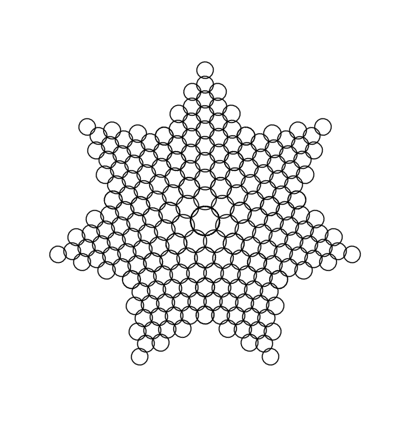
Now we turn our attention to the limiting cases $\alpha=1/2$ and $\alpha=0$ .

7.1 Case $\alpha=\frac{1}{2}$ , $\gamma=0$ : hexagonal $z^{3/2}$ and $\log z$

It is easy to see that the quantities $g(k)$ , $k\geq 1$ , and $v(k)$ , $k\geq 2$ , become singular as $\alpha\to\frac{1}{2}$ (see (6.24) and (6.23)). As a compensation, the quantities $h(k)$ , $k\geq 1$ , vanish with $\alpha\to\frac{1}{2}$ , so that $w(k)\to w(1)=1$ for all $k\geq 2$ . Similar effects hold for the $\ell$ –axis, where $v(\ell\omega)$ , $\ell\geq 2$ , become singular, and $w(\ell\omega)\to 1$ for all $\ell\geq 1$ . (Recall that for the $w$ pattern we have: $w(\omega)=e^{2\pi i\gamma}\to 1$ ). These observations suggest the following rescaling:

u=\overset{\circ}{u},\qquad v=\overset{\circ}{v}/(1-2\alpha),\qquad w=1+(1-2\alpha)\overset{\circ}{w}.

(7.1)

In order to be able to go to the limit $\alpha\to\frac{1}{2}$ , we have to calculate the values of our fields in several lattice points next to ${{z}}=0$ . Applying formulas (4.13), (4.11), we find:

$\displaystyle u(0)=0,\quad u(1)=1,$	$\displaystyle u(\omega)=e^{2\pi i\alpha},\qquad u(1+\omega)=1+e^{2\pi i\alpha},$	(7.2)
$\displaystyle v(0)=0,\quad v(1)=1,$	$\displaystyle v(\omega)=e^{2\pi i\alpha},\qquad v(1+\omega)=\frac{e^{2\pi i\alpha}}{1+e^{2\pi i\alpha}},$	(7.3)
$\displaystyle w(0)=0,\quad w(1)=1,$	$\displaystyle w(\omega)=e^{2\pi i(1-2\alpha)},\quad w(1+\omega)=e^{\pi i(1-2\alpha)}.$	(7.4)

For the rescaled variables $\overset{\circ}{u}$ , $\overset{\circ}{v}$ , $\overset{\circ}{w}$ in the limit $\alpha\to\frac{1}{2}$ we find:

$\displaystyle\overset{\circ}{u}(0)=0,\quad\overset{\circ}{u}(1)=1,$	$\displaystyle\overset{\circ}{u}(\omega)=-1,\quad\overset{\circ}{u}(1+\omega)=0,$	(7.5)
$\displaystyle\overset{\circ}{v}(0)=0,\quad\overset{\circ}{v}(1)=0,$	$\displaystyle\overset{\circ}{v}(\omega)=0,\qquad\overset{\circ}{v}(1+\omega)=\frac{i}{\pi},$	(7.6)
$\displaystyle\overset{\circ}{w}(0)=\infty,\quad\overset{\circ}{w}(1)=0,$	$\displaystyle\overset{\circ}{w}(\omega)=2\pi i,\quad\overset{\circ}{w}(1+\omega)=\pi i.$	(7.7)

These initial values have to be supplemented by the values in all further points of the $k$ – and $\ell$ –axes. From the formulas of Theorem 23 there follows:

\overset{\circ}{u}(3k)=\frac{2^{k}k!}{(2k-1)!!}\cdot(2k),\quad\overset{\circ}{u}(3k+1)=\frac{2^{k}k!}{(2k-1)!!}\cdot(2k+1),\quad\overset{\circ}{u}(3k+2)=\frac{2^{k}k!}{(2k-1)!!}\cdot(2k+2),

(7.8)

\overset{\circ}{f}(3k-1)=\overset{\circ}{f}(3k)=\overset{\circ}{f}(3k+1)=\frac{2^{k}k!}{(2k-1)!!},

(7.9)

and

\overset{\circ}{v}(3k-1)=\frac{(2k-1)!!}{2^{k}(k-1)!}\cdot(2k-1),\quad\overset{\circ}{v}(3k)=\frac{(2k-1)!!}{2^{k}(k-1)!}\cdot(2k),\quad\overset{\circ}{v}(3k+1)=\frac{(2k-1)!!}{2^{k}(k-1)!}\cdot(2k+1),

(7.10)

\overset{\circ}{g}(3k-2)=\overset{\circ}{g}(3k-1)=\overset{\circ}{g}(3k)=\frac{(2k-1)!!}{2^{k}(k-1)!},

(7.11)

which have to be augmented by $\overset{\circ}{u}(k\omega)=-\overset{\circ}{u}(k)$ , $\overset{\circ}{v}(k\omega)=-\overset{\circ}{v}(k)$ . From Corollary 24 there follow the formulas for the edges of the $\overset{\circ}{w}$ lattice:

	$\displaystyle\overset{\circ}{h}(3k-1)=\overset{\circ}{h}(3k)$	$\displaystyle=$	$\displaystyle\overset{\circ}{h}((3k-1)\omega)=\overset{\circ}{h}(3k\omega)\;\;=\;\;\frac{1}{k},\qquad k\geq 1,$		(7.12)
	$\displaystyle\overset{\circ}{h}(3k+1)$	$\displaystyle=$	$\displaystyle\overset{\circ}{h}((3k+1)\omega)\;\;=\;\;\frac{1}{k+1/2},\qquad k\geq 0.$		(7.13)

Definition 27

The hexagonal circle patterns corresponding to the solutions of the $fgh$ –system in the sector (6.7) defined by the boundary values (7.5)–(7.13) are called:

$\overset{\circ}{u}$ , $\overset{\circ}{v}:$

the hexagonal $z^{3/2}$ with an intersection point at the origin;
$\overset{\circ}{w}:$

the symmetric hexagonal $\log z$ .

Alternatively, one could define the lattices $\overset{\circ}{u}$ , $\overset{\circ}{v}$ , $\overset{\circ}{w}$ as the solutions of the $fgh$ –system with the initial values (7.5)–(7.7), satisfying the constraint (5.5), (5.6) with $\alpha=\beta=1/2$ . In this appoach the values (7.8)–(7.13) would be derived from the constraint. Notice also that the formulas (5.7), (5.9) in this case turns into

	$\displaystyle 1$	$\displaystyle=$	$\displaystyle k\frac{1}{\overset{\circ}{f}_{0}\overset{\circ}{g}_{0}+\overset{\circ}{g}_{0}\overset{\circ}{f}_{3}+\overset{\circ}{f}_{3}\overset{\circ}{g}_{3}}+\ell\frac{1}{\overset{\circ}{f}_{2}\overset{\circ}{g}_{2}+\overset{\circ}{g}_{2}\overset{\circ}{f}_{5}+\overset{\circ}{f}_{5}\overset{\circ}{g}_{5}}+m\frac{1}{\overset{\circ}{f}_{4}\overset{\circ}{g}_{4}+\overset{\circ}{g}_{4}\overset{\circ}{f}_{1}+\overset{\circ}{f}_{1}\overset{\circ}{g}_{1}}$		(7.14)
		$\displaystyle=$	$\displaystyle k\frac{\overset{\circ}{h}_{0}\overset{\circ}{f}_{0}\overset{\circ}{h}_{3}}{\overset{\circ}{h}_{0}\overset{\circ}{f}_{0}+\overset{\circ}{f}_{0}\overset{\circ}{h}_{3}+\overset{\circ}{h}_{3}\overset{\circ}{f}_{3}}+\ell\frac{\overset{\circ}{h}_{2}\overset{\circ}{f}_{2}\overset{\circ}{h}_{5}}{\overset{\circ}{h}_{2}\overset{\circ}{f}_{2}+\overset{\circ}{f}_{2}\overset{\circ}{h}_{5}+\overset{\circ}{h}_{5}\overset{\circ}{f}_{5}}+m\frac{\overset{\circ}{h}_{4}\overset{\circ}{f}_{4}\overset{\circ}{h}_{1}}{\overset{\circ}{h}_{4}\overset{\circ}{f}_{4}+\overset{\circ}{f}_{4}\overset{\circ}{h}_{1}+\overset{\circ}{h}_{1}\overset{\circ}{f}_{1}}.$		(7.15)

7.2 Case $\alpha=0$ , $\gamma=1$ : hexagonal $\log z$ and $z^{3}$

Considerations similar to those of the previous subsection show that, as $\alpha\to 0$ , the quantities $h(k)$ , $k\geq 1$ , and $w(k)$ , $k\geq 2$ , become singular (see (6.27) and (6.26)). As a compensation, the quantities $f(k)$ , $k\geq 2$ , and $g(k)$ , $k\geq 1$ , vanish with $\alpha\to 0$ , so that $u(k)\to u(2)=2$ for all $k\geq 3$ , and $v(k)\to v(1)=1$ for all $k\geq 2$ . Similar effects hold for the $\ell$ –axis. These observations suggest the following rescaling:

u=2+2\alpha\overset{\circ}{u},\qquad v=1+\alpha\overset{\circ}{v},\qquad w=\overset{\circ}{w}/(2\alpha^{2}).

(7.16)

It turns out that in this case we need to calculate the values of these functions in a larger number of lattice points in the vicinity of ${{z}}=0$ . To this end, we add to (7.2)–(7.4) the following values, which are obtained by a direct calculation:

	$\displaystyle u(2)=2,\qquad u(2\omega)=2e^{2\pi i\alpha},$		$\displaystyle u(2+\omega)=\frac{1+e^{2\pi i\alpha}}{1+\alpha(e^{2\pi i\alpha}-1)},$		(7.17)
	$\displaystyle u(1+2\omega)=\frac{1+e^{2\pi i\alpha}}{1+\alpha(e^{-2\pi i\alpha}-1)},$		$\displaystyle u(2+2\omega)=\frac{1-\alpha}{1-2\alpha}\,(1+e^{2\pi i\alpha}),$		(7.18)

	$\displaystyle v(2)=\frac{1-\alpha}{1-2\alpha},\qquad v(2\omega)=\frac{1-\alpha}{1-2\alpha}\,e^{2\pi i\alpha},$		$\displaystyle v(2+\omega)=\frac{1}{1+\alpha(e^{-2\pi i\alpha}-1)},$		(7.19)
	$\displaystyle v(1+2\omega)=\frac{e^{2\pi i\alpha}}{1+\alpha(e^{2\pi i\alpha}-1)},$		$\displaystyle v(2+2\omega)=\frac{2e^{2\pi i\alpha}}{1+e^{2\pi i\alpha}}$		(7.20)

	$\displaystyle w(2)=\frac{1-\alpha}{\alpha},\qquad w(2\omega)=\frac{1-\alpha}{\alpha}\,e^{-2\pi i\alpha},$		$\displaystyle w(2+\omega)=-\frac{1}{\alpha(e^{2\pi i\alpha}-1)},$		(7.21)
	$\displaystyle w(1+2\omega)=\frac{e^{-2\pi i\alpha}}{\alpha(e^{2\pi i\alpha}-1)},$		$\displaystyle w(2+2\omega)=-\frac{1-\alpha}{\alpha}\,e^{-2\pi i\alpha}.$		(7.22)

From (7.2)–(7.4) and (7.17)–(7.22) we obtain in the limit $\alpha\to 0$ under the rescaling (7.16) the following initial values:

	$\displaystyle\overset{\circ}{u}(0)=\infty,\quad\overset{\circ}{u}(1)=\infty,\quad\overset{\circ}{u}(\omega)=\infty,\quad\overset{\circ}{u}(2)=0,\quad\overset{\circ}{u}(2\omega)=2\pi i,$		(7.23)
	$\displaystyle\overset{\circ}{u}(1+\omega)=\pi i,\quad\overset{\circ}{u}(2+\omega)=\pi i,\quad\overset{\circ}{u}(1+2\omega)=\pi i,\quad\overset{\circ}{u}(2+2\omega)=1+\pi i,$		(7.24)

	$\displaystyle\overset{\circ}{v}(0)=\infty,\quad\overset{\circ}{v}(1)=0,\quad\overset{\circ}{v}(\omega)=2\pi i,\quad\overset{\circ}{v}(2)=1,\quad\overset{\circ}{v}(2\omega)=1+2\pi i,$		(7.25)
	$\displaystyle\overset{\circ}{v}(1+\omega)=\infty,\quad\overset{\circ}{v}(2+\omega)=0,\quad\overset{\circ}{v}(1+2\omega)=2\pi i,\quad\overset{\circ}{v}(2+2\omega)=\pi i,$		(7.26)

	$\displaystyle\overset{\circ}{w}(0)=0,\quad\overset{\circ}{w}(1)=0,\quad\overset{\circ}{w}(\omega)=0,\quad\overset{\circ}{w}(2)=0,\quad\overset{\circ}{w}(2\omega)=0,$		(7.27)
	$\displaystyle\overset{\circ}{w}(1+\omega)=0,\quad\overset{\circ}{w}(2+\omega)=\frac{i}{\pi},\quad\overset{\circ}{w}(1+2\omega)=-\frac{i}{\pi},\quad\overset{\circ}{w}(2+2\omega)=0.$		(7.28)

These initial values have to be supplemented by the values in all further points of the $k$ – and $\ell$ –axes. From the formulas of Theorem 23 there follow the expressions for the edges of the lattices $\overset{\circ}{u}$ , $\overset{\circ}{v}$ :

	$\displaystyle\overset{\circ}{f}(3k-1)=\overset{\circ}{f}(3k)=\overset{\circ}{f}(3k+1)\;\;=\;\;\overset{\circ}{f}((3k-1)\omega)=\overset{\circ}{f}(3k\omega)=\overset{\circ}{f}((3k+1)\omega)$	$\displaystyle=$	$\displaystyle\frac{1}{k},\qquad k\geq 1,$
	$\displaystyle\overset{\circ}{g}(3k-2)=\overset{\circ}{g}(3k-1)=\overset{\circ}{g}(3k)\;\;=\;\;\overset{\circ}{g}((3k-2)\omega)=\overset{\circ}{g}((3k-1)\omega)=\overset{\circ}{g}(3k\omega)$	$\displaystyle=$	$\displaystyle\frac{1}{k},\qquad k\geq 1.$

The formulas of Corollary 24 yield the results for the lattice $\overset{\circ}{w}$ :

\overset{\circ}{w}(3k)=k^{3},\quad\overset{\circ}{w}(3k+1)=k^{2}(k+1),\quad\overset{\circ}{w}(3k+2)=k(k+1)^{2},\quad k\geq 1,

(7.31)

so that

\overset{\circ}{h}(3k-1)=\overset{\circ}{h}(3k)=k^{2},\quad\overset{\circ}{h}(3k+1)=k(k+1),\quad k\geq 1.

(7.32)

Of course, one has also $\overset{\circ}{w}(k\omega)=\overset{\circ}{w}(k)$ .

Definition 28

The hexagonal circle patterns corresponding to the solutions of the $fgh$ –system in the sector (6.7) defined by the boundary values (7.23)–(7.32) are called:

$\overset{\circ}{u}$ , $\overset{\circ}{v}:$

the asymmetric hexagonal $\log z$ ;
$\overset{\circ}{w}:$

the hexagonal $z^{3}$ with a (degenerate) circle at the origin.

It is meant that the $u$ –image of the half-sector $0\leq{\rm arg}({{z}})\leq\pi/3$ is not symmetric with respect to the line $\Im(u)=\pi i/2$ (the image of ${\rm arg}({{z}})=\pi/6$ , and the same for $v$ . Instead, this symmetry interchanges the $u$ pattern and the $v$ pattern, see Fig. 12.

Alternatively, one can define these lattices as the solutions of the $fgh$ –system with the initial values (7.23)–(7.28), satisfying the constraint (5.5), (5.6), which in the present situation degenerates into

	$\displaystyle 1$	$\displaystyle=$	$\displaystyle k\frac{\overset{\circ}{f}_{0}\overset{\circ}{g}_{0}\overset{\circ}{f}_{3}}{\overset{\circ}{f}_{0}\overset{\circ}{g}_{0}+\overset{\circ}{g}_{0}\overset{\circ}{f}_{3}+\overset{\circ}{f}_{3}\overset{\circ}{g}_{3}}+\ell\frac{\overset{\circ}{f}_{2}\overset{\circ}{g}_{2}\overset{\circ}{f}_{5}}{\overset{\circ}{f}_{2}\overset{\circ}{g}_{2}+\overset{\circ}{g}_{2}\overset{\circ}{f}_{5}+\overset{\circ}{f}_{5}\overset{\circ}{g}_{5}}+m\frac{\overset{\circ}{f}_{4}\overset{\circ}{g}_{4}\overset{\circ}{f}_{1}}{\overset{\circ}{f}_{4}\overset{\circ}{g}_{4}+\overset{\circ}{g}_{4}\overset{\circ}{f}_{1}+\overset{\circ}{f}_{1}\overset{\circ}{g}_{1}},$		(7.33)
	$\displaystyle 1$	$\displaystyle=$	$\displaystyle k\frac{\overset{\circ}{g}_{0}\overset{\circ}{f}_{3}\overset{\circ}{g}_{3}}{\overset{\circ}{f}_{0}\overset{\circ}{g}_{0}+\overset{\circ}{g}_{0}\overset{\circ}{f}_{3}+\overset{\circ}{f}_{3}\overset{\circ}{g}_{3}}+\ell\frac{\overset{\circ}{g}_{2}\overset{\circ}{f}_{5}\overset{\circ}{g}_{5}}{\overset{\circ}{f}_{2}\overset{\circ}{g}_{2}+\overset{\circ}{g}_{2}\overset{\circ}{f}_{5}+\overset{\circ}{f}_{5}\overset{\circ}{g}_{5}}+m\frac{\overset{\circ}{g}_{4}\overset{\circ}{f}_{1}\overset{\circ}{g}_{1}}{\overset{\circ}{f}_{4}\overset{\circ}{g}_{4}+\overset{\circ}{g}_{4}\overset{\circ}{f}_{1}+\overset{\circ}{f}_{1}\overset{\circ}{g}_{1}}.$		(7.34)

Just as in the non–degenerate case, these formulas allow one to calculate inductively the values of $\overset{\circ}{u}$ , $\overset{\circ}{v}$ on the $k$ – and $\ell$ –axes. The formulas (5.7), (5.9) hold literally with $\gamma=1$ .

8 Conclusions

In this paper we introduced the notion of hexagonal circle patterns, and studied in some detail a subclass consisting of circle patterns with the property that six intersection points on each circle have the multi-ratio $-1$ . We established the connection of this subclass with integrable systems on the regular triangular lattice, and used this connection to describe some Bäcklund–like transformations of hexagonal circle patterns (transformation $u\mapsto v\mapsto w$ , see Theorems 13, 14), and to find discrete analogs of the functions $z^{\alpha}$ , $\log z$ . Of course, this is only the beginning of the story of hexagonal circle patterns. In a subsequent publication we shall demonstrate that there exists another subclass related to integrable systems, namely the patterns with fixed intersection angles. The intersection of both subclasses constitute conformally symmetric patterns, including analogs of Doyle’s spirals (cf. [BH]).

A very interesting question is, what part of the theory of integrable circle patterns can be applied to hexagonal circle packings. This also will be a subject of our investigation.

This research was financially supported by DFG (Sonderforschungsbereich 288 “Differential Geometry and Quantum Physics”).

A Appendix: Square lattice version of the $fgh$ –system

Dropping all edges of $E({\cal T}{\cal L})$ parallel to the $m$ –axis, we end up with the cell complex isomorphic to the regular square lattice: its vertices ${{z}}=k+\ell\omega$ may be identified with $(k,\ell)\in{{Z}}^{2}$ , its edges are then identified with those pairs $[(k_{1},\ell_{1}),(k_{2},\ell_{2})]$ for which $|k_{1}-k_{2}|+|\ell_{1}-\ell_{2}|=1$ , and its 2-cells (parallelograms) are identified with the elementary squares of the square lattice. Hence, flat connections on ${\cal T}{\cal L}$ form a subclass of flat connections on the square lattice. A natural question is, whether this inclusion is strict, i.e. whether there exist flat connections on the square lattice which cannot be extended to flat connections on ${\cal T}{\cal L}$ . At least for the $fgh$ –system, the answer is negative: denote by ${\cal M}\subset{\rm SL}(3,{{C}})[\lambda]$ the set of matrices (4.2), then flat connections on the regular square grid with values in ${\cal M}$ are essentially in a one-to-one correspondence with flat connections on ${\cal T}{\cal L}$ with values in ${\cal M}$ , i.e. with solutions of the $fgh$ –system. This is a consequence of the following statement dealing with an elementary square of the regular square lattice: a flat connection on such an elementary square with values in ${\cal M}$ can be extended by an element of ${\cal M}$ sitting on its diagonal without violating the flatness property. More precisely:

Lemma 29

Let

L_{1}L_{2}=L_{3}L_{4},\quad where\quad L_{i}\in{\cal M}\;\;(i=1,2,3,4),

and let the off–diagonal parts of $L_{1}$ , $L_{2}$ be componentwise distinct from the off–diagonal parts of $L_{3}$ , $L_{4}$ , respectively. Then there exists $L_{0}\in{\cal M}$ such that

L_{0}L_{1}L_{2}=L_{0}L_{3}L_{4}=I.

Figure 13: To Lemma 29.

Proof. We have to prove that $(L_{1}L_{2})^{-1}=(L_{3}L_{4})^{-1}\in{\cal M}$ . It is easy to see that it is necessary and sufficient to prove that the entries 13, 21, 32 of this matrix vanish, i.e. that there holds

f_{1}g_{1}+f_{2}g_{1}+f_{2}g_{2}=f_{3}g_{3}+f_{4}g_{3}+f_{4}g_{4}=0,

(A.1)

as well as two similar equations resulting by two successive permutations $(f,g,h)\mapsto(g,h,f)$ . We are given the relations $f_{i}g_{i}h_{i}=1$ and

f_{1}+f_{2}=f_{3}+f_{4},\qquad g_{1}+g_{2}=g_{3}+g_{4},\qquad h_{1}+h_{2}=h_{3}+h_{4},

(A.2)

f_{1}g_{2}=f_{3}g_{4},\qquad g_{1}h_{2}=g_{3}h_{4},\qquad h_{1}f_{2}=h_{3}f_{4}.

(A.3)

In order to prove (A.1), we start with the third equation in (A.2):

h_{1}\left(1-\frac{h_{3}}{h_{1}}\right)=h_{2}\left(\frac{h_{4}}{h_{2}}-1\right).

(A.4)

Using $f_{i}g_{i}h_{i}=1$ and (A.3), we find:

\frac{h_{3}}{h_{1}}=\frac{f_{1}g_{1}}{f_{3}g_{3}}=\frac{g_{4}g_{1}}{g_{2}g_{3}},\qquad\frac{h_{4}}{h_{2}}=\frac{g_{1}}{g_{3}}.

(A.5)

Plugging this into (A.4), we get:

\frac{g_{2}g_{3}-g_{1}g_{4}}{f_{1}g_{1}g_{2}g_{3}}=\frac{g_{1}-g_{3}}{f_{2}g_{2}g_{3}}.

(A.6)

Now, due to the second equation in (A.2), we find:

g_{2}g_{3}-g_{1}g_{4}=g_{2}(g_{3}-g_{1})+g_{1}(g_{2}-g_{4})=(g_{1}+g_{2})(g_{3}-g_{1}).

(A.7)

Substituting this into (A.6), we come to the equation:

(g_{3}-g_{1})\left(\frac{g_{1}+g_{2}}{f_{1}g_{1}}+\frac{1}{f_{2}}\right)=0.

(A.8)

Since, by condition, $g_{1}\neq g_{3}$ , we obtain $f_{2}(g_{1}+g_{2})+f_{1}g_{1}=0$ , which is the equation (A.1).

This result shows that the $fgh$ –system could be alternatively studied in a more common framework of integrable systems on a square lattice. However, such an approach would hide a rich and interesting geometric structures immanently connected with the triangular lattice. It should be said at this point that the one–field equation (4.22) was first found, under the name of the “Schwarzian lattice Bussinesq equation” by Nijhoff in [N] using a (different) Lax representation on the square lattice. The same holds for the one–field form of the constraint (5.10).

B Appendix: Proofs of statements of Sect. 5

Proof of Proposition 15. The arguments are similar for both equations (5.5), (5.6). For instance, for the first one we have to demonstrate that

	$\displaystyle\frac{f_{0}g_{0}f_{3}}{f_{0}g_{0}+g_{0}f_{3}+f_{3}g_{3}}+\frac{f_{2}g_{2}f_{5}}{f_{2}g_{2}+g_{2}f_{5}+f_{5}g_{5}}+\frac{f_{4}g_{4}f_{1}}{f_{4}g_{4}+g_{4}f_{1}+f_{1}g_{1}}$	$\displaystyle=$
	$\displaystyle\frac{f_{0}f_{3}}{f_{0}+f_{3}+f_{3}g_{3}/g_{0}}+\frac{f_{2}f_{5}}{f_{2}+f_{5}+f_{5}g_{5}/g_{2}}+\frac{f_{4}f_{1}}{f_{4}+f_{1}+f_{1}g_{1}/g_{4}}$	$\displaystyle=$	$\displaystyle 0.$		(B.1)

To eliminate the fields $g$ from this equation, consider six elementary triangles surrounding the vertex ${{z}}$ . The equations (4.4) imply:

	$\displaystyle\frac{g_{1}}{g_{0}}=-\frac{f_{0}+f_{1}}{f_{1}},\quad\frac{g_{2}}{g_{1}}=-\frac{f_{1}}{f_{1}+f_{2}},\quad\frac{g_{3}}{g_{2}}=-\frac{f_{2}+f_{3}}{f_{3}},$
	$\displaystyle\frac{g_{5}}{g_{0}}=-\frac{f_{5}+f_{0}}{f_{5}},\quad\frac{g_{4}}{g_{5}}=-\frac{f_{5}}{f_{4}+f_{5}},\quad\frac{g_{3}}{g_{2}}=-\frac{f_{3}+f_{4}}{f_{3}}.$

Therefore,

	$\displaystyle f_{0}+f_{3}+f_{3}\frac{g_{3}}{g_{0}}$	$\displaystyle=$	$\displaystyle f_{0}+f_{3}-\frac{(f_{0}+f_{1})(f_{2}+f_{3})}{f_{1}+f_{2}}=\frac{(f_{0}-f_{2})(f_{1}-f_{3})}{f_{1}+f_{2}}$		(B.2)
		$\displaystyle=$	$\displaystyle f_{0}+f_{3}-\frac{(f_{5}+f_{0})(f_{3}+f_{4})}{f_{4}+f_{5}}=\frac{(f_{4}-f_{0})(f_{3}-f_{5})}{f_{4}+f_{5}}.$		(B.3)

By the way, this again yields the property $MR=-1$ of the lattice $u$ , which can be written now as

(f_{0}+f_{1})(f_{2}+f_{3})(f_{4}+f_{5})=(f_{1}+f_{2})(f_{3}+f_{4})(f_{5}+f_{0}),

(B.4)

Using (B.2), an analogous expression along the $\ell$ –axis, and an expression analogous to (B.3) along the $m$ –axis, we rewrite (B) as

\frac{f_{0}f_{3}(f_{1}+f_{2})}{(f_{0}-f_{2})(f_{1}-f_{3})}+\frac{f_{2}f_{5}(f_{3}+f_{4})}{(f_{2}-f_{4})(f_{3}-f_{5})}+\frac{f_{4}f_{1}(f_{2}+f_{3})}{(f_{2}-f_{4})(f_{1}-f_{3})}=0.

(B.5)

Clearing denominators, we put it in the equivalent form

	$\displaystyle f_{0}f_{3}(f_{1}+f_{2})(f_{2}-f_{4})(f_{3}-f_{5})+f_{2}f_{5}(f_{3}+f_{4})(f_{0}-f_{2})(f_{1}-f_{3})$
	$\displaystyle+f_{4}f_{1}(f_{2}+f_{3})(f_{0}-f_{2})(f_{3}-f_{5})$	$\displaystyle=$	$\displaystyle 0.$

But the polynomial on the left–hand side of the last formula is equal to

f_{2}f_{3}\Big((f_{1}+f_{2})(f_{3}+f_{4})(f_{5}+f_{0})-(f_{0}+f_{1})(f_{2}+f_{3})(f_{4}+f_{5})\Big),

and hence vanishes in virtue of (B.4).

Proof of Proposition 16. Denote the right–hand sides of (5.5), (5.6), (5.7) through $U({{z}})$ , $V({{z}})$ , $W({{z}})$ , respectively. In order to prove (5.7), i.e. $\gamma w=W({{z}})$ , it is necessary and sufficient to demonstrate that

\gamma h_{0}=W(\mathaccent 869{{{z}}})-W({{z}}),\quad\gamma h_{2}=W(\mathaccent 866{{{z}}})-W({{z}}),\quad\gamma h_{4}=W(\bar{{{z}}})-W({{z}}),

(or, actually, any two of these three equations). We perform the proof for the first one only, since for the other two everything is similar. In dealing with our constraints we are free to choose any representative $(k,\ell,m)$ for ${{z}}$ . In order to keep things shorter, we always assume in this proof that $m=0$ . Writing the formula

\gamma=\frac{1}{h_{0}}\Big(W(\mathaccent 869{{{z}}})-W({{z}})\Big)

in long hand, we have to prove that

	$\displaystyle\gamma=1-\alpha-\beta$	$\displaystyle=$	$\displaystyle(k+1)\frac{1/h_{0}}{\mathaccent 869{f}_{0}\mathaccent 869{g}_{0}+\mathaccent 869{g}_{0}\mathaccent 869{f}_{3}+\mathaccent 869{f}_{3}\mathaccent 869{g}_{3}}-k\frac{1/h_{0}}{f_{0}g_{0}+g_{0}f_{3}+f_{3}g_{3}}$		(B.6)
			$\displaystyle+\ell\frac{1/h_{0}}{\mathaccent 869{f}_{2}\mathaccent 869{g}_{2}+\mathaccent 869{g}_{2}\mathaccent 869{f}_{5}+\mathaccent 869{f}_{5}\mathaccent 869{g}_{5}}-\ell\frac{1/h_{0}}{f_{2}g_{2}+g_{2}f_{5}+f_{5}g_{5}}.$		(B.6)

Assuming that (5.5) and (5.6) hold, we have:

\alpha+\beta=\frac{1}{f_{0}}\Big(U(\mathaccent 869{{{z}}})-U({{z}})\Big)+\frac{1}{g_{0}}\Big(V(\mathaccent 869{{{z}}})-V({{z}})\Big).

Taking into account that $\mathaccent 869{f}_{3}=f_{0}$ , $\mathaccent 869{g}_{3}=g_{0}$ , we find:

	$\displaystyle\alpha+\beta$	$\displaystyle=$	$\displaystyle(k+1)\frac{\mathaccent 869{f}_{0}\mathaccent 869{g}_{0}+\mathaccent 869{g}_{0}\mathaccent 869{f}_{3}}{\mathaccent 869{f}_{0}\mathaccent 869{g}_{0}+\mathaccent 869{g}_{0}\mathaccent 869{f}_{3}+\mathaccent 869{f}_{3}\mathaccent 869{g}_{3}}-k\frac{g_{0}f_{3}+f_{3}g_{3}}{f_{0}g_{0}+g_{0}f_{3}+f_{3}g_{3}}$
			$\displaystyle+\ell\left(\frac{\mathaccent 869{f}_{2}\mathaccent 869{g}_{2}\mathaccent 869{f}_{5}/f_{0}+\mathaccent 869{g}_{2}\mathaccent 869{f}_{5}\mathaccent 869{g}_{5}/g_{0}}{\mathaccent 869{f}_{2}\mathaccent 869{g}_{2}+\mathaccent 869{g}_{2}\mathaccent 869{f}_{5}+\mathaccent 869{f}_{5}\mathaccent 869{g}_{5}}-\frac{f_{2}g_{2}f_{5}/f_{0}+g_{2}f_{5}g_{5}/g_{0}}{f_{2}g_{2}+g_{2}f_{5}+f_{5}g_{5}}\right),$

or, equivalently,

	$\displaystyle\gamma=1-\alpha-\beta$	$\displaystyle=$	$\displaystyle(k+1)\frac{\mathaccent 869{f}_{3}\mathaccent 869{g}_{3}}{\mathaccent 869{f}_{0}\mathaccent 869{g}_{0}+\mathaccent 869{g}_{0}\mathaccent 869{f}_{3}+\mathaccent 869{f}_{3}\mathaccent 869{g}_{3}}-k\frac{f_{0}g_{0}}{f_{0}g_{0}+g_{0}f_{3}+f_{3}g_{3}}$		(B.7)
			$\displaystyle-\ell\left(\frac{\mathaccent 869{f}_{2}\mathaccent 869{g}_{2}\mathaccent 869{f}_{5}/f_{0}+\mathaccent 869{g}_{2}\mathaccent 869{f}_{5}\mathaccent 869{g}_{5}/g_{0}}{\mathaccent 869{f}_{2}\mathaccent 869{g}_{2}+\mathaccent 869{g}_{2}\mathaccent 869{f}_{5}+\mathaccent 869{f}_{5}\mathaccent 869{g}_{5}}-\frac{f_{2}g_{2}f_{5}/f_{0}+g_{2}f_{5}g_{5}/g_{0}}{f_{2}g_{2}+g_{2}f_{5}+f_{5}g_{5}}\right).$		(B.7)

The first two terms on the right–hand side already have the required form, since $\mathaccent 869{f}_{3}\mathaccent 869{g}_{3}=f_{0}g_{0}=1/h_{0}$ . So, it remains to prove that

-\frac{\mathaccent 869{f}_{2}\mathaccent 869{g}_{2}\mathaccent 869{f}_{5}/f_{0}+\mathaccent 869{g}_{2}\mathaccent 869{f}_{5}\mathaccent 869{g}_{5}/g_{0}}{\mathaccent 869{f}_{2}\mathaccent 869{g}_{2}+\mathaccent 869{g}_{2}\mathaccent 869{f}_{5}+\mathaccent 869{f}_{5}\mathaccent 869{g}_{5}}+\frac{f_{2}g_{2}f_{5}/f_{0}+g_{2}f_{5}g_{5}/g_{0}}{f_{2}g_{2}+g_{2}f_{5}+f_{5}g_{5}}=\frac{1/h_{0}}{\mathaccent 869{f}_{2}\mathaccent 869{g}_{2}+\mathaccent 869{g}_{2}\mathaccent 869{f}_{5}+\mathaccent 869{f}_{5}\mathaccent 869{g}_{5}}-\frac{1/h_{0}}{f_{2}g_{2}+g_{2}f_{5}+f_{5}g_{5}}.

(B.8)

The most direct and unambiguous way to do this is to notice that everything here may be expressed with the help of the $fgh$ –equations in terms of a single field $h$ . After straightforward calculations one obtains:

$\displaystyle\mathaccent 869{f}_{2}\mathaccent 869{g}_{2}\frac{\mathaccent 869{f}_{5}}{f_{0}}+\mathaccent 869{f}_{5}\mathaccent 869{g}_{5}\frac{\mathaccent 869{g}_{2}}{g_{0}}$	$\displaystyle=$	$\displaystyle-\frac{1}{\mathaccent 869{h}_{5}}+\frac{h_{0}(h_{0}-\mathaccent 869{h}_{5})}{\mathaccent 869{h}_{2}\mathaccent 869{h}_{5}h_{5}},$	(B.9)
$\displaystyle f_{2}g_{2}\frac{f_{5}}{f_{0}}+f_{5}g_{5}\frac{g_{2}}{g_{0}}$	$\displaystyle=$	$\displaystyle-\frac{1}{h_{2}}+\frac{h_{0}(h_{0}-h_{2})}{\mathaccent 869{h}_{2}h_{2}h_{5}},$	(B.10)
$\displaystyle\mathaccent 869{f}_{2}\mathaccent 869{g}_{2}+\mathaccent 869{g}_{2}\mathaccent 869{f}_{5}+\mathaccent 869{f}_{5}\mathaccent 869{g}_{5}$	$\displaystyle=$	$\displaystyle\frac{(h_{0}-\mathaccent 869{h}_{5})(\mathaccent 869{h}_{4}-\mathaccent 869{h}_{2})}{\mathaccent 869{h}_{2}\mathaccent 869{h}_{5}h_{5}},$	(B.11)
$\displaystyle f_{2}g_{2}+g_{2}f_{5}+f_{5}g_{5}$	$\displaystyle=$	$\displaystyle\frac{(h_{0}-h_{2})(h_{1}-h_{5})}{\mathaccent 869{h}_{2}h_{2}h_{5}}.$	(B.12)

Taking into account that $\mathaccent 869{h}_{4}-\mathaccent 869{h}_{2}=h_{1}-h_{5}$ , we see that (B.8) and Proposition 16 are proved.

Proof of Theorem 19. In order for the isomonodromy property to hold, the following compatibility conditions of (5.16) with (5.17) are necessary and sufficient: (5.14) and

\left\{\begin{array}[]{l}\displaystyle\frac{d}{d\mu}{\cal L}({{e}}_{0},\mu)={\cal A}_{k+1,\ell,m}{\cal L}({{e}}_{0},\mu)-{\cal L}({{e}}_{0},\mu){\cal A}_{k,\ell,m},\\ \displaystyle\frac{d}{d\mu}{\cal L}({{e}}_{2},\mu)={\cal A}_{k,\ell+1,m}{\cal L}({{e}}_{2},\mu)-{\cal L}({{e}}_{2},\mu){\cal A}_{k,\ell,m},\\ \displaystyle\frac{d}{d\mu}{\cal L}({{e}}_{4},\mu)={\cal A}_{k,\ell,m+1}{\cal L}({{e}}_{4},\mu)-{\cal L}({{e}}_{4},\mu){\cal A}_{k,\ell,m}.\end{array}\right.

(B.13)

Substituting the ansatz (5.19) and calculating the residues at $\mu=-1$ , $\mu=0$ and $\mu=\infty$ , we see that the above system is equivalent to the following nine matrix equations:

$\displaystyle C_{k+1,\ell,m}{\cal L}({{e}}_{0},-1)$	$\displaystyle=$	$\displaystyle{\cal L}({{e}}_{0},-1)C_{k,\ell,m},$	(B.14)
$\displaystyle C_{k,\ell+1,m}{\cal L}({{e}}_{2},-1)$	$\displaystyle=$	$\displaystyle{\cal L}({{e}}_{2},-1)C_{k,\ell,m},$	(B.15)
$\displaystyle C_{k,\ell,m+1}{\cal L}({{e}}_{4},-1)$	$\displaystyle=$	$\displaystyle{\cal L}({{e}}_{4},-1)C_{k,\ell,m},$	(B.16)

$\displaystyle D(\mathaccent 869{{{z}}}){\cal L}({{e}}_{0},0)$	$\displaystyle=$	$\displaystyle{\cal L}({{e}}_{0},0)D({{z}}),$	(B.17)
$\displaystyle D(\mathaccent 866{{{z}}}){\cal L}({{e}}_{2},0)$	$\displaystyle=$	$\displaystyle{\cal L}({{e}}_{2},0)D({{z}}),$	(B.18)
$\displaystyle D(\bar{{{z}}}){\cal L}({{e}}_{4},0)$	$\displaystyle=$	$\displaystyle{\cal L}({{e}}_{4},0)D({{z}}),$	(B.19)

$\displaystyle\Big(C_{k+1,\ell,m}+D(\mathaccent 869{{{z}}})\Big)Q-Q\Big(C_{k,\ell,m}+D({{z}})\Big)$	$\displaystyle=$	$\displaystyle Q,$	(B.20)
$\displaystyle\Big(C_{k,\ell+1,m}+D(\mathaccent 866{{{z}}})\Big)Q-Q\Big(C_{k,\ell,m}+D({{z}})\Big)$	$\displaystyle=$	$\displaystyle Q,$	(B.21)
$\displaystyle\Big(C_{k,\ell,m+1}+D(\bar{{{z}}})\Big)Q-Q\Big(C_{k,\ell,m}+D({{z}})\Big)$	$\displaystyle=$	$\displaystyle Q,$	(B.22)

where

Q=\left(\begin{array}[]{ccc}0&0&0\\ 0&0&0\\ 1&0&0\end{array}\right).

(B.23)

We do not aim at solving these equations completely, but rather at finding a certain solution leading to the constraint (5.5), (5.6). The subsequent reasoning will be divided into several steps.

Step 1. Consistency of the ansatz for $C_{k,\ell,m}$ . First of all, we have to convince ourselves that the ansatz (5.20), (5.21) does not violate the necessary condition (5.18), i.e. that

P_{2}+P_{4}+P_{6}=I.

(B.24)

Notice that the entries 12 and 23 of this matrix equation are nothing but the content of Proposition 15. Upon the cyclic permutation of the fields $(f,g,h)\mapsto(g,h,f)$ this gives also the entry 31. To check the entry 21, we proceed as in the proof of Proposition 15. We have to prove that

$\displaystyle\frac{g_{0}}{f_{0}g_{0}+g_{0}f_{3}+f_{3}g_{3}}+\frac{g_{2}}{f_{2}g_{2}+g_{2}f_{5}+f_{5}g_{5}}+\frac{g_{4}}{f_{4}g_{4}+g_{4}f_{1}+f_{1}g_{1}}$	$\displaystyle=$
$\displaystyle\frac{1}{f_{0}+f_{3}+f_{3}g_{3}/g_{0}}+\frac{1}{f_{2}+f_{5}+f_{5}g_{5}/g_{2}}+\frac{1}{f_{4}+f_{1}+f_{1}g_{1}/g_{4}}$	$\displaystyle=$
$\displaystyle\frac{f_{1}+f_{2}}{(f_{0}-f_{2})(f_{1}-f_{3})}+\frac{f_{3}+f_{4}}{(f_{2}-f_{4})(f_{3}-f_{5})}+\frac{f_{2}+f_{3}}{(f_{2}-f_{4})(f_{1}-f_{3})}$	$\displaystyle=$	$\displaystyle 0.$

Clearing denominators, we put it in the equivalent form

(f_{1}+f_{2})(f_{2}-f_{4})(f_{3}-f_{5})+(f_{3}+f_{4})(f_{0}-f_{2})(f_{1}-f_{3})+(f_{2}+f_{3})(f_{0}-f_{2})(f_{3}-f_{5})=0.

But the polynomial on the left–hand side is equal to

(f_{1}+f_{2})(f_{3}+f_{4})(f_{5}+f_{0})-(f_{0}+f_{1})(f_{2}+f_{3})(f_{4}+f_{5}),

and vanishes due to (B.4). Via the cyclic permutation of fields this proves also the entries 32 and 13 of the matrix identity (B.24). Finally, turning to the diagonal entries, we consider, for the sake of definiteness, the entry 22. We have to prove that

$\displaystyle\frac{f_{3}g_{0}}{f_{0}g_{0}+g_{0}f_{3}+f_{3}g_{3}}+\frac{f_{5}g_{2}}{f_{2}g_{2}+g_{2}f_{5}+f_{5}g_{5}}+\frac{f_{1}g_{4}}{f_{4}g_{4}+g_{4}f_{1}+f_{1}g_{1}}$	$\displaystyle=$
$\displaystyle\frac{f_{3}}{f_{0}+f_{3}+f_{3}g_{3}/g_{0}}+\frac{f_{5}}{f_{2}+f_{5}+f_{5}g_{5}/g_{2}}+\frac{f_{1}}{f_{4}+f_{1}+f_{1}g_{1}/g_{4}}$	$\displaystyle=$
$\displaystyle\frac{f_{3}(f_{1}+f_{2})}{(f_{0}-f_{2})(f_{1}-f_{3})}+\frac{f_{5}(f_{3}+f_{4})}{(f_{2}-f_{4})(f_{3}-f_{5})}+\frac{f_{1}(f_{2}+f_{3})}{(f_{2}-f_{4})(f_{1}-f_{3})}$	$\displaystyle=$	$\displaystyle 1,$

	$\displaystyle f_{3}(f_{1}+f_{2})(f_{2}-f_{4})(f_{3}-f_{5})+f_{5}(f_{3}+f_{4})(f_{0}-f_{2})(f_{1}-f_{3})$	$\displaystyle+$
	$\displaystyle f_{1}(f_{2}+f_{3})(f_{0}-f_{2})(f_{3}-f_{5})-(f_{0}-f_{2})(f_{1}-f_{3})(f_{2}-f_{4})(f_{3}-f_{5})$	$\displaystyle=$	$\displaystyle 0.$

Again, the polynomial on the left–hand side is equal to

f_{3}\Big((f_{1}+f_{2})(f_{3}+f_{4})(f_{5}+f_{0})-(f_{0}+f_{1})(f_{2}+f_{3})(f_{4}+f_{5})\Big),

and vanishes due to (B.4). The formula (B.24) is proved.

Step 2. Checking the equations for the matrix $C_{k,\ell,m}$ . Next, we have to show that the ansatz (5.20), (5.21) verifies (B.14)–(B.16). Notice that the matrices

{\cal L}({{e}},-1)=\left(\begin{array}[]{ccc}1&f&0\\ 0&1&g\\ -h&0&1\end{array}\right)

are degenerate, and that

\xi=\left(\begin{array}[]{c}fg\\ -g\\ 1\end{array}\right)\quad{\rm and}\quad\eta^{\rm T}=\Big(1,\;\;-f,\;\;fg\Big)

are the right null–vector and the left null–vector of ${\cal L}({{e}},-1)$ , respectively. In terms of these vectors one can write the projectors $P_{0,2,4}$ as

P_{j}=\frac{1}{\langle\xi_{j},\eta_{j+3}\rangle}\xi_{j}\eta_{j+3}^{\rm T},\quad j=0,2,4.

Therefore we have:

$\displaystyle P_{0}(\mathaccent 869{{{z}}}){\cal L}({{e}}_{0},-1)={\cal L}({{e}}_{0},-1)P_{0}({{z}})$	$\displaystyle=$	$\displaystyle 0,$	(B.25)
$\displaystyle P_{2}(\mathaccent 866{{{z}}}){\cal L}({{e}}_{2},-1)={\cal L}({{e}}_{2},-1)P_{2}({{z}})$	$\displaystyle=$	$\displaystyle 0,$	(B.26)
$\displaystyle P_{4}(\bar{{{z}}}){\cal L}({{e}}_{4},-1)={\cal L}({{e}}_{4},-1)P_{4}({{z}})$	$\displaystyle=$	$\displaystyle 0.$	(B.27)

In order to demonstrate (B.14)–(B.16) it is sufficient to prove that

$\displaystyle P_{2}(\mathaccent 869{{{z}}}){\cal L}({{e}}_{0},-1)={\cal L}({{e}}_{0},-1)P_{2}({{z}}),$	$\displaystyle P_{4}(\mathaccent 869{{{z}}}){\cal L}({{e}}_{0},-1)={\cal L}({{e}}_{0},-1)P_{4}({{z}})=0,$	(B.28)
$\displaystyle P_{4}(\mathaccent 866{{{z}}}){\cal L}({{e}}_{2},-1)={\cal L}({{e}}_{2},-1)P_{4}({{z}}),$	$\displaystyle P_{0}(\mathaccent 866{{{z}}}){\cal L}({{e}}_{2},-1)={\cal L}({{e}}_{2},-1)P_{0}({{z}})=0,$	(B.29)
$\displaystyle P_{0}(\bar{{{z}}}){\cal L}({{e}}_{4},-1)={\cal L}({{e}}_{4},-1)P_{0}({{z}}),$	$\displaystyle P_{2}(\bar{{{z}}}){\cal L}({{e}}_{4},-1)={\cal L}({{e}}_{4},-1)P_{2}({{z}})=0.$	(B.30)

All these equations are verified in a similar manner, therefore we restrict ourselves to the first one.

\frac{1}{\langle\mathaccent 869{\xi}_{2},\mathaccent 869{\eta}_{5}\rangle}\mathaccent 869{\xi}_{2}\mathaccent 869{\eta}_{5}^{\rm T}{\cal L}({{e}}_{0},-1)=\frac{1}{\langle\xi_{2},\eta_{5}\rangle}{\cal L}({{e}}_{0},-1)\xi_{2}\eta_{5}^{\rm T},

or, in long hand,

\frac{1}{\mathaccent 869{f}_{2}\mathaccent 869{g}_{2}+\mathaccent 869{g}_{2}\mathaccent 869{f}_{5}+\mathaccent 869{f}_{5}\mathaccent 869{g}_{5}}\left(\begin{array}[]{c}\mathaccent 869{f}_{2}\mathaccent 869{g}_{2}\\ -\mathaccent 869{g}_{2}\\ 1\end{array}\right)\!\left(\begin{array}[]{c}1-h_{0}/\mathaccent 869{h}_{5}\\ f_{0}-\mathaccent 869{f}_{5}\\ \mathaccent 869{f}_{5}(\mathaccent 869{g}_{5}-g_{0})\end{array}\right)^{\rm T}\!\!=\frac{1}{f_{2}g_{2}+g_{2}f_{5}+f_{5}g_{5}}\left(\begin{array}[]{c}(f_{2}-f_{0})g_{2}\\ g_{0}-g_{2}\\ 1-h_{0}/h_{2}\end{array}\right)\!\left(\begin{array}[]{c}1\\ -f_{5}\\ f_{5}g_{5}\end{array}\right)^{\rm T}\!\!.

(B.31)

To prove this we have, first, to check that these two rank one matrices are proportional, and then to check that their entries 31 (say) coincide. The second of these claims reads:

\frac{1-h_{0}/\mathaccent 869{h}_{5}}{\mathaccent 869{f}_{2}\mathaccent 869{g}_{2}+\mathaccent 869{g}_{2}\mathaccent 869{f}_{5}+\mathaccent 869{f}_{5}\mathaccent 869{g}_{5}}=\frac{1-h_{0}/h_{2}}{f_{2}g_{2}+g_{2}f_{5}+f_{5}g_{5}},

(B.32)

and follows from (B.11), (B.12). The first claim above is equivalent to:

\left(\begin{array}[]{c}\mathaccent 869{f}_{2}\mathaccent 869{g}_{2}\\ -\mathaccent 869{g}_{2}\\ 1\end{array}\right)\sim\left(\begin{array}[]{c}(f_{2}-f_{0})g_{2}\\ g_{0}-g_{2}\\ 1-h_{0}/h_{2}\end{array}\right)\quad{\rm and}\quad\left(\begin{array}[]{c}1-h_{0}/\mathaccent 869{h}_{5}\\ f_{0}-\mathaccent 869{f}_{5}\\ \mathaccent 869{f}_{5}(\mathaccent 869{g}_{5}-g_{0})\end{array}\right)\sim\left(\begin{array}[]{c}1\\ -f_{5}\\ f_{5}g_{5}\end{array}\right),

which, in turn, is equivalent to:

\mathaccent 869{f}_{2}=g_{2}\frac{f_{0}-f_{2}}{g_{0}-g_{2}},\quad\mathaccent 869{g}_{2}=h_{2}\frac{g_{0}-g_{2}}{h_{0}-h_{2}},

(B.33)

and

\mathaccent 869{h}_{5}=f_{5}\frac{h_{0}-\mathaccent 869{h}_{5}}{f_{0}-\mathaccent 869{f}_{5}},\quad\mathaccent 869{f}_{5}=g_{5}\frac{f_{0}-\mathaccent 869{f}_{5}}{g_{0}-\mathaccent 869{g}_{5}}.

(B.34)

All these relations easily follow from the equations of the $fgh$ –system. For instance, to check the first equation in (B.33), one has to consider the two elementary positively oriented triangles $({{z}},{{z}}+\omega,{{z}}+\varepsilon)$ and $({{z}},{{z}}+1,{{z}}+\varepsilon)$ . Denoting the edge ${{e}}_{12}=({{z}}+\omega,{{z}}+\varepsilon)$ , we have:

f_{2}+f_{12}=f_{0}+\mathaccent 869{f}_{2}\;(=-f_{1}),\qquad f_{12}g_{2}=\mathaccent 869{f}_{2}g_{0}\;(=f_{1}g_{1}).

Eliminating $f_{12}$ from these two equations, we end up with the desired one. This finishes the proof of (B.14)–(B.16).

Step 3. Checking the equations for the matrix $D({{z}})$ . Notice that the matrices

L({{e}},0)=\left(\begin{array}[]{ccc}1&f&0\\ 0&1&g\\ 0&0&1\end{array}\right)

are upper triangular. We require that the matrices $D({{z}})$ are also upper triangular:

D=\left(\begin{array}[]{ccc}d_{11}&d_{12}&d_{13}\\ 0&d_{22}&d_{23}\\ 0&0&d_{33}\end{array}\right).

It is immediately seen that the diagonal entries are constants. By multiplying the wave function $\Psi_{k,\ell,m}(\mu)$ from the right by a constant ( $\mu$ –dependent) matrix one can arrange that the matrices $D({{z}})$ are traceless. Hence the diagonal part of $D$ is parameterized by two arbitrary numbers. It will be convenient to choose this parametrization as

(d_{11},d_{22},d_{33})=\Big(-(2\alpha+\beta)/3,\;(\alpha-\beta)/3,\;(2\beta+\alpha)/3\Big).

Equating the entries 12 and 23 in (B.17)–(B.19), we find for an arbitrary positively oriented edge ${{e}}=({{z}}_{1},{{z}}_{2})\in E({\cal T}{\cal L})$ :

	$\displaystyle d_{12}({{z}}_{2})-d_{12}({{z}}_{1})$	$\displaystyle=$	$\displaystyle(d_{22}-d_{11})f=\alpha\Big(u({{z}}_{2})-u({{z}}_{1})\Big),$
	$\displaystyle d_{23}({{z}}_{2})-d_{23}({{z}}_{1})$	$\displaystyle=$	$\displaystyle(d_{33}-d_{22})g=\beta\Big(v({{z}}_{2})-v({{z}}_{1})\Big).$

Obviously, a solution (unique up to an additive constant) is given by

d_{12}=\alpha u,\quad d_{23}=\beta v.

Finally, equating in (B.17)–(B.19) the entries 13, we find:

	$\displaystyle d_{13}({{z}}_{2})-d_{13}({{z}}_{1})$	$\displaystyle=$	$\displaystyle d_{23}({{z}}_{1})f-d_{12}({{z}}_{2})g$		(B.35)
		$\displaystyle=$	$\displaystyle\beta v({{z}}_{1})\Big(u({{z}}_{2})-u({{z}}_{1})\Big)-\alpha u({{z}}_{2})\Big(v({{z}}_{2})-v({{z}}_{1})\Big).$		(B.36)

Comparing this with (4.18), (4.21), we see that (5.22) is proved.

Step 4. Equations relating the matrices $C_{k,\ell,m}$ and $D({{z}})$ . It remains to consider the equations (B.20)–(B.22). Denoting entries of the matrix $C$ by $c_{ij}$ , we see that these matrix equations are equivalent to the following scalar ones:

$\displaystyle c_{12}+d_{12}$	$\displaystyle=$	$\displaystyle 0,$	(B.37)
$\displaystyle c_{23}+d_{23}$	$\displaystyle=$	$\displaystyle 0,$	(B.38)
$\displaystyle c_{13}+d_{13}$	$\displaystyle=$	$\displaystyle 0,$	(B.39)

$\displaystyle(c_{33})_{k+1,\ell,m}-(c_{11})_{k,\ell,m}+d_{33}-d_{11}$	$\displaystyle=$	$\displaystyle 1,$	(B.40)
$\displaystyle(c_{33})_{k,\ell+1,m}-(c_{11})_{k,\ell,m}+d_{33}-d_{11}$	$\displaystyle=$	$\displaystyle 1,$	(B.41)
$\displaystyle(c_{33})_{k,\ell,m+1}-(c_{11})_{k,\ell,m}+d_{33}-d_{11}$	$\displaystyle=$	$\displaystyle 1.$	(B.42)

(In the last three equations we took into account that $d_{11}$ , $d_{33}$ are constants.) It is easy to see that the equations (B.37), (B.38) are nothing but the constraint equations (5.5), (5.6), respectively. We show now that the remaining equations (B.39)–(B.42) are not independent, but rather follow from the equations of the $fgh$ –system and the constraints (B.37), (B.38). We start with the last three equations, and prove the claim for (B.40), since for other two everything is similar. As in the proof of Proposition 16, we write the formulas here with $m=0$ . Writing (B.40) in long hand, using the ansätze (5.20), (5.21), (5.22), we see that it is equivalent to

	$\displaystyle 1-\alpha-\beta$	$\displaystyle=$	$\displaystyle(k+1)\frac{1/h_{0}}{\mathaccent 869{f}_{0}\mathaccent 869{g}_{0}+\mathaccent 869{g}_{0}\mathaccent 869{f}_{3}+\mathaccent 869{f}_{3}\mathaccent 869{g}_{3}}-k\frac{1/h_{0}}{f_{0}g_{0}+g_{0}f_{3}+f_{3}g_{3}}$		(B.43)
			$\displaystyle+\ell\frac{1/\mathaccent 869{h}_{5}}{\mathaccent 869{f}_{2}\mathaccent 869{g}_{2}+\mathaccent 869{g}_{2}\mathaccent 869{f}_{5}+\mathaccent 869{f}_{5}\mathaccent 869{g}_{5}}-\ell\frac{1/h_{2}}{f_{2}g_{2}+g_{2}f_{5}+f_{5}g_{5}}.$		(B.43)

But this follows immediately from (B.6), (B.32). Finally, we turn to (B.39). Actually, since the entry 13 of the matrix $D$ is defined only up to an additive constant, this equation is equivalent to the system of the following three ones:

$\displaystyle(c_{13})_{k+1,\ell,m}-(c_{13})_{k,\ell,m}+\mathaccent 869{d}_{13}-d_{13}$	$\displaystyle=$	$\displaystyle 0,$	(B.44)
$\displaystyle(c_{13})_{k,\ell+1,m}-(c_{13})_{k,\ell,m}+\mathaccent 866{d}_{13}-d_{13}$	$\displaystyle=$	$\displaystyle 0,$	(B.45)
$\displaystyle(c_{13})_{k,\ell,m+1}-(c_{11})_{k,\ell,m}+\bar{d}_{13}-d_{13}$	$\displaystyle=$	$\displaystyle 0.$	(B.46)

As usual, we restrict ourselves to the first one. Upon using the equation (B.35) and the constraints (B.37), (B.38), we see that it is equivalent to

(c_{13})_{k+1,\ell,m}-(c_{13})_{k,\ell,m}+g_{0}(c_{12})_{k+1,\ell,m}-f_{0}(c_{23})_{k,\ell,m}=0.

(B.47)

Writing in long hand, in the representation with $m=0$ , we see that the terms proportional to $k+1$ and $k$ vanish identically, while the vanishing of the terms proportional to $\ell$ is equivalent to:

\frac{1}{\mathaccent 869{h}_{2}\mathaccent 869{h}_{5}}\cdot\frac{1-g_{0}/\mathaccent 869{g}_{5}}{\mathaccent 869{f}_{2}\mathaccent 869{g}_{2}+\mathaccent 869{g}_{2}\mathaccent 869{f}_{5}+\mathaccent 869{f}_{5}\mathaccent 869{g}_{5}}=\frac{1}{h_{2}h_{5}}\cdot\frac{1-f_{0}/f_{2}}{f_{2}g_{2}+g_{2}f_{5}+f_{5}g_{5}}.

But this follows immediately from (B.32) and the formulas

\mathaccent 869{g}_{5}=h_{5}\frac{g_{0}-\mathaccent 869{g}_{5}}{h_{0}-\mathaccent 869{h}_{5}},\qquad\mathaccent 869{g}_{2}=h_{2}\frac{g_{0}-g_{2}}{h_{0}-h_{2}},

which are similar to (and follow from) the equations (B.34), (B.33).

This finishes the proof of Theorem 19.

References

[A] V.E.Adler. Legendre transforms on a triangular lattice. Funct. Anal. Appl., 2000, 34, No.1, p.1–9.
[AB] S.I.Agafonov, A.I.Bobenko. Discrete $Z^{\gamma}$ and Painlevé equations. Internat. Math. Res. Notes, 2000, N 4, p.165–193.
[BS] A.F.Beardon, K.Stephenson. The uniformization theorem for circle packings. Indiana Univ. Math. J., 1990, 39, p. 1383–1425.
[BDS] A.F.Beardon, T.Dubejko, K.Stephenson. Spiral hexagonal circle packings in the plane. Geom. Dedicata, 1994, 49, p.39–70.
[BH] A.I.Bobenko, T.Hoffmann. Conformally symmetric circle packings. A generalization of Doyle spirals. Experimental Math., 2001 (to appear).
[BP] A.I.Bobenko, U.Pinkall. Discretization of surfaces and integrable systems. – In: Discrete integrable geometry and physics, Eds. A.I.Bobenko, R.Seiler, Oxford, Clarendon Press, 1999, p. 3–58.
[BK] L.V.Bogdanov, B.G.Konopelchenko. Möbius invariant integrable lattice equations associated with KP and 2DTL hierarchies. Phys. Lett. A, 1999, 256, p.39–46.
[H] Z.-X.He. Rigidity of infinite disk patterns. Ann. of Math., 1999, 149, p. 1–33.
[HS] Z.-X.He, O.Schramm. The $C^{\infty}$ convergence of hexagonal disc packings to Riemann map. Acta Math., 1998, 180, p. 219–245.
[I] A.R.Its. “Isomonodromy” solutions of equations of zero curvature. Math. USSR Izv., 1986, 26, p. 497–529.
[KN] I.M.Krichever, S.P.Novikov. Trivalent graphs and solitons. Russ. Math. Surv., 1999, 54, p. 1248–1249.
[MR] A.Marden, B.Rodin. On Thurston’s formulation and proof of Andreev’s theorem. Lect. Notes Math., 1990, 1435, p. 103–115.
[N] F.W. Nijhoff. Discrete Painlevé equations and symmetry reduction on the lattice. – In: Discrete integrable geometry and physics, Eds. A.I.Bobenko, R.Seiler, Oxford, Clarendon Press, 1999, p. 209–234.
[ND] S.P.Novikov, I.A.Dynnikov. Discrete spectral symmetries of low-dimensional differential operators and difference operators on regular lattices and two-dimensional manifolds. Russ. Math. Surv., 1997, 52, p.1057–1116.
[NS] S.P.Novikov, A.S.Shvarts. Discrete Lagrangian systems on graphs. Symplectic-topological properties. Russ. Math. Surv., 1999, 54, p.258–259.
[OP] A.A.Oblomkov, A.V.Penskoi. Two–dimensional algebro–geometric difference operators. J. Phys. A: Math. Gen., 2000, 33, p.9255–9264.
[RS] B.Rodin, D.Sullivan. The convergence of circle packings to Riemann mapping. J. Diff. Geom., 1987, 26, p.349–360.
[S] O.Schramm. Circle patterns with the combinatorics of the square grid. Duke Math. J., 1997, 86, p. 347–389.
[Z] A.Zabrodin. A survey of Hirota’s difference equation. Teor. Math. Phys., 1997, 113, p.1347–1392.
[T1] W.P.Thurston. The finite Riemann mapping theorem. Invited talk at the international symposium on the occasion of the proof of the Bieberbach conjecture, Purdue University, 1985.
[T2] W.P.Thurston. The geometry and topology of 3-manifolds. Preprint, Princeton University, 1991.

Hexagonal circle patterns and integrable systems: Patterns with the multi-ratio property and Lax equations on the regular triangular lattice

Abstract

1 Introduction

2 Hexagonal circle patterns

Definition 1

Definition 2

Definition 3

Lemma 4

Theorem 5

Definition 6

3 Discrete flat connections on graphs

4 An integrable system on the regular triangular lattice

4.1 Lax representation

Theorem 7

4.2 Cauchy problem

Lemma 8

Proposition 9

4.3 Sym formula and related results

Proposition 10

Proposition 11

Corollary 12

4.4 One–field equations

Theorem 13

4.5 Circularity

Theorem 14

5 Isomonodromic solutions

Proposition 15

Proposition 16

Theorem 17

Lemma 18

Theorem 19

6 Isomonodromic solutions and circle patterns

Theorem 20

Lemma 21

Lemma 22

Theorem 23

Corollary 24

7 Discrete hexagonal zαz^{\alpha} and log⁡z\log z

Definition 25

Conjecture 26

7.1 Case α=12\alpha=\frac{1}{2}, γ=0\gamma=0: hexagonal z3/2z^{3/2} and log⁡z\log z

Definition 27

7.2 Case α=0\alpha=0, γ=1\gamma=1: hexagonal log⁡z\log z and z3z^{3}

Definition 28

8 Conclusions

A Appendix: Square lattice version of the f​g​hfgh–system

Lemma 29

B Appendix: Proofs of statements of Sect. 5

References

Hexagonal circle patterns and integrable systems:
Patterns with the multi-ratio property
and Lax equations on the regular triangular lattice

7 Discrete hexagonal $z^{\alpha}$ and $\log z$

7.1 Case $\alpha=\frac{1}{2}$ , $\gamma=0$ : hexagonal $z^{3/2}$ and $\log z$

7.2 Case $\alpha=0$ , $\gamma=1$ : hexagonal $\log z$ and $z^{3}$

A Appendix: Square lattice version of the $fgh$ –system