Some surface subgroups survive surgery
Abstract
It is shown that with finitely many exceptions, the fundamental group obtained by Dehn surgery on a one cusped hyperbolic 3–manifold contains the fundamental group of a closed surface.
keywords
Dehn surgery, surface subgroups57M27
57M50, 20H10
eometry & opology Volume 5 (2001) 347–367\nlPublished: 6 April 2001
Email:\stdspace\theemail
URL:\stdspace\theurl
Abstract
AMS Classification numbers Primary: \theprimaryclass
Secondary: \thesecondaryclass
Keywords \thekeywords
Proposed: Walter Neumann Received: 09 January 2001\nlSeconded: David Gabai, Joan Birman Revised: 10 March 2001
1 Introduction
A central unresolved question in the theory of closed hyperbolic –manifolds is whether they are covered by manifolds which contain closed embedded incompressible surfaces. An affirmative resolution of this conjecture would imply in particular that all closed hyperbolic –manifolds contain the fundamental group of a closed surface of genus at least two. Even the simplest case of this conjecture, namely that of the manifolds obtained by surgery on a hyperbolic manifold with a single cusp has remained open for many years. In this article we prove the following theorem:
Theorem 1.1.
Suppose that is a hyperbolic –manifold with a single torus boundary component.
Then all but finitely many surgeries on contain the fundamental group of a closed orientable surface of genus at least two.
Our proof rests upon:
Theorem 1.2.
Suppose that is an incompressible, –incompressible quasifuchsian surface with boundary slope .
Then there is a so that if is any simple curve on with , the Dehn filled manifold contains the fundamental group of a closed surface of genus at least two.
This result is similar in spirit to the main theorem of [5]; that result applied only to surfaces of slope zero, however in that context we were able to give an explicit (and fairly small) value for .
We now outline the proof. Using the quasifuchsian surface, we are able to construct a certain complex in the universal covering of . This in turn gives rise to a map of a manifold with convex boundary . We are able to prove that this map extends to a map of Dehn filled manifolds, . The explicit nature of makes it possible to prove that contains a surface group: a geometrical argument using convexity then shows that is –injective, completing the proof. The intuition for where the surface comes from in this construction is the same as [5]: two surfaces glued together by a very long annulus should remain incompressible in fillings distant from the boundary slope. It seems worth pointing out that it follows that the surface group which we produce comes from an immersion of a surface into without triple points.
2 The proof of 1.2
Throughout this article we fix a hyperbolic manifold with a single torus boundary component. This gives rise to a discrete, faithful representation which is unique up to conjugacy.
2.1 Quasifuchsian surfaces
We recall that if is a proper map which is injective at the level of fundamental groups then the surface is said to be quasifuchsian if the limit set of the group is a topological circle. Many equivalent formulations exist; for our purpose, it suffices to observe that it is shown in Chapter V, Corollary 9.2 of [2] that a representation of a surface group is quasifuchsian if and only if the representation is geometrically finite and contains no accidental parabolics. (We recall that a surface is said to have no accidental parabolics if the conjugacy classes of elements representing boundary components in are exactly the conjugacy classes that are parabolic under the representation.)
We begin with a purely topological lemma.
Lemma 2.1.
Suppose that is an incompressible, –incompressible surface which represents boundary slope .
Then there is a incompressible, –incompressible surface also with boundary slope which contains no accidental parabolics.
Furthermore, is a subgroup of .
Proof.
If the original surface contains no accidental parabolics, then we are done. Otherwise, it is shown in [13] Proposition 8.11.1, that there are two finite collections of disjoint simple closed curves so that any loop which is an accidental parabolic is freely homotopic to (a power of) some leaf of one of these laminations.
Let be a leaf in one of these laminations. We claim that the other end of the free homotopy in must be a curve which is parallel to a (power of) .
The reason is this: The free homotopy defines a map of an annulus , one of whose boundary components lies on and is parallel to and one of whose boundary components lies on . Put in general position with respect to . Using a very small move, lift so that it lies slightly away from .
Since and are in general position, we see as a collection of arcs and circles in . Since is empty, every arc must run from the boundary component of which is mapped to back to this boundary component.
If such an arc of intersection is essential when mapped into , then it give rise to a mapped in boundary compression and hence a compression of , since is not an annulus. This contradicts our assumption on . Otherwise, then the arc of intersection can be removed by homotopy.
It follows that we may suppose that there are no arcs of intersection in . However this implies that the boundary component of which lies on can be homotoped so as to be disjoint from , proving the claim.
Consider an annulus mapped into , one end mapping to and the other end mapped into . Put this annulus in general position with respect to ; we see easily that there is an essential annulus with one boundary component (now possibly not embedded) in and the other boundary component a power of , so that the interior of the annulus does not map into . Thurston’s observation implies that the end which lies on must be a power of some simple loop. Call this simple loop , say.
Let be , where is some open regular neighbourhood of . This is an irreducible –manifold with a boundary component of positive genus, so that is Haken. The observation of the previous paragraph shows that contains an essential annulus.
Following Jaco (see [11]) we define a Haken manifold pair to be a Haken manifold together with some incompressible, possibly disconnected –manifold . In our setting, take to be a neighbourhood of the simple closed curve and to be a neighbourhood of ; the annulus of the above paragraph provides an essential map of pairs
Now Theorem VIII.13 of [11] implies that there is an embedding of an annulus with one end in and the other end in .
We now return to and use this embedded annulus to form a new embedded surface by removing a neighbourhood of from and replacing with two copies of . This surface could be disconnected, in which case choose some component and rename this as . The new surface continues to be incompressible (and therefore –incompressible since cannot be an annulus).
We may repeat this process now with the surface . However this procedure must eventually terminate in a surface which therefore contains no accidental parabolics. ∎
We recall that a –injective surface is a virtual fibre of , if there is some finite sheeted covering of , , to which lifts and is isotopic to the fibre of a fibration of . Although we do not actually use this fact in the sequel, we note that we may deduce:
Corollary 2.2.
Suppose that is a surface of maximal Euler characteristic representing boundary slope . Then either is a virtual fibre of , or it is quasifuchsian.
Proof.
Such a surface cannot contain an accidental parabolic, for their removal constructs a surface of the same boundary slope of increased Euler characteristic. If the surface is geometrically finite, then as observed above, this implies that the surface is quasifuchsian.
Remark\quaThis, together with Gabai’s proof of Property R, gives an alternative proof of a result due to Fenley [9], who proved that if is the minimal genus Seifert surface of a nonfibred hyperbolic knot in , then is quasifuchsian.
We now recall some of the results and terminology of [7]: Suppose that we are given a curve of representations of the fundamental group of a complete hyperbolic –manifold which contains a faithful representation—for the purposes of this paper it always suffices to take the component containing the complete structure. Then we can associate to an ideal point of this curve an action of the group on a simplicial tree. Surfaces are constructed by a transversality argument as subgroups of edge stabilisers. Such an action or surface we say is associated to an ideal point. For our purpose, we need only note that [7] Proposition 1.2.7 shows given an action associated to an ideal point, a nontrivial normal subgroup cannot fix any point of this simplicial tree. We show:
Lemma 2.3.
Suppose that is an incompressible, –incompressible surface which is associated to some ideal point and that represents boundary slope .
Then there is a incompressible, –incompressible quasifuchsian surface also with boundary slope .
Proof.
By hypothesis, there is a curve of representations which yields the surface and tree via some ideal point. We note that the modifications in removing annuli in the proof of Lemma 2.1 yield a incompressible, boundary incompressible surface with the property that , so that also lies in an edge stabiliser of . We claim that this implies that the surface group cannot be geometrically infinite.
For if it were, then as above, we deduce that is a virtual fibre of , so that there is a finite sheeted covering of with the property that is a nontrivial normal subgroup in . However this is impossible, since restriction gives an action of on the tree and this contradicts Proposition 1.2.7 of [7].
We deduce that is geometrically finite, it contains no accidental parabolics, so that it is quasifuchsian, as was claimed. ∎
Lemma 2.4.
Suppose that is a quasi-fuchsian surface with boundary slope .
Then there is a so that if is any simple closed curve in with , we have
Proof.
Since the image of is quasifuchsian its limit set is a quasi-circle. Choose basepoints and identify the torus subgroup with so that this stabilises and acts on the complex plane in the upper half space model. The quotient is a torus and the quasi-circle descends to a closed curve which is a homotopic to a closed geodesic on this torus. Fix some homotopy which moves to a Euclidean geodesic, this homotopy is covered by a homotopy which carries to a straight line . Since the homotopy is the image of a compact set, this shows that the set lies within some fixed distance of in the Euclidean metric on .
Choose so large that translation by moves the line a distance of away from itself. If we choose an element as in the statement of Theorem 1.2, (ie, , where ), it follows that the limit set of the subgroup and the limit set of the subgroup contain only the point at infinity in common. It follows that the only possibility for elements in lie in the parabolic subgroup fixing since such elements must stabilise both limit sets; thus the intersection contains , but can be no larger. ∎
Notice that the proof actually constructs a straight strip in which contains the limit set of . We also observe that the of the lemma need not yet be the of Theorem 1.2, we may need to enlarge it further.
To be specific, let us henceforth suppose that the quasifuchsian surface contains two boundary components, the case of a single boundary component having been dealt with in [5] and the case of more boundary components being entirely analogous.
2.2 The complex
We now begin our construction of a certain complex .
The surface is finite area and quasifuchsian. We recall that is the intersection of all the hyperbolic halfspaces which contain ; this is a convex invariant set. In the degenerate case that the surface is totally geodesic, we adopt the convention that is defined to be small -neighbourhood of the intersection of the hyperbolic halfspaces containing .
The fact that is quasifuchsian means that is a finite volume hyperbolic manifold with cusps homeomorphic to . We may homotope so that lies inside its hull, for example by homotoping it just inside one of the pleated surface boundaries. By further homotopy, we arrange that meets the boundary of a cusp in simple closed curves.
From this it follows that we can bound the “thickness” of the hull, that is to say, there is some constant, , so that every point on one of the surfaces of the convex hull of is a distance at most from the other surface in the convex hull and in particular, every point in the hull is within distance of some point of . We may as well assume that is fairly large, at least say.
Fix a horoball neighbourhood in of the cusp, , so small that the smallest distance between two preimages of in the universal covering is very large compared to . We can assume that was chosen small enough so that only the thin part of coming from the cusps enters . Now chose a horoball so far inside that the hyperbolic distance between and is greater than .
This now guarantees that in the universal covering, every preimage of either is centred at some limit point of or is distance greater than from . Using our thickness estimate, we see that every preimage of is either centred at a limit point of or it is at a distance much greater than from the convex hull of .
Define to be the complete hyperbolic manifold with the interior of excised. This is a compact manifold with a single torus boundary component. We have arranged the surface so that the surface has two boundary components on this torus. We will base all fundamental groups at some point on one of these boundary components.
The universal covering of embeds into the universal covering of in the obvious way. We use the upper halfspace model and let be the horoball preimage of centred at infinity. Fix some preimage of , which passes through infinity. As in the proof of Lemma 2.4, we may find a pair of vertical planes which define a three dimensional strip which meets in a strip containing the limit set of .
In the upper halfspace model all horoballs not centred at have some uniformly bounded Euclidean size, so by moving these planes apart if necessary, we may suppose that the three dimensional strip contains the intersection of with the horosphere corresponding to as well as all the translates of which meet . Denote the three dimensional strip this produces by . The intersection of with the horosphere will be denoted .
Notice that the set is bounded by two totally geodesic planes, so that it is hyperbolically convex, moreover it contains the limit set of by construction, so that it contains the convex hull of this limit set. The set meets the horosphere in a line which covers one of the boundary components of , let us denote this component by . This situation is depicted in Figure 1.
 \relabela
¡-4pt,0pt¿ S1 \relabela¡0pt,3pt¿ S2 \relabelSi \relabelS3 \relabela¡0pt,-3pt¿ N \relabels \endrelabelbox \nocolon
Now we fix a –translate of which passes through infinity and meets in a line which covers the other boundary component . Denote this translate by . We then perform the construction of the above paragraph with to form the sets and . Note that and are parallel strips, so by applying some preliminary covering translation if necessary, we may assume that was chosen so that the distance between and is very large in both the hyperbolic metric and in the Euclidean metric of the horosphere. (See Figure 2A.)
The proof of 2.4 together with the fact that the translation coming from stabilises the strips implies that we may choose a so that if is in the stabiliser of and , then the distance between and is very much larger than the distance between and in both the hyperbolic metric and in the Euclidean metric of the horosphere . (In particular, this distance is very large.) Since this distance is very large, we may as well assume at the same time that if , then the length of in the Euclidean metric on is much larger than .
Suppose that we wish to do Dehn filling corresponding to some curve which satisfies the requirement that , with the choice of in the above paragraph.
Consider the subset of hyperbolic –space defined as follows. Begin with the two convex hulls coming from and . Adjoin all the horoballs which cover and which are incident on or . Note that this configuration is invariant under the element . Now add in all translates in the configuration so that it becomes invariant under the subgroup . Denote this set by .
Suppose we have inductively constructed the complex ; this consists of certain translates of the convex hulls of and and certain translates of horoballs which cover . Inductively, we assume that the entire complex is invariant under the group .
Some of these horoballs of are centred at points which meet translates of the limit sets of both and ; that is to say, the surface has two ends (corresponding to the fact that we’re assuming that has two boundary components) and both of these ends appear in this type of horoball. (By way of example, is the only such horoball in .) Inductively we may assume that for such horoballs, the collection of surfaces which is incident to the horoball is invariant under the orbit of the conjugate of the subgroup which stabilises the horoball.
However some of the horoballs of only meet translates of the preimage of one end of . It is along these horoballs that we enlarge the complex: To be specific, we will denote such a surface by , and the horoball by , assuming it is centred at the complex number .
There are now two cases. (In general, the number of cases is the number of components of .)
The first case is that meets in some closed curve which covers . In this case we may actually choose an element of which maps to while mapping to . The ambiguity in such an element is easily seen to come from premultiplication by any element of .
The second case is that meets in some closed curve which covers . In this case we may choose an element of which maps to while mapping to . Again, the only ambiguity in such an element comes from premultiplication by an element of .
In either case, denote some choice of such an element by . We form by adding to all the complexes as we run over all the relevant horoballs. Since is –invariant , this is independent of the –choices. One sees easily from the construction that satisfies the inductive hypothesis.
Define to be the union of all the ’s. A schematic for is shown in Figure 2A.
To expedite our analysis of , we define a graph by taking one vertex for each preimage of lying in and one vertex for each translate of in . Edges are defined by the obvious incidence relations. By construction, has two types of vertex and two types of edge. (In general, there are two types of vertex and types of edge.)
 \relabel
V1Very large
\relabela¡0pt,-3pt¿ V2Very large
\relabela¡0pt,-1pt¿ s1
\relabela¡-2pt,0pt¿ s2
\relabela¡-15pt,0pt¿ HHull
\relabelS
\endrelabelbox\relabelbox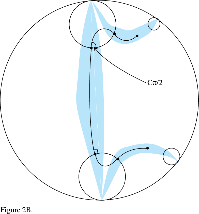 \relabela¡-15pt,-6pt¿ CClose to
\endrelabelbox
\nocolon
\relabela¡-15pt,-6pt¿ CClose to
\endrelabelbox
\nocolon
Lemma 2.5.
The graph is a tree.
Proof.
Suppose not and that there is a path in which runs between vertices without backtracking. This corresponds to some path in which runs from one preimage of the surface to another. We will replace this path by a piecewise geodesic path which will in fact be a long quasi-geodesic. From this it will follow that the path runs between different lifts of , so that it is not a loop in .
Here is the construction: Since it does not involve backtracking, such a path consists of pieces of two types. There are segments which run from horoball to horoball inside a convex hull of some lift of , and segments which run inside the horoball from one lift of to another.
If we see a segment of the first type, we replace it by the common geodesic perpendicular to the pair of horoballs. Notice that this geodesic runs through the centres of both horoballs, which lie in the limit set of this preimage of , so that the geodesic continues to lie inside the convex hull. By construction, such a geodesic makes angle with the horosphere that it meets.
If we see a segment of the path lying inside the horoball connecting different lifts of , we replace it by the geodesic in the horoball between endpoints of the relevant common perpendiculars constructed in the previous paragraph. Note that the distance between such points is enormous, so that this geodesic makes an angle with the horosphere which is very close to . (See Figure 2B.)
Our choices ensure that all the geodesics we construct this way are all very long, moreover, the angle a horoball geodesic piece makes with a convex hull geodesic piece is very close to . This makes the path quasi-geodesic, hence it has distinct endpoints and does not correspond to a closed path in the graph as was required. ∎
Remark\quaAs a first application of this lemma, we note that it implies that if is the centre of some horoball in , then there are no “unexpected” translates of in incident on . That is to say, in the above notation, if , then the first appearance of in our construction places into the image of the orbit at . These are the only preimages of in incident at ; the reason being that any preimage added at a later stage in the construction would give rise to a loop in the graph .
Corollary 2.6.
Suppose that carries some preimage of lying in to another preimage of which lies in .
Then stabilises .
Proof.
We begin by noting that has the following property: Suppose that is the centre of some horoball in , say. This means that there is some translate of , say, in the complex whose limit set contains . We claim that knowing any translate determines the entire complex .
The reason for the claim is this: The translates of which lie in and have limit point at are constructed as the images of the orbit of under some element , which in particular satisfies . By the remark following 2.5, this is exactly the collection of translates in at .
Since lies in , it follows that we can find an element so that , where denotes one of the reference surfaces, ie, either or . (Of course, which one is determined by and which component of that this covers.)
Suppose that is any element of which throws to and the relevant reference surface to . The element stabilises and the reference surface, so it is a power of , that is to say for some integer . We deduce that we can reconstruct the translates of in at as the image of the orbit .
It follows then that we can unambiguously reconstruct the complex outwards using the new set of horoballs that this created, since each such horoball meets a translate of and we may apply the same argument. This proves our claim.
The corollary now follows: If is some element of throwing to and to , then in the notation established in this proof, we may choose to construct the surfaces in incident to and to construct all the surfaces in incident to . From this it follows that maps the surfaces in incident to to the surfaces in incident to . The result follows by building outwards as described above. ∎
We will need to know that has the following property.
Theorem 2.7.
The set has the property that any translate of is either entirely contained inside or is disjoint from it.
The analysis which achieves this is technical and will be deferred to section 2.6
2.3 The subgroup
Define to be the stabiliser in of the complex . We will show that is isomorphic to the fundamental group of a certain –manifold. There is a minor difference between the cases that is the boundary of a twisted -bundle or it is not and so we shall assume henceforth: is not the boundary of a twisted –bundle neighbourhood of a nonorientable surface embedded in .
The minor changes which need to be made in this situation are explained in section 2.5. In fact the only case which really needs to be singled out is the case when is the boundary of a twisted –bundle neighbourhood of a nonorientable surface with one boundary component.
Define this –manifold as follows: Take and glue on a manifold homeomorphic to by identifying with two annuli parallel to contained in . Denote this manifold by . Of course, a manifold homeomorphic to is already embedded inside , however the group corresponds to an immersion of which intuitively comes by attaching one boundary component of to , then spinning the other boundary component around a very long annulus parallel to before attaching to .
The manifold is easily seen to be irreducible and its boundary contains a component of positive genus, so that is Haken. We will show that . To this end we need:
Lemma 2.8.
The complex is simply connected.
Proof.
We note that is constructed as horoballs glued to copies of along thin neighbourhoods of copies of the real line which cover boundary components of . The result then follows from the Seifert–Van Kampen theorem, together with Lemma 2.5. ∎
We may now prove:
Theorem 2.9.
The complex is homeomorphic to , in particular, .
Proof.
The group acts on and Corollary 2.6 shows that
- 1.
acts transitively on the copies of lying in .
- 2.
is a subgroup of .
Taking together and we see that acts transitively on the horoballs of . Moreover, since we assumed that was not the boundary of an –bundle, it follows from results in Chapter of [10], that . Given this we see that is homeomorphic to . Since the complex is simply connected, the result follows. ∎
Remark\quaThe proof shows that this isomorphism identifies the cusp subgroup of with the torus subgroup of in the obvious way.
2.4 Constructing the surface group
We begin with a simple lemma (see also [5], Proposition 2.1):
Lemma 2.10.
Suppose that is an orientable surface with boundary components. Fix some simple closed curve in the boundary of a solid torus which does not bound a disc in . Form a –manifold by identifying all the annuli with disjoint annuli which are all parallel to neighbourhoods of in .
Then contains the fundamental group of a closed orientable surface.
Proof.
By passing to a covering if necessary, it is easy to see that we may assume that meets the disc in the solid torus exactly once transversally.
We form a covering space of in the following way: Take copies of the solid torus and copies of . Any way that we glue these objects together subject to the obvious restrictions coming from the way is glued on to will be a covering space of .
Fix a copy and glue up in any way (subject to being compatible with being a covering) so that each of the boundary components of appears on a different torus. Now glue on a second copy similarly. We claim that this –manifold already contains a closed surface group, which will imply the result, since the remaining part of the covering is constructed by forming HNN construction along curves which are nontrivial in both groups.
We see the claim by noting that all we have done abstractly is take two copies of and identified some component of of one copy with some component of in the other. This manifold has incompressible (though possibly nonorientable) boundary. In particular, it contains a closed surface group, proving the result. ∎
Consider the manifold . Of course, is convex and therefore contractible, so is a , moreover the isomorphism of with is the obvious isomorphism between the boundary torus of and the cusp group of . For future reference we note that is a hyperbolic manifold with convex boundary.
The restriction of the covering map is a map which is a local isometry.
By Theorem 2.7, every translate of is a horoball in which is either contained in or is disjoint from it. It follows that we may excise from and from and define a new map
which continues to be a local isometry. This map induces a covering of boundary tori of degree given by the index of in . Since the curve is mapped 1–1 by this covering, we may extend to a map of the surgered manifolds
Recall that by construction has length more than on , so that using the –theorem [3], we may put negatively curved metrics on both spaces and arrange that the map continues to be a local isometry. We now may prove:
Theorem 2.11.
The map is injective.
Proof.
We begin by observing that although the manifold is not convex, the manifold with the extended metric is convex, since is convex.
Suppose then that the theorem were false and that we could find some element in the kernel of . Since is convex, any such element is freely homotopic to a geodesic in .
The loop is a geodesic in , since is a local isometry. This is a contradiction; if the loop were nullhomotopic, it would lift to be a nullhomotopic geodesic in , a negatively curved complete simply connected manifold and this contradicts the theorem of Hadamard-Cartan. ([8] Theorem 3.1). ∎
Theorem 1.2 now follows:
Theorem 2.12.
The manifold contains the fundamental group of a closed orientable surface
Proof.
Remarks\quaThe reason for using rather than, for example is that there seems to be no a fortiori control over the size of the horoball which embeds into this latter set. Such control is needed in order to apply the theorem.
It also seems worth clarifying why we do not work with the map directly. The reason is that in this setting, to define a map into it is necessary to excise the full preimage in of the horoball . The group stabilises no parabolic fixed points of which lie outside , so there is no way to extend the surgery over those horospheres—and the resulting manifold cannot be made to have convex boundary.
2.5 The case that is the boundary of a twisted –bundle
A variation on the construction above is necessary in the case that that is the twisted –bundle neighbourhood of a nonorientable surface since the stabiliser of is a extension of the surface group . It follows that the manifold as described above is not the correct model for the fundamental group.
The above proof is easily modified if the surface core of the -bundle has at least two boundary components. One performs an analogous construction by gluing a twisted -bundle neighbourhood onto a solid torus. With this proviso, we continue to have and the manifold continues to contain a surface group.
However, if the nonorientable surface core of the –bundle has only a single boundary component, then is double covered by a handlebody. We now sketch how to modify the above proof to deal with this case, and in fact the more general case that is the boundary of the twisted –bundle over a nonorientable surface and that has boundary components.
The construction of is a mild variation on the construction described above. Take “white” copies of the universal covering of , which pass through and meet the boundary of a preimage horoball (chosen to be small as above) in lines which cover the boundary components of . As usual arrange that these copies are very far apart. Similarly, take “black” copies and assume that the black and white complexes are very distant from each other.
Now choose a so that if , then maps this complex of surfaces a very long distance away from itself.
The rest of is constructed much as before save only that we do not allow the identification of white and black surfaces. The group is defined to be the stabiliser of the coloured complex. The proof that the associated graph is a tree is identical. However the complex is a little different and for this we need to modify . The reason for this difference is that the stabiliser of the vertex corresponding to is no longer , but the two-fold extension .
This having been noted, we define the complex to be with two copies of the twisted –bundle over attached in the obvious way. That this complex contains a surface group now can be proved as in 2.10. The rest of the proof is identical.
Remark\quaThough this seems artificial, we note that in the case of a surface with a single boundary component (eg a Seifert surface, see [5]) some sort of operation of this sort is necessary; one cannot tube a surface with a single boundary component to itself.
2.6 The proof of Theorem 2.7
This section is devoted to the proof of the technical result 2.7, which for the reader’s convenience we restate here:
Theorem 2.13.
The set has the property that any translate of is either entirely contained inside or is disjoint from it.
We recall that the thin triangles constant, , for hyperbolic space, is a constant with the property that every point on one side of a geodesic triangle is within a distance of some point on the union of the other two sides. In fact
Lemma 2.14.
There is a constant with the following property. Suppose that and are two points in . Then every point on the geodesic segment connecting to is within a distance of .
Proof.
Throughout this proof we will refer to a translate of the chosen horoball simply as a horoball, and to a translate of as a thick surface.
In 2.5 we constructed a piecewise geodesic, in with endpoints and The geodesic segments in this path are of two types. The first type is a geodesic segment in a thick surface. The second type is a geodesic segment in a horoball. The endpoints of these segments, other than and are on the intersection of some thick surface with some horoball. A segment contained in a thick surface is orthogonal to the boundary of any horoballs at its endpoints. The same is not generally true for segments in horoballs.
In 2.5 every segment in a horoball was long (length at least ) and therefore almost orthogonal to the boundary of the horoball at its endpoints. In the present situation, this fails precisely when or is in a horoball. Thus is a piecewise geodesic, and all the segments, except possibly the first and last, have length at least The angle between two adjacent segments is very close to except possibly for the first and last angles.
Using the above properties of it is well known that the geodesic with endpoints lies within of . We sketch this: Let be the first geodesic segment and the last segment of . The subpath of excluding the first and last segment consists of segments all of length at least and with all angles between adjacent segments within the range Let be the geodesic with endpoints and . Then every point of is within of Now consider the geodesic path Let be the geodesic with the same endpoints as Then is a geodesic quadrilateral.
By dividing this into two geodesic triangles, we see that every point on is within of Now every point of is within of a point of Hence every point of is within of which is contained in ∎
Lemma 2.15.
There is a constant such that if is a geodesic tetrahedron with all four vertices in then every point of is within a distance of .
Proof.
We prove below that every point in the boundary of is within a distance of some point in Given a point in the interior of there is a geodesic triangle with edges contained in the boundary of and which contains Hence is within a distance of of some point in the boundary of Therefore within of some point of
Let be a face of Thus is a geodesic hyperbolic triangle with vertices contained in Suppose that is a point in There is a geodesic segment, in containing and with one endpoint and the other endpoint, on Let be a point of closest to By Lemma 2.14, Moreover, is within of The points are both in . With another application of Lemma 2.14, we see that every point on is within a distance of Since is in every point on is within of Therefore is within a distance of a point within a distance of Hence ∎
Lemma 2.16.
Suppose that is an increasing sequence of compact subsets of The convex hull, of is the closure of
Proof.
It is clear that contains the convex hull of Since is closed, it contains the closure of Moreover, is an increasing sequence of convex sets and it follows that is convex. Hence the closure is convex. Thus is contained in this closure.∎
Proposition 2.17.
Every point in the convex hull of is within a distance of
Proof.
The convex hull of a compact subset, of is equal to the union of all geodesic tetrahedra having all four vertices in (we allow degenerate tetrahedra where some of the vertices coincide).
Proof of 2.7.
By our initial careful choices of , any translate of not lying in is very far from . However, by 2.17, is very close to , whence the result. ∎
The authors thank A W Reid for carefully reading an early version of this paper and the referee for several useful comments.
Both authors are supported in part by the NSF.
References
- [1] F Bonahon, Bouts des variétés hyperboliques de dimension 3, Ann. of Math. 124 (1986) 71–158
- [2] H Bass, J Morgan, The Smith Conjecture, Academic Press (1984)
- [3] S Bleiler, C Hodgson, Spherical Space Forms and Dehn Fillings, Topology, 3 (1996) 809–833
- [4] D Canary, D B A Epstein, P Green, Notes on notes of Thurston, from “Analytic and Geometric Aspects of Hyperbolic Space”, (D B A Epstein, editor) LMS Lecture Notes, vol. 111 (1987)
- [5] D Cooper, D D Long, Virtually Haken surgery on knots, J. Diff Geometry, 52 (1999) 173–187
- [6] D Cooper, D D Long, A W Reid, Essential closed surfaces in bounded –manifolds, J. Amer. Math. Soc. 10 (1997) 553–564
- [7] M Culler, C McA Gordon, J Luecke, P B Shalen, Dehn surgery on knots, Ann. of Math. 125 (1987) 237–300
- [8] M do Carmo, Riemannian manifolds, Birkhauser (1992)
- [9] S Fenley, Quasifuchsian Seifert Surfaces, Math. Zeit. 228 (1998) 221–227
- [10] J Hempel, 3–Manifolds, Annals of Math Studies, 86, Princeton University Press (1976)
- [11] W Jaco, Lectures on Three-Manifold Topology, CBMS series 43 (1977)
- [12] T Li, Immersed essential surfaces in hyperbolic 3–manifolds, Comm. Anal. Geom. (to appear)
- [13] W P Thurston, The geometry and topology of 3–manifolds, Princeton University Press