\newarrowhead

+¿ \rMapsto\leftmapsto\downmapsto\upmapsto\newarrowTo —-¿ \newarrowMapsto ——¿ \newarrowNoto —– \newarrowInto ¿—¿ \newarrowOnto —-¿¿ \newarrowIso ¿—¿¿ \newarrowInclus C—¿ \newarrowEqual ===== \newarrowDash dashdashdashdashdash \newarrowDashto dashdashdashdash¿

Spin Borromean Surgeries

Gwénaël Massuyeau Address: Laboratoire de Mathématiques de Nantes
UMR 6629 CNRS/Université de Nantes
2, rue de la Houssinière
BP 92208
44322 Nantes Cedex 03
France Email address: massuyea@math.univ-nantes.fr

Date: October 20, 2000 and, in revised form, March 26, 2002.

Abstract.

In 1986, Matveev defined the notion of Borromean surgery for closed oriented $3$ -manifolds and showed that the equivalence relation generated by this move is characterized by the pair (first betti number, linking form up to isomorphism).
We explain how this extends for $3$ -manifolds with spin structure if we replace the linking form by the quadratic form defined by the spin structure. We then show that the equivalence relation among closed spin $3$ -manifolds generated by spin Borromean surgeries is characterized by the triple (first betti number, linking form up to isomorphism, Rochlin invariant modulo $8$ ).

Key words and phrases:

3-manifolds, finite type invariants, spin structures, Y-graphs

2000 Mathematics Subject Classification

57M27, 57R15

Introduction

The notion of Borromean surgery was introduced by Matveev in [Ma] as an example of what he called a $\mathcal{V}$ -surgery. Since then, this transformation has become the elementary move of Goussarov-Habiro finite type invariants theory for oriented $3$ -manifolds ([Ha], [Go], [GGP]). Matveev showed that the equivalence relation, among closed oriented $3$ -manifolds, generated by Borromean surgery is characterized by the pair:

(\beta_{1}(M),\textrm{ isomorphism class of }\lambda_{M}),

where $\beta_{1}(M)$ is the first Betti number of a $3$ -manifold $M$ and

TH_{1}(M;\mathbf{Z})\otimes TH_{1}(M;\mathbf{Z})\rTo^{\lambda_{M}}\mathbf{Q}/\mathbf{Z}

is its torsion linking form. This result gives a characterization of degree $0$ invariants in Goussarov-Habiro theory for closed oriented $3$ -manifolds.

As mentioned by Habiro and Goussarov, their finite type invariants theory (in short: “FTI theory”) makes sense also for $3$ -manifolds with spin structure because Borromean surgeries work well with spin structures (see §2). So, the question is: what is the “spin” analogue of Matveev’s theorem?
For each closed spin $3$ -manifold $(M,\sigma)$ , a quadratic form

TH_{1}(M;\mathbf{Z})\rTo^{\phi_{M,\sigma}}\mathbf{Q}/\mathbf{Z}

can be defined by many ways (see [LL], [MS], and also [Tu], [Gi]). The bilinear form associated to $\phi_{M,\sigma}$ is $\lambda_{M}$ . Its Gauss-Brown invariant is equal to $-R_{M}(\sigma)$ modulo $8$ , where

Spin(M)\rTo^{R_{M}}\mathbf{Z}_{16}

is the Rochlin function of $M$ , sending a spin structure $\sigma$ of $M$ to the modulo $16$ signature of a spin $4$ -manifold which spin-bounds $(M,\sigma)$ . The main result of this paper is the following refinement of Matveev’s theorem:

Theorem 1.

Let $(M,\sigma)$ and $(M^{\prime},\sigma^{\prime})$ be connected closed spin $3$ -manifolds.
Then, the following assertions are equivalent:

(1)

$(M,\sigma)$ and $(M^{\prime},\sigma^{\prime})$ can be obtained from one another by spin Borromean surgeries,
(2)

there exists a homology isomorphism $f:H_{1}(M;\mathbf{Z})\rTo H_{1}(M^{\prime};\mathbf{Z})$ such that:

$\phi_{M,\sigma}=\phi_{M^{\prime},\sigma^{\prime}}\circ f|_{TH_{1}(M;\mathbf{Z})},$
(3)

$R_{M}(\sigma)=R_{M^{\prime}}(\sigma^{\prime})$ modulo $8$ and there exists a homology isomorphism $f:H_{1}(M;\mathbf{Z})\rTo H_{1}(M^{\prime};\mathbf{Z})$ such that:

$\lambda_{M}=\lambda_{M^{\prime}}\circ f|_{TH_{1}(M;\mathbf{Z})}.$

The equivalence between assertions 2 and 3 will be the topological statement of an algebraic fact: a nondegenerate quadratic form on a finite Abelian group is determined, up to isomorphism, by its associated bilinear form and its Gauss-Brown invariant.

In §1 we recall Matveev’s notion of $\mathcal{V}$ -surgery. With this background, we then recall the definition of Borromean surgery, and give equivalent descriptions of other authors.
In §2, we clarify how all of these notions have to be understood in the spin case: in particular, spin Borromean surgeries are introduced. As a motivation to Theorem 1, FTI for spin $3$ -manifolds, in the sense of Habiro and Goussarov, are then defined: the Rochlin invariant is shown to be a finite type degree $1$ invariant. It should be mentioned that Cochran and Melvin have proposed a different FTI theory in [CM], and have also refined their theory to the case of spin manifolds.
§3 is of an algebraic nature. We recall some definitions and results about quadratic forms on finite Abelian groups. We also prove the above mentioned algebraic fact: the proof makes use of Kawauchi-Kojima classification of linking pairings.
§4 is the topological cousin of the former: we review the quadratic form $\phi_{M,\sigma}$ . Starting from Turaev $4$ -dimensional definition in [Tu], we then give an intrinsic definition for $\phi_{M,\sigma}$ (no reference to dimension $4$ ).
§5 is devoted to the proof of Theorem 1. It goes as a refinement of the original proof by Matveev for the “unspun” case. Last section will give some of its applications.

Acknowledgments

The author wants to thank his advisor Pr. Christian Blanchet who supervised this work, and Florian Deloup for conversations regarding quadratic forms. He is also indebted to Félicie Pastore for correcting his written english.

1. Borromean surgeries and equivalent moves

First of all, we want to recall the unifying idea of $\mathcal{V}$ -surgery by Matveev in [Ma]. This will allow us to have a more conceptual view of Borromean surgeries.

1.1. Review of Matveev $\mathcal{V}$ -surgeries

We begin with some general definitions.

Definition 1.

A Matveev triple is a triple of oriented $3$ -manifolds:

(1)

\mathcal{V}=(V,V_{1},V_{2}),

where $V$ is closed and is the union of $-V_{1}$ and $V_{2}$ along their common boundary $\partial V_{1}=\partial V_{2}$ , as depicted in Figure 1.
The triple $(-V,V_{2},V_{1})$ is called the inverse of $\mathcal{V}$ and is denoted by $\mathcal{V}^{-1}$ .

Refer to caption — Figure 1. What will be removed and what will be glued during the surgery.

Let now $M$ be a closed oriented $3$ -manifold and let $j:V_{1}\rTo M$ be an orientation-preserving embedding. Form the following closed oriented $3$ -manifold:

(2)

M^{\prime}=M\setminus int\left(j(V_{1})\right)\cup_{j|_{\partial}}V_{2}.

Definition 2.

With the above notations, $M^{\prime}$ is said to be obtained from $M$ by $\mathcal{V}$ -surgery along $j$ .

Note that if $k$ denotes the embedding of $V_{2}$ in $M^{\prime}$ , then $M$ is obtained from $M^{\prime}$ by $\mathcal{V}^{-1}$ -surgery along $k$ .

Definition 3.

Two Matveev triples $\mathcal{V}$ and $\mathcal{V^{\prime}}$ are said to be equivalent if there exists an orientation-preserving diffeomorphism from $V$ to $V^{\prime}$ sending $-V_{1}$ to $-V^{\prime}_{1}$ , and $V_{2}$ to $V^{\prime}_{2}$ .

Note that, if the triples $\mathcal{V}$ and $\mathcal{V^{\prime}}$ are equivalent, then they have the same surgery effect.

Example 1.

Let $\Sigma_{g}$ denote the genus $g$ closed oriented surface and let $H_{g}$ be the genus $g$ oriented handlebody. Then, each orientation-preserving diffeomorphism $f:\Sigma_{g}\rTo\Sigma_{g}$ leads to a triple:

\mathcal{V}_{f}:=\left((-H_{g})\cup_{f}H_{g},H_{g},H_{g}\right).

A $\mathcal{V}_{f}$ -surgery amounts to “twist” an embedded genus $g$ handlebody by $f$ . For instance, from the standard genus one Heegaard decomposition of $\mathbf{S}^{3}$ , integral Dehn surgery is recovered.

1.2. Review of Borromean surgeries

The original Matveev’s point of view was:

Definition 4.

A Borromean surgery is a $\mathcal{B}$ -surgery with:

\mathcal{B}=\left(B:=(-B_{1})\cup B_{2},B_{1},B_{2}\right),

where the “halves” $B_{1}$ and $B_{2}$ are obtained from the genus $3$ handlebody by surgery on three-component framed links as shown in Figure¹¹ 1 Blackboard framing convention is used. 2.

We now recall Goussarov’s notion of $Y$ -surgery in [Go]. This move is equivalent to the $A_{1}$ -move of Habiro in [Ha].

Definition 5.

A $Y$ -graph $G$ in a closed oriented $3$ -manifold $M$ is an (unoriented) embedding of the surface drawn in Figure 3, together with its decomposition between leaves, edges and node.
The closed oriented $3$ -manifold obtained from $M$ by $Y$ -surgery along $G$ is:

M_{G}:=(M\setminus int(N(G)))\cup(H_{3})_{L},

where $N(G)\cong_{+}H_{3}$ is a regular neighbourhood of $G$ in $M$ , and $(H_{3})_{L}$ is the surgered handlebody on the six-component link $L$ drawn on Figure 4.
We call $Y$ -equivalence the equivalence relation among closed oriented $3$ -manifolds generated by orientation-preserving diffeomorphisms and $Y$ -surgeries.

Note that a $Y$ -surgery is a $\mathcal{Y}$ -surgery if we call $\mathcal{Y}$ the triple:

\mathcal{Y}=\left(Y:=(-H_{3})\cup(H_{3})_{L},H_{3},(H_{3})_{L}\right),

the corresponding $Y$ -graph gives the place where the $\mathcal{Y}$ -surgery must be performed.

Lemma 1.

The Matveev triples $\mathcal{B}$ and $\mathcal{Y}$ are equivalent. Thus, Borromean surgery is equivalent to $Y$ -surgery.

Proof.

We will show that both of the triples $\mathcal{B}$ and $\mathcal{Y}$ are equivalent to a triple $\mathcal{V}_{h}$ , defined by an orientation-preserving diffeomorphism $h:\Sigma_{3}\rTo\Sigma_{3}$ .
We start with the “half” $(H_{3})_{L}$ of Figure 4: handle-sliding of each node-component over the corresponding leaf-component, followed by some isotopies of framed links gives Figure 5, where only part of the link is drawn.

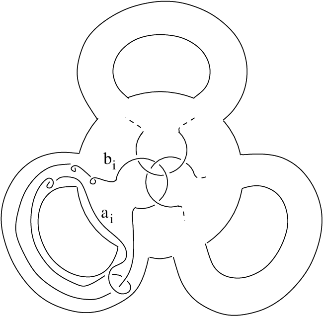
Up to a $(+1)$ -framing correction, the three depicted components $a_{i}$ can be normally pushed off at once towards the boundary: we obtain three disjoint curves $\alpha_{i}$ on $\partial H_{3}$ . Note that during this push-off, none of the three components $b_{i}$ is intersected. Then, the components $b_{i}$ can also be pushed off so that the framing correction is now $-1$ : the result is a family of three disjoint curves $\beta_{i}$ . After a convenient isotopy of the handles, the curves $\alpha_{i}$ and $\beta_{i}$ can be depicted as on Figure 6.

We define $h:=h_{b}^{-1}\circ h_{a}$ , where $h_{a}$ and $h_{b}$ are the following composites of (commuting) Dehn twists:

h_{a}=\prod_{i=1}^{3}\tau_{\alpha_{i}}\hskip 10.00002pt\textrm{and}\hskip 10.00002pth_{b}=\prod_{i=1}^{3}\tau_{\beta_{i}}.

According to the Lickorish trick [Li, proof of Theorem 2], a $\mathcal{Y}$ -surgery is therefore equivalent to a $\mathcal{V}_{h}$ -surgery.

On the other hand, from Figure 2, we deduce that a $\mathcal{B}$ -surgery is equivalent to a $\mathcal{V}_{h^{\prime}}$ -surgery where $h^{\prime}:=h_{b}\circ h_{a}^{-1}$ . Let $m_{i}$ denote the meridian of the $i^{e}$ handle of $H_{3}$ , for $i=1,2,3$ . Then, the equation:

(3)

k^{-1}=k\circ\prod_{i=1}^{3}\tau_{m_{i}}^{2}

holds for both $h_{a}$ and $h_{b}$ so that $h=h^{\prime}$ . ∎

Remark 1 (Fundamental remark).

Note that, in the proof of Lemma 1, the curve $\alpha_{i}$ is homologous in the surface $\Sigma_{3}$ to the corresponding curve $\beta_{i}$ (look at Figure 6). As a consequence, the diffeomorphism $h:\Sigma_{3}\rTo\Sigma_{3}$ belongs to the Torelli group. In the sequel, we will call $h$ the Borromean diffeomorphism.

In order to have a complete understanding of these equivalent triples $\mathcal{B}$ , $\mathcal{Y}$ or $\mathcal{V}_{h}$ , it remains to recognize their underlying closed $3$ -manifolds.

Lemma 2.

The closed $3$ -manifolds $B$ and $Y$ , respectively defined by the triples $\mathcal{B}$ and $\mathcal{Y}$ , are both homeomorphic to the $3$ -torus $\mathbf{S}^{1}\times\mathbf{S}^{1}\times\mathbf{S}^{1}$ .

Proof.

According to Lemma 1, $B$ and $Y$ are diffeomorphic. Let us identify $Y$ . Recall that $Y$ was defined as:

(4)

Y=(-H_{3})\cup(H_{3})_{L}.

Write $L$ as $L_{a}\ \dot{\cup}\ L_{b}$ where $L_{a}$ (resp. $L_{b}$ ) is the sublink containing the leaf(resp. node)-components. Note that $L_{b}$ can be isotoped in $Y\setminus L_{a}$ to some Borromean rings contained in a $3$ -ball disjoint from $L_{a}$ : make $L_{b}$ leave the handlebody where it was lying, towards the handlebody with the minus sign in (4). So $Y$ is obtained from $(-H_{3})\cup(H_{3})_{L_{a}}$ by surgery on some Borromean rings contained in a little $3$ -ball. The lemma then follows from the fact that the latter is nothing but $\mathbf{S}^{3}$ . ∎

2. Spin Borromean surgeries

We now go into the world of spin $3$ -manifolds. We refer to [Ki, Chapter IV] for an introduction to spin structures. As a warming up, we recall a few facts in the next subsection.

2.1. Glueing of spin structures

Let $n\geq 2$ , and let $M$ be a compact smooth oriented $n$ -manifold endowed with a Riemannian metric. Its bundle of oriented orthonormal frames will be denoted by $FM$ : it is a principal $SO(n)$ -bundle with total space $E(FM)$ and with projection $p$ .
Recall that if $M$ is spinnable, $Spin(M)$ can be thought of as:

Spin(M)=\left\{\sigma\in H^{1}\left(E(FM);\mathbf{Z}_{2}\right)\ :\ \sigma|_{\textrm{fiber}}\neq 0\in H^{1}\left(SO(n);\mathbf{Z}_{2}\right)\right\},

and is essentially independant of the metric. The set $Spin(M)$ is then an affine space over $H^{1}(M;\mathbf{Z}_{2})$ , the action being defined by:

\forall x\in H^{1}(M;\mathbf{Z}_{2}),\ \forall\sigma\in Spin(M),\ x\cdot\sigma:=\sigma+p^{*}(x).

Lemma 3.

For $i=1,2$ , let $M_{i}$ be a compact smooth oriented $n$ -manifold and let $S_{i}$ be a submanifold of $\partial M_{i}$ with orientation induced by $M_{i}$ . Let also $f:S_{2}\rTo S_{1}$ be an orientation-reversing diffeomorphism and let $M=M_{1}\cup_{f}M_{2}$ .
Assume that $M_{1}$ and $M_{2}$ are spinnable, that $S_{2}$ is connected, and that the set:

J=\left\{(\sigma_{1},\sigma_{2})\in Spin(M_{1})\times Spin(M_{2})\ :\ f^{*}\left(-\sigma_{1}|_{S_{1}}\right)=\sigma_{2}|_{S_{2}}\right\}

is not empty. Then, $M$ is spinnable and the restriction map:

\left\{\begin{array}[]{rrcl}Spin(M)&\rTo^{r}&Spin(M_{1})\times Spin(M_{2})\\ \sigma&\rMapsto&\left(\sigma|_{M_{1}},\sigma|_{M_{2}}\right),\end{array}\right.

is injective with $J$ as image.

Proof.

For $i=1$ or $2$ , let $F^{+}S_{i}$ be the principal $SO(n)$ -bundle derived from $FS_{i}$ and the inclusion of groups: {diagram} We still denote by $g$ the canonical map from $FS_{i}$ to $F^{+}S_{i}$ . Then, {diagram} is an isomorphism. The bundle $F^{+}S_{i}$ can be identified with $FM_{i}|_{S_{i}}$ . In particular, there is an inclusion map $k_{i}:E\left(F^{+}S_{i}\right)\rInclus E(FM_{i})$ .

Moreover, the diffeomorphism $f$ induces a further identification: {diagram} such that the total space $E(FM)$ is homeomorphic to the glueing:

E(FM_{1})\cup_{k_{1}fk_{2}^{-1}}E(FM_{2}).

We denote by $j_{i}$ the corresponding inclusion of $E(FM_{i})$ into $E(FM)$ . But now, by the Mayer-Vietoris sequence, we have: {diagram} Note that $g^{*}\circ(k_{1}\circ f)^{*}$ sends each $\sigma_{1}\in Spin(M_{1})$ to $f^{*}(-\sigma_{1}|_{S_{1}})$ , while $g^{*}\circ k_{2}^{*}$ sends each $\sigma_{2}\in Spin(M_{2})$ to $\sigma_{2}|_{S_{2}}$ . Note also that, since $S_{2}$ is connected, the map $(j_{1}^{*},j_{2}^{*})$ is injective. The whole lemma then follows from these two remarks and from the exactness of the Mayer-Vietoris sequence. ∎

Definition 6.

With the notations and hypothesis of Lemma 3, for each $(\sigma_{1},\sigma_{2})\in J$ , the unique spin structure of $M$ sent by $r$ to $(\sigma_{1},\sigma_{2})$ is called the glueing of the spin structures $\sigma_{1}$ and $\sigma_{2}$ , and is denoted by $\sigma_{1}\cup\sigma_{2}$ .

2.2. Spin $\mathcal{V}$ -surgeries

In some cases, a Matveev $\mathcal{V}$ -surgery, whose definition has been recalled in §1.1, makes sense for spin $3$ -manifolds.

Definition 7.

A Matveev triple $\mathcal{V}=(V,V_{1},V_{2})$ is said to be spin-admissible, if $\partial V_{1}=\partial V_{2}$ is connected, and if the maps:

H^{1}(V;\mathbf{Z}_{2})\rTo H^{1}(V_{1};\mathbf{Z}_{2})\hskip 10.00002pt\textrm{and}\hskip 10.00002ptH^{1}(V;\mathbf{Z}_{2})\rTo H^{1}(V_{2};\mathbf{Z}_{2}),

induced by inclusions, are isomorphisms.

Suppose now that $\mathcal{V}$ is a spin-admissible triple. Note that the restriction maps: {diagram} are then bijective. Let also $M$ be a closed oriented $3$ -manifold and let $j:V_{1}\rTo M$ be an orientation-preserving embedding. As in §1.1, we denote by $M^{\prime}$ the result of the $\mathcal{V}$ -surgery along $j$ , and we want to define a canonical bijection: {diagram} First, the embedding $j$ allows us to define the following map:

\left\{\begin{array}[]{rrcl}Spin(M)&\rTo^{\Upsilon_{j,\mathcal{V}}}&Spin(V)\\ \sigma&\rMapsto&r_{1}^{-1}(-j^{*}(\sigma)).\end{array}\right.

From formula (2) and from Definition 6, we can define $\Theta_{j,\mathcal{V}}(\sigma)$ as the following glueing:

\Theta_{j,\mathcal{V}}(\sigma):=\sigma|_{M\setminus int\left(j(V_{1})\right)}\ \cup\ r_{2}\left(\Upsilon_{j,\mathcal{V}}(\sigma)\right).

The inverse of $\Theta_{j,\mathcal{V}}$ is $\Theta_{k,\mathcal{V}^{-1}}$ , where $k$ denotes the embedding of $V_{2}$ in $M^{\prime}$ .

Definition 8.

With the above notations, the spin manifold $\left(M^{\prime},\Theta_{j,\mathcal{V}}(\sigma)\right)$ is said to be obtained from $(M,\sigma)$ by spin $\mathcal{V}$ -surgery along $j$ .

Example 2.

Let $f:\Sigma_{g}\rTo\Sigma_{g}$ be an orientation-preserving diffeomorphism. Denote by $K$ the lagrangian subspace of $H_{1}(\Sigma_{g};\mathbf{Z}_{2})$ span by the meridians. Then, as can be easily verified, the triple $\mathcal{V}_{f}$ of Example 1 is spin-admissible if and only if $f_{*}(K)=K$ . For instance, this condition is satisfied when $f$ belongs to the Torelli modulo $2$ group.

Lemma 4.

In the particular case of Example 2, that is when $\mathcal{V}=\mathcal{V}_{f}$ with $f_{*}(K)=K$ , then for each $\sigma\in Spin(M)$ , $\Theta_{j,\mathcal{V}}(\sigma)$ is the unique spin structure of $M^{\prime}$ extending $\sigma|_{M\setminus int\left(j(V_{1})\right)}$ .

Proof.

In that case, $V_{2}$ is a handlebody and so $H^{1}\left(M^{\prime},M\setminus int\left(j(V_{1})\right);\mathbf{Z}_{2}\right)$ is zero. Therefore, the restriction map $Spin(M^{\prime})\rTo Spin(M\setminus int(j(V_{1})))$ is injective. ∎

2.3. Definition of $Y^{s}$ -surgeries

From Lemma 1 and from Remark 1 above, we have learnt that both of the triples $\mathcal{B}$ and $\mathcal{Y}$ are equivalent to the triple $\mathcal{V}_{h}$ where $h$ is the Borromean diffeomorphism which belongs to the Torelli group. So, by Example 2, they are spin-admissible and the following definition makes sense:

Definition 9.

A $Y^{s}$ -surgery, or equivalently a spin Borromean surgery, is the surgery move among closed spin $3$ -manifolds defined equivalently by the triples $\mathcal{Y}$ or $\mathcal{B}$ . We call $Y^{s}$ -equivalence the equivalence relation among them generated by spin diffeomorphisms and $Y^{s}$ -surgeries.

Let $(M,\sigma)$ be a closed spin $3$ -manifold and let $G$ be a $Y$ -graph in $M$ . The $Y^{s}$ -surgery along $G$ gives a new spin manifold which will be denoted by:

(M_{G},\sigma_{G}).

Let $j:H_{3}\rTo N(G)$ be an embedding of the genus 3 handlebody onto a regular neighbourhood of $G$ in $M$ . Then,

(5)

M_{G}\cong M\setminus int\left(N(G)\right)\cup_{j|_{\partial}\circ h}H_{3},

and according to Lemma 4, $\sigma_{G}$ is the unique spin structure of $M_{G}$ extending $\sigma|_{M\setminus int\left(N(G)\right)}$ .

2.4. Goussarov-Habiro FTI theory for spin $3$ -manifolds

Lemma 5.

Let $(M,\sigma)$ be a closed spin $3$ -manifold and let $G$ and $H$ be disjoint $Y$ -graphs in $M$ . Then, up to diffeomorphism of manifolds with spin structure,

\left((M_{G})_{H},(\sigma_{G})_{H}\right)=\left((M_{H})_{G},(\sigma_{H})_{G}\right).

Proof.

The equality $(M_{G})_{H}=(M_{H})_{G}$ is obvious. By construction, both of $(\sigma_{G})_{H}$ and $(\sigma_{H})_{G}$ are extensions of $\sigma|_{M\setminus\left(N(G)\cup N(H)\right)}$ . The lemma then follows from the fact that the restriction map: {diagram} is injective since the relative cohomology group $H^{1}\left((M_{G})_{H},M\setminus\left(N(G)\cup N(H)\right);\mathbf{Z}_{2}\right)$ is zero. ∎

Let $S=\{G_{1},\dots,G_{s}\}$ be a family of disjoint $Y$ -graphs in a closed $3$ -manifold $M$ with spin structure $\sigma$ . Lemma 5 says that $Y^{s}$ -surgery along the family $S$ is well-defined. We denote the result by $(M_{S},\sigma_{S})$ . Following Habiro and Goussarov definition of a finite type invariant ([Ha], [Go]), we can now define:

Definition 10.

Let $A$ be an Abelian group and let $\lambda$ be an $A$ -valued invariant of $3$ -manifolds with spin structure. Then, $\lambda$ is an invariant of degree at most $n$ if for any closed spin $3$ -manifold $(M,\sigma)$ and any family $S$ of at least $n+1$ $Y$ -graphs in $M$ , the following identity holds:

(6)

\sum_{S^{\prime}\subset S}\lambda(M_{S^{\prime}},\sigma_{S^{\prime}})=0\in A,

where the sum is taken over all subfamilies $S^{\prime}$ of $S$ . Moreover, $\lambda$ is of degree $n$ if it is of degree at most $n$ , but is not of degree at most $n-1$ .

Remark 2.

Note that the degree $0$ invariants are precisely those invariants which are constant on each $Y^{s}$ -equivalence class. So, the refined Matveev theorem will quantify how powerful they can be.

The next subsection will provide us some examples of invariants which are finite type in the sense of Definition 10.

2.5. Rochlin invariant under $Y^{s}$ -surgery

Proposition 1.

Let $(M,\sigma)$ be a closed spin $3$ -manifold, and let $G$ be a $Y$ -graph in $M$ . Then, the following formula holds:

R_{M_{G}}(\sigma_{G})=R_{M}(\sigma)+R_{\mathbf{S}^{1}\times\mathbf{S}^{1}\times\mathbf{S}^{1}}\left(\Upsilon_{G}(\sigma)\right)\in\mathbf{Z}_{16},

where the map $\Upsilon_{G}:Spin(M)\rTo Spin(\mathbf{S}^{1}\times\mathbf{S}^{1}\times\mathbf{S}^{1})$ , induced by the $\mathcal{Y}$ -surgery along $G$ , has been defined in §2.2.

Proof.

According to Lemma 2, we can think of the $3$ -torus as:

(7)

\mathbf{S}^{1}\times\mathbf{S}^{1}\times\mathbf{S}^{1}=(-H_{3})\cup_{h}H_{3}.

The surgered manifold $M_{G}$ will be thought of concretely as in (5).
Pick a spin $4$ -manifold $W$ spin-bounded by $(M,\sigma)$ , and a spin $4$ -manifold $H$ spin-bounded by the $3$ -torus with $\Upsilon_{G}(\sigma)$ as a spin structure. Glue the “generalized” handle $H$ to $W$ along the first handlebody of the $3$ -torus in decomposition (7), using $j$ as glue. We obtain a $4$ -manifold $W^{\prime}$ . Orient $W^{\prime}$ coherently with $H$ and $W$ , and then give to $W^{\prime}$ the spin structure obtained by glueing those of $H$ and $W$ (see Definition 6). It follows from definitions that the spin-boundary of $W^{\prime}$ is $(M_{G},\sigma_{G})$ .
According to Wall theorem on non-additivity of the signature (see [Wa3]), we have:

(8)

sgn(W^{\prime})=sgn(W)+sgn(H)-\textrm{ correcting term}.

The involved correcting term is the signature of a real bilinear symmetric form explicitely described by Wall. It is defined by means of the intersection form in $\Sigma_{3}$ , with domain:

V=\frac{A\cap(B+C)}{A\cap B+A\cap C},

where $A$ , $B$ , $C$ are subspaces of $H_{1}(\Sigma_{3};\mathbf{R})$ defined to be respectively the kernels of: {diagram} No matter who is $A$ , since the Borromean diffeomorphism $h$ lies in the Torelli group, we certainly have $B=C$ . The space $V$ then vanishes and so does the correcting term. The announced equality then follows by taking equation (8) modulo $16$ . ∎

Corollary 1.

The Rochlin invariant is a degree $1$ invariant of closed spin $3$ -manifolds for Goussarov-Habiro theory, and its modulo $8$ reduction is of degree $0$ .

Remark 3.

In Cochran-Melvin theory, the Rochlin invariant is a degree $3$ finite type invariant (see [CM, Prop. 6.2]).

Proof of Corollary 1.

Last statement is clear from Proposition 1 and from the fact that the Rochlin function of the $3$ -torus takes values in $\{0,8\}\subset\mathbf{Z}_{16}$ . Let us show that the Rochlin invariant is at most of degree $1$ . Take a closed spin $3$ -manifold $(M,\sigma)$ and two disjoint $Y$ -graphs $G$ and $H$ in $M$ . According to Proposition 1, in order to show that:

(9)

R_{M}(\sigma)-R_{M_{G}}(\sigma_{G})-R_{M_{H}}(\sigma_{H})+R_{M_{G,H}}(\sigma_{G,H})=0,

it suffices to show that:

(10)

\Upsilon_{G}(\sigma)=\Upsilon_{G}(\sigma_{H})\in Spin(\mathbf{S}^{1}\times\mathbf{S}^{1}\times\mathbf{S}^{1}),

where the left $\Upsilon_{G}$ is defined by $G\subset M$ and the right $\Upsilon_{G}$ is defined by $G\subset M_{H}$ . But this follows from definition of the maps $\Upsilon_{G}$ and from the fact that $\sigma_{H}$ extends $\sigma|_{M\setminus N(H)}$ .
It remains to show that the Rochlin invariant is not of degree $0$ (and so it will be “exactly” of degree $1$ ). For instance, all of the spin structures of the $3$ -torus are related one to another by $Y^{s}$ -surgeries (Cf Example 3 below) and so are not distinguished one to another by degree $0$ invariants. But Rochlin distinguishes one of them from the others. ∎

2.6. $Y^{s}$ -surgeries through surgery presentations on $\mathbf{S}^{3}$

We first fix some notations.

We call $V_{L}$ the $3$ -manifold obtained from $\mathbf{S}^{3}$ by surgery along a ordered oriented framed link $L=(L_{1},\dots,L_{l})$ of length $l$ , and $W_{L}$ the corresponding $4$ -manifold obtained from $\mathbf{B}^{4}$ by attaching $2$ -handles and sometimes called the trace of the surgery. Let also $B_{L}=(b_{ij})_{i,j=1,\dots,l}$ be the linking matrix of $L$ .
Recall that $H_{2}(W_{L};\mathbf{Z})$ is free Abelian of rank $l$ . For each $i=1,\dots,l$ , choose a Seifert surface of $L_{i}$ in $\mathbf{S}^{3}$ and push it off into the interior of $\mathbf{B}^{4}$ : denote the result by $P_{i}$ . Then, glue $P_{i}$ to the core of the $i^{e}$ $2$ -handle to obtain a closed surface $S_{i}$ . A basis of $H_{2}(W_{L};\mathbf{Z})$ is then given by $([S_{1}],\dots,[S_{l}])$ .

We now recall a nice combinatorial way to describe spin structures of $V_{L}$ .

This is by means of the so-called “characteristic solutions of $B_{L}$ ” or, equivalently, “characteristic sublinks of $L$ ”.
A vector $s\in(\mathbf{Z}_{2})^{l}$ or, equivalently, the sublink of $L$ containing the components $L_{i}$ such that $s_{i}=1$ , are said to be characteristic if the following equation is satisfied:

(11)

\forall i=1,\dots,l\ ,\hskip 10.00002pt\sum_{j=1}^{l}b_{ij}\cdot s_{j}=b_{ii}\in\mathbf{Z}_{2}.

We denote by $\mathcal{S}_{L}$ the subset of $(\mathbf{Z}_{2})^{l}$ comprising the characteristic solutions of $B_{L}$ . There is a bijection: {diagram} which is defined by the following composition: {diagram} where $o$ sends any $\sigma\in Spin(V_{L})$ to the obstruction to extend $\sigma$ to the whole of $W_{L}$ , $P$ is the Poincaré duality isomorphism and the last map is defined by the basis $([S_{1}],\dots,[S_{l}])$ . With this combinatorial description, Kirby theorem can be refined to closed spin $3$ -manifolds (see [Bl]).
The following lemma, more general than needed, will allow us to enunciate in those terms the effect of a $Y^{s}$ -surgery.

Lemma 6.

Let $L\cup K$ be the ordered union of two ordered oriented framed links in $\mathbf{S}^{3}$ and let $H\subset S^{3}$ be an embedded handlebody such that $K$ is contained in the interior of $H$ , $L$ is disjoint from $H$ , and $H_{K}$ is a $\mathbf{Z}_{2}$ -homology handlebody.

Suppose that $\sigma\in Spin\left(V_{L\cup K}\right)$ is represented by a characteristic solution $s\in(\mathbf{Z}_{2})^{l+k}$ of $B_{L\cup K}$ satisfying the following two properties:

(1)

$(s_{1},\dots,s_{l})\in(\mathbf{Z}_{2})^{l}$ is a characteristic solution of $B_{L}$ ,
(2)

for all $i\in\{1,\dots,k\}$ such that $s_{l+i}\neq 0$ , the component $K_{i}$ bounds a Seifert surface within $H$ .

Then, the restricted spin structure:

\sigma_{|}\in Spin(V_{L\cup K}\setminus int(H_{K}))=Spin(V_{L}\setminus int(H)),

extends to the spin structure of $V_{L}$ represented by $(s_{1},\dots,s_{l})\in(\mathbf{Z}_{2})^{l}$ .

Proof.

In the following, all (co)homology groups are assumed to be with coefficients in $\mathbf{Z}_{2}$ . We use the above fixed notations.
Let us consider the map: {diagram} where $o(\alpha)$ is the obstruction to extend any $\alpha\in Spin(V_{L}\setminus H)$ to the whole of $W_{L}$ . Let also $\delta^{*}:H^{1}\left(V_{L}\setminus H\right)\rTo H^{2}\left(W_{L},V_{L}\setminus H\right)$ denote the connecting homomorphism for the pair $\left(W_{L},V_{L}\setminus H\right)$ . Note that the following equation holds:

(12)

\forall x\in H^{1}\left(V_{L}\setminus H\right),\forall\alpha\in Spin(V_{L}\setminus H),\ o(x\cdot\alpha)=o(\alpha)+\delta^{*}(x).

Since $\delta^{*}$ is injective, it follows that $o$ is injective.
The same map $o$ can be defined for $V_{L}$ relatively to $W_{L}$ , and for $V_{L\cup K}$ and $V_{L\cup K}\setminus H_{K}$ relatively to $W_{L\cup K}$ . We have thus the following commutative diagram: {diagram} where the letter $P$ stands for a Poincaré duality isomomorphism, the vertical arrows are induced by inclusions and the map $r$ is defined by planar commutativity.
From intersection theory, we deduce that:

(13)

\left\{\begin{array}[]{lr}\forall i\in\{1,\dots,l\},&r\left([S_{i}]\right)=[S_{i}],\\ \forall i\in\{l+1,\dots,l+k\},&r\left([S_{i}]\right)=[P_{i}].\end{array}\right.

Let now $\sigma$ be a spin structure of $V_{L\cup K}$ such that the corresponding characteristic solution $s$ of $B_{L\cup K}$ satisfies the conditions 1 and 2 of the lemma.
We define $\tilde{s}:=(s_{1},\dots,s_{l})\in(\mathbf{Z}_{2})^{l}$ . By hypothesis 1, there exists a unique spin structure $\tilde{\sigma}$ of $V_{L}$ with $\tilde{s}$ as associated characteristic solution of $B_{L}$ . We want to show that $\sigma_{|}=\tilde{\sigma}_{|}$ . Diagram chasing shows that proving $r\circ P\circ o(\sigma)=i_{*}\circ P\circ o(\tilde{\sigma})$ should suffice. This follows from hypothesis 2, formulas (13) and from the fact that $P\circ o(\sigma)=s$ and $P\circ o(\tilde{\sigma})=\tilde{s}$ . ∎

Let us now come back to the case of a $Y^{s}$ -surgery.

Let $M$ be a closed oriented $3$ -manifold and let $M_{G}$ be obtained from $M$ by surgery along a $Y$ -graph $G$ . According to §2.2, $\mathcal{Y}$ -surgery along $G$ induces a bijective map: {diagram} With the notations of §2.3, each $\sigma$ is sent by $\Theta_{G}$ to $\sigma_{G}$ .

Suppose now that we are given a surgery presentation $M=V_{L}$ of $M$ . Isotope the graph $G$ in $M$ to make it disjoint from the dual of $L$ , so that $G$ is in $\mathbf{S}^{3}\setminus L$ . Let $H$ be a regular neighbourhood of $G$ . A few Kirby calculi, inside $H$ , show that surgery along this $Y$ -graph is equivalent to surgery on the two-component link $K$ of Figure 7. We prefer this unsymmetric link to Figure 4 because of the fewer components.

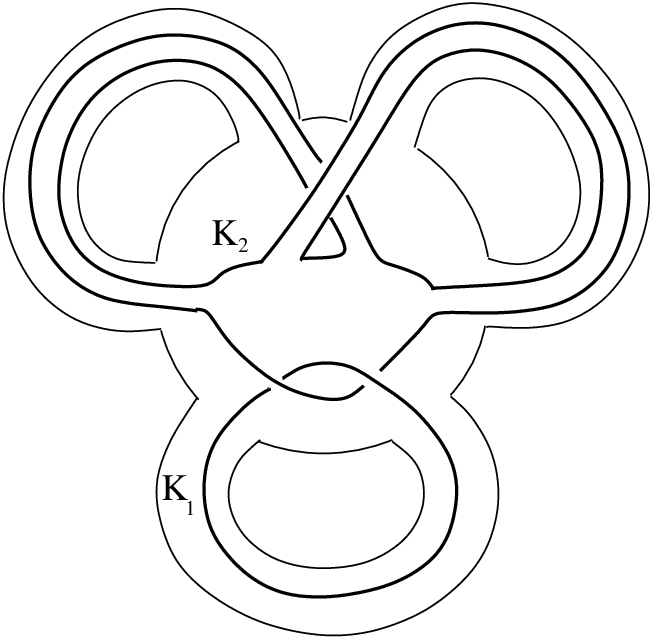
We then have $M_{G}=V_{L\cup K}$ . The linking matrix of $L\cup K$ , when $K$ is appropriately oriented, looks like:

B_{L\cup K}=\left(\begin{array}[]{ccc|cc}&&&x_{1}&0\\ &B_{L}&&\vdots&\vdots\\ &&&x_{l}&0\\ \hline\cr x_{1}&\cdots&x_{l}&x&1\\ 0&\cdots&0&1&0\end{array}\right).

Writing the characteristic condition (11), we find that each characteristic solution of $B_{L\cup K}$ is of the form:

(14)

T_{G}(s):=\left(s_{1},\dots,s_{l},0,x+\sum_{i=1}^{l}x_{i}s_{i}\right)\in(\mathbf{Z}_{2})^{l+2},

where $s=(s_{1},\dots,s_{l})$ must be characteristic for $L$ . Equation (14) then defines a combinatorial bijection: {diagram}

Lemma 7.

With the above notations, the map $T_{G}$ is a combinatorial version of the map $\Theta_{G}$ in terms of characteristic solutions for surgery presentations on $\mathbf{S}^{3}$ . More precisely, the following diagram is commutative: {diagram}

Proof.

This follows from the definitions and from Lemma 6: note that $K_{2}$ is nul-homologous in $H$ , and that here $H_{K}$ is merely a handlebody. ∎

Definition 11.

Let $M=V_{L}$ be a surgery presentation of a $3$ -manifold $M$ on $\mathbf{S}^{3}$ , and let $G$ be a $Y$ -graph in $M$ . Then, $G$ is said to be simple (with respect to this surgery presentation), if $G$ can be isotoped in $M$ so that, in $\mathbf{S}^{3}$ , its leaves bound disjoint discs, each intersecting $L$ in exactly one point.

Corollary 2.

For a $Y^{s}$ -surgery along a simple $Y$ -graph, the spin-diffeomorphism of Figure 8 holds.

Proof.

Replace in the lhs of Figure 8, this simple $Y$ -graph by the 2-component link of Figure 7 such that $K_{1}$ links the $i^{e}$ component of $L$ and use equation (14) to obtain the intermediate link of Figure 9.

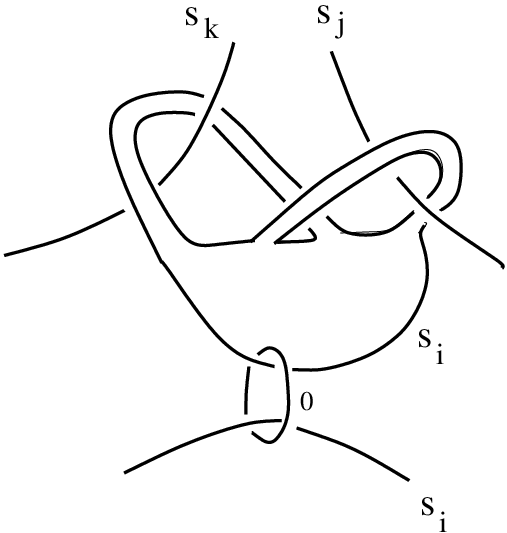
Perform then some spin Kirby moves to obtain the rhs of Figure 8. ∎

Example 3.

As a consequence of Corollary 2, the Lie spin structure of the $3$ -torus is $Y^{s}$ -equivalent to the seven other ones.

Proof.

The two spin structures of $\mathbf{S}^{1}\times\mathbf{S}^{2}$ are equivalent, so are the eight ones of $\sharp^{3}\mathbf{S}^{1}\times\mathbf{S}^{2}$ . Furthermore, $\sharp^{3}\mathbf{S}^{1}\times\mathbf{S}^{2}$ can be obtained from $\mathbf{S}^{3}$ by surgery along a trivial $0$ -framed three-component link. Surgery on the $0$ -framed Borromean rings gives rise to the $3$ -torus $\mathbf{S}^{1}\times\mathbf{S}^{1}\times\mathbf{S}^{1}$ , and this link can be obtained from the trivial link by a simple $Y$ -surgery. ∎

3. Quadratic forms on finite Abelian groups

3.1. Linking pairings, quadratic forms on finite Abelian groups and their presentations.

We recall here standard algebraic constructions: notations are that of Deloup in [De1], where a brief review of the subject can be found.

Definition 12.

A linking pairing on a finite Abelian group $G$ is a nondegenerate symmetric bilinear map $b:G\times G\rTo\mathbf{Q}/\mathbf{Z}$ .
A quadratic form on $G$ is a map $q:G\rTo\mathbf{Q}/\mathbf{Z}$ such that the map $b_{q}:G\times G\rTo\mathbf{Q}/\mathbf{Z}$ defined by $b_{q}(x,y)=q(x+y)-q(x)-q(y)$ is bilinear, and such that $q$ satisfies: $\forall x\in G,\ q(-x)=q(x)$ . $q$ is said to be nondegenerate when the associated bilinear form $b_{q}$ is a linking pairing.

Let now $(F,f)$ be a symmetric bilinear form on a free finitely generated Abelian group $F$ . We denote by $ad_{f}:F\rTo Hom(F,\mathbf{Z})$ the adjoint map, and by $a_{f}:F\otimes\mathbf{Q}\rTo Hom(F,\mathbf{Q})$ its rational extension. Form:

K_{f}:=\frac{Hom(F,\mathbf{Z})\cap Im(a_{f})}{Im(ad_{f})}.

Note that $K_{f}=T\left(Coker(ad_{f})\right)$ , the torsion subgroup of $Coker(ad_{f})$ . We now define a linking pairing:

K_{f}\times K_{f}\rTo^{L_{f}}\mathbf{Q}/\mathbf{Z}

by the formula:

(15)

L_{f}(\bar{x},\bar{y})=x_{\mathbf{Q}}(\tilde{y})\hskip 10.00002ptmod\hskip 10.00002pt1,

where $x,y\in Hom(F,\mathbf{Z})\cap Im(a_{f})$ , $\tilde{y}\in F\otimes\mathbf{Q}$ is such that $a_{f}(\tilde{y})=y$ , and $x_{\mathbf{Q}}\in Hom(F\otimes\mathbf{Q},\mathbf{Q})$ is the rational extension of $x$ . $(F,f)$ is said to be a presentation of the linking pairing $(K_{f},L_{f})$ .

Suppose now that the form $(F,f)$ comes equipped with a Wu class, that is an element $w\in F$ such that $\forall x\in F,f(w,x)=f(x,x)\hskip 10.00002ptmod\hskip 10.00002pt2$ . We can then define a quadratic form over $L_{f}$ , denoted by:

K_{f}\rTo^{\phi_{f,w}}\mathbf{Q}/\mathbf{Z}

and defined by:

(16)

\phi_{f,w}(\bar{x})=\frac{1}{2}\left(x_{\mathbf{Q}}(\tilde{x})-x(w)\right)\hskip 10.00002ptmod\hskip 10.00002pt1.

$\phi_{f,w}$ is determined by the modulo $2F$ class of $w$ . The triple $(F,f,w)$ is said to be a presentation of the quadratic form $\left(K_{f},\phi_{f,w}\right)$ .
Any linking pairing and any nondegenerate quadratic form admit such presentations with $f$ nondegenerate (see [Wa1, Theorem (6)]).

Given an arbitrary quadratic form on a finite Abelian group $(G,q)$ , we can calculate its Gauss sum:

\gamma(G,q)=\frac{1}{\sqrt{|ker(b_{q})|\cdot|G|}}\cdot\sum_{\begin{subarray}{c}x\in G\end{subarray}}e^{2i\pi q(x)}\in\mathbf{C}.

This complex number is a $8^{\textrm{e}}$ -root of unity or is $0$ (only if $q$ is degenerate).
We then define the corresponding Gauss-Brown invariant $B(G,q)\in\overline{\mathbf{Z}_{8}}=\mathbf{Z}_{8}\cup\{\infty\}$ by the formula:

(17)

\gamma(G,q)=e^{\frac{2i\pi}{8}\cdot B(G,q)}\in\mathbf{C},

using the convention $e^{2i\pi\cdot\infty}=0$ .
If $(G,q)$ admits a triple $(F,f,w)$ as a presentation, a useful formula of Van der Blij states that²² 2 A sketch of proof of this formula can be found in [VdB], in case when $f$ is nondegenerate.
Milnor and Husemoller have included a detailed proof in [MH, Appendix 4], for $f$ nondegenerate and $w=0$ . The general case can be reduced to this special case.:

(18)

B(K_{f},\phi_{f,w})=sgn(f)-f(w,w)\hskip 10.00002ptmod\hskip 10.00002pt8.

For $(G,b)$ a linking pairing, denote by $Quad(G,b)$ the set of quadratic forms with $b$ as associated linking pairing, and denote by $T_{2}(G)$ the subgroup of elements of $G$ of order at most $2$ . Using the nondegenerativity of $b$ , we easily obtain:

Lemma 8.

The set $Quad(G,b)$ is an affine space over $T_{2}(G)$ , with action defined by:

\forall x\in T_{2}(G),\ \forall q\in Quad(G,b),\ x\cdot q:=q+b(x,-).

The following lemma says how the Gauss-Brown invariant behaves under this action.

Lemma 9.

Let $q\in Quad(G,b)$ and let $x\in T_{2}(G)$ . Then,

\gamma(G,x\cdot q)=e^{-2i\pi q(x)}\cdot\gamma(G,q).

Proof.

Since $(x\cdot q)(y)=q(y)+b(x,y)=q(x+y)-q(x)$ , we have:

\begin{array}[]{rcl}\sqrt{|G|}\cdot\gamma(G,x\cdot q)&=&\sum_{y\in G}e^{2i\pi(x\cdot q)(y)}\\ &=&e^{-2i\pi q(x)}\cdot\sum_{y\in G}e^{2i\pi q(x+y)}\\ &=&e^{-2i\pi q(x)}\cdot\sqrt{|G|}\cdot\gamma(G,q)\end{array}

∎

3.2. Isomorphism classes of nondegenerate quadratic forms

We now want to prove the following result:

Theorem 2.

Let $(G,q)$ and $(G^{\prime},q^{\prime})$ be two nondegenerate quadratic forms on finite Abelian groups. We denote by $b$ and $b^{\prime}$ the linking pairings going respectively with them. The following two assertions are equivalent:

(1)

$(G,q)\simeq(G^{\prime},q^{\prime})$ ,
(2)

$(G,b)\simeq(G^{\prime},b^{\prime})$ and $B(q)=B(q^{\prime})\in\mathbf{Z}_{8}$ ,

where $B(-)$ denotes the Gauss-Brown invariant of quadratic forms.

Let $(G,q)$ (respectively $(G^{\prime},q^{\prime})$ ) be a nondegenerate quadratic form over the linking pairing $(G,b)$ (respectively $(G^{\prime},b^{\prime})$ ). Recall that the relation between $b$ and $q$ is:

(19)

b(x,y)=q(x+y)-q(x)-q(y).

From this formula and the definition of $B(-)$ , “ $1\Rightarrow 2$ ” of Theorem 2 is obvious.

Suppose momentarily that $G$ is a $p$ -group, with $p$ an odd prime. Then, equation $2q(x)=b(x,x)$ makes $b$ determine $q$ , for if $q^{\prime\prime}$ is another quadratic form over $b$ , then $(q-q^{\prime\prime})$ is an order at most $2$ element of $Hom\left(G,\mathbf{Q}/\mathbf{Z}\right)\simeq G$ , and so vanishes. So, if $G$ and $G^{\prime}$ are both $p$ -groups, then $b\simeq b^{\prime}$ implies $q\simeq q^{\prime}$ .

Come back now to the general case and suppose that condition 2 is satisfied. $(G,b)$ splits along its $p$ -primary components $G_{p}$ :

(G,b)=\bigoplus_{p,\textrm{ prime }}\left(G_{p},b|_{G_{p}\times G_{p}}\right),

and, according to formula (19), the same holds for $q$ . The given isomorphism between $(G,b)$ and $(G^{\prime},b^{\prime})$ , induces then for each prime $p$ an isomorphism between $\left(G_{p},b|_{G_{p}\times G_{p}}\right)$ and $\left(G^{\prime}_{p},b^{\prime}|_{G^{\prime}_{p}\times G^{\prime}_{p}}\right)$ . From the above lines, we deduce that, for $p$ odd, $\left(G_{p},q|_{G_{p}}\right)$ and $\left(G^{\prime}_{p},q^{\prime}|_{G^{\prime}_{p}}\right)$ are isomorphic.
In particular, $B\left(q|_{G_{p}}\right)=B\left(q^{\prime}|_{G^{\prime}_{p}}\right)$ for $p$ odd, and so, by additivity of the Gauss-Brown invariant, this is also true for $p=2$ . Consequently, it is enough to prove Theorem 2 when $G$ and $G^{\prime}$ are $2$ -groups.

In the sequel, we recall a construction due to Wall (see [Wa1, §6]), establishing a one to one correspondence (up to isomorphism) between nondegenerate quadratic forms on $2$ -groups and linking pairings on $2$ -groups without direct summand of order two. Next, we give a brief review of Kawauchi and Kojima classification of linking pairings on $2$ -groups. We will finally end the proof of Theorem 2.

Wall construction

A linking pairing $(G^{\prime},b^{\prime})$ will be said here to be special if $G^{\prime}$ is a finite $2$ -group without direct summand of order two.
Let give us a special linking pairing $(G^{\prime},b^{\prime})$ . Set $G:=G^{\prime}/T_{2}(G^{\prime})$ where $T_{2}(G^{\prime})$ is the subgroup of elements of order at most $2$ , and denote by $\pi$ the canonical projection $G^{\prime}\rTo G$ . Note that $G$ can be any $2$ -group. Define now $q:G\rTo\mathbf{Q}/\mathbf{Z}$ by:

\forall x=\pi(x^{\prime})\in G,\hskip 10.00002ptq(x)=b^{\prime}(x^{\prime},x^{\prime}).

The quantity $q(x)$ is well-defined because of the special feature of the group $G^{\prime}$ .
Then, $q$ is easily seen to be quadratic and nondegenerate, with associated linking pairing $b:G\times G\rTo\mathbf{Q}/\mathbf{Z}$ defined by:

(20)

\forall x=\pi(x^{\prime}),\ \forall y=\pi(y^{\prime})\in G,\ b(x,y)=2\cdot b^{\prime}(x^{\prime},y^{\prime}).

Let us denote by $\Psi$ the construction $(G^{\prime},b^{\prime})\rMapsto(G,q)$ . Wall showed this to be surjective onto the set of nondegenerate quadratic forms on $2$ -groups. He also proved that if $(G^{\prime},b^{\prime}_{1})$ and $(G^{\prime},b^{\prime}_{2})$ give rise to the same $(G,q)$ by $\Psi$ , then they have to be isomorphic (see [Wa1, Theorem 5]).

As a consequence, the classification, up to isomorphism, of nondegenerate quadratic forms on $2$ -groups is reduced to that of special linking pairings.

Kawauchi-Kojima classification of linking pairings on 2-groups

Let $(G,b)$ be a linking pairing on a finite $2$ -group. Find a cyclic decomposition of $G$ :

G\simeq\bigoplus_{k\geq 1}\left(\mathbf{Z}_{2^{k}}\right)^{r_{k}}.

The natural numbers $r_{k}=r_{k}(b)$ are group invariants of $G$ . The very next construction is due to Wall (see [Wa1, §5]).

Denote by $\overline{G}_{k}$ the subgroup of $G$ of elements of order at most $2^{i}$ for $i\leq k$ , and set:

\tilde{G}_{k}=\frac{\overline{G}_{k}}{\overline{G}_{k-1}+2\cdot\overline{G}_{k+1}}.

The group $\tilde{G}_{k}$ is clearly a $\mathbf{Z}_{2}$ -vector space of rank $r_{k}$ . Let also $\tilde{b}_{k}:\tilde{G}_{k}\times\tilde{G}_{k}\rTo\mathbf{Q}/\mathbf{Z}$ be defined by:

\forall x,y\in\overline{G}_{k},\hskip 10.00002pt\tilde{b}_{k}(\tilde{x},\tilde{y})=2^{k-1}\cdot b(x,y).

The form $\tilde{b}_{k}$ was shown by Wall to be nondegenerate (see [Wa1, Lemma 8]).

Consider now the map $\tilde{G}_{k}\rTo\mathbf{Q}/\mathbf{Z}$ sending $\tilde{x}$ to $\tilde{b}_{k}(\tilde{x},\tilde{x})$ . It is additive, and so we can define an element $\tilde{c}_{k}=\tilde{c}_{k}(b)$ in $\tilde{G}_{k}$ by the equation:

(21)

\forall\tilde{x}\in\tilde{G}_{k},\hskip 10.00002pt\tilde{b}_{k}(\tilde{x},\tilde{c}_{k})=\tilde{b}_{k}(\tilde{x},\tilde{x}).

When $\tilde{c}_{k}=0$ , the following map can be defined:

\left\{\begin{array}[]{rrcl}\frac{G}{\overline{G}_{k}}&\rTo^{q_{k}}&\frac{\mathbf{Q}}{\mathbf{Z}}\\ \bar{x}&\rMapsto&2^{k-1}\cdot b(x,x).\end{array}\right.

The form $q_{k}=q_{k}(b)$ can be verified to be quadratic and nondegenerate. In particular, its Gauss-Brown invariant $B(q_{k})$ is not equal to $\infty$ .
Kawauchi and Kojima defined $\sigma_{k}=\sigma_{k}(b)\in\overline{\mathbf{Z}_{8}}$ by:

\sigma_{k}=\left\{\begin{array}[]{ll}B(q_{k})&\textrm{if }\tilde{c}_{k}=0,\\ \infty&\textrm{otherwise,}\end{array}\right.

and showed the following theorem (see [KK, Theorem 4.1]).

Theorem 3 (Kawauchi-Kojima).

If $(G,b)$ is a linking pairing on a finite $2$ -group, its isomorphism class is determined by the invariant family $\left(r_{k}(b),\sigma_{k}(b)\right)_{k\geq 1}$ .

End of proof of Theorem 2.

Let $(G,q)$ be a quadratic form on a finite $2$ -group $G$ , going with a linking pairing $b$ . Let also $(G^{\prime},b^{\prime})$ be a special linking pairing, giving rise to $(G,q)$ by Wall construction $\Psi$ .

We want to compare the invariants $r_{k}$ and $\sigma_{k}$ of $b$ and $b^{\prime}$ , in order to quantify how much $(G,b)$ determines $(G^{\prime},b^{\prime})$ , and so $(G,q)$ , up to isomorphism.
Recall that $G=G^{\prime}/\overline{G^{\prime}}_{1}$ . Denote by $\pi:G^{\prime}\rTo G$ the canonical projection. The map $\pi$ induces a morphism from $\overline{G^{\prime}}_{k+1}$ onto $\overline{G}_{k}$ with kernel $\overline{G^{\prime}}_{1}$ . So, $\pi$ induces a natural isomorphism: {diagram} In particular, the $\mathbf{Z}_{2}$ -vector spaces $\tilde{G^{\prime}}_{k+1}$ and $\tilde{G}_{k}$ have the same rank. So,

(22)

\forall k\geq 1,\hskip 10.00002ptr_{k+1}(G^{\prime})=r_{k}(G).

Besides, since $G^{\prime}$ is special, we have:

(23)

r_{1}(G^{\prime})=0.

The isomorphism $\tilde{\pi}_{k}$ makes $\tilde{b^{\prime}}_{k+1}$ and $\tilde{b}_{k}$ commute because of equation (20). As a consequence, $\tilde{\pi}_{k}$ sends $\tilde{c}_{k+1}(b^{\prime})$ to $\tilde{c}_{k}(b)$ . Furthermore, when these (simultaneously) vanish, the natural isomorphism between $G^{\prime}/\overline{G^{\prime}}_{k+1}$ and $G/\overline{G}_{k}$ induced by $\pi$ , make $q_{k+1}(b^{\prime})$ and $q_{k}(b)$ commute (because of equation (20)). As a consequence, these two quadratic forms will have the same Gauss-Brown invariant. So, to sum up,

(24)

\forall k\geq 1,\hskip 10.00002pt\sigma_{k+1}(b^{\prime})=\sigma_{k}(b)\in\overline{\mathbf{Z}_{8}}.

Since $\tilde{G^{\prime}}_{1}=0$ , $\tilde{c}_{1}(b^{\prime})$ vanishes. It remains to be noticed that $q_{1}(b^{\prime})$ is nothing but $q$ . Thus,

(25)

\sigma_{1}(b^{\prime})=B(q).

Now, from equations (22), (23), (24), (25) and Kawauchi-Kojima theorem, we see that $(G,b)$ together with $B(q)$ determine $(G,q)$ up to isomorphism. What has been remaining to be proved for Theorem 2, then follows. ∎

We now give a result of Durfee (see [Du, Corollary 3.9]) as a corollary of Theorem 2.

Corollary 3.

Let $b:G\times G\rTo\mathbf{Q}/\mathbf{Z}$ be a linking pairing on a finite Abelian group $G$ without cyclic direct summand of order $2$ or $4$ . Then, $\forall q,q^{\prime}\in Quad(G,b),\ q\simeq q^{\prime}$ .

Proof.

Take some quadratic forms $q$ and $q^{\prime}$ over $b$ , and let $x\in T_{2}(G)$ be such that $q^{\prime}=x\cdot q$ (see Lemma 8). By the hypothesis on $G$ , there exits some $x_{0}\in G$ such that $x=4x_{0}$ , and so, by homogeneity of $q$ , we have:

q(x)=q(4x_{0})=4^{2}q(x_{0}).

But since $x_{0}$ is then of order at most $8$ , $q(x_{0})$ has to be of order at most $2\cdot 8=16$ (see [De2, Lemma 1.12]). It follows that $q(x)=0$ and so, by Lemma 9, we obtain that $B(G,q)=B(G,q^{\prime})$ . Theorem 2 allows us to conclude. ∎

4. The quadratic form $\phi_{M,\sigma}$

In this section, when not specified, integer coefficients are assumed.

4.1. Turaev $4$ -dimensional definition of $\phi_{M,\sigma}$

Let $M$ be a connected closed oriented $3$ -manifold, and let $\psi:V_{L}\rTo M$ be a surgery presentation on $\mathbf{S}^{3}$ given by an ordered oriented framed link $L$ (see the beginning of §2.6).
We use notations and apply constructions of §3.1 to $F=H_{2}(W_{L})$ , taking for $f$ the intersection form of $W_{L}$ . Recall that the matrix of $f$ relative to the preferred basis of $F$ is $B_{L}$ , the linking matrix of $L$ .
The composite: {diagram} is equal to $i_{*}:H_{2}(W_{L})\rTo H_{2}(W_{L},\partial W_{L})$ , induced by inclusion. Since $Coker(i_{*})=H_{1}(V_{L})$ , we obtain the following isomorphism $r$ : {diagram} In fact, it is well-known that the above $(F,-f)$ is via $r$ a presentation of the torsion linking form $\big(TH_{1}(M),\lambda_{M}\big)$ of $M$ , the definition of which we now recall:

Let $x,x^{\prime}\in TH_{1}(M)$ be respectively realized by oriented disjoint knots $K,K^{\prime}$ in $M$ . Let $c^{\prime}\in\mathbf{N}$ be such that $c^{\prime}\cdot x^{\prime}=0$ . Pick a $c^{\prime}$ -times connected sum of $K^{\prime}$ . We obtain a null-homologous knot in $M$ for which we can thus find a Seifert surface $S^{\prime}$ in general position with $K$ . Then:

$\lambda_{M}(x,x^{\prime})=\frac{1}{c^{\prime}}K\bullet S^{\prime}\in\mathbf{Q}/\mathbf{Z},$

where $\bullet$ is the intersection form of $M$ .

Now to each $\sigma\in Spin(M)$ is associated a characteristic solution of $-B_{L}$ or, alternatively, a Wu class (modulo $2F$ ) of $-f$ , denoted by $w_{\sigma}$ . Then, Turaev defined:

Definition 13.

The quadratic form of the spin $3$ -manifold $(M,\sigma)$ : {diagram} is defined to be $\phi_{-f,w_{\sigma}}\circ r^{-1}$ .

We still have to verify that $\phi_{M,\sigma}$ does not depend on the choice of the surgery presentation.
Let $\psi^{\prime}:V_{L^{\prime}}\rTo M$ be another one. Let $s\in(\mathbf{Z}_{2})^{l}$ (resp. $s^{\prime}$ ) be the characteristic solution of $B_{L}$ (resp. $B_{L^{\prime}}$ ) corresponding to the spin structure $\psi^{*}(\sigma)$ of $V_{L}$ (resp. $(\psi^{\prime})^{*}(\sigma)$ of $V_{L^{\prime}}$ ).
According to the refined Kirby theorem (see [Bl]), there exists a sequence of spin Kirby moves from $(L,s)$ to $(L^{\prime},s^{\prime})$ , inducing a spin-diffeomorphism from $\left(V_{L},\psi^{*}(\sigma)\right)$ to $\left(V_{L^{\prime}},(\psi^{\prime})^{*}(\sigma)\right)$ isotopic to $(\psi^{\prime})^{-1}\circ\psi$ . These Kirby moves induce a path $(F,f,w_{\sigma})\leadsto(F^{\prime},f^{\prime},w^{\prime}_{\sigma})$ whose elementary steps are:

\left\{\begin{array}[]{ll}(F,f,w)\rMapsto\left(F,{}^{t}SfS,S^{-1}(w)\right)&\textrm{with }S\in Aut(F),\\ (F,f,w)\rMapsto\left(F\oplus\mathbf{Z},f\oplus(\pm 1),w\oplus(1)\right).&\end{array}\right.

As a consequence, this path induces an isomorphism $t$ from $\left(K_{f},\phi_{f,w_{\sigma}}\right)$ to $\left(K_{f^{\prime}},\phi_{f^{\prime},w^{\prime}_{\sigma}}\right)$ making the following diagram commutative: {diagram} The well-definition of $\phi_{M,\sigma}$ then follows.

4.2. An intrinsic definition for $\phi_{M,\sigma}$

Let $(M,\sigma)$ be a closed spin $3$ -manifold and let $K$ be a smooth oriented knot in $M$ .
Each parallel $l$ of $K$ defines a trivialization of the normal bundle of $K$ in $M$ , and so allows us to restrict $\sigma$ to a spin structure on $K\cong\mathbf{S}^{1}$ . We define:

\sigma(K,l)=\left\{\begin{array}[]{ll}0&\textrm{ if the induced spin structure on }\mathbf{S}^{1}\textrm{ is the ``bounding'' one,}\\ 1&\textrm{ otherwise.}\end{array}\right.

$\sigma(K,l)$ is a $\mathbf{Z}_{2}$ -valued invariant of framed knots in $M$ .

Lemma 10.

Let $(M,\sigma)$ be a closed spin $3$ -manifold. Then, for each oriented smooth knot $K$ in $M$ with $l$ as a parallel and meridian $\mu$ ,

\sigma(K,l+\mu)=\sigma(K,l)+1\in\mathbf{Z}_{2}.

Proof.

Let $S$ denote the boundary of a regular neighbourhood of $K$ in $M$ . The normal bundle of $S$ in $M$ is naturally trivialized, so $S$ inherits from $(M,\sigma)$ a spin structure. Let $q$ be the quadratic form associated to the spin smooth surface $\left(S,\sigma|_{S}\right)$ as defined by Johnson in [Jo]. The following identity then holds for each parallel $l$ :

\sigma(K,l)=q\left([l]\right),

when $l$ is thought of as a curve on $S$ . Since $q$ is quadratic with respect to the modulo $2$ intersection form $\bullet$ on $S$ , we have:

\begin{array}[]{rcl}\sigma(K,l+\mu)&=&q\left([l]+[\mu]\right)\\ &=&q\left([l]\right)+q\left([\mu]\right)+[l]\bullet[\mu]\\ &=&q\left([l]\right)+1\\ &=&\sigma(K,l)+1.\end{array}

∎

We now recall the definition of the framing number $Fr(K,l)\in\mathbf{Q}$ of a rationally nulhomologous oriented framed knot $(K,l)$ in a closed oriented $3$ -manifold $M$ :

Choose $c\in\mathbf{N}^{*}$ such that $c\cdot[K]=0\in H_{1}(M)$ . Pick a $c$ -times connected sum of $K$ . We obtain a null-homologous knot in $M$ for which we can thus pick a Seifert surface $S$ in general position with the knot $l$ . Then:

$Fr(K,l)=\frac{1}{c}\cdot l\bullet S\in\mathbf{Q}.$

Lemma 11.

Let $(M,\sigma)$ be a closed spin $3$ -manifold and $x\in TH_{1}(M)$ . Choose a smooth oriented knot $K$ in $M$ representative for $x$ , and pick a parallel $l$ for $K$ satisfying $\sigma(K,l)=0\in\mathbf{Z}_{2}$ . Then,

(26)

\phi_{M,\sigma}(x)=\frac{1}{2}\cdot Fr(K,l)\in\frac{\mathbf{Q}}{\mathbf{Z}}.

Note that, according to Lemma 10, the rhs of (26) is an invariant of the oriented knot $K$ (it does not depend on the choice of $l$ satisfying the above condition). This lemma claims that it only depends on the homology class $x$ of $K$ , and gives a $3$ -dimensional definition for the quadratic form $\phi_{M,\sigma}$ .

Remark 4.

From this lemma, we can see that $\phi_{M,\sigma}$ coincides with the quadratic form defined by Lannes and Latour in [LL] when specialized to our case (see also [MS]).

Proof of Lemma 11.

Consider the $4$ -manifold $W_{1}$ obtained from $M\times[0,1]$ by attaching a $2$ -handle to $M\times 1$ along $(K,l)$ . Identify $M$ with $M\times 0$ . Since $\sigma(K,l)=0$ , $\sigma$ extends in a unique way to a spin structure $\sigma_{1}$ of $W_{1}$ .
$(W_{1},\sigma_{1})$ is then a spin cobordism between $(M,\sigma)$ and $(-M^{\prime},-\sigma^{\prime})$ , where $M^{\prime}$ is the closed oriented $3$ -manifold obtained from $M$ by the corresponding surgery, and where $-\sigma^{\prime}$ is the restriction of $\sigma_{1}$ to $-M^{\prime}$ .
Note also that the core of the $2$ -handle is a $2$ -disc $D$ in $W_{1}$ with boundary $K$ in $M$ , and whose normal bundle can be trivialized in accordance with the trivialization of the normal bundle of $K$ in $M$ given by $l$ . The framed knot $(K,l)$ will briefly be said to have property $(\mathcal{D})$ in $W_{1}$ .
According to Kaplan Theorem (see [Ka]), the spin $3$ -manifold $(M^{\prime},\sigma^{\prime})$ admits an even surgery presentation in $\mathbf{S}^{3}$ (i.e. the linking matrix is even and its characteristic solution corresponding to $\sigma^{\prime}$ is the trivial one). Denote by $W_{2}$ the trace of the surgery and by $\sigma_{2}$ the unique extension of $\sigma^{\prime}$ to the whole of $W_{2}$ .
By glueing $(W_{1},\sigma_{1})$ to $(W_{2},\sigma_{2})$ along $(M^{\prime},\sigma^{\prime})$ , we obtain a spin $4$ -manifold $(W,\sigma)$ with boundary $(M,\sigma)$ . The $2$ -handle from $M$ to $M^{\prime}$ can be reversed. After a rearrangement, the $4$ -manifold $W$ appears as $\mathbf{B}^{4}$ to which have been simultaneously attached some $2$ -handles (one more than $W_{2}$ ), with boundary $M$ , and to which $\sigma$ can be extended. So, $W$ is the trace of an even surgery presentation.

As a summary, we have found so for an even surgery presentation $(L,0)$ for $(M,\sigma)$ such that $(K,l)$ has property ( $\mathcal{D}$ ) in $W_{L}$ .

Let us work with this surgery presentation of $(M,\sigma)$ . Notations of §4.1 will be used: $F=H_{2}(W_{L})$ , $f$ stands for the intersection form of $W_{L}$ and so on.
Let the $2$ -disc $D$ give an element of $H_{2}(W_{L},\partial W_{L})$ . The latter is identified with an element $d$ of $Hom(F,\mathbf{Z})$ . Recall from the definition of $\phi_{M,\sigma}$ that, in this even case,

(27)

\phi_{M,\sigma}(x)=-\frac{1}{2}d_{\mathbf{Q}}(\tilde{d}),

where $d_{\mathbf{Q}}$ is the rational extension of $d$ and where $\tilde{d}\in F\otimes\mathbf{Q}$ is such that $a_{f}(\tilde{d})=d$ .
Let $c\in\mathbf{N}$ such that $c\cdot x=0\in H_{1}(M)$ . Then, there exists $y\in F$ such that $ad_{f}(y)=c\cdot d$ . So $\frac{1}{c}\cdot y\in F\otimes\mathbf{Q}$ works as a $\tilde{d}$ . Equation (27) can be rewritten as:

(28)

\phi_{M,\sigma}(x)=-\frac{1}{2c^{2}}f(y,y).

When $y$ is seen as belonging to $H_{2}(W_{L})$ , the integer $f(y,y)$ is equal to $Y\bullet Y^{\prime}$ , where $Y$ and $Y^{\prime}$ are $2$ -cycles representatives for $y$ in transverse position in $W_{L}$ . By means of a “collar” trick appearing in [De2], we will be able to give examples of such $Y$ and $Y^{\prime}$ .
We add a collar $M\times[0,1]$ to $W_{L}$ such that $M\times 0$ is identified with $M$ . Let $S$ be a Seifert surface for $c\cdot K$ in $M$ in transverse position with $l$ , and $S^{\prime}$ be a Seifert surface for $(c\cdot l)\times 1$ in $M\times 1$ . Because of the property $(\mathcal{D})$ , $D$ can be pushed off to a disc $D^{\prime}$ in such a way that $\partial D^{\prime}=l$ and $D\cap D^{\prime}=\varnothing$ . Figure 10 is a good summary.

We define $Y=c.D-S$ and $Y^{\prime}=\left(c.D^{\prime}+(c.l)\times[0,1]\right)-S^{\prime}$ . Then:

(29)

f(y,y)=Y\bullet Y^{\prime}=(-S)\bullet(c.D^{\prime})=-c\cdot S\bullet l.

The last $\bullet$ in (29) is intersection in $M$ . The lemma follows from (29), (28) and the definition of a framing number. ∎

4.3. Properties of $\phi_{M,\sigma}$

The algebraic results of §3 have a topological meaning. First, it has been shown by Turaev in [Tu, Theorem V]:

Lemma 12 (Turaev).

For each $\sigma\in Spin(M)$ , $B(\phi_{M,\sigma})=-R_{M}(\sigma)\hskip 10.00002ptmod\hskip 10.00002pt8$ ,
where $R_{M}$ is the Rochlin function of the $3$ -manifold $M$ .

Proof.

Find an even surgery presentation of the spin $3$ -manifold $(M,\sigma)$ . So we are led to apply formula (18) with $w=0$ . ∎

So, in view of Lemma 12, the topological translations of Theorem 2 and its Corollary 3 are respectively:

Proposition 2.

Let $(M,\sigma)$ and $(M^{\prime},\sigma^{\prime})$ be connected closed spin $3$ -manifolds.
The following two assertions are equivalent:

(1)

their quadratic forms $\phi_{M,\sigma}$ and $\phi_{M^{\prime},\sigma^{\prime}}$ are isomorphic,
(2)

their linking forms $\lambda_{M}$ and $\lambda_{M^{\prime}}$ are isomorphic, and $R_{M}(\sigma)=R_{M^{\prime}}(\sigma^{\prime})$ modulo $8$ .

Corollary 4.

Let $M$ be a connected closed oriented $3$ -manifold, such that $H_{1}(M)$ does not admit $\mathbf{Z}_{2}$ nor $\mathbf{Z}_{4}$ as a direct summand. Then, all of its quadratic forms are isomorphic one to another.

5. Proof of refined Matveev theorem

Part of the work has already been done in previous sections. First, “ $1\Longrightarrow 3$ ” follows from Corollary 1 and from the easy part of (unspun) Matveev theorem: a $Y$ -surgery preserves homology and torsion linking forms. This can be verified seeing $Y$ -surgery as a $\mathcal{V}_{h}$ -surgery (where $h$ is the Borromean diffeomorphism of Remark 1), using a Mayer-Vietoris argument and the fact that $h$ belongs to the Torelli group. Second, “ $3\Longrightarrow 2$ ” follows from Proposition 2. What remains to be proved is then “ $2\Longrightarrow 1$ ”.

We start by recalling an algebraic result of Durfee (see [Du]) about even symmetric bilinear forms on finitely generated free Abelian groups.
Let $(\mathbf{Z}^{2},h)$ and $(\mathbf{Z}^{8},\gamma_{8})$ be the unimodular even forms whose matrices are respectively:

H=\left(\begin{array}[]{cc}0&1\\ 1&0\end{array}\right)\hskip 20.00003pt\textrm{and}\hskip 20.00003pt\Gamma_{8}=\left(\begin{array}[]{cccccccc}2&1&&&&&&\\ 1&2&1&&&&&\\ &1&2&1&&&&\\ &&1&2&1&&&\\ &&&1&2&1&0&1\\ &&&&1&2&1&0\\ &&&&0&1&2&0\\ &&&&1&0&0&2\end{array}\right).

Definition 14.

Let $(F_{1},f_{1})$ and $(F_{2},f_{2})$ be two symmetric even bilinear forms on finitely generated free Abelian groups. They are said to be stably equivalent if they become isomorphic after some stabilizations with unimodular symmetric even bilinear forms.

Note that a unimodular even form becomes indefinite after taking direct sum with $h$ . Recall that every even unimodular indefinite form splits as a direct sum of $h$ and $\gamma_{8}$ (see for example [Ki, p.26]). Thus, in Definition 14, $h$ and $\gamma_{8}$ suffice as unimodular even forms to stabilize.

For $(F,f)$ an even symmetric bilinear form on a finitely generated free Abelian group, we will shortly denote by $\phi_{f}$ the quadratic form $\phi_{f,0}$ corresponding to the zero Wu class.

Proposition 3 (Durfee).

Let $(F_{1},f_{1})$ and $(F_{2},f_{2})$ be two symmetric even bilinear forms on finitely generated free Abelian groups. Then, the following two assertions are equivalent:

(1)

$(F_{1},f_{1})$ and $(F_{2},f_{2})$ are stably equivalent,
(2)

$Ker\left(ad_{f_{1}}\right)\simeq Ker\left(ad_{f_{2}}\right)$ and $\phi_{f_{1}}\simeq\phi_{f_{2}}$ .

Proof.

Implication “1 $\Rightarrow$ 2” is obvious since $\gamma_{8}$ and $h$ are both unimodular.
Now suppose that condition 2 is satisfied. For each $i\in\{1,2\}$ , there exists a nondegenerate symmetric bilinear form $\left(\tilde{F}_{i},\tilde{f}_{i}\right)$ such that:

(F_{i},f_{i})\simeq\left(\tilde{F}_{i},\tilde{f}_{i}\right)\oplus(\mathbf{Z}^{r},O_{r})

where $\tilde{F}_{i}=F_{i}/Ker\left(ad_{f_{i}}\right)$ (note that it is free), $r=rk\left(Ker\left(ad_{f_{1}}\right)\right)=rk\left(Ker\left(ad_{f_{2}}\right)\right)$ , and $O_{r}$ is the zero form. The form $\tilde{f}_{i}$ is still even and $\phi_{\tilde{f}_{1}}$ and $\phi_{\tilde{f}_{2}}$ are still isomorphic.
Consequently, without loss of generality, we can assume both $f_{i}$ to be nondegenerate. But this case was treated by Durfee in [Du, Corollary 4.2.(ii)]³³ 3 An easier and direct proof of this result was given by Wall in [Wa2, Corollary 1].. ∎

Let $(M,\sigma)$ and $(M^{\prime},\sigma^{\prime})$ be connected closed spin $3$ -manifolds such that $\beta_{1}(M)=\beta_{1}(M^{\prime})$ and $\phi_{M,\sigma}\simeq\phi_{M^{\prime},\sigma^{\prime}}$ .
Suppose given for them some even surgery presentations $(L,0)$ and $(L^{\prime},0)$ with respective linking matrices $B$ and $B^{\prime}$ . According to Proposition 3, there exists a unimodular integer matrix $P$ satisfying for some stabilizations:

{}^{t}P\cdot(B\oplus H\cdots H\oplus\Gamma_{8}\cdots\Gamma_{8})\cdot P=B^{\prime}\oplus H\cdots H\oplus\Gamma_{8}\cdots\Gamma_{8}.

We have the following geometric realizations of algebraic operations:

(1)

stabilizations by $H$ correspond to connected sums with $\mathbf{S}^{3}$ surgery presented on the zero-framed Hopf link,
(2)

a stabilization by $\Gamma_{8}$ is concrete when thought of as a connected sum with the Poincaré sphere surgery presented on an appropriate height-component link as in [Ki, Figure 5.3, p.15],
(3)

congruence by $P$ can be realized by some spin Kirby moves (handle-slidings and changes of orientation of components of $L$ ).

The Poincaré sphere can also be obtained by surgery along a $(+1)$ -framed trefoil knot ([Ki, Figure 5.3, p.15]), which can be obtained from the $(+1)$ -framed unknot by a simple $Y$ -surgery (see Definition 11). As a consequence, the Poincaré sphere and the sphere $\mathbf{S}^{3}$ , equipped with their unique spin structures, are $Y^{s}$ -equivalent. Since $Y^{s}$ -equivalence is compatible with connected sums, we can assume that $B=B^{\prime}$ .

A theorem of Murakami and Nakanishi ([MN, Theorem 1.1]⁴⁴ 4 In fact, the first reference is Matveev, but the proof in [Ma] is not detailed.) states that two ordered oriented links have identical linking matrices if and only if they are $\Delta$ -equivalent. A $\Delta$ -move is a certain unknotting operation, which is equivalent to surgery along a simple $Y$ -graph.
Finally, from Corollary 2, we see that a simple $Y^{s}$ -surgery between even surgery presentations leaves the trivial characteristic solution fixed. We conclude that $(M,\sigma)$ is $Y^{s}$ -equivalent to $(M^{\prime},\sigma^{\prime})$ , which completes the proof.

6. Applications

According to Theorem 1, two connected closed spin $3$ -manifolds are $Y^{s}$ -equivalent if and only if they are $Y$ -equivalent as plain $3$ -manifolds and their Rochlin invariants are identical modulo $8$ . In other words, while studying the degree $0$ part of Goussarov-Habiro theory, the spin problem can be “factored out”.

Now, given a closed connected oriented $3$ -manifold, one can wonder whether all of its spin structures are $Y^{s}$ -equivalent one to another. This has been verified to be true in the case of $\mathbf{S}^{1}\times\mathbf{S}^{1}\times\mathbf{S}^{1}$ by a direct calculation (Example 3). More generally we have:

Corollary 5.

Let $M$ be a connected oriented closed $3$ -manifold such that $H_{1}(M)$ has no cyclic direct summand of order $2$ or $4$ . Then, all spin structures of $M$ are $Y^{s}$ -equivalent one to another.

Proof.

This follows directly from Theorem 1 and Corollary 4. ∎

On the contrary, we have:

Example 4.

The two spin structures of $\mathbf{RP}^{3}$ are not $Y^{s}$ -equivalent, for the Rochlin function of $\mathbf{RP}^{3}$ takes $1$ and $-1$ as values.

References

[Bl] C. Blanchet, Invariants on three-manifolds with spin-structure, Comment. Math. Helvitici $\mathbf{67}$ (1992), 406–427.
[CM] T.D. Cochran, P. Melvin, Finite type invariants of $3$ -manifolds, Invent. Math. $\mathbf{140}$ (2000), 45–100.
[De1] F. Deloup, Linking forms, reciprocity for Gauss sums and invariants of $3$ -manifolds, Trans. of the A.M.S. $\mathbf{351}$ $\textrm{n}^{\circ}$ 5 (1999), 1895–1918.
[De2] by same author, Reciprocity for Gauss sums and invariants of $3$ -manifolds, Thèse de doctorat (1997), Université de Strasbourg.
[Du] A.H. Durfee, Bilinear and quadratic forms on torsion modules, Adv. in Math. $\mathbf{25}$ (1977), 133–164.
[GGP] S. Garoufalidis, M. Goussarov, M. Polyak, Calculus of clovers and FTI of $3$ -manifolds, Geometry and Topology $\mathbf{5}$ (2001), 75–108.
[Gi] C. Gille, Sur certains invariants récents en topologie de dimension 3, Thèse de Doctorat (1998), Université de Nantes.
[Go] M. Goussarov, Finite type invariants and n-equivalence of $3$ -manifolds, Compt. Rend. Ac. Sc. Paris $\mathbf{329}$ Série I (1999), 517–522.
[Ha] K. Habiro, Claspers and finite type invariants of links, Geometry and Topology $\mathbf{4}$ (2000), 1–83.
[Jo] D. Johnson, Spin structures and quadratic forms on surfaces, J. London Math. Soc. (2) $\mathbf{22}$ (1980), 365–373.
[Ka] S.J. Kaplan, Constructing framed 4-manifolds with given almost framed boundaries, Trans. of the A.M.S. $\mathbf{254}$ (1979), 237–263.
[KK] A. Kawauchi, S. Kojima, Algebraic Classification of Linking Pairings, Math. Ann. $\mathbf{253}$ (1980), 29–42.
[Ki] R.C. Kirby, The topology of $4$ -manifolds, LNM $\mathbf{1374}$ , Springer-Verlag (1991).
[LL] J. Lannes, F. Latour, Signature modulo $8$ des variétés de dimension $4k$ dont le bord est stablement parallélisé, Compt. Rend. Ac. Sc. Paris $\mathbf{279}$ Série A (1974), 705–707.
[Li] W.B.R. Lickorish, A representation of orientable combinatorial $3$ -manifolds, Ann. of Math. $\mathbf{76}$ (1962), 531–540.
[Ma] S.V. Matveev, Generalized Surgery of three-dimensional manifolds and representations of homology spheres, Mat. Zametki $\mathbf{42}$ $\textrm{n}^{\circ}$ 2 (1987), 268–278 (English translation in: Math. Notices Acad. Sci. USSR, $\mathbf{42:2}$ ).
[MH] J. Milnor, D. Husemoller, Symmetric bilinear forms, Ergebnisse der Math. 73, Berlin, Heidelberg, New York (1973).
[MS] J. Morgan, D. Sullivan, The transversality characteristic class and linking cycles in surgery theory, Ann. of Math. II Ser. 99 (1974), 463–544.
[MN] H. Murakami, Y. Nakanishi, On a certain move generating link-homology, Math. Ann. $\mathbf{284}$ (1989), 75–89.
[Tu] V.G. Turaev, Cohomology rings, linking forms and invariants of spin structure of three-dimensional manifolds, Math. USSR Sbornik $\mathbf{48}$ $\textrm{n}^{\circ}$ 1(1984), 65–79.
[VdB] F. Van der Blij, An invariant of quadratic forms modulo 8, Indag. Math. $\mathbf{21}$ (1959), 291–293.
[Wa1] C.T.C. Wall, Quadratic forms on finite groups, and related topics, Topology $\mathbf{2}$ (1964), 281–298.
[Wa2] by same author, Quadratic forms on finite groups II, Bull. London Math. Soc. $\mathbf{4}$ (1972), 156–160.
[Wa3] by same author, Non-additivity of the signature, Invent. Math. $\mathbf{7}$ (1969), 269–274.

Commutative diagrams were drawn with Paul Taylor’s package.

Spin Borromean Surgeries

Abstract.

Key words and phrases:

2000 Mathematics Subject Classification

Introduction

Theorem 1.

Acknowledgments

1. Borromean surgeries and equivalent moves

1.1. Review of Matveev 𝒱\mathcal{V}-surgeries

Definition 1.

Definition 2.

Definition 3.

Example 1.

1.2. Review of Borromean surgeries

Definition 4.

Definition 5.

Lemma 1.

Proof.

Remark 1 (Fundamental remark).

Lemma 2.

Proof.

2. Spin Borromean surgeries

2.1. Glueing of spin structures

Lemma 3.

Proof.

Definition 6.

2.2. Spin 𝒱\mathcal{V}-surgeries

Definition 7.

Definition 8.

Example 2.

Lemma 4.

Proof.

2.3. Definition of YsY^{s}-surgeries

Definition 9.

2.4. Goussarov-Habiro FTI theory for spin 33-manifolds

Lemma 5.

Proof.

Definition 10.

Remark 2.

2.5. Rochlin invariant under YsY^{s}-surgery

Proposition 1.

Proof.

Corollary 1.

Remark 3.

Proof of Corollary 1.

2.6. YsY^{s}-surgeries through surgery presentations on 𝐒3\mathbf{S}^{3}

We first fix some notations.

We now recall a nice combinatorial way to describe spin structures of VLV_{L}.

Lemma 6.

Proof.

Let us now come back to the case of a YsY^{s}-surgery.

Lemma 7.

Proof.

Definition 11.

Corollary 2.

Proof.

Example 3.

Proof.

3. Quadratic forms on finite Abelian groups

3.1. Linking pairings, quadratic forms on finite Abelian groups and their presentations.

Definition 12.

Lemma 8.

Lemma 9.

Proof.

3.2. Isomorphism classes of nondegenerate quadratic forms

Theorem 2.

Wall construction

Kawauchi-Kojima classification of linking pairings on 2-groups

Theorem 3 (Kawauchi-Kojima).

End of proof of Theorem 2.

Corollary 3.

Proof.

4. The quadratic form ϕM,σ\phi_{M,\sigma}

4.1. Turaev 44-dimensional definition of ϕM,σ\phi_{M,\sigma}

Definition 13.

4.2. An intrinsic definition for ϕM,σ\phi_{M,\sigma}

Lemma 10.

Proof.

Lemma 11.

Remark 4.

1.1. Review of Matveev $\mathcal{V}$ -surgeries

2.2. Spin $\mathcal{V}$ -surgeries

2.3. Definition of $Y^{s}$ -surgeries

2.4. Goussarov-Habiro FTI theory for spin $3$ -manifolds

2.5. Rochlin invariant under $Y^{s}$ -surgery

2.6. $Y^{s}$ -surgeries through surgery presentations on $\mathbf{S}^{3}$

We now recall a nice combinatorial way to describe spin structures of $V_{L}$ .

Let us now come back to the case of a $Y^{s}$ -surgery.

4. The quadratic form $\phi_{M,\sigma}$

4.1. Turaev $4$ -dimensional definition of $\phi_{M,\sigma}$

4.2. An intrinsic definition for $\phi_{M,\sigma}$

4.3. Properties of $\phi_{M,\sigma}$