Towards an implementation of the B-H algorithm
for recognizing the unknot

We will use the band presentation of the braid group which is given in [3]. The generators are the $n\choose 2$ braids $\{(i,j),n\geq i>j\geq 1\}$, such that the $i^{th}$ strand crosses over the $j^{th}$ strand, with all the other strands left unchanged under these two. The relations are of two types:

(the condition means that the two pairs of indices are non interlocking), and

We will denote the inverse of a generator $(i,j)$ by $\overline{(i,j)}$.

Suppose we are given a list of combinatorial data for an embeddable disc. In this section we explain how to draw the singular foliation of the disc, and how to associate to $D$ its extended boundary word. Let us consider the following example:

In our example,

In our example $EW\in B_{11}$, so that $P=11$; its length is 15, therefore $N=5$ and $P-N=6$; the associated permutation is

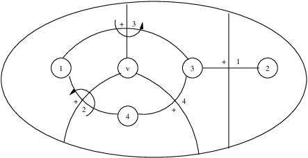
Now we can explain how to draw leaves of the foliation on the disc. Consider the first index of the $(P-N)$-cycle, say $j_{1}$: look for the first letter of $EW(D)$ in which that index occurs: say $(j_{1},j_{2})^{\pm 1}$ (or $(j_{2},j_{1})^{\pm 1}$). Draw the two positive vertices and the singular leaves joining them, and label the vertices with their numbers and the saddle with its sign and number (see Figure 1). Then look for the (cyclically) next letter containing $j_{2}$: if it is a different one, then draw it attached to the previous one (see Figure 2), if it is the same letter, then procede to the next letter containing $j_{1}$. We have to run twice through each $aa$-saddle.

To respect embeddability, when a positive vertex has two or more saddles attached, and we have to draw another one attached to it, we must put it in the right (counterclockwise) cyclic order about the vertex (see Figure 3).

Procede as indicated above until you get back to $j_{1}$ and the $(P-N)$-cycle is completed. These singular leaves divide the disk into an outer part, which is connected to the boundary, and some inner parts, in which the negative vertices lie along with possibly those positive vertices which at this stage have not yet been drawn (see Figure 4). They are vertices occurring in the 1-cycles of the permutation. For each of them, draw its cycle of saddles in a similar way (see Figure 5), then attach it inside the appropriate inner region.

It remains to add the negative vertices. Look at the code of the disc, and put each negative vertex in its place, joining it to the (already existing) saddles by the other singular leaves (see Figure 6).

If $EW=(6,5)(5,4)\overline{(4,2)}(3,1)(5,3)(4,2)$, we can draw all the disc and see that the negative vertex must be either $0.1$ or $5.1$. But neither of them is embeddable: they both pass the first part of embeddability test, but not the $b$-arc test: in the first case, in $(4,5)$ we have $gb(3,5)$ interlocking with $b(4,0.1)$; in the second case we have for instance in $(3,4)$ $gb(3,5)$ interlocking with $b(4,5.1)$.

In a disc without negative vertices, condition (3) of Theorem 1.4 is vacuous, because there are no negative vertices, and so there are no $b$-arcs. This means that the embeddability test is considerably simpler for positive words than for arbitrary words, because the difficult part is the test for $b$-arcs.

As we anticipated in the remark at the end of the previous section, a good word completely determines the embedding of its disc. Indeed, a description of this embedding is computed by our GAP procedure GenerateDiscBoundary($n,W$).

To follow the program of Theorem 1.6 we first need to list all the positive discs, that correspond to all the positive good words. But since we are interested in conjugacy classes of braids, we can reduce a lot of redundancy at this stage by some easy conjugations. The following definition concerns all embeddable discs (not only the positive ones).

It is clear that two equivalent discs are isotopic. That is, not only are their boundary words equivalent as cyclic words, but in fact the entire singular foliation is the same, up to a cyclic permutation of the ‘names’ of the vertices and saddles.

We call them ‘easy conjugations’ because it is very easy and inexpensive to perform them on a computer (see the Appendix).

So for a given $n$ we will list all good words up to easy conjugations and inversions: see Proposition 12. We have written a function in GAP called EnumeratePositiveGoodWords($P$) that enumerates one representative for each orbit of the action of the group $G=S_{P}\times S_{P-1}$ on the set of positive words of $B_{P}$ with length $P-1$, where $S_{P}$ acts on the $P$ indices and $S_{P-1}$ acts on the letters of the word, discarding those which have not the required permutation property.

Once we have all positive good words up to easy conjugations, we can list all positive good words up to inversion by choosing $1,2,\ldots\lfloor\frac{P-1}{2}\rfloor$ letters of each word to become negative. This is done by another easy procedure, called EnumerateGoodWords$(P)$. Remember that words with different exponent sum are surely non conjugate.

For instance, the result of EnumerateGoodWords(4) is a list of 32 good words of exponent sum 3 or 1. We will get 32 other good words of exponent sum $-3$ and $-1$ by inversion. Notice that among these 64 good words, some represent the same braid, because it is possible to apply some relations: for instance $(2,1)\overline{(3,1)}(4,3)=(2,1)(4,1)\overline{(3,1)}$, and both words appear in the list; but notice that $(2,1)(3,1)(4,3)\neq(2,1)(4,1)(3,1)$, also both appearing in the list. So we cannot reduce the list also by relations, both because relations are different on words with different signs, and they are not easy to be performed by the computer.

S. J. Lee has reduced the 32 good words up to conjugation: there are three conjugacy classes with exponent sum 3, with representatives $(2,1)(3,1)(4,1)$, $(2,1)(3,1)(4,2)$ and $(2,1)(4,2)(3,1)$. There are four conjugacy classes with exponent sum 1, with representatives $\overline{(2,1)}(3,1)(4,1)$, $\overline{(2,1)}(4,1)(3,1)$, $\overline{(2,1)}(3,1)(4,2)$ and $(2,1)(4,2)\overline{(3,1)}$.

The process of inserting an $ab$-tile in a given foliated disc $D$ is explained well in [2]. The idea is to take another small disc $T$ (see Figure 8), with a negative vertex $v$ and a saddle $s$ inside it, and a distinguished arc $\alpha^{\prime}$ on its boundary $\partial T$, such that the four branches of $s$ end one in $v$, two in $\alpha^{\prime}$ and the fourth in $\partial T\setminus\alpha^{\prime}$. Then choose an insertion arc $\alpha$ along the boundary $\partial D$ and attach $T$ along $\alpha$ by identifying $\alpha$ with $\alpha^{\prime}$ (see Figure 9), and continue branches of saddles of $D$ ending in $\alpha$ inside $T$ till they arrive at $v$, and continue the two branches of $s$ ending in $\alpha^{\prime}$ inside $D$ till they arrive at two specified positive vertices of $D$. Get a new foliated disc $D^{\prime}$ in such a way that this is still embeddable.

We know the conditions for embeddability from Theorem 1.4, so we can impose conditions on the choice of the insertion arc $\alpha$, on the position of $v$ in the new vertex string of $D^{\prime}$, and the position of $s$ in the new saddle list of $D^{\prime}$, so that at least the first two conditions of embeddability are satisfied.

We remark that there is another reduction of redundancy studied in [2], which is the requirement that all $b$-arcs be essential: We say that a foliated disc is essential if a negative vertex is never attached by a saddle to a positive vertex which is adjacent to it in the vertex string. If it was inessential, we could reduce the foliation of the disc by eliminating that negative vertex and the saddle attaching it to an adjacent positive vertex, without altering the embeddability of the disc and the boundary braid. So from now on we will discard all inessential discs. Since the test for essentiality is very easy, this is a very inexpensive way to reduce redundancy in our list. After we have tested the first two embeddability conditions and eliminated inessential $b$-arcs we will run the third text for embeddability in Theorem 1.4.

In order to keep track of the information necessary for a possibly essential embeddable insertion, we have invented another combinatorial description of the disc $D$, also suitable for our implementation. We will code our disc $D$ by two sets: the cyclically ordered set of boundary points of saddles, read counterclockwise along $\partial D$, and the set of $bb$-saddles. The reader might like to compare what follows with Figure 6. Each $aa$-saddle has two points on the boundary $\partial D$, that we will call points of type Q; each $ab$-saddle has one point on $\partial D$ that we will call points of type R; and each $bb$-saddle lies entirely in the interior of $D$, with no point on $\partial D$.

With each boundary point we will associate: the sign of the attached saddle (overline points corresponding to negative saddles); the ordered list of two or three vertices to which the saddle is attached, and the ordinal number of the saddle.

The double index of $Q_{i,j}$ (or $\overline{Q}_{i,j}$) is such that the cyclic counterclockwise order about the saddle of the boundary point and the two vertices is $i,Q,j$.

The triple index of $R_{i,v,j}$ (or $\overline{R}_{i,v,j}$) is such that the cyclic clockwise order of this point and the three vertices around the saddle is $R,i,v,j$ (in particular, the central index is the negative vertex).

We call initial and final vertex of a boundary point respectively the first and the last positive vertex, as they occur as indices of the point. In the sequence read along the boundary, two consecutive points always have the final vertex of the preceding point equal to the initial vertex of the following point.

Each $bb$-tile can be coded by: the sign of the saddle, the ordered sequence of the four vertices around it, and its ordinal number.

These combinatorial data are clearly in bijective correspondence with the set of data given in Section 2, so they are sufficient to draw the foliated disc and to read the extended boundary word (cf [2]).

For instance, the disc of Section 2 is described by (cf Figure 6)

We code an insertion arc $\alpha$ by listing all the consecutive points of type Q and R contained in $\alpha$. The position of the new inserted negative vertex $v$ can be found as follows:

• •

  for each point $Q_{i,j}$ or $R_{i,u,j}$ in $\alpha$: if $j-i\leq 2$(mod $n$), then the insertion is inessential; otherwise we get $i+1<v<j-1$;

• •

  for each point $\overline{Q}_{i,j}$ or $\overline{R}_{i,u,j}$ in $\alpha$: if $i-j\leq 2$(mod $n$), then the insertion is inessential; otherwise we get $j+1<v<i-1$.

These conditions correspond to the cyclic order of vertices around saddles. This means also that if $\alpha$ contains more than one point, we have to intersect conditions coming from different points: if the intersection is empty, the insertion is not embeddable. We can list all possible intervals of insertion in order of increasing length (that is the number of singular boundary points), giving for each of them the possible essential position of the new negative vertex. If some of the two preceding conditions eliminate some arc $\alpha$ of length $k$, then all arcs with length greater than $k$ and containing $\alpha$ are inessential or not embeddable for the same reason. The complete list is done by our GAP procedure GetInsertionArcs($n,\partial D$).

In our example (see Figure 6), an insertion arc is for instance $\alpha=\{\overline{R}_{7,0.1,3},$ $R_{3,0.1,8}\}$, with $4<v<6$ from the first point and $4<v<7$ from the second, hence it must be $4<v<6$.

An insertion arc $\alpha$ has an initial and a final vertex $(i(\alpha),f(\alpha))$, respectively the initial vertex of its first point, and the final vertex of its last point. In our example they are $(7,8)$.

To know at which level $x$ the new saddle can be located, we need to look at levels of points of $\alpha$ and to consider the cyclic order of all saddles around the new vertex, and around the two positive vertices $i(\alpha),f(\alpha)$ (see Figure 10).

Suppose $\alpha=\{P_{1}(l_{1}),P_{2}(l_{2}),\ldots P_{N}(l_{N})\}$, where each $P_{j}$ can be either of Q or of R type, either positive or negative, and each $l_{j}$ indicates its level. Then we must have $l_{1}<l_{2}<\cdots<l_{N}<x$ (in cyclic order). Now we have to look for the point on $\partial D$ immediately preceding $P_{1}$ and containing the index $i(\alpha)$: suppose $y_{1}$ is its level: then we must have $y_{1}<x<l_{1}$. Also we have to look for the point on $\partial D$ immediately following $P_{N}$ and containing the index $f(\alpha)$: suppose $y_{N}$ is its level: then we must have $l_{N}<x<y_{N}$.

In our example: $6<13<x$, that means $13<x<6$, is the first requirement; $l_{1}=1$ and $l_{N}=5$, therefore $1<x<6$ and $13<x<5$. Intersecting these cyclic intervals we get $1<x<5$.

The sign of the new saddle only depends on the relative position of $i(\alpha),v,f(\alpha)$:

• •

  if $f(\alpha)<v<i(\alpha)$ then $s$ is positive;

• •

  if $i(\alpha)<v<f(\alpha)$ then $s$ is negative;

therefore the possible range of $v$ obtained before can be divided in two parts, giving different signs for $s$. Our GAP procedure GetSaddles($n,P+N-1,\partial D)$ gives all these results.

In our example, $f(\alpha)=8<4<v<6<7=i(\alpha)$ hence $s$ is positive.

At this stage, before proceeding with the expensive $b$-arcs test, we can perform an easy permutation test: when we do an insertion, it is easy to see how the corresponding extended word changes: a new saddle $[\pm 1,[i(\alpha),v,f(\alpha))],x]$ is inserted, this corresponds to inserting a new letter $(i(\alpha),f(\alpha))^{\pm 1}$ (or $(f(\alpha),i(\alpha))^{\pm 1}$) at the same level of $EW$: we get a longer word, which still must satisfy conditions given in Proposition 3 for an extended word. So we can try all possible combinations of $[\pm 1,[i(\alpha),v,f(\alpha))],x]$ and check the corresponding permutation, to discard the impossible ones.

For instance our possible insertions for the chosen arc $\alpha$ are $[+1,[7,v,8],x]$, with $x$ ranging between 1 and 5. So the new word might be one of the following:

For them we find the following permutations:

(the same for all, since $(8,7)$ commutes with second, third and fourth letters), which satisfies all conditions required by Proposition 3.

Now we have to perform the test for $b$-arcs. For this we need both $\partial D$ and the set of $bb$-saddles. Also, we first need to see how the code changes after an insertion.

• •

  if $i<v<i+1$ and in the same interval there are other existing negative vertices, we have to decide (by the embeddability test) the exact order of them in this interval, and rename old vertices in it if necessary;

• •

  if $y-1<x<y$, put $x=y$ and for any saddle which was at level $z\geq y$ put it at level $z+1$;

• •

  substitute $\alpha$ by $R^{sign(s)}_{i(\alpha),v,f(\alpha)}$;

• •

  for each point $Q^{\varepsilon}_{i,j}$ in $\alpha$, its other corresponding $Q^{\varepsilon}_{j,i}$ becomes $R^{\varepsilon}_{j,v,i}$;

• •

  each point $R^{\varepsilon}_{i,u,j}$ in $\alpha$ becomes a $bb$-saddle $[\varepsilon,[i,u,j,v]]$.

If for instance we make the insertion of $[+1,[7,4.1,8],4]$ on the chosen $\alpha$, the description of the new disc is (see Figure 9):

If a negative vertex $v$ (yet existing or newly inserted) is attached to more than two saddles (for the new vertex, this corresponds to an insertion arc of length greater than or equal to 2), we have to list these saddles in cyclic order about $v$ (in our example, they are $[7,4.1,8](4)$, $\overline{[7,0.1,3,4.1]}(7)$, $[3,0.1,8,4.1](14)$); between any two consecutive of them, find the $b$-arc between $v$ and the only other positive vertex which is in common for the two saddles (in our example: in $(4,7)$ have $b(7,4.1)$; in $(7,14)$ have $b(3,4.1)$; in $(14,4)$ have $b(8,4.1)$).

As explained in [2], we have to compose an array with: in the first column the $P+N-1$ intervals $(k,k+1)$ between two consecutive saddles; in the following $N$ columns, the $b$-arcs for each negative vertex in the corresponding intervals; in the last column, the $gb$-arcs (they are as many as the $aa$-saddles). For instance, for our new disc of Figure 9 we see the array of Figure 12.

It is necessary that along each row of the array the arcs which appear do not interlock with each other. All these checks are performed by our GAP procedure Embeddable$(n,P+N-1,\partial D,bb$-saddles). Finally, our GAP procedure InsertVertices$(n,P+N-1,\partial D,bb$-saddles, depth) recursively tries all possible insertions of $ab$-tiles and returns all the resulting new embeddable essential tiled disc.

To get the boundary word $BW$ we have to eliminate from $EW$ the $N$ strands corresponding to the $N$ unlinked circles about each negative vertex. In this way, from each letter of $EW$ we will get a new letter or subword of the boundary braid $BW$, which is a braid of $B_{P-N}$.

To do so, let us introduce some useful braids (called descending cycles in [3]):

Notice that $\delta_{p,p-1}=(p,p-1)=\sigma_{p-1}$. The associated permutation is $\rho(\delta_{p,q})=(q,q+1,\ldots,p)$.

The strands to be eliminated are numbered, at the beginning of $EW$, by the $N$ 1-cycles of $\rho(EW)$. At each letter of $EW$ their numbers might change, as can be seen for instance in Figure 13. The rule is: suppose $L_{k}=\{i_{1},i_{2},\ldots i_{N}\}_{k}$ is the list of levels of strands to be eliminated just before the $k^{th}$ letter of $EW$, and this letter is $(h,j)^{\varepsilon}$ (see Figure 14):

1. 1.

   if both $h,j$ are not in $L_{k}$, and $h^{\prime},j^{\prime}$ are the numbers of elements of $L_{k}$ which are less than $h,j$ respectively; then get $(h-h^{\prime},j-j^{\prime})^{\varepsilon}$; $L_{k+1}=L_{k}$;

2. 2.

   if $j\in L_{k}$ and $h$ is not in $L_{k}$: if $h>j+1$, then get $\delta_{h-h^{\prime},j-j^{\prime}}$; if $h=j+1$, then get the empty word $e$; $L_{k+1}=(L_{k}\setminus\{j\})\cup\{h\}$;

3. 3.

   if $h\in L_{k}$ and $j$ is not in $L_{k}$: if $h>j+1$, then get $\delta^{-1}_{h-1-h^{\prime},j-j^{\prime}}$; if $h=j+1$, then get $e$; $L_{k+1}=(L_{k}\setminus\{h\})\cup\{j\}$;

4. 4.

   if both $h,j\in L_{k}$, then get $e$; $L_{k+1}=L_{k}$.

References

- [1] J. S. Birman, E. Finklestein, Studying surfaces via closed braids, Journal of Knot Theory and its Ramifications, vol. 7, n. 3 (1998) 267–334.
- [2] J. S. Birman, M. D. Hirsch, A new algorithm for recognizing the unknot, Geometry and Topology, 2 (1998) n. 9, 175–220.
- [3] J. S. Birman, K. H. Ko, S. J. Lee, A new approach to the word and conjugacy problems in the braid groups, Advances in Mathematics, 139 (1998), pp. 322–353.
- [4] J. S. Birman, K. H. Ko, S. J. Lee, ”The infimum, supremum and geodesic length of a braid conjugacy class”, preprint arXiv:math.GT/0003125
- [5] J. S. Birman, W. Menasco, Studying links via closed braids IV: composite links and split links, Inventiones math. 102 (1990), 115-139.
- [6] J. S. Birman, W. Menasco, Studying links via closed braids V: the unlink, Transactions A.M.S. 329 (1992) 585–606.
- [7] T. Fiedler, A small state sum for knots, Topology 32, No. 2 (1993), 281-294.
- [8] H. Goeritz, Bemerkunger zur Knotentheorie, Hamburg Abhandlungen 10 (1934), 201-210.
- [9] Graphlet: A toolkit for graph editors and graph algorithms, Faculty of Mathematics and Computer Science, University of Passau, http://www.infosun.fmi.uni-passau.de/Graphlet/.
- [10] W. Haken, Theorie der Normalflachen, Acta Math. 105 (1961) 245–375.
- [11] J. Hass, Algorithms for recognizing knots and links, preprint arXiv:math.GT/9712269
- [12] J. Hass and J. Lagarias, The number of Reidemeister moves needed for unknotting, arXiv:math.GT/9807016
- [13] J. Hass, J. Lagarias and N. Pippenger, The computational complexity of knot and link problems, preprint arXiv:math.GT/9807016
- [14] J. Hoste, M. Thistlethwaite and J. Weeks, The first 1,701,936 knots, The Mathematical Intelligencer, 20, No. 4 (1998), 33–48.
- [15] W. Jaco and J.L.Tollefson, Algorithms for the complete decomposition of a closed 3-manifold, Ill J. Math 39 (1995), 358-406.
- [16] D. B. Johnson, Finding all the elementary circuits of a directed graph, SIAM J. Comput. 4 (1975) 77–84.
- [17] E.S.Kang, K. H. Ko, S. J. Lee, Band presentation for the 4-braid group, Topology and its Applications 78 (1997) 39-60.
- [18] H. Kneser, Geschlossene Flachen in dreidimensionalen Mannigfaligkeiten, Jahresbericht Math. Verein. 28 (1929), 248-260.
- [19] K. H. Ko, S. J. Lee, Genera of some closed 4-braids, Topology and its Applications 78 (1997) 61–77.
- [20] S.J. Lee, Implementation of an algorithm for solving the conjugacy problem in the braid groups. sangjin@knot.kaist.ac.kr
- [21] W. Magnus and A. Pelluso, On a theorem of V.H.Arnold, Com. on Pure and Applied Math., XXII (1969), 683-692.
- [22] H. R. Morton, Exchangeable Braids, Low–dimensional Topology, London Math. Soc., 1982, Lecture Notes in Science vol 95, ed. R. Fenn, pp. 86–105.
- [23] H. R. Morton, Threading knot diagrams, Math. Proc. Cambridge Phylos. Soc. 93 (1983) 247–261.
- [24] H. R. Morton, An irreducible 4–braid with unknotted closure, Math. Proc. Camb. Phil. Soc. 93 (1993) 259–261.
- [25] M. Rampichini, Exchangeable fibred links, doctoral thesis, february 1998, Milano, Italy.
- [26] L. Rudolph, Quasipositive plumbing (Constructions of quasipositive knots and links, V), Proc. AMS 126 (1998) 257–267.
- [27] F. Ruskey, J. Sawada, An Efficient Algorithm for Generating Necklaces with Fixed Density, SIAM J. Comput., 29 (1999) 671–684.
- [28] P. Vogel, Representation of links by braids: a new algorithm, Comm. Math. Helv., 65 (1990) 104–113.
- [29] G. Wright, A foliated disk whose boundary is Morton’s irreducible 4-braid, preprint, March 1998.
- [30] S. Yamada, The minimal number of Seifert circles equals the braid index of a link, Invent. Math. 89 (1987), 347–356.
Joan S. Birman, Dept.of Mathematics, Barnard College
Mail Code 4427, Columbia University
2990 Broadway, New York, N.Y., USA 10027
e-mail: jb@math.columbia.edu
Marta Rampichini,
Dipartimento di Matematica
Università di
Milano
via Saldini 50, 20133, Milano, Italy
e-mail: rampichini@mat.unimi.it
Paolo Boldi and Sebastiano Vigna, Dipartimento di Scienze
dell’Informazione
Università di Milano
via Comelico 39/41, 20135 Milano, Italy
e-mail: {boldi,vigna}@dsi.unimi.it