Maximal Singular Loci of Schubert Varieties in Thanks: Work supported by NSF grant DMS-9983797
Abstract.
Schubert varieties in the flag manifold play a key role in our understanding of projective varieties. One important problem is to determine the locus of singular points in a variety. In 1990, Lakshmibai and Sandhya showed that the Schubert variety is nonsingular if and only if avoids the patterns and . In this paper we give an explicit combinatorial description of the irreducible components of the singular locus of the Schubert variety for any element . These irreducible components are indexed by permutations which differ from by a cycle depending naturally on a or pattern in . Our description of the irreducible components is computationally more efficient () than the previously best known algorithms, which were all exponential in time. Furthermore, we give simple formulas for calculating the Kazhdan-Lusztig polynomials at the maximum singular points.
1991 Mathematics Subject Classification
14M15 (Primary); 05E15 (Secondary)1. Introduction
Schubert varieties play an essential role in the study of the homogeneous spaces for any semisimple group and Borel subgroup ; every closed subvariety in can be written as the union of Schubert varieties, the classes of Schubert varieties form a basis for the cohomology ring of and the Schubert varieties correspond to the lower order ideals of a partial order associated to . Specifically, this Bruhat order is an order on the -fixed points in where is the maximal torus in . The -fixed points, , correspond bijectively with elements in the Weyl Group of and . A tremendous amount of information about a Schubert variety can be obtained by examining the corresponding Weyl group element. Our main theorem gives a simple and efficient method for giving the irrducible components of the singular locus of a Schubert variety11 1 While in the process of preparing this submission, the authors have learned that Manivel [Man01] has recently independently proved a theorem equivalent to Theorem 1..
In the late 1950’s, Chevalley [Che94] showed that all Schubert varieties in are nonsingular in codimension one. Since that time, many beautiful results on determining singular points of Schubert varieties have surfaced (see [BL00]). By definition, the Schubert variety is the closure of the -orbit of . Therefore any point is singular if and only if all points in the orbit are singular. Since the singular locus of a variety is closed, the singular locus of is a union of Schubert varieties indexed by the maximal elements such that is singular in .
Let denote the maximal set of Weyl group elements corresponding to singular points in in Bruhat order, i.e. is an irreducible component of the singular locus of if and only if . The goal of this paper is to give an explicit algorithm for finding in the case where is , is the set of invertible upper triangular matrices, is the set of invertible diagonal matrices, and is the symmetric group . The algorithm we present is very efficient, , and removes the need to search through all nonsingular -fixed points (as is the case with previously known techniques).
In type (i.e., ), smoothness is equivalent to rational smoothness ([Deo85], see also [CK99] in the case of ) so the maximal singular locus of also determines the maximal permutations for which the corresponding Kazhdan-Lusztig polynomial is different from 1. We use the explicit form of to compute all Kazhdan-Lusztig polynomials at maximal singular points (msp’s); they are either or depending on whether the corresponding bad pattern is or (respectively).
2. Main results
In 1990, Lakshmibai and Sandhya [LS90] showed that the Schubert variety is smooth at every point if and only if the permutation matrix for does not contain any submatrix equal to or . We use these two permutation patterns to produce the maximal permutations below which correspond to points in the singular locus. This verifies the conjecture stated in [LS90]. (Gasharov, using a map similar to the one we introduce in Section 6, shows in [Gas00] that the points constructed in [LS90] are singular. His result proves one direction of this conjecture.) In fact, our proof starts from an arbitrary maximal singular -fixed point in and shows that must contain a or pattern and must contain a or pattern (respectively).
The main theorem below shows that elements of are obtained by acting on by certain cycles. These cycles, described in the following theorem, are best absorbed graphically in terms of the permutation matrices and . Examples are shown in Figures 1 and 2.
Theorem 1.


After introducing basic notation in Section 3, we then introduce in Section 4 the pictorial characterization of the Bruhat order we rely on. In sections 5 and 6, we discuss the Lakshmibai-Seshadri basis for the tangent space of a Schubert variety indexed by transpositions and the set . We also define a set of maps that allows us to relate and when and differ by a transposition. These maps will then allow us to investigate not only whether a point is singular, but whether it is maximally singular. To describe those permutations , we show that related permutations must, among other qualities, avoid the patterns , and . We complete the description of in sections 8,9 and 10.
The remaining sections contain applications arising from our description of . In Section 11, we prove the conjecture of Lakshmibai and Sandhya on the composition of . Using the tools we have developed, in Section 12 we calculate the values of the Kazhdan-Lusztig polynomials at maximal singular points. In Section 13, we give some example calculations pertaining to the composition of . Finally, in Section 14, we state a simple method for determining the number of elements in in terms of pattern avoidance and containment.
3. Preliminaries
We begin by introducing our basic notation and terminology. Let denote the symmetric group on letters. We will view elements of as permutations on . To this end, we identify with the transposition . Let be the image of under the permutation . We have a one-line notation for a permutation given by writing the image of under the action of : . We will also often utilize the permutation matrix for (denoted ).
We use the standard presentation
| (3.1) |
Let denote the generating set for . Let denote the set of all transpositions in . The elements of are all the conjugates of elements in :
| (3.2) |
If we wish to refer to a transposition that affects positions and , but the relative values of and are unknown, we will write .
An expression is any product of generators . The length of an element is the minimum for which we have an expression . A reduced expression is an expression for which . It is a standard fact that
| (3.3) |
Definition 2.
Let , . Define the rank function for by . Also, the difference function for the pair is defined by .
In , Schubert varieties can be defined in terms of the rank function. To do this, fix a basis of . This fixes a base flag where is the span of . We identify with the set of all complete flags of vector spaces with . Then
| (3.4) |
(This definition is equivalent to that given in [Ful97].) Note that the flag
| (3.5) |
is an element of . Furthermore, is fixed by the left action. Also, since can be viewed as the closure of the orbit , if and only if . This defines a partial order, called the Bruhat (or Bruhat-Chevalley) order on by
| (3.6) |
The Bruhat order has a number of characterizations (see, e.g., [Hum90]). One of the most common definitions is as the transitive closure of the relations for if . However, we prefer to work with a more graphical characterization which follows directly from the definition of the rank and difference functions above. The corresponding “Bruhat pictures” that we associate to each pair will be discussed in the next section. These pictures will rely on the below two conclusions.
Lemma 3.
We have if and only if is everywhere non-negative.
Corollary 4.
If , then is everywhere non-negative.
The Bruhat graph of is the graph with vertices labeled by and is joined to by a directed edge if for some and in Bruhat order. This graph plays a central role in the study of Schubert varieties. For example, Lakshmibai and Seshadri have shown that in , the tangent space to at has a basis indexed by , i.e. the edges of the Bruhat graph adjacent to . This fact forms the main criterion we will use in Section 5 for smoothness at a point. In fact, since implies we will just need to consider the edges “going up” from in the Bruhat graph of . As mentioned in the introduction, this set will be denoted by
Over the last few years, it has become apparent that properties of the Bruhat order can often be efficiently characterized by “pattern avoidance” [BL98, Ber92, BW, LS85, Ste96]. We say that avoids the pattern for if we cannot find with in the same relative order as - i.e., no submatrix of on rows and columns is the permutation matrix of . Our characterization of the maximal singular locus is yet another example of the utility of this notion.
More generally, we can define pattern avoidance or containment in terms of the following flattening function. For any set , and , define to be the “flattened” permutation on whose elements are in the same relative order as . When the set is clear from context, we will abbreviate by . We will also write for the flattened permutation on the sequence and write for .
It will also be useful to have notation for an “unflattening” operator. Given a permutation , a set , and a permutation , we can define a new permutation by requiring that
- (1)
, and
- (2)
if .
When and are clear from context, we abbreviate by .
Example 5.
For and , we have and . Note that .
4. Bruhat pictures
Our main theorem is concerned not only with determining which points in a given Schubert variety are singular, but which are maximally singular. The function affords us a graphical view of the Bruhat order. Most importantly, it lets us see the set . We will now introduce the graphical notation utilized in the remainder of the paper that allows us to do this. A diagram displaying the notation we are about to describe is offered in Figure 3.

First, we plot, as black disks, all or some of the positions containing 1’s in the permutation matrix of . We will sometimes overlay and . In these cases, 1’s in will be marked by open circles. Points that are simultaneously in both diagrams will consist of a black disk and a larger concentric circle. Let denote the set of all points such that and . The following notation will be handy:
Definition 6.
For , set
| (4.1) | ||||
| (4.2) | ||||
| (4.3) |
Along with the points of , we will often shade parts of our diagram in order to specify that satisfies a particular inequality on a given region. Light shading on a region signifies that on that region. Dark shading signifies . No shading places no restrictions on the values . A region with a black border is one where achieves the minimum possible value allowed by the shading on that region. Dotted borders are used to demarcate regions we wish to discuss in the text.
As mentioned above, the great utility of these diagrams arises from being able to visualize along with the information on the Bruhat order. To see how we do this, suppose we have some reflection (which implies ). Now compare the shading (with respect to ) in and . We see (as in Figure 3), that in the region , . Hence, by Lemma 3, we can state the following:
Fact 7.
Let with . The transposition is in if and only if it corresponds to a region in that is entirely shaded (i.e., ). An example is given in Figure 4

Note that the values of on the region are not considered in determining the membership of in .
In order to highlight reflections that we are particularly interested in, we will often draw an arc in our diagram. A solid or dotted curve connecting two points in will denote an element of . A dotted curve will be used to designate when we are particularly interested in . A dashed curve will be used when we wish to mark a reflection . Of course, if , and our picture is of , then only one of the endpoints of our dashed curve will correspond to a point of . There are numerous instances when an arc corresponds to an element of . In this case, whether we use a solid or dashed arc depends on context.
The following lemma will be used several times in future sections. It allows us to infer the presence of points in in a region based on a particular common pattern of shading.
Lemma 8.
Let and suppose such that
- (1)
, ,
- (2)
,
- (3)
, , .
Then there exist at least values such that with .
Proof.
Let’s define four regions as follows:
- •
,
- •
,
- •
,
- •
.

For every subset , define
| (4.4) |
Then
Now,
| (4.5) | ||||
| (4.6) |
So and there are exactly more 1’s of than 1’s of in region . This finishes the proof. ∎
5. A criterion for maximal smoothness
To prove Theorem 1, we start from the fact that (by definition) is smooth at if and only if the dimension of the Zariski tangent space at that point is equal to . Lakshmibai and Seshadri, [LS84], describe the dimension of this tangent space in terms of the root system. Using the fact that , we can paraphrase their result as:
Theorem 9.
[LS84] The Schubert variety is smooth at if and only if equals .
This yields the following characterization of the permutations in :
Fact 10.
if and only if
- (1)
and
- (2)
for all , .
As may be ascertained from Theorem 1, the criteria for to be an element of are local in nature. This implies that we may concentrate on only certain indices in our permutation in order to determine . We now describe these indices explicitly.
Definition 11.
Let
| (5.1) |
For , set
| (5.2) | ||||
| (5.3) |
Note that and are permutations in .
We state here for reference the following useful characterization of .
Corollary 12.
Let . Then and if and only if .
We now give a sufficient condition for an index to be in .
Proposition 13.
Suppose and with .
- (1)
If , then with and .
- (2)
If , then with and .

Proof.
First we prove the case of . Note that
| (5.4) |
since . Let . Choose as large as possible such that and (see Figure 6). Such a must exist since . Now choose as small as possible such that and for all with . Then there exists a , such that . By construction,
That is (in the notation of Lemma 8), , and . So by this lemma, there exists an such that and . Then , so by Fact 7, . This proves our claim.
To prove the case of , it is easiest to use dual rank and difference functions:
| (5.5) | ||||
| (5.6) |
One can check that if and only if and then argue as above using this new rank function. (Note, to define using , we have to modify our fixed flag and (3.4).) ∎
Corollary 14.
If and , then there exists with .
Proposition 13 tells us that if then . It turns out that the question of whether or not depends only on the pair . This is borne out by the following simple facts. They will be used without comment in the remainder of the paper.
Lemma 15.
We have the following:
- (1)
If , then .
- (2)
.
Proof.
The first equivalence follows from Lemma 3 by comparing and . The second follows from the first by noting that whenever . ∎
Proposition 16.
We have the following:
- (1)
.
- (2)
There exists a bijection .
- (3)
if and only if .
6. The Map
In Fact 10 we claimed that can be identified in terms of for . To do this, we will need to relate to when differ by an element of . So, for every triple with , we will define a map . In Theorem 21 we will show that the image is actually contained in . The values of are usually clear from context and we will often abbreviate as . Propositions 26, 27 and 29 contain interesting implications of the map .
A similar map has been defined by Gasharov [Gas00] for the purpose of showing that certain elements constructed by Lakshmibai and Sandhya in [LS90] are, in fact, singular points. See Section 11 for details.
Definition 17.
Fix . Given some , if and commute, we define . Otherwise, we can find such that implies . Then we define according to Table 1.
| Case | |||||||
|---|---|---|---|---|---|---|---|


Remark 18.
It is not sufficient to define . For example, in the situation of Case C.ii, where and , we have .
Example 19.
In order to elucidate the definition, we give here several example of the map . Let and . We see that (see Figure 9.1).

Remark 20.
It is possible for for and . For example, let , and . Then and .
It is clear from the definition that is always a reflection and that . But for to be useful, we will need the following property.
Theorem 21.
Fix . The map is injective.
For the proof of this theorem, we’ll need the following simple lemma.
Lemma 22.
Let and suppose such that . If both
| (6.1) | ||||
| (6.2) |
then (i.e., ).
Proof.
Notice that for and for . By Lemma 3, if and only if . Since , . Combining this with our first observation implies that . ∎
Now we are ready to prove Theorem 21.
Proof.
First we show that — i.e., for all . It is clear from the definition that . So this amounts to showing that one of the two dotted arrows in Figure 10 (corresponding to relation under the Bruhat order) exists.
First suppose — hence . We wish to show that . Letting and , this reduces to showing that . Now implies that . So if . But this last inequality holds by choice of .
Now suppose that . In all of the cases in Table 1 except A.iii and B.iii, . Since and agree at all indices except , we can use Lemma 15 to conclude that . So for all cases except possibly A.iii and B.iii.
In Case A.iii, we know that both , — i.e., . Since and , we can therefore invoke Lemma 22 to conclude that . Case B.iii is similar.
It is clear from Table 1 that can share at most one index with . As we have already shown the inclusion , we conclude that .
Now we show that is an injection. Suppose , . No matter which case of Table 1 we are in, we see that or . In other words, the index doesn’t share with must be an index of . In particular, if such that , the index they don’t share with must be the same. It is then easy to check by inspection of Table 1 that implies that . Since whenever and don’t share any indices, we conclude that is, in fact, an injection. ∎
The above theorem has as a simple corollary a special case of Deodhar’s conjecture [Deo85].
Corollary 23.
.
Various forms and generalizations of the preceding corollary have been proven by Dyer [Dye93] (arbitrary Coxeter systems), Deodhar [Deo85] (type A), Polo [Pol94] (finite Weyl groups) and Carrell-Peterson [Car94] (crystallographic groups).
Corollary 24.
For , implies that .
Next, we see that when is an adjacent transposition with , surjects onto . It would be interesting to classify all such for which this happens.
The following fact about the Bruhat order will in useful in the proof of the next proposition and later in the paper. An analogous left-handed version exists.
Lemma 25 ([Hum90],Lemma 7.4).
If and , then .
Proposition 26.
Let (i.e., is an adjacent transposition) and suppose satisfy the relations with . Then and is smooth in if and only if is smooth in .
Proof.
The last statement follows immediately from the decomposition of . So, taking advantage of Theorem 21, we need only show that if , then .
First consider the case where . Then . As , we can apply Lemma 25 to conclude that . Finally, since , . So in this case.
Now, as in the proof of injectivity, we can restrict to the cases where . We group into cases according to , and . Cases have ; Cases have . In each case we show that .
| Case | |||||
|---|---|---|---|---|---|
| Since , and . So we are in Case A.iii and we see that . | |||||
| Case B.iii — analogous to I. | |||||
| By Lemma 25, if and only if . The latter inequality is true since . So . We’re in Case A.i and . | |||||
| Case B.i — analogous to III. | |||||
| . Hence, by Lemma 22, . So . We’re in Case C.i and . | |||||
| Case D.i — analogous to V. |
Cases I-VI are the only ones possible since cannot have as hypothesized. ∎
Proposition 27.
Let (i.e., is an adjacent transposition) and suppose satisfy the relations with . Then .
Proof.
By Proposition 26, . The result follows from the identity . ∎
Corollary 28.
If is an msp, any simple reflections, then or imply, respectively, that or .
The preceding corollary is well-known [BL00, 8.2.10]. However, Proposition 26 gives a different proof.
There is one more fundamental property of that we will need to know for the rest of the paper. Namely, for a pair of reflections where , it will be useful to know what we can say about the membership of in .
Proposition 29 (Reciprocity).
If , , with , then .
Remark 30.
Reciprocity does not necessarily hold if . For example, take , , and . Then but .
Proof.
Suppose . We will show that .
First, consider the case where . From the definition of , we see that . So . This implies that and therefore .
Now we suppose . So are determined such that implies . Let . Note that:
- (1)
By hypothesis, .
- (2)
If then at most one of ; not two.
Hence, the cases below are the only ones we need consider.
- (1)
- (2)
.
The argument is parallel to that in the previous case. - (3)
∎
7. Preparatory lemmas
The above fact is most conveniently expressed in terms of the following notation:
Definition 31.
For and , let
| (7.2) |
denote the set of “extra” reflections corresponding to and . We often write for .
If , then we say that and are incompatible edges (in the Bruhat graph). The elements of are “extra” edges in the sense that they correspond to an increase in the dimension of the Zariski tangent space.
The utility of is embodied in the following two facts.
Fact 32.
If with and , then is singular.
Fact 33.
is an msp for if and only if, for every with , .
Note, however, that if is a singular point, but not an msp, then it is possible that . An example is afforded by , and . Conversely, if , then we may have even if is entirely smooth. Take, for example, , , and .
There will be numerous instances in the remainder of the paper where we do the following:
- (1)
Assume we have an msp for .
- (2)
Construct some .
- (3)
Conclude that from the fact that is shaded.
- (4)
Find incompatible edges as in Fact 32 to conclude that is also a singular point of .
- (5)
Obtain a contradiction with our first assumption.
The previous technique will allow us to significantly pare down the possibilities for what looks like for an msp. The following lemma is the first example of this strategy.
Lemma 34 (Ell Lemma).
Let and .
- (1)
If and , then and .
- (2)
If and , then and .
Proof.
We only prove 1 as the proof for 2 is entirely analogous.
Diagrams for , and are given in
Figure 11.

The next lemma is used frequently. It gives us criteria for determining when two reflections are, in fact, incompatible.
Lemma 35.

Proof.
The proof of Patch Incompatibility is clear. To prove Link Incompatibility, it suffices to consider Cases A and B of Definition 17. ∎
In Fact 32 we give a sufficient condition for to be a singular point of that is expressed in terms of the map . Namely, is singular if is non-empty for some with . As the lemma below shows, many elements of aren’t even candidates to be elements of .
Lemma 36.
Let . If , then (i.e. — ).
Proof.
For any point , . Similarly for the pair and . Now, implies that and on . This implies that and . ∎
The following lemma is technically useful for Proposition 38.
Lemma 37.
Let , , , and . If or , then is not an msp for .
Proof.
First consider the case where both .

Suppose there is a point in region A of Figure 13.1. Choose such an as small as possible. Then we see that and are patch incompatible reflections for and . By Fact 32, is then singular. This contradicts the fact that is an msp for .
Now suppose region A of Figure 13.1 is empty — this is shown in Figure 13.2. Then and are incompatible reflections for and . Since , this contradicts the fact that is an msp for .
We now argue the case of . (The arguments for are parallel.)
Clearly and . There are four possibilities with regard to the position of .
- (1)
.
We are in Case A.iii of the definition of . Hence, , which is a contradiction. So this case cannot occur. - (2)
, .
This case cannot occur as it violates . - (3)
- (4)
, .
See Figure 14.2. This is analogous to the previous case.
Figure 14.
∎
Proposition 38 below gives us our first non-trivial restriction regarding the composition of . This proposition will greatly reduce the amount of work we need to do later on to determine possibilities for .
Proposition 38.
Let be an msp. If then .
Proof.
Suppose that and . We will obtain a contradiction.
Let . Choose as large as possible such that . Note that and . Since is an msp, we can invoke Fact 33 to find a .
Suppose . Since , is shaded so . Hence and are incompatible for and . This contradicts .
Otherwise, overlaps both and , so, by Lemma 37, we are in one of the following two scenarios.
- (1)
.
By choice of , . (Note that .) So either , or , (the latter case is shown in Figure 15.1.). In either case, we can apply the Ell Lemma 34 to conclude that . This contradicts the choice of .
Figure 15. - (2)
.
Since , for to be an element of , we need , and for some point in each of regions A and B in Figure 15.2. But then and are link incompatible for . Furthermore, by having chosen as large as possible, we ensure that . This contradicts .
∎
We are now able to give a graphical description of all possible pairs such that when . The result follows immediately from Lemma 36 and Proposition 38 along with the Ell Lemma 34. Note that by Proposition 29, we can assume, without loss of generality, that .
Corollary 39.
If and , then the relative positions of and are one of the ones shown in Figure 16.

This greatly simplifies our future investigations. We now use Corollary 39 and Lemma 8 to prove the following crucial lemma.
Lemma 40 (Cross Lemma).
Let be an msp and suppose such that . If and , then .
Proof.
We can visualize the situation as in Figure 17.1.

Since , there is necessarily a point in region A for which . Suppose . Then there is a point in region B such that . Then we can apply Lemma 8 (with , ) and Proposition 38 to conclude that there is a point of in region (see Figure 17.2). If we choose to be as low as possible in our diagram, then (see Figure 17.3). But then and are patch incompatible for . This contradicts . Therefore and we can shade the entire region B.
To shade the lower left corner, apply the preceding argument to and . ∎
8. Restrictions on
Recall that and are the restrictions of and to those positions in (see Definition 11). In order to determine the structure of , we first prove the following necessary conditions on for any msp for .
Theorem 41.
If is an msp, then is 231- and 312-avoiding.
Theorem 42.
If be an msp, then is 1234-avoiding.
These two theorems are, in fact, almost enough to describe for any msp .
8.1. Technical lemmas regarding
In order to streamline the proof of Theorem 41, we first present two technical lemmas. These lemmas simply show that , for an msp, must avoid certains patterns of points and shading.
Lemma 43.
If is an msp, then does not contain either of the configurations in Figure 18 (regardless of whether or not these reflections are incompatible).

Proof.
We only prove that must avoid the configuration in Figure 18.1. The proof of the other case is parallel.
First suppose that (see Figure 18.1). Then by the Cross Lemma 40, . But this contradicts Proposition 38 as . We get a similar contradiction if . So we can henceforce assume that our configuration is actually as in Figure 19 — i.e., , .

Since is an msp, we must have some reflection . Suppose
| (8.1) | ||||
| (8.2) |
In the case of (8.1), and are incompatible for . This contradicts . (Similarly for (8.2).) So these intersections must be non-empty. It is clear from Figure 19 that for these intersections to be non-empty, we need to be patch (rather than link) incompatible with each of , and . By Proposition 38 and because the intersections in (8.1) and (8.2) must be non-empty, it is readily seen that we require and . Hence, there are only four possible ways in which may overlap , and . These are shown in Figure 20.

- (1)
- (2)
, .
The argument is parallel to the previous case. - (3)
- (4)
, .
Here and are patch incompatible for . This contradicts .
∎

Proof.
Since is an msp for , there exists some . Clearly, if
| (8.3) |
then and are (patch or link) incompatible reflections for . This would contradict .
So, to ensure that (8.3) does not hold, we need in region A of Figure 22.1 and in region B. Here we are including the possibilities that or . Note that (as is shown in Figure 22.1) Proposition 38 requires that and . Clearly if then and vice versa. Hence, by symmetry, we can treat only the cases where . These two cases are illustrated in Figures 22.2 and 22.3.

8.2. Proofs of Theorems 41 and 42
Theorem 41.
By passing to inverses, it is enough to prove that is 231-avoiding. So choose with such that .

- (1)
Assume .
We have the situation of Figure 23.By definition of , there exists a with . We’ll assume that as all cases where are analogous to one of the cases we cover by transposing over the anitdiagonal. Clearly .
Since is an msp, there exists a . We claim that
(8.4) Suppose the intersection is empty. Then and are (patch or link) incompatible for . This contradicts . So we may assume that this intersection is non-empty. There are three cases according to whether and are
- (a)
link incompatible
- (b)
patch incompatible with .
- (c)
patch incompatible with .
We only describe the arguments explicitly in the case of link incompatibility — the arguments are similar in the latter two cases. We will argue only as the case of is analogous.
By Propositon 38, there are three possibilities for the relative positions of and . They are displayed in Figure 24.

Figure 24. - (a)
(i.e., ).
We have that and are link incompatible for . This contradicts . - (b)
(i.e., ).
The argument is the same as in the previous case. - (c)
- (a)
- (2)
Assume .
Since , we can find such that . If
Figure 25. - (a)
is in region A or A’ of Figure 25.1 or
- (b)
is in region C or C’ of Figure 25.2 or
- (c)
is in region E or E’ of Figure 25.3,
then we can reduce to the previous case (of ) or we violate Proposition 38. So we must have
- (a)
- (b)
- (c)
As the argument of is analogous, we will assume .
We now argue the four cases we have left according to whether and whether .

Figure 26. - (a)
- (b)
, .
Since is an msp, there exists some . As , one can see in Figure 26.2 that . Hence, and are (patch or link) incompatible for . - (c)
- (d)
- (a)
This completes the proof that is 231- and 312-avoiding. ∎
Theorem 42.
Suppose we have with and . We will obtain a contradiction.

Since , there exist such that . As is an msp, there also exists some . Using Proposition 38, it is easy to check that if
| (8.5) |
then and are incompatible for . This contradicts . So, in particular, . A typical (allowable) pair of positions for and is shown in Figure 27.2.
As we have now constructed with , we will assume that and were chosen initially such that . Note that by the above construction, we can assume that . Suppose . Then and ( or ) are link incompatible for . This contradicts .
So our diagram looks like that pictured in Figure 28.1 and we have .

Therefore, we can find a point in each of the regions U & V such that . Choose the point in region U to be as low as possible. Choose the point in region V to be as far right as possible. Such points are shown in Figure 28.2. Apply Lemma 8 to the rectangle determined by these two points with and . This, along with Proposition 38, implies that there is another point in either region P or Q. Without loss of generality, assume it is in region P. By having chosen the point in region U as low as possible, we find that (see Figure 28.3). Hence, and are link incompatible for . This contradicts . ∎
9. Restrictions on
Combining Theorem 41 and Theorem 42, we see that if , then
| (9.1) |
for some . If two out of three of are , then is strictly decreasing, so implies that . But then cannot possibly be an msp. So now we determine the possible values of in Proposition 45 when and the possible values of in Proposition 46 when . In each proposition, we also determine what must be to allow to be singular.
We know from Proposition 16 that if and only if . Hence, for the remainder of this section, we will only consider the case where and .
9.1. Two decreasing sequences in
Proposition 45.
Let with and . Suppose that consists of exactly two decreasing sequences:
| (9.2) |
for some . Then
- (1)
and
- (2)
(shown in Figure 33.3).
Proof.
For brevity in the following, we use the convention that and .
Condition 2: We split this proof into proving the following facts:
- (1)
.
- (2)
for all and .
- (3)
.
- (4)
is as in the statement of Condition 2.
We now prove these claims.
- Step 1.
.
Assume . We will obtain a contradiction.By Proposition 13, we can find such that (see Figure 29). Choose as large, as small as possible subject to this restriction.

Figure 29. If , then an application of the Cross Lemma 40 would offer the desired contradiction. So assume that this is not the case (i.e., assume on region R of Figure 29).
Since is an msp, by Fact 33, we can find some . Recall that we chose as large as possible such that . It follows then that . Similarly, our choice of as small as possible such that , in conjunction with the Cross Lemma 40 and Ell Lemma 34, implies that . Suppose . This is depicted in Figure 30.1. We see that and are patch incompatible for . This contradicts . So we may assume as in Figure 30.2.

Figure 30. Suppose that on region A. Then and are patch incompatible for . This contradicts . So there is at least one point in region A for which has value 1. Now we can apply the Cross Lemma 40 to the patch incompatible pair to conclude that on regions B and C. We display this knowledge in Figure 31.1.

Figure 31. Now suppose that there is a point in region D for which . Then and are patch incompatible reflections for . This contradicts . Since, by construction, , the only possibility left is that (as in Figure 31.2). We can now apply the Cross Lemma 40 to and to conclude that on region F. Hence as claimed.
The proof that is entirely analogous when one uses from (5.6).
- Step 2.
for all and .
By the previous step, we know that we can shade regions I and II in Figure 31.3. For every , by the definition of , we can shade the corresponding regions U and V, respectively. This completes the claim. - Step 3.
.
Suppose, on the contrary, that for some point on region A in Figure 32.1.
Figure 32. We have displayed the case of , but the argument holds for too. Since is non-decreasing as we move down or left in region A, we can assume that for . But then there must be some with and with either or and (see Figure 32.2). Note that by choice of . If then and are patch incompatible for (see Figure 32.3). This contradicts . So we can assume . Since , and is non-decreasing in region A as move down or left, we can now assume that . But then and are patching incompatible for (see Figure 33.1). This contradicts . So as claimed.

Figure 33. - Step 4.
By the previous step, there is at most one point of in region A. But as , and , this fixes all the remaining points and we see that
(9.3) as claimed. This is displayed in Figure 33.2.
∎
9.2. Three decreasing sequences in
We repeat the task of the previous section when consists of three decreasing sequences rather than just two.
Proposition 46.
Let with and . Suppose that consists of exactly three decreasing subsequences:
| (9.4) |
for some . Then
- (1)
,
- (2)
if or ,
- (3)
(Shown in Figure 44.)
Proof.
Again for purposes of brevity, we’ll assume throughout this proof that , and . We now prove a series of claims elucidating the structure of .
As the chain of reasoning has several steps, we summarize them here before beginning.
- (1)
There exist such that .
- (2)
and are link incompatible.
- (3)
Such and exist for any .
- (4)
for any triple .
- (5)
Conclude that we can shade the diagram as in Figure 40.1.
- (6)
in Figure 40.1.
- (7)
Condition 1 holds.
- (8)
is as claimed in Condition 3.
- (9)
Condition 2 holds.
- Step 1.
There exist such that .
Suppose there is no such triple of indices. Then by the definition of , for given there exist () such that . By the Ell Lemma 34, along with the assumptions that is an msp and that such triples do not exist, we can find and such that (illustrated in Figure 34).
Figure 34. We have displayed the case of , , but there are other possibilities. But then and are patch incompatible for . This contradicts . So we must be able to find a triple as claimed.
- Step 2.
If then .
Suppose, on the contrary, that . Then on either all of region A or all of region B in Figure 35.1.
Figure 35. Assume that on region A. Now, since is an msp, by Fact 33 there exists . We now consider the two possibilities for the relative positions of and .
Suppose that and are link incompatible — i.e., we have (Figure 35.2). For to be link incompatible with , we need (as depicted in Figure 35.2) since we are assuming . Additionally, as , must have value 0 for at least one point on each of regions C and D. Thus and are link incompatible for . This contradicts .
On the other hand, and may be patch incompatible. Then there are four possibilities for the relative positions of , , and depending on whether and whether (see Figure 36). In each situation, and are patch incompatible for . This contradicts .

Figure 36. We have obtained a contradiction for every scenario in which on region A. Arguing similarly if on region B, we conclude that .
- Step 3.
Given , there exist such that .
By Step 1, there exist such that . If then we are done — so assume not. We can at least find a with . Without loss of generality, assume for some . We split into cases according to whether , or . These are depicted in Figure 37. Note that by the previous step, , so . In addition, if , then as desired. So in the following arguments (and Figure 37), we assume and derive a contradiction.
Figure 37. We have displayed the case of , but the proof of Step 3 also holds for . Assume . If , then are link incompatible for . This contradicts . Otherwise, by the Cross Lemma 40, . Then are link incompatible for . This contradicts .
If , then and we get a contradiction as above.
- Step 4.
For every , we have .
Suppose . By the definition of and the fact that , we know that there exists such that . Now we can apply the previous step to obtain a such that . Note that by Step 2, and are link incompatible. So our situation is as depicted as in Figure 38.
Figure 38. We have displayed the case of . Using the logic of the previous step, we see that contradicts . Hence as desired.
The argument for showing is analogous.
- Step 5.
We can shade our diagram as in Figure 40.1.
This follows immediately from the previous four steps. - Step 6.
in Figure 40.1.
We start by showing that if and , then implies .
Figure 39. Suppose — i.e., on region A. Then and are link incompatible for . This contradicts .
A similar argument can be used to show that if and , then implies .
The claim of then follows by inspection from these two facts.
- Step 7.
Condition 1 in Proposition 46 holds, namely .

Figure 40. By Step 2, and are link incompatible. This implies that . Similarly, . It then follows from our explicit description of that the values of for are as shown in Figure 40.2. Arguing with (see 5.6) and region B, we see that for is as shown in the same figure. But this means that and . This can only happen if .
- Step 8.
is as stated in Condition 3.
Step 6 tells us that we can conclude that on all shaded areas of Figure 40. Therefore, for . A similar argument to that in Step 6 shows that for . So we need only investigate the values of for . To do this, assume that for for some with . Then, as in Figure 41.1, we see that on region B.

Figure 41. Therefore, and are link incompatible for . This contradicts . Hence for all with . So
(9.5) as desired.
- Step 9.
Condition 2 in Proposition 46 holds.
This completes the proof of Proposition 46. ∎
10. Maximal singularity of candidates
We now finish the proof of Theorem 1 by showing that the restrictions we have discovered for in Propositions 45 and 46 are sufficient to show that these points correspond to msp’s in the appropriate Schubert variety. This task consists of two steps:
- (1)
Show that the points are singular points.
- (2)
Show that any cover of that is still below is a smooth point.
So that we can describe succinctly, we introduce the following notation:
Definition 47.
For , define
| (10.1) | ||||
| (10.2) |
For and , define
| (10.3) | ||||
| (10.4) | ||||
Theorem 48 (Rephrasing of Theorem 1).
is an msp of if and only if
- (1)
.
- (2)
- (a)
For some , we have and
or - (b)
For some , or , we have and .
- (a)
Proof.
Proposition 38 tells us that Condition 1 is necessary. Propositions 45 and 46 tell us that Conditions 2a and 2b are necessary. So all we need to show is sufficiency.
Let be a reflection such that . As is injective, to calculate from we need only count how many reflections in are not in the image of . Note by Proposition 16 that and .

Consider first the case shown in Figure 42 of two decreasing sequences for . Note that
| (10.5) | ||||
| (10.6) | ||||
| (10.7) |
Hence,
| (10.8) |
Since , (10.8) is negative. So by Theorem 9, is a singular point of .
To prove that it is a maximal singular point, we consider some and let .

Then, viewing Figure 43, it is easily seen that . Since , by Theorem 9 and (10.8), is a smooth point of . Since was chosen as an arbitrary cover of , is an msp for .

Now we prove the case shown in Figure 44 of three decreasing sequences for . Note that
| (10.9) | ||||
| (10.10) | ||||
| (10.11) |
Hence,
| (10.12) |
Since and , (10.12) is negative. So by Theorem 9, is a singular point of . To prove it is an msp for , as above we consider some and let . We have .
Viewing Figure 45, it is clear that .

If , then . If , then by 2 of Proposition 46, we have that , and . So, in either case, is a smooth point of .
So in both cases, is an msp of as claimed. ∎
11. Lakshmibai-Sandhya Conjecture
Let . Define to be the set of all satisfying the following conditions:
- (1)
There exist and such that (as sets)
- (2)
One of the following holds:
- (a)
and .
- (b)
and .
- (a)
- (3)
Theorem 49 (Conjecture in [LS90]).
For , the singular locus of is equal to , where runs over the maximal elements of in Bruhat order.
Proof.
We only give the argument for singular points of the type 4231 (i.e., those described in Case 1 of Theorem 1). The argument for singular points of type 3412 and 45312 is analogous.
We start by proving that . To do this, fix some (of type 4231). We will choose indices and as described in the definition of , and show that (11.1) is satisfied for our choice of indices. So, using the notation of Theorem 1, let
| (11.2) |
correspond to a type 4231 pattern in . Then set
| (11.3) | ||||
| (11.4) |
Now, recall from Lemma 3 that if and only if is everywhere non-negative. But then (11.1) follows from Figure 46 along with the observation that in each of these diagrams.

Now we need to show that any satisfying (11.1) for some and some set of indices is a singular point of . Since by hypothesis, we see that . Combining this with Corollary 12 and the fact that , we conclude that
| (11.5) |
By hypothesis, we also know that . Finally, recall that
| (11.6) |

One possible configuration of the points of (11.6) is shown in Figure 47.1. Note that (11.1) implies that on region . Hence, are patch incompatible for . If , then we can conclude that is a singular point of by Fact 32. Otherwise, consider Figure 47.2. Pick the index as small as possible such that . Then are patch incompatible for . But then is a singular point as by construction.
Carrying out the analogous arguments for the 3412 and 45312 type singularities (using link incompatible reflections) completes the proof of Conjecture 49. ∎
12. Kazhdan-Lusztig polynomials at elements of
The determination of has applications to the study of multiplicities in Verma modules through the Kazhdan-Lusztig polynomials. These polynomials, in the type A case, are indexed by two permutations (for properties of these polynomials, see [Hum90]). A result of Kazhdan and Lusztig [KL79] is that if and only if is a smooth point of . Furthermore, by a conjecture of Kazhdan and Lusztig ([KL79]), proved independently by Beilinson-Bernstein [BB81] and Brylinski-Kashiwara [BK81], gives the multiplicity of an irreducible module associated to in the Verma module associated to .
Theorem 1 gives explicit conditions for this Verma module multiplicity to be greater than 1. In this section, we calculate the for . Setting therefore yields the exact multiplicities in these cases.
There are some explicit descriptions of the in special cases. Lascoux and Schützenberger [LS81] and Zelevinsky [Zel83] combine to give a small resolution of and corresponding formulas for when is a Grassmannian permutation. Lascoux [Las95] has extended this result to vexillary permutations. Brenti [Bre94, Bre97, Bre98] has given several beautiful, general, alternating sum formulas. Finally, formulas have been calculated in several specific classes (e.g., [BS98b, BW, Pol99]). In particular, Theorem 55 is proved in [BS98a] and Theorem 54 is proved in [LS81], but both are only proved in the case where and .
A result of Polo, [Pol99], states that every polynomial in with constant term 1 can be realized as a Kazhdan-Lusztig polynomial in for some . However, as we will see in the below three theorems, the Kazhdan-Lusztig polynomials at elements of are of very limited forms.
For pairs of permutations , we can define the Kazhdan-Lusztig polynomials by the following properties:
- (1)
if .
- (2)
if and .
- (3)
.
- (4)
If such that then
(12.1) where is the coefficient of in and if , if .
Lemma 50.
If , then
Proof.
Fix and pick some . We know by Proposition 13 that . By Corollary 24, this implies that if for some , then .
With these facts, the result then follows easily by induction on using (12.1). (Note that our base case of is trivial.) ∎
Corollary 51.
.
As it will be used repeatedly in upcoming arguments, for reference we state the following fact [Hum90, Cor. 7.14]:
Fact 52.
For , , , then .
We are now ready to calculate for . By Theorem 48 and Corollary 51, it is enough to calculate for the pairs and .
Theorem 53 (4231-type singularities).
For ,
| (12.2) |
Proof.
We apply induction on . The case of can be checked from (12.1). We assume then, without loss of generality, that . Also, for brevity we will often write and in place of and , respectively.

Consider . The pairs and and are shown in Figure 48. We claim that
| (12.3) |
The second equality follows from Figure 48.2, Corollary 12, Lemma 50 and the induction hypothesis. To obtain the first equality, we notice that . Then, since , (12.3) follows from Fact 52.
Substituting this information into (12.1), we obtain
| (12.4) |
Now we need to investigate the possible terms in the sum of (12.4). We will first determine which with can contribute to (12.4). By Corollary 24, Corollary 12 and Lemma 50, if then . To have while , we need . Since is the only msp for , this tells us that . But by Fact 52, , so this implies that we must have by the degree bound. It is then easy to check from (10.5) and (10.6) that if and only if .
We now split into two cases depending on the relative values of and .
- (1)
- (2)
.
will contribute as in the previous case. However, from our discussion above, will also contribute. For , we have and . Plugging this term into (12.4), along with the term coming from , we get(12.6)
∎
Theorem 54 (3412-type singularities).
For ,
| (12.7) |
Proof.
We apply induction on . The case of is easy to check using (12.1). For brevity, we abbreviate and by and , respectively.

Let . Now, as seen in Figure 49.2, is 3412- and 4231-avoiding, hence smooth ([LS90]). Therefore, for all . Clearly . Thus the first two terms of (12.1) together contribute . We now show that the sum in (12.1) is empty.
Since for all , implies that . But, as seen from Figure 49.2, no satisfying this length condition can satisfy the additional constraint of . This proves the theorem. ∎
Theorem 55 (45312-type singularities).
For ,
| (12.8) |
Proof.
We apply induction on . The case of is covered by Theorem 54. So we assume . For clarity, we abbreviate and by and , respectively.

In Figure 50, we depict the pairs and and . We claim that the first two terms in (12.1) contribute . First consider the pair . Since , by the induction hypothesis, Corollary 12 and Lemma 50, we see that . Now consider the pair . Since and , it follows that . But since , we get that also. Plugging this information into (12.1), we can write
| (12.9) |
Now we check which will appear in the sum in (12.9). First note that is the unique msp for . By induction, . By Fact 52, . Hence, the only such that and is maximized is . However, , so does not appear in the sum. So the only possible terms in the sum are those with . From Figure 50.2, we see that is the only satisfying both this length condition and . Using Fact 52, Lemma 50 and the induction hypothesis, one can check that . Hence, the sum in (12.9) contributes . Simplifying, we see that as claimed. ∎
13. Examples calculating
Example 56.
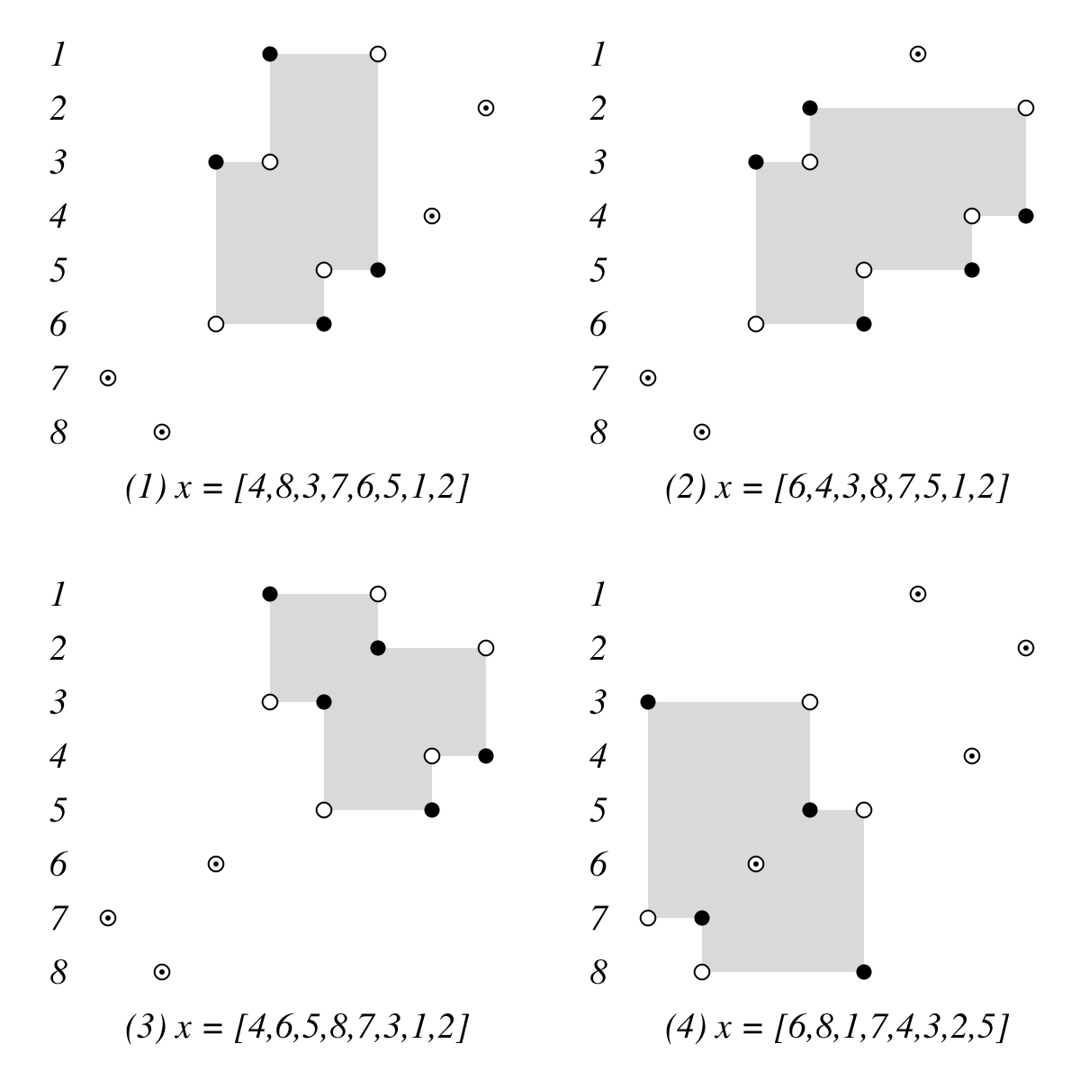
Remark 57.
The cardinality of the set may be . This is the case, for example, when
| (13.2) |
Then .
Example 58.
Using a computer it is easy to calculate, for example, that for
| (13.3) |
.
14. Patterns indexing
Which 4231 or 3412 patterns lead to elements in ? We can describe these patterns by taking all 4231 and 3412 patterns in and removing certain “useless patterns” contained in larger patterns of length 5 or 6. For example, if , the pattern 5241 will be useless since the shaded region it defines is not empty. We describe the useless patterns in the following way. For each pattern of length 5 or 6 in the left hand column of (14.1), remove the corresponding pattern in the right hand column.
| (14.1) |
The remaining “useful patterns” all index a unique component in . For example, if then has only one element namely and this element would be indexed by . This example corresponds to the shape in Figure 1.
It would be interesting to know the distribution of the various sizes of for all for large .
References
- [BB81] A. Beilinson and J. Bernstein, Localization of -modules, C. R. Acad. Sci. Paris Ser. I Math 292 (1981), 15–18.
- [Ber92] Nantel Bergeron, A Combinatorial Construction of the Schubert Polynomials, J. Comb. Theory, Series A 60 (1992), 168–182.
- [BK81] J.-L. Brylinski and M. Kashiwara, Kazhdan-Lusztig conjectures and holonomic systems, Invent. Math. 64 (1981), 387–410.
- [BL98] Sara C. Billey and Tao Kai Lam, Vexillary elements in the hyperoctahedral group, J. Alg. Combin 8 (1998), no. 2, 139–152.
- [BL00] Sara Billey and V. Lakshmibai, Singular Loci of Schubert Varieties, Progress in Mathematics, no. 182, Birkhäuser, 2000.
- [Bre94] Francesco Brenti, A combinatorial formula for Kazhdan-Lusztig polynomials, Invent. Math. 118 (1994), no. 2, 371–394.
- [Bre97] Francesco Brenti, Combinatorial expansions of Kazhdan-Lusztig polynomials, J. London Math. Soc. 55 (1997), no. 2, 448–472.
- [Bre98] Francesco Brenti, Kazhdan-Lusztig polynomials and -polynomials from a combinatorial point of view, Discrete Math 193 (1998), no. 1–3, 93–116.
- [BS98a] A. Vainshtein B. Shapiro, M. Shapiro, Kazhdan-Lusztig polynomials for certain varieties of incomplete flags, Discrete Math. 180 (1998), 345–355.
- [BS98b] Francesco Brenti and Rodica Simion, Enumerative aspects of some Kazhdan-Lusztig polynomials, Preprint (1998).
- [BW] Sara Billey and Gregory Warrington, Kazhdan-Lusztig polynomials for 321-hexagon-avoiding permutations, to appear in J. Alg. Comb.
- [Car94] J. Carrell, On the smooth points of a Schubert variety, CMS Conference proceedings, vol. 16, June 1994, pp. 15–24.
- [Che94] C. Chevalley, Sur les décompositions cellulaires des espaces , Proceedings of Symposia in Pure Mathematics 56 (1994), no. 1.
- [CK99] J. B. Carrell and J. Kuttler, On the smooth points of T-stable varieties in and the Peterson map, preprint (1999).
- [Deo85] V. Deodhar, Local Poincaré duality and non-singularity of Schubert varieties, Comm. Algebra 13 (1985), 1379–1388.
- [Dye93] M. Dyer, The nil-Hecke ring and Deodhar’s conjecture on Bruhat intervals, Invent. Math. 111 (1993).
- [Ful97] William Fulton, Young tableaux; with applications to representation theory and geometry, London Mathematical Society Student Texts, vol. 35, Cambridge University Press, New York, 1997.
- [Gas00] Vesselin Gasharov, Sufficiency of Lakshmibai-Sandhya singularity conditions for Schubert varieties, In preparation (2000).
- [Hum90] James E. Humphreys, Reflection groups and Coxeter groups, Cambridge University Press, 1990.
- [KL79] D. Kazhdan and G. Lusztig, Representations of Coxeter groups and Hecke algebras, Inv. Math. 53 (1979), 165–184.
- [Las95] Alain Lascoux, Polynomes de Kazhdan-Lusztig pour les varietes de Schubert vexillaires. (French) [Kazhdan-Lusztig polynomials for vexillary Schubert varieties], C. R. Acad. Sci. Paris Sér. I Math. 321 (1995), no. 6, 667–670.
- [LS81] Alain Lascoux and Marcel-Paul Schützenberger, Polynomes de Kazhdan & Lusztig pour les Grassmanniennes. (French) [Kazhdan-Lusztig polynomials for Grassmannians], Astérisque 87–88 (1981), 249–266, Young tableaux and Schur functions in algebra and geometry (Toruń, 1980).
- [LS84] V. Lakshmibai and C. S. Seshadri, Singular locus of a Schubert variety, Bull. Amer. Math. Soc. 11 (1984), no. 2, 363–366.
- [LS85] A. Lascoux and M.-P. Schützenberger, Schubert polynomials and the Littlewood-Richardson rule, Letters in Math. Physics 10 (1985), 111–124.
- [LS90] V. Lakshmibai and B. Sandhya, Criterion for smoothness of Schubert varieties in , Proc. Indian Acad. Sci. (Math Sci.) 100 (1990), no. 1, 45–52.
- [Man01] Laurent Manivel, Le lieu singulier des varietes de Schubert, arXiv:math.AG/0102124 (2001).
- [Pol94] P. Polo, On Zariski tangent spaces of Schubert varieties, and a proof of a conjecture of Deodhar, Indag. Math. 5 (1994), 483–493.
- [Pol99] Patrick Polo, Construction of arbitrary Kazhdan-Lusztig polynomials in symmetric groups, Represent. Theory 3 (1999), 90–104, (electronic).
- [Ste96] John Stembridge, On the fully commutative elements of Coxeter groups, J. Algebraic Combin. 5 (1996), no. 4, 353–385.
- [Zel83] A.V. Zelevinskiĭ, Small resolutions of singularities of Schubert varieties, Functional Anal. Appl. 17 (1983), no. 2, 142–144.