Diagrammatic Computations for Quandles and Cocycle Knot InvariantsThanks: The first author was supported in part by NSF Grant #9988107.Thanks: The second author was supported by Fellowships from the Japan Society for the Promotion of Science.Thanks: The third author was supported in part by NSF Grant #9988101.
Abstract.
The state-sum invariants for knots and knotted surfaces defined from quandle cocycles are described using the Kronecker product between cycles represented by colored knot diagrams and a cocycle of a finite quandle used to color the diagram. Such an interpretation is applied to evaluating the invariants.
Algebraic interpretations of quandle cocycles as deformations of extensions are also given. The proofs rely on colored knot diagrams.
Key words and phrases:
Quandles, cocycle knot invariants, knot colorings, extension cocycles.1991 Mathematics Subject Classification
Primary 57M25, 57Q45; Secondary 55N99, 18G991. Introduction
Diagrammatic morphisms interconnect algebra and topology. Complicated algebraic formulas can be established via topological diagrams, and algebraic structures give topological invariants. In this paper, we present two instances of algebraic and topological interplay from quandle homology theory. First, we use the Kronecker product and computations on colored knot diagrams for evaluating the quandle knot cocycle invariants. Second, we describe extensions of quandles by cocycles, and give diagrammatics proofs. In both examples, relations between algebra and diagrams play key roles.
A quandle is a set with a self-distributive binary operation (defined below) whose definition was motivated from knot theory. A (co)homology theory was defined in [3] for quandles, which is a modification of rack (co)homology defined in [10]. State-sum invariants using quandle cocycles as weights are defined [3] and computed for important families of classical knots and knotted surfaces [4]. Quandle homomorphisms and virtual knots are applied to this homology theory [5]. The invariants were applied to study knots, for example, in detecting non-invertible knotted surfaces [3]. On the other hand, knot diagrams colored by quandles can be used to study quandle homology groups. This view point was developed in [10, 11, 14] for rack homology and homotopy and generalized to quandle homology in [6]. It was poined out by Fenn and Rourke that the state-sum terms can be interpreted as Kronecker products. In this paper, we use such interpretations to evaluate the invariants.
The second diagrammatic method we present here is extensions of quandles. Cohomology theories of groups and other algebraic systems have interpretations in terms of group extensions or obstructions to deformations of algebraic systems (see for example [2, 13] and for a diagrammatic approach [18]). We give analogous interpretations for quandle cohomology. The proofs are based on knot diagrams.
The paper is organized as follows. In Section 1, we give a summary of preliminary material on quandle homology and cocycle knot invariants. Applications of the Kronecker product are given in Section 2, and the extensions of quandles by cocycles are investigated in Section 3.
Acknowledgement. We are grateful to Edwin Clark for his valuable comments.
2. Quandle homology and colored knot diagrams
In this section we review necessary material from the papers mentioned in the introduction.
A quandle, , is a set with a binary operation such that
(I) For any , .
(II) For any , there is a unique such that .
(III) For any , we have
A rack is a set with a binary operation that satisfies (II) and (III). Racks and quandles have been studied in, for example, [1, 8, 16, 17, 19]. The axioms for a quandle correspond respectively to the Reidemeister moves of type I, II, and III (see [8], [17], for example).
A function between quandles or racks is a homomorphism if for any .
The following are typical examples of quandles.
- •
A group with -fold conjugation as the quandle operation: .
- •
Any set with the operation for any is a quandle called the trivial quandle. The trivial quandle of elements is denoted by .
- •
Let be a positive integer. For elements , define . Then defines a quandle structure called the dihedral quandle, . This set can be identified with the set of reflections of a regular -gon with conjugation as the quandle operation.
- •
Any -module is a quandle with , , called an Alexander quandle. Furthermore for a positive integer , a mod- Alexander quandle is a quandle for a Laurent polynomial . The mod- Alexander quandle is finite if the coefficients of the highest and lowest degree terms of are .

Let be the free abelian group generated by -tuples of elements of a quandle . Define a homomorphism by
| (1) | |||||
for and for . Then is a chain complex.
Let be the subset of generated by -tuples with for some if ; otherwise let . If is a quandle, then and is a sub-complex of . Put and , where is the induced homomorphism. Henceforth, all boundary maps will be denoted by .
For an abelian group , define the chain and cochain complexes
| (2) | |||||
| (3) |
in the usual way, where , , .
The th quandle homology group and the th quandle cohomology group [3] of a quandle with coefficient group are
| (4) |
The cycle and boundary groups (resp. cocycle and coboundary groups) are denoted by and (resp. and ), so that
We will omit the coefficient group as usual if .
Let a classical knot diagram be given. The co-orientation is a family of normal vectors to the knot diagram such that the pair (orientation, co-orientation) matches the given (right-handed, or counterclockwise) orientation of the plane. At a crossing, if the pair of the co-orientation of the over-arc and that of the under-arc matches the (right-hand) orientation of the plane, then the crossing is called positive; otherwise it is negative. The crossings depicted in Fig. 1 are positive by convention.
A coloring of an oriented classical knot diagram is a function , where is a fixed quandle and is the set of over-arcs in the diagram, satisfying the condition depicted in the top of Fig. 1. In the figure, a crossing with over-arc, , has color . The under-arcs are called and from top to bottom; the normal (co-orientation) of the over-arc points from to . Then it is required that and .
Note that locally the colors do not depend on the orientation of the under-arc. The quandle element assigned to an arc by a coloring is called a color of the arc. This definition of colorings on knot diagrams has been known, see [8, 12] for example. Henceforth, all the quandles that are used to color diagrams will be finite.
In Fig. 1 bottom, the relation between the Redemeister type III move and quandle axiom (self-distributivity) is indicated. In particular, the colors of the bottom right segments before and after the move correspond to self-distributivity.
A shadow coloring (or face coloring) of a classical knot diagram is a function , where is a fixed quandle and is the set of arcs in the diagram and regions separated by the underlying immersed curve of the knot diagram, satisfying the condition depicted in the middle square of Fig. 4. In the figure, arcs are colored under the same rule as above, and the regions are also colored by the following similar rule. Let and be the regions separated by an arc colored by . Suppose that the normal to points from to . If is colored by , then is required to be colored by . Note that near a crossing there are more than one way to go from one region to another, but the self-distributivity guarantees unique colors near a crossing. In the figures, colors on the the regions are depicted as letters enclosed within squares.

Colorings and shadow colorings are defined for knotted surfaces in -space similarly using their diagrams in -space. The coloring rule is depicted in Fig. 2.


Each positive crossing in a colored knot diagram represents a pair as depicted in Fig. 1 top. The first factor is the color on an under-arc away from which the normal of the over-arc points. The color is on the over-arc. If the crossing is negative, then such colors represent . The relation between colored crossings and boundary homomorphisms is depicted in Fig. 3. The -chains represented by colored and oriented points on line segments are depicted as boundaries in Fig. 3. The color on the center vertex on an arc determine the -chain that the vertex represents. These colors are the colors at the end points of the arc in the crossing. The sign of the -chain is determined by pushing the normal to the arc into the boundary and comparing to the oriented subarc of the boundary given the counterclockwise orientation. In Fig. 3, the boundary terms of the -chain are -chains , , , and , and thier formal sum matches the negative of , where is the boundary homomorphism of quandle homology. In particular, any colored knot diagram represents a -cycle, as the boundary terms cancel.
Similarly, shadow colored crossings represent triples as depicted in Fig. 4. The boundaries are also indicated in the figure. In particular, shadow colored knot diagrams represent -cycles. The signs are determined as above and the chain (for example on the left) is determined as follows. The color is the color in the region away from which the normal to the arc colored points, and is the color on that arc.

Colored or shadow colored classical knot diagrams in orientable surfaces are defined similarly, and represent - or -cycles, respectively, as boundary terms also cancel. For example, the colored knot diagram on a surface depicted in Fig. 5 represents a -cycle in , where . In fact, , as it is known [3] that . The shaded regions in Fig. 5 are crossings of the diagram, and the unshaded crossing in the middle is a cross-over of the surface, and is not a crossing of the diagram. Since all boundaries of each colored crossing are attached to other colored crossings, we see that the boundary terms cancel, and the diagram represents a -cycle.


Furthermore, for shadow colored diagrams, we allow the colored end point diagram that is depicted in Fig. 6. Since the boundary term of the end point diagram represents , which represents zero as a quandle chain, a shadow colored knot diagram represents a quandle -cycle even with such colored end points allowed. Examples are depicted in Fig. 7 left and middle. All three diagrams in Fig. 7 represent a generator of .
These colored knot diagrams on surfaces (possibly with end points for shadow colors) are called colored abstract knot (or arc, respectively) diagrams.


Colored and shadow colored abstract knot diagrams represent cycles, and the moves for colored diagrams are known [6]: Colored diagrams related by a finite sequence of the moves represent the same homology class. Such moves are depicted in Figs. 8 and 9, and called the quandle homology moves.
The (fundamental) quandle of an -knot diagram [16, 19] is generated by the -regions of the diagram; the relations in the quandle can be read from the crossings () or double point curves (). See [8, 17] for Wirtinger presentations of knot quandles defined from knot diagrams, which are similar to Wirtinger presentations of knot groups. In this case, arcs of knot diagrams represent generators, and crossings give relations of Wirtinger form. Let represent such a quandle for a knot diagram
Let be a knot diagram on a compact oriented surface . Then the fundamental shadow quandle is defined as follows [6]. The generators correspond to over-arcs and connected components of , where the universe is the underlying immersed curves of (without crossing information). The relations are defined for each crossing as ordinary fundamental quandles, and at each arc dividing regions. Specifically, if and are generators corresponding to adjacent regions such that the normal points from the region colored to that colored , and if the arc dividing these regions is colored by , then we have the relation . This defines a presentation of a quandle, which is called the fundamental shadow quandle of . Two diagrams on that differ by Reidemeister moves on have isomorphic fundamental shadow quandles. The shadow colors are regarded as quandle homomorphisms from the fundamental shadow quandle to a quandle .
3. Cocycle invariants as Kronecker products
In this section we give an interpretation of the state-sum invariants (called quandle cocycle invariants) defined in [3] in terms of pairings on quandle homology theory. Using this interpretation, a new method of computing these invariants is given. In this section all (co)chain, (co)cycle, (co)boundary, and (co)homology groups are quandle groups and we sometimes drop the letter from the subscript or superscript.
Let be a chain complex with the boundary homomorphism . Let be the Kronecker product, where is a coefficient abelian group, and it is omitted as usual if . Thus for any and . This pairing induces a well-defined bilinear pairing (Kronecker product) .
Let be another chain complex, and denote by be the set of chain homomorphisms. For and , define
where is a fixed finite subset of . This defines a bilinear pairing . Since each Kronecker product depends only on the homology and cohomology classes, we have the following.
Lemma 3.1.
The above defined does not depend on the choice of (co)cycles and is determined only by their (co)homology classes. Thus it induces a well-defined bilinear pairing
Definition 3.2.
Let be an abstract -knot diagram, for . In the above description, let be the chain complex for a finite quandle , and be where is the fundamental quandle of a knot . A knot diagram represents a class . Pick and fix . Let be the set of all chain maps induced from all quandle homomorphisms , that is,
Define . This is called the quandle cocycle invariant of with color quandle .
A similar invariant, called shadow quandle cocycle invariant, is defined using fundamental shadow quandles , by , where and .
Remark 3.3.
The (shadow) quandle cocycle invariants coincide with the state-sum invariant defined in [3]. The set of colorings in [3] corresponds to , and the Boltzmann weight defined from a fixed cocycle corresponds to . The definition in terms of pairing was suggested to us by Fenn and Rourke in a correspondence. The above gives a generalization using quandle homology and abstract knots. The following generalizes the invariants to abstract knots.
Proposition 3.4.
The quandle cocycle invariant is an invariant for abstract knots of dimensions and (i.e., it does not depend on the choice of the diagram, and is well-defined up to equivalence of abstract knot diagrams).
The shadow quandle cocycle invariant is an invariant of knot diagrams in Euclidean spaces up to Reidemeister moves (and their analogues in dimension ).
Proof.
The equivalence relation in question does not alter the class or in the situations stated. ∎
The above interpretation can be used for computation of the invariant as follows.
Recall that is as a set with the quandle operation (mod 3). Let denote the cocycle invariant of classical knots defined by shadow colorings by and the cocycle defined by
where
In this section we give examples of this invariant using the pairing interpretations given in the previous section.
Lemma 3.5.
For any , the shadow colored diagram on the left of Fig. 7 represents a generator of .
For any , the shadow colored diagram which is the mirror image of that in the left of Fig. 7 represents the inverse of the generator of given above.
Proof.
The shadow colored diagram represents . It is known [3] that the cocycle which is defined above represents a generator of . All possibilities of are evaluated by to give the generator , and the result follows. The mirror image is checked similarly. ∎
Note that the other diagrams in Fig. 7 also represent the same generator, and have the same property as stated in the above lemma.

Proposition 3.6.
A torus knot or link is -colorable if and only if is a multiple of , for some integer . In this case, . Here is regarded as an element of .
Proof.
We represent as a closed -braid as depicted in Fig. 10. If the top two segments receive the same color, the cocycle invariant is trivial. There are such shadow colors. If the two top segments receive distinct colors, then perform the quandle homology moves as indicated in the figure, and produce a copy of a generator in Fig. 7 for each set of three crossings. By Lemma 3.5, for any choice of , the figure represents the generator of . Hence for any non-trivial coloring , . The result follows. ∎


Proposition 3.7.
A torus knot or link is -colorable if and only if is a multiple of , for some integer . If is not a multiple of , then , where is regarded as an element of . Otherwise, .
Proof.
There are three cases to color the top strings. All three colors are distinct, two colors are the same, and all colors are the same. If all colors are the same, such colorings contribute to the invariant, and there are such shadow colorings. If all colors are distinct, then such a coloring is depicted in Fig. 11 left. Such a color exists if and only if is even. Note that the color of the middle string, , stays in the middle strings. Hence we need to consider two types of shadow colors, (1) is not a color of the unbounded region, (2) it is. The case (1), (2) are shown in Fig. 11, 12 respectively. For each case, the figure shows that such a colored diagram is homologous to a copy of a generator for each set of crossings. Hence this contributes to the invariant.
By symmetry of the diagram, if two colors are the same, it can be assumed that the top strings receive, say, in this order from left to right, as depicted in the left hand side of Fig. 13. In this case must be a multiple of for such a color to exist, as can be seen from the figure. Hence the first case (when is not a multiple of ) follows from the above argument, and the cases for remain. A block of one contribution of (i.e., ) is depicted in the figure. There are such colorings, and there are such shadow colorings. There are three cases for shadow colors, as depicted in Figs. 13, 14, 15 left, respectively. For each of these cases, the figures show that they are homologous to three copies of a generator, contributing to the invariant (as each contribution is counted modulo ). The second case follows. ∎

Next we compute the invariant for doubled knots depicted in Fig. 16. These knots are twisted Whitehead doubles of the unknot. The integer represents the number of crossings as indicated. In the figure the crossings are positive ones, and if is negative, we take negative crossings.

Proposition 3.8.
A doubled knot is -colorable if and only if . If , then , and if , then .
Proof.
Figure 16 shows the first half of the statement. Note that there are trivial colorings on strings and corresponding shadow colorings, and shadow colorings corresponding to non-trivial colorings on strings. In Fig. 17, it is shown that for a particular shadow coloring, a set of three crossings in the diagrams of contributes a single copy of a generator of , and changes the crossings from positive to negative. These three negative crossings cancel with the next set of three positives. Hence this particular shadow coloring contributes from crossings. If , then the rest is a single crossing, and is a right-handed trefoil knot, giving another generator. For other choices of colorings on the regions, simply change the starting point of replacement and use the same argument. Apply type II Reidemeister moves if necessary, to reduce the given colored diagram to case. This gives the case , . If , then apply the operation in Fig. 17 times, to obtain , which is a left-handed trefoil, representing the negative of the generator. Hence the contribution is , giving . ∎

Let denote the type torus link of -components with opposite orientations given to parallel strings. In other words, is obtained from Fig. 17 with crossings by taking the “braid closure” between left and right ends.
Corollary 3.9.
The link is -colorable if and only if . In this case, .
Proof.
The method depicted in Fig. 17 applies in the same manner as in the proof of the above proposition. ∎
Remark 3.10.
The methods developed so far can be applied effectively to other examples to evaluate the invariant, directly or indirectly. As examples, we examine knots in the table. There are four knots in the table less than crossing that are -colorable: , , , and .

- •
is a generator, so if it is right-handed.
- •
is , so that .
- •
- •
is deformed to as depicted in Fig. 19, hence . The first deformation is a smoothing the second is isotopy. Compare the left bottom diagram with the second left entry of Fig. 17. The left and right half of the diagram in Fig. 19 are identified with the figure in Fig. 17, and hence can be replaced by the top left entry of Fig. 17. The result is as depicted in bottom right entry in Fig. 19.


The computational technique discussed in this section can be applied to knotted surfaces. We illustrate this with the -twist spun trefoil.
Example 3.11.
Shadow coloring is closely related to coloring a knotted surface diagram and its lower decker set. The correspondence was given in [6], but we sketch the notion briefly.
Given an embedded surface in -space, we chose a generic projection into -space and label the double points of the projection above and below to indicate their relative distance from the -space into which they are projected. The pre-image of the double point set on the surface is called the double decker set. It is separated into upper and lower pieces called the upper decker set and the lower decker set.
A quandle coloring of a knotted surface diagram induces a shadow coloring of the lower decker set considered as an abstract arc diagram in the surface. The scheme for determining this coloring is as follows: Along a double point arc, an upper sheet with color locally separates the lower sheet into two pieces (by the broken surface convention). One component of the lower sheet is colored and the other sheet is colored as depicted on the left of Fig. 2. The arc of lower decker points is colored which represents the color of the corresponding over crossing sheet. A branch point is an end-point of a lower decker arc. At such a point, the colors on the arc and surrounding -dimensional region coincide. In the lowest of the three sheets that intersect at a triple point, two lower decker arcs intersect. The arc that corresponds to the upper most sheet is depicted as un-broken on the surface, and the middle arc is broken into arcs locally. The colors on the arcs and regions match the shadow color condition depicted in Fig. 4 (see also Fig. 2).
In Figure 20, the double decker set for the -twist spun trefoil is depicted. We give a brief description on how to obtain this diagram from a movie of the -twist spun trefoil. More details can be found in [7]. The solid lines correspond to the lower decker points, and the dashed lines correspond to the upper decker points. The diagram has been colored by the -element dihedral quandle where . The integer labels on double arcs are Gauss codes. Even parity labels correspond to positive classical crossings, and odd parity labels correspond to negative crossings. Negative signs indicate undercrossings; thus all solid lines have negative labels. For example, the first type II move in a movie of the knotted surface will induce the birth of a negative and a positive crossing that are labeled and , repsectively. Immediately after the top saddle we have the Gauss code which is the standard code of the square knot. The diagram for this decker set also indicates the height with respect to the movie direction at which the critical points occur. For example the crossing in the center of the diagram that involves arcs labeled , and corresponds to the crossings between arcs labels and (on the left of the figure) and between and on the right of the figure. All three of these crossings correspond to a Reidemeister type III move among crossing points labeled , and .
In Fig. 21, only the lower decker set and colors are depicted.
We now compute the state-sum invariant of this surface by the following technique. Perform surgeries along the dotted arcs to obtain four copies of the negative of the generator given in Fig. 7. Hence this color contributes as the Kronecker product with the pull-back of the -cocycle . Hence we obtain , as we computed in [3] by a different method.
4. Extensions of quandles by cocycles
Let be a quandle and be an abelian group written multiplicatively. Let . Consider as a trivial quandle ( for any ). Let be the quandle defined on the set by the operation .
Lemma 4.1.
The above defined operation on indeed defines a quandle .
Proof.
The idempotency is obvious. For any , let be a unique element such that . Then let . Then it follows that , and the uniqueness of with this property is obvious. The self-distributivity follows from the -cocycle condition by computation, as follows.
and
We remark here that the computation above can be seen in knot diagrams in Fig. 1. Go along the string that goes from top left to bottom right in Reidemeister type III move and read off the cocycles assigned at crossings. Then it picks up the cocycles in the above two computations, for before and after the Reidemeister move, respectively. ∎
Definition 4.2.
Two surjective homomorphisms of quandles , , are called equivalent if there is a quandle isomorphism such that .
Note that there is a natural surjective homomorphism , which is the projection to the second factor.
Lemma 4.3.
If and are cohomologous, i.e., , then and are equivalent.
Proof.
There is a -cochain such that . We show that defined by gives rise to an equivalence. First we compute
which are equal since . Hence defines a quandle homomorphism. The map defined by defines the inverse of , hence is an isomorphism. The map satisfies by definition. ∎
Lemma 4.4.
If natural surjective homomorphisms (the projections to the second factor ) and are equivalent, then and are cohomologous: .
Proof.
Let be a quandle isomorphism with . Since , there is an element such that , for any . This defines a function , . The condition that is a quandle homomorphism implies that by the same computation as the preceding lemma. Hence the result follows. ∎
The lemmas imply the following theorem.
Theorem 4.5.
There is a bijection between the equivalence classes of natural surjective homomorphisms for a fixed and , and the set .
Example 4.6.
The dihedral quandle is an abelian extension of by a non-trivial cocycle. Let
where denotes the characteristic function
Let . Then an isomorphism is defined by
where denotes the largest integer not exceeding . It is checked directly that gives an isomorphism, but we can also see it as follows. The quandle operation in is characterized by the following property: if and have the same parity, then . Otherwise, , where has the same parity as but is distinct from . For an element , regard as the parity. Then by the definition of , we see that has the quandle operation with the same property as above.
Example 4.7.
The quaternion group under conjugation is a quandle. The set acts trivially on the rest as quandle operation, and the rest forms a subquandle. The obvious projection defined by is a surjective quandle homomorphism. One sees that where , , and is defined by .
Remark 4.8.
Let be a surjective quandle homomorphism, such that the equalizer has the same (finite) cardinality. Then it is an interesting problem to determine when is isomorphic to for some and .
Next we consider interpretations of -cycles in extensions of quandles. Let be a short exact sequence of abelian groups. Let be a quandle. For , let be as in the preceding section. Let be a set-theoretic (not necessarily group homomorphism) section, i.e., and .
Consider the binary operation defined by
| (5) |
We describe an obstruction to this being a quandle operation by -cocycles.
Since satisfies the -cocycle condition,
in . Hence there is a function such that
| (6) |
Lemma 4.9.
.
Proof.
First, if , or , then the above defining relation for implies that . For the -cocycle condition, one computes
and on the other hand,
so that we obtain the result. The underlines in the equalities indicates where the relation 6 is going to be applied in the next step of the calculation. ∎

Remark 4.10.
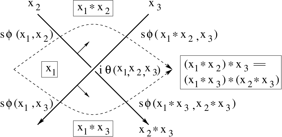
The above calculations are based on the knot diagrams as follows. In Fig. 22, two paths (denoted by dotted arcs) going from the left region to the right region are depicted in a shadow colored diagram near a crossing. Let be the top path, be the bottom path. Assign the cocycle when a dotted arc crosses an over-arc with color from the region colored to the region colored in the same direction as the normal to the over-arc. The product of these cocycles along is the left-hand side of Equality (6), and the product for appears in the right-hand side. The corresponding -cocycle is assigned to the crossing. We see this situation as follows. As we homotop to through a crossing, the descrepancy of the products is the -cocycle assigned at the crossing.
In Fig. 23, the shadow colors before/after the Reidemeister type III move is specified. The paths denoted by dotted arcs are also depicted, and named , . As we homotope the paths from to , we read off the -cocycles assigned to the crossings. The left and right of the Reidemeister move correspond to the above two computations in the proof, respectively.
Let be another section, and be a -cocycle defined similarly for by
| (7) |
Lemma 4.11.
The two -cocycles and are cohomologous, .
Proof.
Since for any , there is a function such that for any . From Equality (7) we obtain
Hence we have . ∎
Lemma 4.12.
If is a coboundary, i.e., , then admits a quandle structure such that is a quandle homomorphism.
Proof.
By assumption there is such that . Define a binary operation on by
Then by Equality (6), this defines a desired quandle operation. ∎
We summarize the above lemmas as
Theorem 4.13.
The obstruction to extending the quandle to lies in . In particular, if , then extends to for any .
Example 4.14.
For , it is known [3] that , so that there is a non-trivial extension of to defined by a generating -cocycle . It is known that , but we do not know which (if any) -cocycles obstruct extensions to with However, we obtain the following information from Theorem 4.13: for any with , the above non-trivial extension further extends to , as .
References
- [1] Brieskorn, E., Automorphic sets and singularities, Contemporary math., 78 (1988), 45–115.
- [2] Brown, K. S., Cohomology of groups. Graduate Texts in Mathematics, 87. Springer-Verlag, New York-Berlin, 1982.
- [3]
Carter, J.S.; Jelsovsky, D.; Kamada, S.; Langford, L.; Saito, M.,
Quandle cohomology and state-sum invariants
of knotted curves and surfaces,
preprint at
http://xxx.lanl.gov/abs/math.GT/9903135 .
- [4]
Carter, J.S.; Jelsovsky, D.; Kamada, S.; Saito, M.,
Computations of quandle cocycle invariants of
knotted curves and surfaces,
preprint at
http://xxx.lanl.gov/abs/math.GT/9906115 .
- [5] Carter, J.S.; Jelsovsky, D.; Kamada, S.; Saito, M., Quandle homology groups, their betti numbers, and virtual knots, to appear in J. of Pure and Applied Algebra.
- [6] Carter, J.S.; Kamada, S.; Saito, M., Geometric interpretations of quandle homology, to appear in Journal of Knot Theory and its Ramifications.
- [7] Carter, J.S.; Saito, M., Knotted surfaces and their diagrams, the American Mathematical Society, 1998.
- [8] Fenn, R.; Rourke, C., Racks and links in codimension two, Journal of Knot Theory and Its Ramifications Vol. 1 No. 4 (1992), 343-406.
- [9] Fenn, R.; Rourke, C.; Sanderson, B., Trunks and classifying spaces, Appl. Categ. Structures 3 (1995), no. 4, 321–356.
- [10]
Fenn, R.; Rourke, C.; Sanderson, B.,
James bundles and applications, preprint found at
http://www.maths.warwick.ac.uk/~bjs/ .
- [11] Flower, Jean, Cyclic Bordism and Rack Spaces, Ph.D. Dissertation, Warwick (1995).
- [12] Fox, R.H., A quick trip through knot theory, in Topology of -Manifolds, Ed. M.K. Fort Jr., Prentice-Hall (1962) 120–167.
- [13] Gerstenhaber, M.; Schack, S. D., Bialgebra cohomology, deformations, and quantum groups. Proc. Nat. Acad. Sci. U.S.A. 87 (1990), no. 1, 478–481.
- [14] Greene, M. T. Some Results in Geometric Topology and Geometry, Ph.D. Dissertation, Warwick (1997).
- [15] Inoue, A., Quandle homomorphisms of knot quandles to Alexander quandles, Preprint.
- [16] Joyce, D., A classifying invariant of knots, the knot quandle, J. Pure Appl. Alg., 23, 37–65.
- [17] Kauffman, L. H., Knots and Physics, World Scientific, Series on knots and everything, vol. 1, 1991.
- [18] Markl, M.; Stasheff, J. D. Deformation theory via deviations. J. Algebra 170 (1994), no. 1, 122–155.
- [19] Matveev, S., Distributive groupoids in knot theory, (Russian) Mat. Sb. (N.S.) 119(161) (1982), no. 1, 78–88, 160.
- [20] Roseman, D., Reidemeister-type moves for surfaces in four dimensional space, in Banach Center Publications 42 (1998) Knot theory, 347–380.
- [21]
Rourke, C., and Sanderson, B.,
There are two -twist-spun trefoils,
preprint at
http://xxx.lanl.gov/abs/math.GT/0006062 .