The Movable Fan of the Horrocks–Mumford QuinticThanks: Partially supported by the Israel Academy of Sciences and Humanities Centres of Excellence Programme, the Emmy Noether Institute for Mathematics, and the Minerva Foundation of Germany.

In this section we review the definitions and basic properties of the Horrocks–Mumford quintics. See [5], [3], and [1] for more details of these constructions.

We recall [5] that the Horrocks–Mumford bundle, $\mathcal{F}$, is a rank-$2$ vector bundle on $\mathbb{P}^{4}$, of degree $5$. A generic section of $\mathcal{F}$ vanishes on an Abelian surface, and $\Gamma(\mathcal{F})$ is $4$-dimensional.

If $s$ is a non-zero section of $\mathcal{F}$, and $p=[s]$ the corresponding point in $\mathbb{P}(\Gamma(\mathcal{F}))$, we will write $A_{p}$ for the zero locus of $s$.

The threefold $V$ is determined by the line $L$ through the two points $[s_{1}]$ and $[s_{2}]$ in $\mathbb{P}(\Gamma(\mathcal{F}))$, and is covered by the pencil of surfaces $\{\,A_{p}\mid p\in L\,\}$, giving a rational map $V\mathrel{\relbar\!\>\to}L$. We can resolve the indeterminacy of this rational map by taking

In [5, §5], it is shown that the fivefold

is non-singular. If $P_{1}$ and $P_{2}$ are two planes in $\mathbb{P}(\Gamma(\mathcal{F}))$ such that $L=P_{1}\cap P_{2}$, then $\widetilde{V}=Z\cap(\mathbb{P}^{4}\times P_{1})\cap(\mathbb{P}^{4}\times P_{2})$, and by Bertini’s theorem, this is non-singular for generic $P_{1}$ and $P_{2}$, so $\widetilde{V}$ is non-singular for generic $L$.

If $x\in V$, then the projection $\widetilde{V}\to V$ is an isomorphism at $x$ unless both $s_{1}$ and $s_{2}$ vanish at $x$, in which case $\{x\}\times L\subset\widetilde{V}$ is a rational curve contracted by the projection. Thus the singular locus of $V$ is $A_{[s_{1}]}\cap A_{[s_{2}]}$, which for generic $s_{1}$ and $s_{2}$ consists of $100$ nodes.

The centre of ${H_{5}}$ is ${\mu_{5}}$, the group of $5$th roots of $1$, and ${H_{5}}/{\mu_{5}}\cong\mathbb{Z}_{5}^{2}$. Recall from [5] that the action of $\langle{H_{5}},\iota\rangle$ on $\mathbb{P}^{4}$ preserves each surface $A_{p}$, and so preserves $V$ and can be lifted to an action on $\widetilde{V}$. Since ${\mu_{5}}$ acts trivially on $\mathbb{P}^{4}$, the $100$ nodes of $V$ form $4$ ${H_{5}}$-orbits of $25$ points, which pair up into $2$ $\langle{H_{5}},\iota\rangle$-orbits of $50$ points.

This section considers determinantal quintics, of which Horrocks–Mumford quintics are a special case.

Let $(a_{ijk})$ be complex numbers, for $i,j,k\in\mathbb{Z}_{5}$, and consider the matrix of linear forms

If $\det M(x)$ does not vanish identically, the equation $\det M(x)=0$ defines a quintic threefold $W$ in $\mathbb{P}^{4}$. Say that $M$ is nice if $W$ is regular in codimension $1$, $\rank M(x)\geq 3$ everywhere, and $\rank M(x)=4$ at all but finitely many points of $W$.

Let

The projection $\pi_{1}$ takes $X$ to $W$, with $\pi_{1}^{-1}\{x\}=\{x\}\times\mathbb{P}(\ker M(x))$, so if $M$ is nice, $\pi_{1}$ is a birational morphism, contracting finitely many rational curves on $X$.

We can construct two more matrices of linear forms from $(a_{ijk})$:

and the corresponding threefolds $W^{\prime}$, $X^{\prime}$, $W^{\prime\prime}$, and $X^{\prime\prime}$. Note that $W^{\prime}$ is the image of $X$ under the other projection $\pi_{2}$; if $M^{\prime}$ and $M^{\prime\prime}$ are also nice, we get a sequence of birational maps, all isomorphisms in codimension $1$:

Let $H$, $H^{\prime}$, and $H^{\prime\prime}$ be hyperplane sections of $W$, $W^{\prime}$, and $W^{\prime\prime}$ respectively. We can define an infinite sequence of divisors on $W$:

Solving the difference equation $D_{i-1}-4D_{i}+D_{i+1}=0$, we get

so the limits of the rays generated by $D_{i}$ as $i\to\pm\infty$ are generated by $D_{0}\pm\frac{1}{\sqrt{3}}(D_{1}-2D_{0})$; these rays then constitute the boundary of ${\overline{\mathcal{M}\mathrm{ov}}}(X)\cap{N^{1}}(X)$. (For generic $M$, $X$ is smooth, so ${N^{1}}(X)={\widetilde{N}^{1}}(X)$ and these rays are the boundary of ${\overline{\mathcal{M}\mathrm{ov}}}(X)$.)

Now let $y\in\mathbb{C}^{5}$, and consider the matrix $M_{y}$, where

and the corresponding varieties and maps

Because $M_{y}^{\scriptscriptstyle T}=M_{\iota y}$, this sequence can also be written as

From [3, attributed there to R. Moore] we see that, if $V$ is a sufficiently general HM quintic, and $y$ is any node of $V$, then $V=W_{y}$; also that there is an automorphism of the space of HM quintics, $\beta$, such that $\beta V=W^{\prime}_{y}$.

Therefore, (3) and (4) can also be written as

From now on all threefolds we consider will be isomorphic in codimension $1$ to a fixed sufficiently general HM quintic $V$. We can therefore identify corresponding divisors in any two of these threefolds. Any such divisor determines a point in the real vector space $N={\widetilde{N}^{1}}(V)={N^{1}}(\widetilde{V})$.

Choose representatives $y_{1},\ldots,y_{4}$ (respectively, $z_{1},\ldots,z_{4}$) of the four ${H_{5}}$-orbits of nodes of $V$ (respectively, of $\beta^{-1}V$), such that $\iota y_{1}=y_{3}$, $\iota y_{2}=y_{4}$, $\iota z_{1}=z_{3}$, and $\iota z_{2}=z_{4}$. Then $V$ fits into six different sequences of the form (5):

This gives us $12$ divisors on $V$:

• $\Delta_{i}$, the strict transform under $\phi_{y_{i}}$ of a hyperplane section of $\beta V$.

• $\nabla_{i}$, the strict transform under $\phi^{\prime\prime}_{\iota z_{i}}$ of a hyperplane section of $\beta^{-1}V$.

• $\nabla^{\prime}_{i}$, the strict transform under $\phi_{z_{i}}$ of a hyperplane section of $V$.

We also have $H$, a hyperplane section of $V$, and $A$, one of the pencil of Abelian surfaces on $V$. By Lemma 1, we have $\Delta_{i}+\iota\Delta_{i}\sim\nabla_{i}+\nabla^{\prime}_{i}\sim 4H$.

We write $\Lambda_{i}$ for the rational curve on $\widetilde{V}$ that is contracted to the node $y_{i}$ on $V$. Noting from [2] that a singular member of the pencil of surfaces $\{A_{p}\}$ is an elliptic scroll, we let $\Gamma$ be a line in one of these scrolls.

The following intersection numbers on $\widetilde{V}$ are computed in [3] ($\Lambda_{1},\Lambda_{2},\Lambda_{3},\Lambda_{4}$ are there called $L_{1},L_{3},L_{2},L_{4}$—note the different order):

We can now draw a picture of a neighbourhood of the ray generated by $H$ in $N$ (Figure 1), showing the structure of the movable fan there: taking the affine slice of the fan given by $(\Gamma+\Lambda_{1}+\Lambda_{3})\cdot D=2$, we find that the four planes given by $\Lambda_{i}$ divide the neigbourhood up in such a way that the vertex figure is a cuboctohedron (as do any four planes in general position through a point). The $12$ vertices of this cuboctohedron are on the lines joining $2H$ to the $12$ divisors constructed out of the determinantal description ($\Delta$s and $\nabla$s) (see Figure 2).

Let $\nabla$ be any of these $12$ divisors. Coming as it does from pulling back an ample divisor on a model of $V$ with Picard number $1$, it generates a $1$-dimensional cone—a ray—in the movable fan. (2) in section 2 shows that there is a marked model, not necessarily minimal, of $V$, that is simultaneously a partial small resolution of the two marked models corresponding to $H$ and $\nabla$, so there is a cone in the fan whose closure contains both rays.

Therefore the $12$ rays generated by the $\Delta$s and $\nabla$s are neighbours in the fan to the ray generated by $H$, and the cuboctohedral arrangement extends as far as these neighbouring rays (Figure 2). Since the marked models corresponding to these rays are all isomorphic, ignoring the marking, either to $V$ or to $\beta V$, there will be a similar cuboctohedral figure about each of them, and so about every ray of the fan that can be reached from $H$ along $2$-dimensional cones of the fan.

In the next two sections we will describe the nef cones of the resolutions of $V$—that is, the $4$-dimensional cones of the fan whose closure contains $H$. This will lead to a complete description of the movable fan. These nef cones are the duals to the cones of curves described in [3], but our notation and point of view are different, and we need several details not found there.

Whenever we refer to the cuboctohedral neighbourhood of a ray in the fan, we will use terms such as top and left, assuming that the cuboctohedron is oriented as in Figures 1 and 2.

The nef cone of $\widetilde{V}$ lies in the sector of the cuboctohedral figure given by the conditions $\Lambda_{i}\cdot D\geq 0$; it contains the square face of the cuboctohedron spanned by $\nabla^{\prime}_{1}$, $\nabla^{\prime}_{2}$, $\nabla^{\prime}_{3}$, and $\nabla^{\prime}_{4}$—that is, the bottom square face in the diagram.

In [3, p. 31] it is shown that $\phi^{\prime}_{z_{i}}$ (there called $\phi_{\nabla^{\prime}_{i}}$) lifts to a biregular automorphism of $\widetilde{V}$, acting by translation on each Abelian surface $A_{p}$, and that $\phi^{\prime}_{z_{1}}$ and $\phi^{\prime}_{z_{2}}$ generate a free abelian group of rank $2$; in terms of the basis (7), this group acts as the group of matrices

Now we have enough information to describe the nef cone of $\widetilde{V}$.

Since $\Aut\widetilde{V}$ acts transitively on the faces of ${\,\overline{\!\mathcal{A}\mathrm{mp}}}(\widetilde{V})$, all models of $V$ that can be obtained by making one flop from $\widetilde{V}$ are isomorphic. So let us consider the variety $\widetilde{V}_{1}$ obtained by flopping in the $\Lambda_{1}$ face, so that $-\Lambda_{1}$ is effective on $\widetilde{V}_{1}$.

The nef cone can be found easily in this case:

The apex of the pyramid, $\Delta_{1}$, gives a contraction to $\beta V$, and also has a cuboctohedral neighbourhood. We can see that the cone just described must fit into the top square face of this cuboctohedron, since the bottom face is occupied by a model $\cong\beta\widetilde{V}$, and the top face is the only other face fixed by an automorphism of the movable fan of order $2$.

Although there are two $\Aut\widetilde{V}_{1}$-orbits of triangular faces of this pyramid, the whole situation is symmetric (the two are swapped by changing our arbitrary choice of $y_{1}$ and $y_{2}$ at the beginning of section 3), so we only need to analyse one of the flops. Let us consider $\widetilde{V}_{2}$, obtained by flopping $\widetilde{V}$ in the planes defined by $\Lambda_{1}$ and $\Lambda_{2}$.

Since this involves the upper triangular faces of the cuboctohedron, it completes the job of describing cones that meet $H$—that is, nef cones of resolutions of $V$. But now every face of any of these cones borders another cone of one of these three types, so we have in fact described every cone in the fan:

From the theorems of the last two sections we can deduce a complete combinatorial description of the movable fan of $V$, since they give the shapes of the cones and the way the cones fit together at each ray. In this section we aim to give an understanding of the combinatorics of the movable fan as a polyhedral complex, disregarding the linear structure, and of the action on that complex of the birational automorphism group. So we will allow ourselves to squash and fold the cones. We will talk in terms of affine slices, making it a problem about $3$-dimensional solids.

The first thing we can do to simplify matters is to glue the pyramids to the faces of the tilings. The result is a solid, no longer convex, with twice the vertices of the old square tiling, arranged like a square tiling again (at $45^{\circ}$ to the old one), but with half the vertices protruding and with a diagonal inward fold (marked by dotted lines in Figure 6) across each face.

This reduces the problem to two sorts of solid, these stellated tilings and the lozengoids. Now the lozengoid of Figure 5 can be regarded as a cube distorted in such a way that two opposite faces (the top and bottom faces in Figure 5) become folded outwards along their diagonals (see Figure 7).

The way these cones are put together sets the dotted ridges on the lozengoids into the dotted furrows on the tilings, so we can flatten these folds to obtain a complex of ordinary cubes and square-tiled paraboloids.

Consider what has happened to the vertex figure (Figure 2) in this process: gluing the pyramids to the tilings has the effect of deleting the four edges around the bottom face of the cuboctohedron, leaving four downward-pointing spikes, which are flattened out when the dotted edges on the solids are flattened. The result is a square antiprism (Figure 8). A square tiling pokes into the each of the two square faces and a cube pokes into each triangular face.

It is easily seen that this vertex configuration determines a unique simply connected polyhedral complex, because there is no choice about how the figures at two adjacent vertices are oriented with respect to one another. But we can construct such a simply-connected polyhedral complex with this configuration at every vertex as a uniform hyperbolic tiling (see [4], [6]) as follows:

The Coxeter graph $\circ\!\!=\!\!\circ\!\!=\!\!\circ\!\!=\!\!\circ$ describes a hyperbolic reflection group $C$ with a tetrahedral fundamental cell: the nodes of the graph correspond to the faces of the cell, and the angle between two faces is $\pi/8$ if the two nodes are joined by a double line, and $\pi/4$ if the two nodes are not joined. The marked graph $\bullet\!\!=\!\!\circ\!\!=\!\!\circ\!\!=\!\!\bullet$ represents a hyperbolic tiling with $C$ acting transitively on its vertices: the unique vertex of the tiling that is in the fundamental cell lies on the faces of the cell corresponding to unfilled nodes in the marked graph, and not on the faces corresponding to filled nodes. $C$-orbits of $k$-dimensional faces of the tiling are described by $k$-node subgraphs of $\bullet\!\!=\!\!\circ\!\!=\!\!\circ\!\!=\!\!\bullet$ having at least one marked node in each connected component (for example, deleting an end node gives $\bullet\!\!=\!\!\circ\!\!=\!\!\circ$, a square tiling, and deleting a middle node gives $\bullet\!\!=\!\!\circ\quad\bullet$, a square prism), so it is possible to work out the vertex configuration of this tiling: it is the same square antiprism as produced above.

Therefore we can identify the birational automorphism group of $V$:

The aim of this section is to demonstrate that, although by the results of the last section the movable fan of $V$ is combinatorially similar to a tiling of hyperbolic $3$-space, the cone ${\mathcal{M}\mathrm{ov}\!_{\scriptscriptstyle+}}(V)$ itself is more subtle, by proving this theorem:

The description of the nef cones in sections 4 and 5 allows us to find all the effective divisors on the boundary of the movable cone, since every such divisor is nef on some model. But the only rays in any of the nef cones described above that are in the boundary of ${\mathcal{M}\mathrm{ov}\!_{\scriptscriptstyle+}}(V)$ are those corresponding to Abelian fibrations on tiling type models. These rays must then be dense on the boundary, and we can investigate the shape of the boundary through them. So let us see how we can produce examples of these points.

From $\widetilde{V}$ we can flop the four classes of curves $\Lambda_{1},\ldots,\Lambda_{4}$ to get a pyramid type model (the top of the cuboctohedron), from which we can flop one more class, say $\Lambda^{\prime}$, to get a model $\widetilde{V}^{\prime}\cong\beta\widetilde{V}$. We know that $\Lambda^{\prime}\cdot\nabla_{i}=0$ for $i=1,\ldots,2$, and $\Lambda^{\prime}\cdot H=1$, which determine $\Lambda^{\prime}$; it can easily be checked that $\Lambda^{\prime}=3(\Lambda_{1}+\Lambda_{3})+\Gamma$.

Let $A^{\prime}$ be the class of an Abelian fibre on $\widetilde{V}^{\prime}$, and $\Gamma^{\prime}$ be the class of a line in a singular fibre of the Abelian fibration given by $A^{\prime}$. Recall that in Corollary 5 we defined an $\Aut\widetilde{V}$-invariant quadratic form $Q$ by $Q(D,E)=d_{1}e_{4}+d_{4}e_{1}-2d_{2}e_{2}-2d_{3}e_{3}$, in the basis (7). Let $Q^{\prime}$ be the $\Aut\widetilde{V}^{\prime}$-invariant quadratic form defined in the same way with reference to $\widetilde{V}^{\prime}$.

To get from $\widetilde{V}$ to this model we have the flopped the curves in each of the five classes $\Lambda_{1},\ldots,\Lambda_{4}$, and $\Lambda^{\prime}$, so we know $A^{\prime}\cdot\Lambda_{1}=\cdots=A^{\prime}\cdot\Lambda_{4}=A^{\prime}\cdot\Lambda^{\prime}=-1$, which determines $A^{\prime}$ exactly:

We can also do this process in reverse, flopping a face of ${\,\overline{\!\mathcal{A}\mathrm{mp}}}(\widetilde{V})$, say that given by $L_{1}$, and four more faces to get a model $\widetilde{V}^{\prime\prime}\cong\beta\widetilde{V}$. Then $\widetilde{V}$ bears the relation to $\widetilde{V}^{\prime\prime}$ that $\widetilde{V}^{\prime}$ bears to $\widetilde{V}$, so $A=5\Delta_{1}-A^{\prime\prime}$; that is,

Therefore we have

so

This is enough to prove Theorem 10:

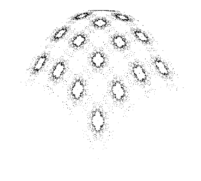
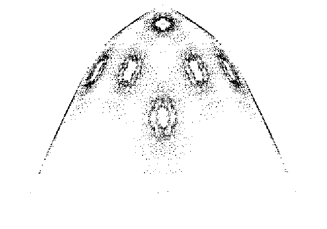
The two processes for obtaining new boundary rays from old can be iterated; the plots in Figure 10 are of two different orthogonal projections of and affine slice of some such rays, showing the subtle shape of the boundary.

Finally, we can check explicitly that $V$ satisfies Morrison’s movable cone conjecture [8]:

References

- [1] A. B. Aure, Surfaces on quintic threefolds associated to the Horrocks–Mumford bundle, Arithmetic of Complex Manifolds, Lecture Notes in Math., no. 1399, Springer-Verlag, 1989, pp. 1–9.
- [2] W. Barth, K. Hulek, and R. Moore, Degenerations of Horrocks–Mumford surfaces, Math. Ann. 277 (1987), 735–755.
- [3] C. Borcea, On desingularized Horrocks–Mumford quintics, J. Reine Angew. Math. 421 (1991), 23–41.
- [4] H. S. M. Coxeter, Regular polytopes, third ed., Dover, 1973.
- [5] G. Horrocks and D. Mumford, A rank 2 vector bundle on with 15,000 symmetries, Topology 12 (1973), 63–81.
- [6] J. Humphreys, Reflection groups and Coxeter graphs, Cambridge Studies in Advanced Mathematics, no. 29, Cambridge University Press, 1990.
- [7] Y. Kawamata, Crepant blowing-up of 3-dimensional canonical singularities and its application to degenerations of surfaces, Ann. of Math. 127 (1988), 93–163.
- [8] D. Morrison, Beyond the Kähler cone, Proceedings of the Hirzebruch 65 Conference, Bar-Ilan Univ., 1966, pp. 361–376. alg-geom/9407007.
- [9] by same author, Compactifications of moduli spaces inspired by mirror symmetry, Journées de Géométrie Algébrique d’Orsay 1992, Astérisque, no. 218, 1993, pp. 243–271. alg-geom/9304007.
Institut für Mathematik, Universität Hannover,
Postfach 6009, D 30060 Hannover, Germany