Holistic projection of initial conditions onto a finite difference approximation
Abstract
Modern dynamical systems theory has previously had little to say about finite difference and finite element approximations of partial differential equations (pdes) [1]. However, recently I have shown one way that centre manifold theory may be used to create and support the spatial discretisation of pdes such as Burgers’ equation [2] and the Kuramoto-Sivashinsky equation [3]. In this paper the geometric view of a centre manifold is used to provide correct initial conditions for numerical discretisations [4]. The derived projection of initial conditions follows from the physical processes expressed in the pdes and so is appropriately conservative. This rational approach increases the accuracy of forecasts made with finite difference models.
PACS:
02.60.Lj, 02.70.Bf, 05.45.-a
Keywords:
Burgers’ equation, initial condition, holistic finite differences.
1 Introduction
Consider the equations for some physical field evolving in space-time that we wish to model numerically. Imagine a given initial field and a finite difference model written in terms of for equi-spaced grid points say; for example, in §2 for Burgers’ equation (3) we find
| (1) |
in terms of the central difference operator and central mean operator . One might expect that the correct initial condition for this discretisation is simply to project the initial field onto the finite dimensional space of the model by setting the initial discretisation values to the value of the initial field at the grid: . But if the initial field is localised away from any grid point then physically we know to distribute the initial field among nearby grid points. I use dynamical arguments to show that the correct initial condition is, to leading order, the correctly conservative element average
| (2) |
This formula, and higher order corrections that involve neighbouring elements, are derived systematically herein. For a numerical model, this is the first time a dynamical rationale has been used to provide initial conditions.
Such projection of initial fields onto the discretisation is supported by centre manifold theory [5, e.g.]: the Relevance Theorem asserts that each of the nearby solutions of the governing pde exponentially quickly in time approach a solution of the numerical model; this holds even for finite grid spacing . The algebraic techniques developed by Roberts [4], based upon analysing with the aid of computer algebra the adjoint of a linearisation of the pde, determines the initial condition for the discretisation so that we ensure the finite difference model faithfully tracks the correct particular solution of the pde.
2 Burgers’ equation is discretised with centre manifold theory
Consider the dynamics of Burgers’ equation
| (3) |
as a prototype advection-diffusion equation. Roberts [2] first constructed finite difference approximations to the spatial derivatives using centre manifold theory to ensure nonlinear, subgrid-scale processes were systematically modelled. We summarise the approach in this section.
Divide the spatial domain into a number, say , of elements of equi-size . We analyse the dynamics of the elements away from any physical boundary to derive a discretisation for the interior of the domain. Artificially crafted internal boundary conditions (ibc’s) between the elements are introduced:
| (4) |
where denote the jump across each internal boundary, denotes the average value from the two sides of the boundary, and distinct from earlier work [2] these ibc’s are expressed in terms of the flux . See that when the right-hand side of the second ibc disappears so that the two conditions then completely insulate an element from its neighbours. Whereas when , the left-hand side disappears and the two conditions ensure sufficient continuity of the physical field to recover Burgers’ dynamics throughout the domain.
The centre manifold and the evolution thereon is straightforwardly constructed using the computer algebra algorithm described in [2, 6]. Here we find the subgrid field in the th element is
| (5) |
where ranges over . The evolution on this centre manifold, when evaluated at to restore continuity, forms the finite difference model (1) for Burgers’ equation: see that the first three terms in (1) form a standard discretisation of each term but now appearing automatically from the discretisation when mediated by the flux form (4) of the ibc’s; whereas the last term gives corrections to account for interactions between the nonlinear advection and the diffusive dissipation. Such nonlinear modifications of standard discretisations can be extremely effective [2].
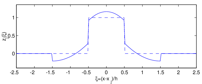
To find the correct initial condition, , for numerical models such as (1) corresponding to any given field , we follow the procedure described in [4]. The aim is to determine projection vectors , such as those shown in Figure 1, so that
| (6) |
as the inner product.
Now the dynamics linearised about the nonlinear centre manifold, , is governed by the operator
with ibc’s linearised about (4) of
| (7) |
Then in the above inner product the adjoint of is
| (8) |
To find the projection vectors we start with the leading approximation corresponding to (2) and plotted in Figure 1, where denotes the characteristic function that is in the th element and otherwise is . Then successive corrections are sought by iteration to ultimately satisfy the appropriate version of the equations derived in [4]: defining the dual operator we must solve
| (9) |
subject to the ibc’s in (8) and the normalisation condition
| (10) |
where is the tangent vector of the centre manifold. We seek solutions in a power series in to errors corresponding to the finite difference approximation of stencil width . A computer algebra program available from the author does all the necessary algebra.
3 Project onto Burgers’ discretisation
In this section we solve to quantities with errors : the finite difference model for Burgers’ equation is then (1); and the corresponding centre manifold over the whole domain is given by (5). Calculating to errors the projection onto the numerical model must be orthogonal to
| (11) | |||||
Higher order expressions may be straightforwardly computed by computer algebra. I conclude by further interpreting the physical effects incorporated in the projection defined by the above .
3.1 Linear diffusion
Set in this subsection to analyse the linear diffusion equation . Then the projection vector (11), evaluated at to recover the physically relevant case as plotted in Figure 1, is
| (12) |
To find the correct initial condition using this in (6) note that in these linear diffusion dynamics by the normalisation (10); thus here . For example, see that a point release in the th element, , requires the slightly distributed initial condition
| (13) |
Such a specific initial condition corresponds via (5) to a field on the centre manifold as shown in Figure 2 for the three cases , and .
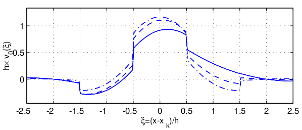
See that these initial conditions ensure that the first moment of the numerical solution is correct for all time: in the numerical model (1) the first moment is constant in time so it is enough to check that the first moment is correct in the initial conditions. Define , then for all time both in the model and in the exact solutions. The first moment in the exact solution is its initial value ; from (13) the first moment in the numerical model is the same
However, the second moment has errors: it evolves in time at the correct rate , but the initial value is instead of . Determining the projection of initial conditions to higher orders in the coupling parameter obtains such higher order moments correctly. Note that the rational approach adopted here does better than the usually chosen initial conditions which incur errors.
3.2 Nonlinear dynamics
Consider the terms from (11) that modify (12), namely
Realise that the leading order effect of including these terms is to modify the initial condition by . For example, if the initial field is approximately constant, , then
that the coefficients of the characteristic functions sum to zero reflects that the the projection conserves the field . More specifically, if is except for a symmetric bump in the th element, then as well as the direct symmetric distribution identified for linear diffusion, the component in causes to increase and to decrease by an amount proportional to reflecting that the self advection of the bump is not as great as that induced by assigning the mass of the bump solely to . Conversely, for an antisymmetric perturbation in the th element, positive to the left of , the component in increases and decreases in proportion to to reflect the increased delay in advecting out of the th element because more of it is further to the left initially. The terms in (11) reflect more subtle physical processes.
4 Conclusion
Based upon the method of analysis and the discussion in the previous sections, we deduce that this centre manifold approach to finding correct initial conditions for finite difference models accounts for subgrid scale processes that occur as initial transients decay. No other method does this.
Extensions of this approach to higher spatial dimensions is straightforward. For example, consider the class of diffusive pde’s
where represents nonlinear reaction or advection effects. After tessellating space into finite elements—using ibc’s of the form (cf (4))
where is the flux of normal to the internal boundary and is a size of the element—the fundamental problem in constructing a model is simply to solve Poisson’s equation with forced Neumann boundary conditions on each element. The adjoint of this problem lies at the heart of the dual (9) for determining initial conditions of the approximation. Although these sub-grid problem may itself need to be done numerically, in the simplest case of a regular tessellation it need only be done once for each term in the model, just like the computation of the interaction terms in a traditional finite element approximation.
In the case where there are variations in the size or shape of the elements of the discretisation, one would build formulae for the approximation parametrised by the shapes of the element and those neighbouring elements to which it is coupled by the ibc’s. The algebraic detail becomes more complicated but the principles are the same.
References
- [1] B. García-Archilla and E. S. Titi. Postprocessing the Galerkin method: the finite element case. SIAM J. Num. Anal., 37:470–499, 2000.
- [2] A. J. Roberts. Holistic discretisation ensures fidelity to Burgers’ equation. Applied Numerical Modelling, 2000. to appear.
- [3] T. Mackenzie and A. J. Roberts. Holistic finite differences accurately model the dynamics of the Kuramoto-Sivashinsky equation. ANZIAM J., 42(E):C918–C935, 2000. [Online] http://anziamj.austms.org.au/V42/CTAC99/Mack.
- [4] A. J. Roberts. Computer algebra derives correct initial conditions for low-dimensional dynamical models. Comput. Phys. Comm., 126(3):187–206, 2000.
- [5] J. Carr. Applications of centre manifold theory, volume 35 of Applied Math. Sci. Springer-Verlag, 1981.
- [6] A. J. Roberts. Low-dimensional modelling of dynamics via computer algebra. Comput. Phys. Comm., 100:215–230, 1997.