Tilings of quadriculated annuli

A quadriculated surface ^†† 1991 Mathematics Subject Classification. Primary 05B45, Secondary 05A15, 05C50, 05E05. Keywords and phrases Quadriculated surfaces, tilings by dominoes, dimers.^†† The authors gratefully acknowledge the support of CNPq, Faperj and Finep (Brazil). The authors thank the referee for the many suggestions which have improved the presentation. is a juxtaposition of squares along sides forming a surface (usually with boundary) such that vertices of squares which lie in the interior of the surface belong to precisely four squares and vertices in the boundary belong to finitely many squares. A simple example of a quadriculated surface is the quadriculated plane, ${\mathbb{R}}^{2}$ divided into unit squares with vertices in ${\mathbb{Z}}^{2}$. Compact quadriculated surfaces have finitely many squares and will usually be bicolored and balanced, i.e., the forming squares are black and white in such a way that squares with a common side have opposite colors, and the number of black squares equals the number of white squares.

Let $A$ be a balanced quadriculated annulus: $A$ is topologically ${\mathbb{S}}^{1}\times[0,1]$ and can be embedded in ${\mathbb{R}}^{2}$. We assume $A$ to be a subset of the plane, allowing free use of an orientation of $A$ and of its inner and outer boundaries.

Let $T_{A}$ be the set of domino tilings of $A$. For $t\in T_{A}$, we draw inside each domino a domino arrow from the center of the black square to the center of the white square. Given $t_{0},t_{1}\in T_{A}$, juxtapose the domino arrows from $t_{1}$ to the reversed domino arrows from $t_{0}$: this produces a finite number of oriented simple closed curves. The flux $\phi(t_{1};t_{0})$ of $t_{1}$ relative to $t_{0}$ counts such curves with weights $-1$, 0 or 1 given by the winding of each curve in the annulus $A$. The word flux has been chosen for its (co)homological connotations; unfortunately, this use of the term is unrelated to that of Lieb and Loss ([7]). The flux polynomial of $A$ is

this is a Laurent polynomial in $p$ which is independent of base tiling $t_{0}$, up to multiplication by an integer power of $p$.

When the roots of $\Phi_{A}^{+}(p)$ are distinct, $-1$ may or may not be a root.

A tiling $t$ induces a bijection $\beta_{t}$ from black to white squares. Again fixing an arbitrary base tiling $t_{0}\in T_{A}$, let the sign $\sigma(t;t_{0})$ of a tiling $t$ relative to $t_{0}$ be the sign of the permutation $\beta_{t}\circ\beta_{t_{0}}^{-1}$ on the set of white squares. Deift and Tomei ([1]) pointed out that $-1$-counting of tilings on disks can only yield very few values.

The signed flux polynomial of an annulus $A$ is

an expression independent of base tiling up to sign and multiplication by a power of $p$. On quadriculated annuli, $-1$-counting is also severely restricted.

Actually, we study a more general polynomial, the $q$-flux polynomial of $A$,

which enumerates tilings of $A$ according to volume $\nu$ and flux. Counting according to volume (defined in Section 4), i.e., $q$-counting of domino tilings, has been considered previously: in [2], for example, Elkies, Kuperberg, Larsen and Propp $q$-count tilings by dominoes of the Aztec diamond and MacMahon ([8]) already $q$-counted lozenge tilings. The flux polynomials are special cases of the $q$-flux polynomial: $\Phi_{A}^{+}(p)=\Phi_{A}(p,1)$ and $\Phi_{A}^{-}(p)=\Phi_{A}(p,-1)$.

The main ingredient in the proofs is the fact that $\Phi_{A}(p,q)$ has two distinct algebraic interpretations. The first one is rather familiar: $\Phi_{A}(p,q)$ is the determinant of a Kasteleyn-type matrix $M_{A}(p,q)$ (see Section 4). The second interpretation requires the construction of another matrix: for each flux $f$, the coefficient of $p^{f}$ in $\Phi_{A}(p,q)$ (a Laurent polynomial in $q$) is the trace of a connection matrix obtained as follows (see Section 6). Tear $A$ along a cut formed by sides of squares (as in Figure 1) giving rise to a periodic track segment: a (topological) quadriculated rectangle $\Delta$ with a marked pair of opposite sides, the left and right attachments (see Figures 9 and 10). Now, a tiling of $A$ almost induces a tiling on $\Delta$: the complication is that the dominoes of the tiling, when drawn so as to fill $\Delta$ completely, may trespass the attachments. Our definition of tiling of a track segment shall allow dominoes to trespass attachments (again as in Figure 9). We list, for a given value of the flux $f$, all possible ways in which dominoes can trespass the attachment (the indices of an attachment). Say there are $N$ such ways: the $N\times N$ connection matrix $C_{\Delta,f}(q)$ has for $(i,j)$-entry the $q$-counting of tilings of $\Delta$ trespassing left and right attachments in the way prescribed by indices $i$ and $j$. Rather unsurprisingly, the connection matrix depends in an irrelevant fashion on the choice of cut.

Both Kasteleyn and connection matrices are well behaved with respect to taking the quadriculated $n$-cover $A^{n}$ of an annulus $A$. As we shall see in Section 5, the Kasteleyn matrix associated to $A^{n}$ has for determinant a polynomial $\Phi_{A^{n}}(p,q)$ whose roots, for fixed $q$, are, up to sign, the $n$-th power of the roots of $\Phi_{A}(p,q)$ for the same fixed $q$. Thus, we may study the roots of $\Phi_{A}(p,q)$ by considering different $n$-covers of $A$. For connection matrices, the relationship is even simpler: $C_{\Delta^{n},f}=(C_{\Delta,f})^{n}$ (Section 6). Here, $\Delta$ is a periodic track segment obtained from $A$ by a cut and $\Delta^{n}$ is the juxtaposition of $n$ copies of $\Delta$, i.e., the periodic track segment obtained by cutting $A^{n}$.

The connection matrix $C_{\Delta^{n},f}$ has two useful features. First, the computation of each entry is a counting of tilings on a disk: indeed, the indices associated to left and right attachments, obtained by the row and column of an entry, indicate how to prune $\Delta$ at the attachments yielding a disk $D$ so that tilings of $\Delta$ with prescribed indices are tilings of the disk $D$, which are then $q$-counted. We may then apply Theorem 1.2 to infer that, in the case of $(-1)$-counting, connection matrices can have very few values for their entries. By finiteness, there must be different integers $n_{0}$ and $n_{1}$ for which, for all possible values of the flux $f$, we must have $(C_{\Delta,f}(-1))^{n_{0}}=(C_{\Delta,f}(-1))^{n_{1}}$ and hence $\Phi_{A^{n_{0}}}(p,-1)=\Phi_{A^{n_{1}}}(p,-1)$. Since the roots of $\Phi_{A^{n}}(p,-1)$ are, up to sign, $n$-th powers of the roots of $\Phi_{A}(p,-1)$, this essentially proves that the non-zero roots of $\Phi_{A}(p,-1)$ are roots of unity—this is Theorem 1.3. The second feature of the connection matrix is the simple fact that, by definition, it has only non-negative entries when $q>0$. This permits the study of its eigenvalues (and thus, its trace) by making use of the Perron theorem for non-negative matrices.

In Section 2, we introduce wall-free annuli, essentially irreducible quadriculated annuli with respect to the set of tilings. For annuli admitting walls, the theorems have more stringent statements, with simple proofs. In this section, we introduce most of the notation used in the paper and a convenient discrete version of the Gauss-Bonnet theorem.

In Section 3, we review the basic facts about height functions, algebraic descriptions of tilings of a simply connected quadriculated region ([10]). Tilings of an annulus $A$ give rise to periodic tilings on $A^{\infty}$, which are then studied as height functions in the band $A^{\infty}$.

In Section 4, we define Kasteleyn weights on $A$. This is a modification of Kasteleyn’s construction ([4], [5]). In more detail, cut $A$ to obtain a periodic track segment $\Delta$ and a Kasteleyn triple of matrices: one accounting for interaction between black and white squares whose common side is not in the cut, and two others which account for interaction of squares across the cut. The triple is convenient when studying the effect of juxtaposition and closing of track segments. The $q$-flux polynomial $\Phi_{A}(p,q)$ is the determinant of a matrix obtained in a simple fashion from the Kasteleyn triple. We build up from three simple homomorphisms—flux, volume and sign—on the (additive) group of 1-cycles on $A$. The homomorphisms have simple combinatorial interpretations and incorporate well the properties required for obtaining $(p,q)$-counting of tilings out of a determinant. In Section 5, we show how Kasteleyn triples and the $q$-flux polynomial behave with respect to $n$-covers of the annulus $A$.

Section 6 describes the connection matrix $C_{\Delta,f}$. The proof of Theorem 1.3 ends the section. Most of Section 7 is dedicated to the positivity of certain matrix entries which is needed to use Perron’s theorem. We finally prove the following generalization of Theorem 1.1.

There is a natural symbolic dynamical context for the results in this paper which shall not be explored in detail (see [6] for terminology and basic results). For the band $A^{\infty}$, let $T_{A^{\infty},f}$ be the set of tilings of $A^{\infty}$ with flux $f$; $T_{A^{\infty},f}$ is a Cantor set under a natural sequence space topology. Translation of tilings by one period corresponds to the shift in sequence space and is a homeomorphism from $T_{A^{\infty},f}$ to itself. With this structure, $T_{A^{\infty},f}$ is a topological Markov chain with transitive matrix and therefore topologically mixing and with a dense set of periodic tilings. Furthermore, translation preserves a certain class of measures constructed taking into account the combinatorics of tilings.

It seems natural to ask if similar results can be obtained for tilings by lozenges of triangulated annuli (a lozenge is a juxtaposition of two equilateral triangles along a common side of length 1). We indicate two significant difficulties. First, there is no obvious counterpart to Theorem 1.2. Besides, the technical requirements to prove eventual compatibility, indeed, the very concept of wall, have not, to our knowledge, been sufficiently studied. Another related problem is the study of other surfaces such as tori and surfaces of higher genus with boundary. This must involve polynomials in more variables to account for the value of the flux across independent cuts.

In the introduction we already presented the concepts of bicolored and balanced quadriculated surfaces. We always consider disks and annuli embedded in ${\mathbb{R}}^{2}$ but not necessarily in the quadriculated plane. Let $T_{S}$ be the set of domino tilings of a quadriculated surface $S$. A path $v_{0}v_{1}\ldots v_{n}$ in $S$ is a sequence of adjacent vertices. A path $v_{0}\ldots v_{n}$ turns left (resp. right) at $v_{i}$ if $v_{i-1}$, $v_{i}$ and $v_{i+1}$ are vertices of a square to the left (resp. right) of both edges $v_{i-1}v_{i}$ and $v_{i}v_{i+1}$; otherwise, if $v_{i}$ is an interior point in $S$, the path follows straight at $v_{i}$. More generally, the curvature of the path $\ldots v_{i-1}v_{i}v_{i+1}\ldots$ at $v_{i}$ is 1, 0 or $-1$ if $v_{i}$ is in the interior of $S$ and the path turns left, follows straight or turns right at $v_{i}$, respectively; if $v_{i}$ is a boundary vertex, let $n$ be the number of squares in the angle $v_{i-1}v_{i}v_{i+1}$: the curvature at $v_{i}$ is $\pm(2-n)$, with the sign depending on the orientation of the angle. Clearly, the definition of curvature at interior vertices can be considered a special case of the more complicated definition for boundary vertices. A path is simple if its vertices are distinct and closed if $v_{0}=v_{n}$, and in this case we write $v_{m}=v_{m\bmod n}$.

A cut is a simple path in a quadriculated annulus joining outer to inner boundary and having exactly one vertex in each boundary component. We consider an annulus as a circular juxtaposition of quadriculated disks with specified attachments. We draw cuts and call the disks between consecutive cuts track segments since we imagine the annulus to be a circular track for a toy train. More precisely, a track segment $\Delta$ is a quadriculated disk whose boundary is divided counterclockwise into four arcs $\beta_{i}$, $\alpha_{0}$, $\beta_{o}$ and $\alpha_{1}$ (for inner boundary, attachment 0, outer boundary and attachment 1). Attachments will be oriented from $\beta_{o}$ to $\beta_{i}$: this coincides with the boundary orientation for $\alpha_{1}$ but not for $\alpha_{0}$. A track segment $\Delta$ obtained from a balanced annulus $A$ by a single cut is periodic.

The shape of a path $v_{0}\ldots v_{n}$ is the sequence of the $n-1$ curvatures of the path at each $v_{i}$, $i=1,\dots,n-1$. The juxtaposition of track segments $\Delta$ and $\Delta^{\prime}$ is natural: attachments $\alpha_{1}$ and $\alpha_{0}^{\prime}$ must have the same shape and their edge-by-edge identification yields the larger track segment $\Delta\Delta^{\prime}$ with attachments $\alpha_{0}$ and $\alpha_{1}^{\prime}$. The annulus $A$ is the closing-up $\operatorname{cl}\Delta$ of the periodic track segment $\Delta$ and is obtained by attaching $\alpha_{1}$ to $\alpha_{0}$; the resulting cut is said to be induced by $\Delta$. Figure 1 shows the closing-up of a periodic track segment and the closing-up of the juxtaposition of two track segments.

The juxtaposition $\Delta^{n}$ of $n$ copies of a periodic track segment $\Delta$ under closing-up yields the $n$-cover $A^{n}=\operatorname{cl}(\Delta^{n})$ of $A$. Similarly, the universal cover $A^{\infty}$ is also denoted by $\Delta^{\mathbb{Z}}$, an infinite quadriculated band. The canonical projection $\pi:A^{\infty}\to A$ and the translation by one period $\tau:A^{\infty}\to A^{\infty}$ are defined as usual. Notice that $\tau$ takes neighboring vertices to neighboring vertices, satisfies $\pi\circ\tau=\pi$ and, for any $p\in A^{\infty}$ and any curve $\gamma$ from $p$ to $\tau(p)$, $\pi\circ\gamma$ goes around $A$ once counterclockwise. The projection $\pi$ induces a labeling of boundary components of $A^{\infty}$ as inner and outer as well as orientations on both boundary components; we continue to call such orientations counterclockwise or clockwise. The notation $\Delta^{\mathbb{Z}}$ suggests that we see this band as a two-sided infinite juxtaposition of equal track segments

The induced cut between $\Delta_{i}$ and $\Delta_{i+1}$ will be labelled $\xi_{i+\frac{1}{2}}$. Notice that $\tau$ takes $\Delta_{i}$ to $\Delta_{i+1}$ and $\xi_{i+\frac{1}{2}}$ to $\xi_{i+\frac{3}{2}}$.

Let $A$ be a quadriculated annulus, $\xi$ be a cut and $t\in T_{A}^{\infty}$ a tiling of $A^{\infty}$. Draw domino arrows inside each domino in $t$ from black to white squares. The flux $\phi(t,\xi)$ of $t$ relative to $\xi$ is the number of such arrows crossing $\xi$ counterclockwise minus the number of arrows crossing $\xi$ clockwise.

There is a natural concept of translation of a tiling $t_{A^{\infty}}$ of $A^{\infty}$: $\tau(t_{A^{\infty}})$ is formed by the images under $\tau$ of the tiles of $t_{A^{\infty}}$. A tiling $t_{A^{\infty}}$ is periodic if $\tau(t_{A^{\infty}})=t_{A^{\infty}}$. A tiling $t_{A}$ of $A$ induces a tiling $\pi^{-1}(t_{A})$ of $A^{\infty}$: clearly, a tiling of $A^{\infty}$ is induced by a tiling of $A$ if and only if it is periodic.

A path is a zig-zag if it turns alternately left and right (Figure 3 shows four zig-zags). Certain quadriculated annuli $A$ admit a simple closed zig-zag $\zeta$. Keeping in mind that $A$ is embedded in the plane, $\zeta$ splits the plane in an inner and an outer region and splits in turn $A$ as a disjoint union of connected components. Usually these components consist of two annuli, as will be further discussed in Proposition 2.5 If, however, the zig-zag hits the boundary of $A$, the number of components may increase but they will always be disks and annuli; the zig-zag may also coincide with one of the two boundary components of $A$. A simple closed zig-zag $\zeta$ in a balanced annulus $A$ is a wall if the numbers of black and white squares of $A$ in the bounded component of ${\mathbb{R}}^{2}-\zeta$ are equal.

An annulus $A$ with no walls is wall-free. From the proposition above, if a wall $\zeta$ splits $A$ as a union of two annuli $A_{1}$ and $A_{2}$ then the flux polynomials satisfy $\Phi^{+}_{A}=\Phi^{+}_{A_{1}}\Phi^{+}_{A_{2}}$ and $\Phi^{-}_{A}=\Phi^{-}_{A_{1}}\Phi^{-}_{A_{2}}$.

If a wall $\zeta$ does not touch the inner (resp. outer) boundary of $A$, then $\zeta$ may be shifted inwards (resp. outwards) to obtain another parallel wall $\zeta^{i}$ (resp. $\zeta^{o}$); we may of course repeat the procedure as often as necessary to obtain parallel walls $\zeta^{I}$ and $\zeta^{O}$ which touch the inner and outer boundary, respectively (see Figure 3). This decomposes $A$ as a union of ladders (annuli between consecutive parallel walls) and disks such that any tiling of $A$ restricts to a tiling of each ladder and disk.

A ladder in a tiling is a sequence of parallel dominoes side by side such that two neighboring dominoes always touch along an edge of the longer side, each domino in the ladder has two neighbors in it and these two neighbors touch the domino at different squares. Ladders are then either periodic (in an annulus) or bi-infinite (in a band). Periodic ladders in a tiling are always contained between two walls. The tilings in Figure 4 (which may be interpreted as either a band or a cut annulus) are the four tilings of the surface consisting of two ladders. Notice that inner and outer boundaries of the annulus in Figure 4 are walls.

This proves Theorems 1.1 and 1.3 and gives a fairly complete description of the set of tilings for annuli which admit walls. From now on we may consider wall-free annuli but this hypothesis will only be crucial in the final section.

The total curvature of a closed path is the sum of the curvatures at its vertices. Interior vertices on a zig-zag alternate between curvatures 1 and $-1$ and closed zig-zags have total curvature 0. Paths with curvature 0 at all interior vertices are a natural quadriculated version of geodesics and many of the results for zig-zags hold true for geodesics. In this paper we have no use for this kind of path and we drop the subject altogether.

Let $v\in\partial S$ be a boundary vertex of an oriented quadriculated surface $S$: the curvature of the boundary at $v$ is $2-n_{v}$ if there are $n_{v}$ squares adjacent to $v$. This coincides with the previous definition of curvature of the boundary component once it is given the orientation which leaves the surface to the left. The total boundary curvature of a compact quadriculated surface is the sum of the curvatures of each boundary vertex. The next proposition is the quadriculated version of the Gauss-Bonnet theorem; notice that the usual $2\pi$ is replaced by 4.

The Euler characteristic of $S$ is $\chi(S)=F-E+V$, the number of faces (squares) minus the number of edges (sides of squares) plus the number of (interior and boundary) vertices.

Thus, since annuli have Euler characteristic 0, the curvature of the outer and inner boundary components add to 0. The curvature of the outer boundary component may assume any integer value.

Let $\beta_{i}$ and $\beta_{o}$ be the inner and outer boundary components of $A$. If there exists a closed zig-zag $\zeta$ then, applying the technique of proof of Gauss-Bonnet for the region bounded by $\zeta$ and $\beta_{o}$, we see that the curvatures of $\zeta$ and $\beta_{o}$ add to zero. Since the curvature of $\zeta$ is zero, the curvature of both $\beta_{o}$ and $\beta_{i}$ are then also zero. Similarly, if a self-intersecting zig-zag exists then the curvatures of $\beta_{o}$ and $\beta_{i}$ are $\pm 1$.

To finish item (a), take a closed zig-zag $\zeta$. From an edge of $\zeta$ draw the other possible zig-zag $\zeta^{\perp}$: from Gauss-Bonnet, $\zeta^{\perp}$ cannot intersect $\zeta$ a second time and it must eventually hit both boundary components.

For item (b), use Gauss-Bonnet now to show that the self-intersecting zig-zag $\zeta$ cannot self-intersect twice and its endpoints must both be on the boundary component of positive curvature.

For item (c), we make use of wiggling paths: a path $v_{0}\ldots v_{n}$ is wiggling if its curvature is $\pm 1$ at every vertex $v_{i}$, $0<i<n$. In other words, a path is wiggling if it always has squares of the same color to its left (or right). An arbitrary path $v_{0}\ldots v_{n}$ may be transformed in a wiggling path having, say, white to its left and with the same endpoints by substituting each edge $v_{i}v_{i+1}$ of the path with black to its left by $v_{i}v_{i^{\prime}}v_{i^{\prime\prime}}v_{i+1}$, where these are the four vertices of a square. An edge $v_{i}v_{i+1}$, $0<i<n-1$ in a wiggling path is zig-zig if the curvatures at $v_{i}$ and $v_{i+1}$ are equal. Clearly, zig-zags are wiggling paths with no zig-zig edges.

Consider now the class of wiggling paths of minimal length joining both boundary components. Such paths are simple, as Figure 5 should convince the reader. If there is a zig-zag in this class, we found the required zig-zag cut; this is not always the case so in some cases we have to work more.

What is true instead is that if the class contains no zig-zag it contains a path with a single zig-zig edge $e$. Indeed, choose in the class a path such that the length from the inner boundary to the first zig-zig is maximal. If the path contained a second zig-zig of identical curvature, we could construct a shorter wiggling path, a contradiction (see Figure 6). If, on the other hand, the path contained a second zig-zig of opposite curvature, we could exhibit another wiggling path which is either shorter or has the same length but a longer initial segment, again a contradiction (see Figure 6). Both constructions indicated in the figure are well defined in the sense that the existence of the required extra vertices and edges follows from the fact that the stretch of path being modified is initially interior.

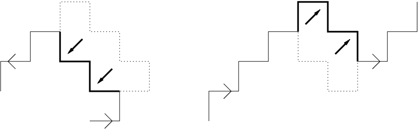
We thus have two simple zig-zag segments $\zeta_{i}$ and $\zeta_{o}$, starting respectively from $\beta_{i}$ and $\beta_{o}$ with a common edge $e$. Continue $\zeta_{o}$ as a zig-zag beyond $e$ until it hits the boundary or self-intersects. If it hits the inner boundary we are done. If it hits the outer boundary, then $\zeta_{o}$ together with a piece of $\beta_{o}$ bound a quadriculated disk into which the zig-zag continuation of $\zeta_{i}$ enters at the edge $e$. Thus, from Gauss-Bonnet, the zig-zag continuation of $\zeta_{i}$ eventually hits $\beta_{o}$ without self-intersecting or intersecting the extended $\zeta_{o}$: $\zeta_{i}$ is then the required zig-zag. Finally, if $\zeta_{o}$ self-intersects, we are in the situation of item (b) and $\beta_{o}$ has curvature $+1$. The zig-zag continuation of $\zeta_{i}$ cannot self-intersect (from (b)) and cannot intersect $\zeta_{o}$ a second time (from Gauss-Bonnet) and thus must eventually hit $\beta_{o}$ and we are done.     $\blacksquare$

We recall the basic properties of height functions for a connected and simply connected quadriculated surface $S$ with boundary ([10]; see also [9] for the minor adjustments required for surfaces with no boundary). Let ${\cal V}_{S}$ be the set of vertices of squares in $S$ and ${\cal V}_{\partial S}\neq\emptyset$ be the subset of vertices on the boundary of $S$. Call an arbitrary but fixed vertex $v_{b}\in{\cal V}_{\partial S}$ the base vertex. For a tiling $t\in T_{S}$, construct the height function $\theta:{\cal V}_{S}\to{\mathbb{Z}}$ as follows:

1. (a)

   $\theta(v_{b})=0$;

2. (b)

   if there is a white (resp. black) square to the left of the oriented edge $v_{0}v_{1}$ not covered by a domino of $t$ then $\theta(v_{1})-\theta(v_{0})=1$ (resp. $-1$).

Clearly, these rules are consistent when constructing $\theta$ along the path surrounding a domino. This local consistency, together with the fact that $S$ is connected and simply connected, yield uniqueness and global consistency of $\theta$. Notice that all height functions coincide on the boundary and that changing the base vertex alters $\theta$ by an additive integer constant. Height functions admit the intrinsic characterization below, given in strictly local terms (for a proof and some applications, see [9]).

Recall that all height functions $\theta$ with base point $v_{b}$ equal 0 at $v_{b}$. From the local characterization of height functions, given a point $v\in{\cal V}_{S}$ at a distance $\ell$ (measured along edges) from $v_{b}$, $|\theta(v)|\leq 3\ell$. Thus, even for infinite connected and simply connected quadriculated surfaces, height functions are locally bounded in the sense that given any finite subset $X$ of ${\cal V}_{S}$ the restrictions of all height functions to $X$ are bounded by a constant $C_{X}$. In particular, the maximum or minimum of any (finite or infinite) set of height functions is well defined and, again from the local characterization, is a height function. The set of height functions, and therefore the set of tilings, thus form a lattice.

Since the quadriculated annulus $A$ is not simply connected, the construction of a height function as above is not necessarily globally consistent. In [9], this difficulty is addressed by the construction of height sections. Here, we follow the simpler alternative of considering tilings in the band $A^{\infty}$, which correspond to height functions from ${\cal V}_{A^{\infty}}$ to ${\mathbb{Z}}$. For convenience, we assume the base point $v_{b}$ to belong to the outer boundary of $A^{\infty}$.

In the general case when $v_{b}$ or $v_{r}$ are not ends of $\xi_{\frac{1}{2}}$, one has to account for the variations of $\theta$ along stretches of boundary from ends to $v_{b}$ or $v_{r}$ which again are independent of tiling.     $\blacksquare$

Notice that a height function $\theta$ corresponding to a periodic tiling of $A^{\infty}$ does not usually satisfy $(\theta\circ\tau)(v)=\theta(v)$ but instead $(\theta\circ\tau)(v)=\theta(v)+c^{\prime}$ for some integer constant $c^{\prime}$; $c^{\prime}$ depends on $A$ only and not on the tiling $t$. With a slight abuse, we still call such height functions periodic. Call $\theta_{f,\max}$ (resp. $\theta_{f,\min}$) the maximum (resp. minimum) of all height functions with a given flux $f$. These extremal height functions are periodic. Indeed, from the lattice structure on the set of height functions and maximality of $\theta_{f,\max}$, it is easy to see that

where $c^{\prime}=\theta_{f,\max}(\tau(v_{b}))$.

The following result is an application of height functions to tilings of annuli.

Like walls (in Theorem 2.3), the non-trespassable cuts above allow for a multiplicative principle to be applied to the counting of tilings of extremal flux. Indeed, let $a^{[n]}_{k}$ be the number of tilings of the covering space $A^{n}$ with flux $k+f_{\min}$, $k=0,\ldots,f_{\max}-f_{\min}$; we have $a^{[n]}_{f_{\max}-f_{\min}}=(a^{[1]}_{f_{\max}-f_{\min}})^{n}$ and $a^{[n]}_{0}=(a^{[1]}_{0})^{n}$. More general relations among the $a^{[n]}_{k}$ will be presented in Proposition 5.2.

Notice that $f_{\max}-f_{\min}$ is the number of non-zero roots of $\Phi_{A}^{+}(p)$. Also, from the definition of flow relative to a cut, $f_{\max}-f_{\min}$ is less than or equal to the length of the shortest cut in $A$.

Kasteleyn ([4]) showed how to count tilings of quadriculated disks by computing a determinant; this idea has been extended by many authors, in particular by producing a matrix whose determinant $q$-counts tilings of quadriculated disks ([2]). A variation of these ideas, to be detailed in Proposition 4.6, obtains the $q$-flux polynomial $\Phi_{A}(p,q)$ for a quadriculated annulus $A$. The $q$-flux polynomial will extend the flux polynomials defined in the introduction: $\Phi_{A}^{+}(p)=\Phi_{A}(p,1)$ and $\Phi_{A}^{-}(p)=\Phi_{A}(p,-1)$.

Let $\Delta$ be a periodic track segment (as defined in Section 2), $A=\operatorname{cl}\Delta$ and $\xi$ the induced cut in $A$. The adjacency graph $G_{A}$ of the quadriculated annulus $A$ is the oriented graph whose vertices are squares of $A$ and whose edges connect squares sharing a common side, always oriented from black to white. The domino arrows of a tiling are edges in $G_{A}$. An edge crosses $\xi$ counterclockwise (resp. clockwise) if it leaves through the attachment $\alpha_{0}$ (resp. $\alpha_{1}$) and enters through $\alpha_{1}$ (resp. $\alpha_{0}$). Let $C_{1}(A)$ be the set of formal sums (with integer coefficients) of edges of $G_{A}$. Also, let $Z_{1}(A)\subseteq C_{1}(A)$ be the additive subgroup of formal sums such that at each vertex of $G_{A}$ the sum of the coefficients of the adjacent edges is zero. For example, the difference $c=t_{1}-t_{2}$ of two tilings of a quadriculated surface $A$ is an element of $Z_{1}(A)$. Following the homological terminology, the elements of $Z_{1}(A)$ are $1$-cycles.

There is a natural basis for $Z_{1}(A)$: the hole basis. Recall that $A$ and therefore $G_{A}$ are embedded in ${\mathbb{R}}^{2}$. The bounded connected components of the complement of the graph $G_{A}$ are the holes of the graph $G_{A}$: each hole gives rise to an element of the hole basis, as follows. Many holes of the graph are bounded by four edges, the small holes. The basis 1-cycle $s_{i}$ corresponding to a small hole consists of those four edges oriented counterclockwise (here a white-to-black edge is identified with minus the same edge with the original black-to-white orientation). The only remaining hole, the large hole, contains the bounded connected component of ${\mathbb{R}}^{2}-A$. To obtain the 1-cycle $\ell$ associated to the large hole, add the edges contained in the boundary of the closure of the large hole, orienting them so as to have the hole to the left. Figure 7 below represents the same basis element $\ell$ in two ways, and is given to justify the apparently convoluted definition.

As usual, a circuit in a graph is a 2-regular subgraph; thus, a circuit is a simple closed curve contained in $G_{A}$. Oriented circuits are 1-cycles and generate $Z_{1}(A)$: each $s_{i}$ is an oriented circuit and $\ell$ is a sum of disjoint oriented circuits. The decomposition in the hole basis of a circuit $c$ oriented counterclockwise is very geometric. From the region of the plane surrounded by $c$, remove $G_{A}$ to obtain a disjoint union of holes $h_{1},\ldots,h_{F}$: we clearly have $c=\sum h_{i}$.

We define three group homomorphisms by prescribing their values on the hole basis.

Given the example in Figure 7, the concept of length of $\ell$ may appear confusing. Consider the boundary of the large hole: this consists of $k_{\text{simple}}$ edges which bound the large hole on one side only and of $k_{\text{double}}$ edges which bound the large hole on both sides (in Figure 7, $k_{\text{simple}}=20$ and $k_{\text{double}}=3$). Let $2k=k_{\text{simple}}+2k_{\text{double}}$.

The definitions of flux and sign of a tiling given in the introduction are special cases of the new definitions, as will be seen in Corollary 4.3. For the moment, we provide geometric meaning to these homomorphisms.

So far, $\phi$, $\sigma$ and $\nu$ have been defined in $Z_{1}(A)$. However, in the introduction, we defined $\phi(t;t_{0})$ and $\sigma(t;t_{0})$ for a tiling $t$ relative to a base tiling $t_{0}$. We now relate this old definition of $\phi$ and $\sigma$ with the new one. Notice that a tiling $t$ does not belong to $Z_{1}(A)$ but the difference $t-t_{0}$ does.

In parallel with this corollary, we also set $\nu(t;t_{0})=\nu(t-t_{0})$, the volume of a tiling $t$ relative to a base tiling $t_{0}$. Also, the reader may check that $\phi(t;t_{0})=\phi(t,\xi)-\phi(t_{0},\xi)$ for an arbitrary cut $\xi$.

Let ${\cal A}$ a commutative algebra with unit over ${\mathbb{C}}$; in this paper, ${\cal A}$ is typically a ring of Laurent polynomials in one or two variables: ${\cal A}_{q}={\mathbb{C}}[q,q^{-1}]$ and ${\cal A}_{p,q}={\mathbb{C}}[p,p^{-1},q,q^{-1}]$. As usual, an attribution of invertible elements of ${\cal A}$, i.e., elements of the multiplicative group ${\cal A}^{\ast}$, to the edges of $G_{A}$ is a ${\cal A}^{\ast}$-weight in $A$ and turns $G_{A}$ into a weighted graph. A weight $\omega$ is thus a function from the set of edges to ${\cal A}^{\ast}$ and may naturally be identified with a homomorphism $\omega:C_{1}(A)\to{\cal A}^{\ast}$. In particular, for a tiling $t$, $\omega(t)$ is the product of the weights of the edges in $t$. An oriented circuit $c$ is the sum of its edges which are oriented black-to-white minus the sum of its remaining edges: $\omega(c)$ is the product of the weights of the edges in the first class divided by the product of the weights of the remaining edges. For a periodic track segment $\Delta$, we are interested in certain weights in $G_{A}$ for the annulus $A=\operatorname{cl}\Delta$.

Given an edge $e$ in $G_{A}$ not in the tree, there is a unique positively oriented circuit $c_{e}$ whose edges are either $e$ or edges in the tree. The relation $\omega(c_{e})=\sigma(c_{e})p^{\phi(c_{e})}q^{H(c_{e})}$, which $\omega$ must satisfy from condition (d) above, now imposes the value of the weight of $e$. This defines a weight $\omega$ on $G_{A}$.

If $e$ is in $\Delta$, then $c_{e}$ is also in $\Delta$ and therefore $\phi(c_{e})=0$: the weight assigned to $e$ thus belongs to ${\cal A}_{q}^{\ast}$, verifying condition (a). If instead $e$ crosses $\xi$ counterclockwise (resp. clockwise), we have $\phi(c_{e})=1$ (resp. $-1$), verifying in turn condition (b) (resp. condition (c)).

Set $W:Z_{1}(A)\to{\cal A}^{\ast}$ to be

References

- [1] Deift, P. A. and Tomei, C., On the determinant of the adjacency matrix for a planar sublattice, J. Combin. Theory Ser. B, 35, 278–289 (1983).
- [2] Elkies, N., Kuperberg, G., Larsen, M. and Propp, J., Alternating sign matrices and domino tilings, J. Alg. Combin. 1, 112–132 and 219–239 (1992).
- [3] Gantmacher, F. R., The theory of matrices, Chelsea Publishing Co., New York, 1977.
- [4] Kasteleyn, P. W., The statistics of dimers on a lattice, I. The number of dimer arrangements on a quadratic lattice, Physica, 27, 1209–1225 (1961).
- [5] Kasteleyn, P. W., Dimer statistics and phase transition, J. Math. Phys. 4, 287–293 (1963).
- [6] Katok, A. and Hasselblatt, B., Introduction to the modern theory of dynamical systems, Encyclopedia of Mathematics and its Applications, v. 54, Cambridge Univ. Press, 1995.
- [7] Lieb, E. H. and Loss, M., Fluxes, Laplacians and Kasteleyn’s theorem, Duke Math. J., 71, 337–363 (1993).
- [8] MacMahon, P. A., Combinatorial analysis, Chelsea Publishing Co., New York, 1960.
- [9] Saldanha, N. C., Tomei, C., Casarin, M. A. and Romualdo D., Spaces of domino tilings, Discrete Comput. Geom. 14, 207–233 (1995).
- [10] Thurston, W. P., Conway’s tiling groups, Amer. Math. Monthly 97, 757–773 (1990).
Nicolau C. Saldanha and Carlos Tomei
Depto. de Matemática, PUC-Rio
R. Mq. de S. Vicente 225
Rio de Janeiro, RJ 22453-900, Brazil
nicolau@mat.puc-rio.br
tomei@mat.puc-rio.br