\degreeyear

1999 \degreeDoctor of Philosophy \chairPeter Doyle \othermembersProfessor Bruce Driver
Professor Kate Okikiolu
Professor Zheng-xu He
Professor Kenneth Intriligator
Professor Steven Shapin \numberofmembers6 \prevdegreesB.A. University California, San Diego 199?
M.A. University of Washington, Seattle199? \fieldMathematics \campusSan Diego

Random Delaunay Triangulations, the Thurston-Andreev Theorem, and Metric Uniformization

Gregory Leibon

Abstract

In this thesis a connection between the world of discrete and continuous conformal geometry is explored. The world of discrete conformal geometry is related to disk pattern construction and triangulation production. In particular we discover a generalization of the Thurston-Andreev theorem to any angles in $(0,\pi]$ (when $\chi(M)<0$ ).. The proof of this theorem relies on an energy measuring how “uniform” the angle data of a triangulation is, where by uniform angle data I mean the data of a geodesic triangulation of a hyperbolic surface. The connection to continuous geometry is via averaging this energy over geodesic triangulations, a process which forms an energy measuring how “uniform” (constant curvature) a metric is. In fact, the entire discrete energy proof carries over to produce a proof of the metric uniformization theorem of conformal geometry. The random triangulations used to produce this averaging are random Delaunay triangulations, and they are explored in some detail. In particular the averaging techniques developed to construct the energy on metrics can be used to explore other geometric issues, including the production of a probabilistic interpretation of the determinant of the Laplacian and a new probabilistic proof of the Gauss-Bonnet theorem.

\copyrightpage\degreeyear

1999 \approvalpage{dedication}

To Squirl

Acknowledgements.

I’d like to acknowledge that the story I present here would not exist without my thesis advisor Peter Doyle, and his inspired view of mathematics. It was his sense of esthetics and understanding that led to the conjectured mathematical stories for which this thesis is a confirmation. Trying to understand Peter’s world was a huge part of my inspiration to become a part of mathematics and I can’t thank him enough for sharing so many of his beautiful ideas with me over the years. Thanks Peter! UCSD was a wonderful community to do mathematics in, largely due to the huge number of supportive people, and I thank you all. I would especially like to thank Bruce Driver, Jay Fillmore and Jeff Rabin for their many years of support and mathematical inspiration. I would also like to thank Kate Okikiolu and Zheng-xu He for the insights they have provided into the story presented here. I’d also like to thank all my fellow graduate students who over the years have listened to my rantings and given sound advice or a good kick in the butt. I’d also like to thank Dave Collingwood and my master’s thesis advisor John Lee at the University of Washington for their support; as well as my Washington math buddies Steve, Mike, Dave and Siva for showing me lots of neat stuff and being great friends. I’d especially like to thank Albert Nijenhuis of University of Washington for his wonderful comments and his beautiful proof of the small circle intersection theorem which appears in chapter 3. I would also like to thank my outside committee members Steven Shapin and Ken Intriligator (as well as my inside department committee members) for putting up with my poor planning abilities and general silliness. On this note a HUGE thanks goes out to Lois Stewart for saving my butt many many times; I certainly would have been kicked out of UCSD long before completing my thesis if not for her watchful eye. The biggest thanks of all goes to my wife Nicole, for always being so supportive and never letting me lose track of what’s really important in life.

{vitapage}{vita}

B.A., summa cum laude, University of California San Diego

Teaching assistant, Department of Mathematics, University of Washington Seattle

M.S., University of Washington Seattle

Mathematics Instructor, Department of Mathematics, University of Washington Seattle

Teaching assistant, Department of Mathematics, University of California San Diego

Associate Instructor, Department of Mathematics, University of California San Diego

Ph. D., University of California San Diego {publications}

The ideal Thurston-Andreev theorem and triangulation production. In Preparation.

Random Delaunay triangulations and metric uniformization. In Preparation.

Delaunay triangulation of a surface. In Preparation.

Chapter 0 Introduction

It has been known for a while now that the world of disk patterns is intimately connected to the world of geometric uniformization. To orient ourselves to what this statement means it is useful to mention the most famous case. The disk pattern is the Koebe theorem which guarantees that a specified (reasonably nice) graph embedded in the closed unit disk can be realized as the nerve of a disk pattern, which is in fact unique up to Möbius equivalence. In [18] Thurston presented the idea of (nicely) packing a bounded simply connected planar domain, recording the nerve of this packing, and then using a suitably normalized solution to the Koebe disk pattern with respect to this nerve in order to approximate the conformal mapping of this region to the disk. That such a mapping exits is our first example of a geometric uniformization problem, the Riemann mapping theorem. Thurston’s procedure has been verified to work in several cases. In fact this conjecture has been solved in several cases. The case of using a finer and finer hexagonal disk pattern for the approximation is very well understood; it was first shown to uniformly approximate the Riemann mapping in [16] and is now seen in [10] to approximate uniformly all of the Riemann mapping’s derivatives.

In this thesis another connection between these two stories is developed. For now I’ll give a brief outline which can be viewed as an introduction to the introduction. Precise statement of the below discussion can be found in the elaborated introduction, sections 1.1 - 1.3.

In this thesis a generalization of a disk pattern theorem often called the Thurston-Andreev theorem is presented, which is the solution to a disk pattern problem on a compact surface. To be precise, in chapter two of this thesis we prove…

Result 1

Given a geodesic triangular decomposition of a hyperbolic surface one can associate combinatorial data: the topological class of the triangular decomposition and to each edge the angle between the circumscribing circles of the two triangles sharing the edge. If the angle data is in $(0,\pi]$ then this combinatorial data uniquely determines both the hyperbolic structure and the geodesic triangulation. Furthermore, if one starts with a topological triangular decomposition of a compact surface with $\chi(M)<0$ , and angles with values in $(0,\pi]$ assigned to each edge satisfying certain necessary linear conditions (conditions $(n_{1})$ – $(n_{4})$ of section 1), then there is a hyperbolic surface and geodesic triangular decomposition realizing this data.

The angles in $(0,\frac{\pi}{2}]$ case is well known, see [17]. This theorem has several interpretations in terms of not only a disk pattern problem, but also as a convex hyperbolic polyhedron production theorem, and perhaps most importantly (from the uniformization point of view) as a geodesic triangulation production theorem. This triangulation production can be viewed as the second step in the proof of the above result. The first step is a completely linear max-flow-min cut-type problem guaranteeing that given such edge angle data one can produce triangle angle data which “formally” has the same edge angle data associated to it. Given such triangle angle data one can measure how uniform this data is by using an energy on the set of possible conformally equivalent angle data. This energy is larger when one is closer to the angle data of a geodesic triangulation of a hyperbolic surface (so for aesthetic reasons I’ve chosen an energy which one tries to maximize, my apologies to the physicists). The proof becomes to guarantee the existence of a unique set of angle data maximizing this energy and to show it corresponds to the unique solution of the above disk pattern result.

The geometric uniformization theorem which this result will be shown intimately related to, is the uniformization for geometric surfaces, namely:

Result 2

Every Riemannian surface is conformally equivalent to a Riemannian surface with constant Gaussian curvature.

This theorem is very well known. The heart of what takes place here is that in chapter 4 there is a proof of the above uniformization theorem which is directly related to the above disk pattern theorem and its proof. This relationship is to first (as above) solve the completely linear problem of finding a varying negative curvature metric, then we can measure how distant this metric is from a constant curvature metric by averaging the energy associated to data provided by randomly selected triangulations. In the end one finds the same arguments used to uniformize the discrete angle data can be applied to this averaged energy on the space of metrics, providing a nice proof of the uniformization theorem of surfaces. This is not the first energy method proof of this theorem, in fact there are many. One particularly interesting energy is the $det(\Delta_{g})$ as used in [2]. In fact these random energies are related to the $det(\Delta_{g})$ , and in section 1.3 this relationship is made explicit.

The main tool in articulating the averaging procedure is a detailed understanding of random Delaunay triangulations. The details of this understanding form chapter 3. I think these triangulations are quite interesting independent of their connection to metric uniformization, and I hope to convince others of this by beginning the precise introduction with a probabilistic proof on the Gauss-Bonnet theorem.

It is worth noting that these ideas may be explored in three-dimensions. In fact much of what takes place here can be viewed as realization in two dimensions of an idea by Peter Doyle to prove that a three manifold accepting a varying negative curvature metric also accepts a constant sectional curvature metric. If proved this result would shed considerable light on Thurston’s uniformization conjecture. In section 1.3 I sketch the three dimensional strategy, as related to the two dimensional strategy presented in 1.1-1.2.

1 A New Proof of the Gauss-Bonnet Theorem

The Gauss-Bonnet formula in its most primitive form is stated for a compact boundaryless surface endowed with a geometry as:

\frac{1}{2\pi}\int_{M}kdA=\chi(M).

The quantity, $k$ , being integrated over the surface, $M$ , is the Gaussian curvature, and on the right-hand side is the Euler Characteristic. The Euler characteristic is a topological invariant of the surface which can be computed from triangulation as

\chi(M)=V-E+F,

where $V$ is the number of vertices, $E$ is the number of edges, and $F$ is the number of faces in the triangulation. In a somewhat unintelligible nut shell, the proof here is accomplished by randomly triangulating the surface and then noting while the Euler characteristic is constant the other (now random variables) $E$ , $F$ , and $V$ have expected values which can be computed and compared to this constant. As the density of the randomly distributed vertices goes to infinity one finds these expected values produce the Gauss-Bonnet formula, along with a probabilistic interpretation of curvature.

This proof’s initial need is an articulation of what a random triangulation of a surface is. The first step is to ignore the fact that anything random is going on here and to simply attempt to construct a a geodesic triangulation in a fixed metric $g$ from a given set of points, ${\bf p}=\{p_{1},...,p_{n}\}$ . To do this one examines all the triples and pairs in $\{p_{1},...,p_{n}\}$ and decides whether or not to put in a face for a given triple or an edge for a given pair; this decision procedure will be relative to a certain positive number $\delta$ – the decision radius. The procedure (with its origin found in Delaunay’s “empty sphere” method, see [5]) is to formally put in a face for a triple or an edge for a pair if the triple or pair lies on a disk of radius less $\delta$ which has its interior empty of points in $\{p_{1},...,p_{n}\}$ . Clearly every pair on a face forms an edge (though not necessarily the converse), hence at this moment we have an abstract two complex. Call this abstract complex $K_{\{p_{1},...,p_{n}\}}$ and denote a polyhedral realization as $|K_{\{p_{1},...,p_{n}\}}|$ (for a realization of it place the points at $(0,\dots,0)$ and $(0,\dots,0,1,0,\dots,0)$ in $\bf{R}^{n-1}$ and take the convex hull of the subsets found in $K_{\{p_{1},...,p_{n}\}}$ ).

Our goal now is to realize this polyhedron inside the surface, which will involve restricting $\delta$ . To get going we must recall a well known geometric constant associated to the surface, the injectivity radius, which is the largest number $i$ such that if $d(p,q)<i$ then there is a unique geodesic between $p$ and $q$ of length less than $i$ . If one assumes that $\delta<\frac{i}{6}$ one can (see the proof of 1) produce a continuous map

R:|K_{\{p_{1},...,p_{n}\}}|\rightarrow M,

with the edges parameterizing geodesics in the $g$ metric. That our procedure forms a triangulation is now equivalent to $R$ being a homeomorphism; and in such a case we will call the resulting triangulation a Delaunay triangulation. Such triangulations typically will look locally like figure 1.

Refer to caption — Figure 1: Part of a Typical Delaunay Triangulation

At this point it is useful to find a geometric criterion on a set of points ${\{p_{1},...,p_{n}\}}$ guaranteeing that it forms a triangulation. To accomplish this it is useful to recall a second geometric constant associated to the surface: the strong convexity radius $\tau$ . On a compact surface it is the largest number with the property that in a disk of radius less than $\tau$ the interior of the unique minimal length geodesic connecting any pair of points in the disk’s closure is in the disk’s interior. We may now introduce our criterion for triangulation detection: we will call a set of points ${\{p_{1},...,p_{n}\}}$ $\delta$ -dense if each open ball of radius $\delta$ contains at least one $p_{i}$ and ${\{p_{1},...,p_{n}\}}$ contains no four of its points is on a circle of radius less than $min\{\frac{i}{6},\tau\}$ . With this concept we will prove in section 2.2 the following theorem…

Theorem 1

If ${\{p_{1},...,p_{n}\}}$ is $\delta$ -dense with $\delta\leq min\{\frac{i}{6},\tau\}$ , then ${\{p_{1},...,p_{n}\}}$ forms a Delaunay triangulation.

From here on out always assume the decision radius $\delta$ satisfies $\delta\leq min\{\frac{i}{6},\tau\}$ .

Now comes the second step in this proof: to put down random sets of points. The points will be distributed with a density $\lambda$ via a Poisson distribution relative to $g$ (developed in the section 2.3), and it is convenient to also randomly select an ordering of the points after placing them down. In technical terms, any such point configuration will be denoted p and will live in a measure space $\bf{P}$ with a probability measure $\bf P_{\lambda}$ and specified measurable sets $\bf B$ - all of which are constructed in section 2.3. For now all we need to understand are certain basic properties and terminology. Let $U\subset M$ be measurable with area $A(U)$ . The first property is the characteristic property of the Poisson distribution, namely the set of point configurations in $\bf{P}$ with exactly $n$ points in $U$ is an element of $\bf B$ with measure $\frac{{(A(U)\lambda)}^{n}e^{-\lambda A(U)}}{n!}$ .

Recall a random variable on $\bf P$ is simply a $\bf B$ measurable function. We will encounter several in this proof, namely $E({\bf p})$ , $V({\bf p})$ , $F({\bf p})$ , and the characteristic (indicator) functions of various measurable sets (denoted $1_{U}$ with $U$ measurable). The expected value of a random variable $L({\bf p})$ is the integral of the function over $\bf P$ with respect to the measure $\bf P_{\lambda}$ , and will be denoted $\bf E_{\lambda}(L)$ . As an example of such an expected value, using $A$ to denote the area on $M$ , we have from the above characteristic property

\bf E_{\lambda}(V)=\sum_{n=0}^{\infty}n\frac{A^{n}\lambda^{n}}{n!}e^{-A\lambda}=A\lambda\sum_{n=1}^{\infty}\frac{{(A\lambda)}^{n-1}}{(n-1)!}e^{-A\lambda}=A\lambda,

which reveals the use of the term density for $\lambda$ . The most important set for us in $\bf P$ is the set $\bf T_{\delta}\subset\bf P$ consisting of configurations which have Delaunay triangulations associated to them. By theorem 1, when our points are put in with a high density we expect they will typically form Delaunay triangulations. Allowing $O(\lambda^{-\infty})$ to mean a quantity decaying faster than any polynomial in $\lambda$ , in section 2.3 we prove this with:

Theorem 2

If $L$ is any one of $1_{\bf T_{\delta}}$ , $E$ , $V$ , or $F$ , then $L$ is measurable and has expected value $\bf E_{\lambda}(L)=\bf E_{\lambda}(L1_{\bf T_{\delta}})+O(\lambda^{-\infty})$ .

Now one observes that the Euler characteristic of any configuration in $\bf T_{\delta}$ is the Euler characteristic of an actual triangulation, hence the constant $\chi(M)$ ; so along with the above theorem 2 one has

\chi(M)=\bf E_{\lambda}(\chi(M)1_{\bf T_{\delta}})+O(\lambda^{-\infty})=\bf E_{\lambda}((V-E+F)1_{\bf T_{\delta}})+O(\lambda^{-\infty}).

Applying the mathematical triviality, yet philosophical miracle, that expected values add gives us

\chi(M)=\bf E_{\lambda}(V1_{\bf T_{\delta}})-\bf E_{\lambda}(E1_{\bf T_{\delta}})+\bf E_{\lambda}(F1_{\bf T_{\delta}})+O(\lambda^{-\infty}).

In an actual triangulation we have $\frac{3}{2}E=F$ so

\chi(M)=\bf E_{\lambda}(V1_{\bf T_{\delta}})-\frac{3}{2}\bf E_{\lambda}(F1_{\bf T_{\delta}})+\bf E_{\lambda}(F1_{\bf T_{\delta}})+O(\lambda^{-\infty}).

As explored above, we have the expected number of vertices is $\lambda A$ ; this along with theorem 2 gives us

\chi(M)=A\lambda-\frac{1}{2}\bf E_{\lambda}(F1_{\bf T_{\delta}})+O(\lambda^{-\infty}).

So finally using theorem 2 one last time we find:

Formula 1 (Euler-Delaunay-Poisson Formula)

\chi(M)=\lim_{\lambda\rightarrow\infty}\left(A\lambda-\frac{1}{2}\bf E_{\lambda}(F)\right).

The goal now becomes to compute $\bf E_{\lambda}(F)$ . Now a triple of points occurring in a Poisson configuration, $y\in M\times M\times M$ , forms a face exactly when one of its associated disks is empty of points. The first thing we’d like is that we are in fact talking about a unique such disk. This is the most sophisticated fact needed, and occurs throughout the proof. I’ll record it here for future reference; for a couple of proofs see [12]:

Lemma 1 (The Small Circle Intersection Lemma)

If a triple of points lies on a the boundary of a disk with radius less than $\delta$ , then this disk is unique among disks of radius less than $\delta$ . (Recall $\delta\leq min\{\frac{i}{6},\tau\}$ .)

Back to the computation, by the characteristic property of the Poisson distribution the probability any area $a$ disk is empty is $e^{-\lambda a}$ . So letting $V_{\delta}\subset\times^{3}M$ be the set of ordered triples living on circles of radius less than $\delta$ , we now see the probability that $y$ has an associated face should be $\frac{1}{A^{3}}\int_{V_{\delta}}e^{-\lambda a(y)}dA^{3}$ , with $a(y)$ the area of $y$ ’s uniquely associated disk. This together with the fact that the expected number of triples is $\sum_{n=0}^{\infty}\binom{n}{3}\frac{{(A\lambda)}^{n}e^{-\lambda A}}{n!}=\frac{{(A\lambda)}^{3}}{6}$ leads one to hope, as is confirmed in the beginning of section 3, that

\displaystyle\bf E_{\lambda}(F)=\frac{{\lambda}^{3}}{6}\int_{V_{\delta}}e^{-\lambda a(y)}dA^{3}.

(1)

To compute this explicitly it is necessary to put coordinates on $V_{\delta}$ . First one chooses a way to discuss directions at all but a finite number of tangent planes of $M$ (via a orthonormal frame). Then one can parameterize a full measure subset of $V_{\delta}$ with a subset of $(\theta_{1},\theta_{2},\theta_{3},r,p)\in S^{1}\times S^{1}\times S^{1}\times(0,\delta)\times M$ by hitting the triple described by sitting at the point $p\in M$ and moving a distance $r$ in each of the three directions $\theta_{1}$ , $\theta_{2}$ , and $\theta_{3}$ . That this is a legal parameterization is easily deduced from lemma 1, and discussed in section 2. Note that when fixing $p$ and varying $\theta_{i}$ in these coordinates one produces the Jacobi field $J_{i}(r)$ ; whose norm I will call $j_{i}$ . Using this notation, letting $d\vec{\theta}=d\theta_{1}\wedge d\theta_{2}\wedge d\theta_{3}$ , and letting $\nu(\vec{\theta})$ be the area of the triangle in the Euclidean unit circle with vertices at the points corresponding to the $\{\theta_{i}\}$ , we will see in section 3.1 that equation (1) expressed in these new coordinates is

\displaystyle\frac{\lambda^{3}}{6}\int_{M}\int_{0}^{\delta}\int_{\times^{3}S^{1}}e^{-\lambda a(\vec{\theta},r,p)}j_{\theta_{1}}j_{\theta_{2}}j_{\theta_{3}}\nu(\vec{\theta})d\vec{\theta}drdA.

(2)

Both $j_{i}$ and the area of a ball function, $a(\vec{\theta},r,p)$ , are directly related to the curvature; with this relationship equation 2 can be expressed as

\displaystyle\frac{\lambda^{3}}{6}\int_{M}\int_{0}^{\delta}\int_{\times^{3}S^{1}}e^{-\lambda\pi r^{2}}\nu(\vec{\theta})\left(r^{3}-\frac{k}{2}r^{5}+\frac{\pi\lambda k}{12}r^{7}+``O"(r^{6})\right)d\vec{\theta}drdA,

(3)

with the $``O"(r^{6})$ a well controlled function of $\vec{\theta}$ , $r$ , $p$ and $\lambda$ . In fact the $``O"(r^{6})$ term is so controlled that there is a $\rho_{M}>0$ associated to the surface such that if $\delta<\rho_{M}$ after integrating one can reduce equation 3 to

\displaystyle\bf E_{\lambda}(F)=2A\lambda-\frac{1}{\pi}\int_{M}kdA+O(\lambda^{-\frac{1}{2}}),

(4)

with the $|O(\lambda^{-\frac{1}{2}})|\leq C\lambda^{-\frac{1}{2}}$ (see section 3 for the details concerning 3 and 4 and the related estimates).

In particular we may now plug this into the Euler-Delaunay-Poisson Formula (formula 1) to give simultaneously a probabilistic interpretation of curvature and new proof of the Gauss-Bonnet theorem.

Formula 2 (Euler-Gauss-Bonnet-Delaunay Formula)

Using a decision radius $\delta<\rho_{M}$ we have

\chi(M)=\lim_{\lambda\rightarrow\infty}(A\lambda-\frac{1}{2}\bf E_{\lambda}(F))=\frac{1}{2\pi}\int_{M}kdA.

Note this allows us to interpret the Gaussian curvature as the defect in the expected number of faces in a random Delaunay triangulation in the surface’s geometry from what would be expected in Euclidean space.

2 Conformal Geometry and Uniformization

The techniques used in the previous section to prove the Gauss-Bonnet theorem can be used to examine certain aspects of conformal geometry. The ideas will involve the comparison of conformally equivalent metrics. In terms of Riemannian metrics we say two metrics on $M$ , $g$ and $h$ , are conformally equivalent if $h=e^{2\phi}g$ for a smooth function $\phi$ . We will always be thinking in terms of a fixed background metric called $g$ and will label its associated geometric objects like its gradient, Laplacian, curvature, norm, area element, or area as $\nabla$ , $\Delta$ , $k$ , $|\cdot|$ , $dA$ or $A$ . For the $h=e^{2\phi}g$ metric we shall denote these object with an $h$ subscript.

The key to using the ideas of the previous section is the development of a discrete analog of a conformal structure and a conformal transformation relative to a Delaunay triangulation. The most important observations in guessing this discrete structure concerns two triangles $t_{1}$ and $t_{2}$ in a Delaunay triangulation sharing an edge $e$ , and the intersection angle $\theta^{e}$ between the circles in which $t_{1}$ and $t_{2}$ are inscribed (see figure 2). The facts of use to us are that $\theta^{e}\in(0,\pi)$ and $\theta^{e}$ is preserved under a conformal deformation of the metric up to order $O(r)$ (see formula 29 in section 1).

To use this information it is necessary to note $\theta^{e}$ can be written down accurately in terms of the angles within the triangles.

Formula 3

Letting $A^{i}$ , $B^{i}$ and $C^{i}$ be the angles in $t_{i}$ as in figure 2 we have

\theta^{e}=\frac{\pi+A^{1}-B^{1}-C^{1}}{2}+\frac{\pi+A^{2}-B^{2}-C^{2}}{2}+O(r^{3}).

It is worth noting this formula is exactly true on a surface with constant curvature. One proof of this formula in the negative curvature case utilizes an object, an ideal hyperbolic prism, that will turn out to be fundamental to all that takes place here; and it is useful to construct and discuss it now. That it shows up at such a fundamental point in understanding the triangulations will hopefully inspire its otherwise unexpected appearance in the next section.

The prism is constructed from the angle data of a hyperbolic triangle, namely a set of positive angles $\{A,B,C\}$ such that $A+B+C-\pi<0$ . To construct it first form a hyperbolic triangle with the $\{A,B,C\}$ data, then place the triangle on a hyperbolic plane and then place the plane in hyperbolic three space. Now union this triangle with the geodesics perpendicular to this 2-plane going through the vertices of the triangle. The prism of interest is the convex hull of this arrangement, See figure 3.

With these conformal geometry facts in mind we may set up our discrete conformal geometry.

1 Discrete Uniformization

The discrete object replacing a metric is the information naturally associated to a Delaunay geodesic triangulation living on the surface in this metric; namely a topological triangulation, $\bf{T}$ , and the angles in all the triangles. Given $\bf{T}$ there are $3F$ slots $\{\alpha_{i}\}$ in which one can insert possible triangle angles, which we will place an order on and identify with a basis of a $3F$ dimensional real vector space. With this basis choice we will denote this vector space as $\bf R^{3F}$ , and denote vectors in it as $x=\sum A^{i}\alpha_{i}$ . Let $\alpha^{i}$ be a dual vector such that $\alpha^{i}(\alpha_{j})=\delta_{i}^{j}$ . Sometimes we will refer to the angles in a fixed triangle, and will abuse notation in order to refer to figure 2 by letting $\alpha^{i}(x)=A^{i}$ , $\beta^{i}(x)=B^{i}$ , and $\gamma^{i}(x)=C^{i}$ .

We will require that these angles satisfy certain requirements that the angles in an actual Delaunay triangulation would satisfy. In particular we require that all the angles are in $(0,\pi)$ and that the sum of all the angle at a vertex is $2\pi$ .

Motivated from the previous section we define the intersection angle at an edge to be the function

\theta^{e}(x)=\frac{\pi+A^{1}-B^{1}-C^{1}}{2}+\frac{\pi+A^{2}-B^{2}-C^{2}}{2},

with the notation inspired from figure 2. The Delaunay quality is reflected in the fact that the “intersection angles” must satisfy $\theta^{e}(x)\in(0,\pi)$ for each edge $e$ . It is worth noting that as an immediate consequence of the fact that the angles sum to $2\pi$ at a vertex we have that the angle discrepancies at a vertex $\pi-\theta^{e}(x)$ sums to $2\pi$ at a vertex as well, see section 1.

We will call angles satisfying the above requirements a Delaunay angle system. With the previous section as motivation, we define a pair of Delaunay angle systems $x$ and $y$ to be conformally equivalent if they arise form the same triangulation and if for each edge $e$ the $\theta^{e}(x)=\theta^{e}(y)$ .

Motivated by the Gauss-Bonnet theorem we define the curvature of a triangle $t$ relative to the Delaunay angle system $x$ to be $k^{t}(x)=A+B+C-\pi$ , where $\{A,B,C\}$ is the angle data corresponding to angle slots in $t$ . On a surface with $\chi(M)<0$ there is a very simple set of linear equations which will gaurentee that a Delaunay angle system is conformally equivalent to a Delaunay angle system where each triangle has negative curvature.

Let $S$ be a set of triangles in $\bf{P}$ , and denote the cardinality of $S$ as $|S|$ . Let condition ( $\star$ ) on a set of angles $\{\theta^{e}(x)\}$ associated to all the edges of $\bf{P}$ be the condition that for any set of triangles $S$ we have

$(\star)$ $\sum_{e\in S}\theta^{e}(x)>\pi|S|.$

As an immediate consequence of theorem 9 we have the following lemma.

Lemma 2 (The Discrete Teleportation Lemma)

A Delaunay angle system $x$ has $\{\theta^{e}(x)\}$ satisfying $(\star)$ if and only if $x$ is conformally equivalent to a negative curvature Delaunay angle system.

We will only be concerned with Delaunay angle systems satisfying the the conditions of this lemma, which note includes the angle data associated to a Delaunay triangulation of surface with varying negative curvature. Denote the convex bounded set of negative curvature angle systems conformal to a given one, $x$ , as $\bf{N}_{x}$ .

The pleasure derived from the Delaunay angle systems comes from a beautiful Energy which lives on $\bf{N}_{x}$ . Let $V^{t}(x)$ denote the volume of the ideal hyperbolic prism constructed from $t$ ’s angle data relative to $x$ , as described in the previous section. Now simply let the energy be

E(x)=\sum_{t\in\bf{P}}V_{t}(x).

The points where $E$ attains a maximum will be of great interest to us. It is worth noting that $E$ is a continuous function on the compact set $\bar{\bf{N}}_{x}$ , so attains its maximum. In fact it is an immediate consequence of lemma 5 in section 4 that the angle system with maximal energy is in fact in $\bf{N}$ . An understanding of this as well as the energies behavior at critical points comes from understanding its differential. To interpret it let $a$ , $b$ and $c$ denote the edge lengths opposite to the angle $A$ , $B$ , and $C$ in the hyperbolic triangle determined by the angle data $\{A,B,C\}$ (which once again exists since $k^{t}(x)<0$ ). In formula 8 of section 4 the following formula is produced:

Formula 4

$dE^{x}=\sum_{\alpha_{i}\in\bf{T}}E_{i}(x)\alpha^{i}$ with

E_{i}(x)=\frac{1}{2}\left(\ln\left(\frac{\cosh(a)-1}{2}\right)-\ln\left(\frac{\cosh(b)-1}{2}\right)-\ln\left(\frac{\cosh(c)-1}{2}\right)\right),

where $\alpha^{i}(x)=A$ , $\alpha_{i}\in t$ , $t$ ’s angle data is $\{A,B,C\}$ , and the $a$ , $b$ , and $c$ are determined as above.

In order to best exploit this formula it is necessary to note (see the proof of corollary 1 in section 4) that the tangent space at any point of $\bf{N}_{x}$ can be described explicitly as the translation to that point of the span over all edges of the vectors

w_{e}=\gamma_{1}+\beta_{1}-\left(\gamma_{2}+\beta_{2}\right)

as in figure 2. The loveliness of this energy can now be expressed in terms the following observation about its critical points (i.e. where $dE=0$ ).

Observation 1

From the above formula and the above description of $T_{p}(\bf{N}_{x})$ we see at a critical point $x$ of the energy in a conformal class satisfies

0=dE(w_{e})=\ln\left(\frac{\cosh(a_{2})-1}{2}\right)-\ln\left(\frac{\cosh(a_{1})-1}{2}\right),

for all edges $e$ with the notation coming form as usual from figure 2. Hence at a critical point of $E$ we have that $a_{1}=a_{2}$ and the set of $-1$ curvature triangles formed from the given angle data fit together to form an actual constant curvature surface.

I will call the Delaunay angle system of such a critical point a uniform angle system. The question becomes: how many (if any) uniform structures can be associated to a given angle system? From above we know there is at least one internal maximum and in fact $E$ is strictly concave down (see lemma 4 in 4). So any critical point is a maximum and unique, as needed.

Theorem 3 (Discrete Uniformization Theorem)

If $\chi(M)<0$ and $x$ is a Delaunay angle system where $\{\theta^{e}(x)\}$ satisfies $(\star)$ then $x$ is conformally equivalent to a unique uniform angle system.

It is worth noting that there is a rephrasing of the above uniformization construction in terms of a solution to a disk pattern problem, namely as a corollary of theorem 9 in section 1

Theorem 4

If one is given a topological triangulation of a surface with $\chi(M)<0$ and a set $\{\theta^{e}\}$ associated to the edges satisfying both condition $(\star)$ and that at each vertex $\sum_{\{e\in v\}}\pi-\theta^{e}=2\pi$ , then there is a uniquely associated constant curvature surface on which the given triangulation is realized as a geodesic triangulation and the circles in which the triangles live meet with the specified $\theta^{e}$ angles.

Solutions to problems similar to this are well known. The first solution to such a pattern problem goes back to Koebe and pattern problems closely related to the above corollary were implicit in the work of Andreev [1] and then rediscovered and articulated in this language by Thurston (see [17]).The above theorem (actually a generalization of it found in 1) is a generalization to arbitrary angles of the convex ideal case of the Thurston-Andreev theorem. The first solutions to these pattern problems using energy methods (as far as I’m aware) can be found in [4], and energy methods using hyperbolic volumes (in the toroidal case) have there earliest versions in [3] and later in [14].

2 Continuous Uniformization

Now we’d like to mimic the uniformization procedure in the previous section for metrics. For metrics by uniform structure I will mean a metric $e^{2\phi}g$ with constant curvature. It is useful to note that $k_{h}=e^{2\phi}(-\Delta\phi+k)$ .

For starters let us note in the metric world we still have

Lemma 3 (The Metric Teleportation Lemma)

Every metric on a surface is conformally equivalent to a metric with either negative, positive , or zero curvature.

Proof: This is a consequence of the Fredholm alternative, which says if $f\in C^{\infty}(M)$ satisfies $\int_{M}fdA=0$ then $f\in\Delta(C^{\infty}(M))$ . Since $\int_{M}(k-2\pi\chi(M))dA=0$ we have there is a smooth $\phi$ satisfying $\Delta\phi=k-2\pi\chi(M)$ and hence $k_{\phi}=e^{2\phi}(-\Delta\phi+k)=2\pi\chi(M)e^{2\phi}$ as required.

q.e.d

With this observation in our $\chi(M)<0$ world we will restrict our attention to metrics with strictly negative curvature. It is worth noting that as in the discrete teleportation lemma the problem is linear.

Now given a varying negative curvature metric $h$ if we chose a ${\bf p}=\{p_{1},\dots,p_{n}\}$ and topological triangulation $K_{\bf p}$ with ${\bf p}$ as vertices then we could measure how close to uniform $h$ is with the energy of the previous section. Namely we could let

{\bf E}_{h}({\bf p})=\sum_{t\in K_{\bf p}}V^{h}_{t}({\bf p}),

where $V^{h}_{t}({\bf p})$ is computed using the angle data associate to the “triangulation” viewed in the $h$ metric. This of course means connecting the needed vertices of ${\bf p}$ with $h$ geodesics and measuring the resulting $h$ angles. Notice this makes sense for sufficient $h$ dense points since by the Gauss-Bonnet theorem for geodesic triangles the angles in a triangle $\{A,B,C\}$ will indeed satisfy

k^{t}({\bf p})=A+B+C-\pi<0.

This gives us a measurement of uniformity relative to $\{\bf p\}$ and $K_{\bf p}$ and to rid this dependency it is natural to average this measurement over all complexes as in section 1. To do so weight the point distribution and decide how to form the complexes using a fixed metric $g$ and density $\lambda$ , and then compute $\bf E_{\lambda}({\bf E}_{h})$ . It’s worth noting that it may be necessary to shrink the decision radius down a bit to make sense out of this construction, since we’d like points in a triple to be within the injectivity radius of each other in both metrics. As with the random variables of section 1 this random variable is naturally expressed as the sum over all the faces $t\in K_{\bf p}$ of a function dependent only on the data associated to an individual face, so we would expect the computations of 1 to go through.

It is clear that the higher the vertex density the higher the percentage of triangulations involved, hence the more sensitive this energy should be to measuring the uniformity of the curvature. With this as inspiration we proceed as with as with our Euler characteristic computation and take the limit as the density of vertices goes to infinity. Let

E(h)=\lim_{\lambda\rightarrow\infty}\bf E_{\lambda}({\bf E}_{h}-{\bf E}_{g}),

and note the second term ${\bf E}_{g}$ is independent of $h$ and needed only to normalize the computation. We will show that among $h=e^{2\phi}g$ with with $k_{h}<0$ this formula is equivalent to

\displaystyle E(h)=-\int_{M}||\nabla\phi||^{2}+(\Delta\phi-k)\ln(\Delta\phi-k)+k\ln|k|dA.

(5)

The energy is clearly scale invariant and $k_{h}=e^{-2\pi}(-\Delta\phi+k)$ , so we see that it is natural to consider the energy as a function on the “energy norm” closure of

V=\{\phi\in C^{\infty}\mid\int_{M}\phi dA=0\mbox{ and }-\Delta\phi+k<0\}.

Using the energy norm allows us to use compactness arguments to gaurentee the existence of a maximum, just as in the discrete case (for the details of everything that takes place in this section see section 2). Also as in the discrete we can easily force the maximum into the the interior (where $esssup(-\Delta+k)<0$ ). This requires looking at the energy’s Frechét differential, which is quite revealing.

Formula 5

The Frechét derivative of $E$ at $\phi$ in the direction $\psi$ is

DE(\psi)=-\int_{M}\Delta\psi\ln|k_{e^{2\phi}g}|dA.

This formula for Frechét derivative guarantees that $k_{h}$ is constant and $\phi$ is smooth. The easiest way to understand this is to recall the Fredholm Alternative described in the poof of lemma 3 and observe…

Observation 2

The above formula insures us that if we knew the critical $\phi$ to be a $C^{\infty}$ function then $\ln|k_{h}|$ would $L^{2}$ orthogonal to the image of $C^{\infty}(M)$ under the Laplacian, so by the Fredholm alternative $\ln|k_{h}|$ is constant. Hence we indeed see that a critical point of $E$ should be a metric of constant negative curvature.

Just as in the discrete case at this point concavity comes to the rescue to gaurentee uniqueness. Since everything is $C^{\infty}$ we really can use the fact that the Frechét Hessian at $\phi\in V$ applied to $(\psi,\psi)$

\displaystyle D^{2}{\bf}E(\psi,\psi)=-\int_{M}|\nabla\psi|^{2}+\frac{(\Delta\psi)^{2}}{\Delta\phi-k}dA_{0}

(6)

is strictly negative at a non-zero $\psi$ to gaurentee the critical point is in fact unique.

So just as in the discrete case we arrive at the uniformization theorem (although only when $\chi(M)<0$ ).

Theorem 5 (The Metric Uniformization Theorem)

Every metric is conformally equivalent to a unique metric of constant curvature.

3 The Determinant of the Laplacian and Entropy

The use of energies to solve the uniformization problem is not at all new, and it is nice to relate this process to some other more familiar energies. The method of producing other energies is to average over metrics using the varying metric to distribute the points. So in this section I will superscript the expected values with the metric used to construct the point distribution.

The first variant I will describe has the advantage of not needing to be restricted to a conformal class. It involves a function on the space of metrics I call the entropy

H(h)=\int_{M}k_{h}\ln|h_{h}|dA_{h}.

The fact is that

E_{1}(h)=\lim_{\lambda\rightarrow\infty}(\bf E^{h}_{\lambda}({\bf E}_{h})-\bf E^{g}_{\lambda}({\bf E}_{g}))=H(h)-H(g).

So viewing $g$ as fixed we have an energy on all metrics - which can be checked to optimize at a constant curvature metric and be strictly concave down in a conformal class.

More interestingly is the following energy.

Theorem 6

There is a constant $C$ such that on the set of all metrics $h$ conformally equivalent to $g$ of a fixed area

E_{2}(h)=E_{1}(h)-E(h)=\lim_{\lambda\rightarrow\infty}(\bf E^{h}_{\lambda}({\bf E}_{h})-\bf E^{g}_{\lambda}({\bf E}_{h}))=\ln(\det(\Delta_{h}))+C.

As we shall see in section 2, the key to being able to make this interpretation is the beautiful integral formulation of the $\ln(\det(\Delta_{g}))$ due to Polyakov (see [13]). The $\ln((det(\Delta_{g}))$ was found to have the uniformization property by Osgood, Phillips, and Sarnak (see [2]). In [4] Yves Colin de Verdiére suggested that energies related to circle pattern problems might be related to the determinant of the Laplacian. This procedure provides such a relationship.

3 Three-dimensional Dreams

The entire two dimensional story has a three dimensional wishful analog.

Discrete Uniformization

The discrete case is essentially an idea do to Casson for deforming a triangulated three manifold into one of constant curvature (as I understand it the approach presented here is the Lagrangian dual of his approach).

The idea is to suppose you have a topological triangulation of a three manifold, let $\bf{N}$ be the possible dihedral angle data such that the sum of the angles about an edge is $2\pi$ and such that the data can be used to produce a hyperbolic simplex. Call the dihedral angles value at $e$ in $t$ $\alpha^{t}_{e}$ . Now we can deform our angle taking the span of the transformations $w^{t_{1},t_{2}}_{e}$ which adds one unit of angle to $\alpha^{t_{1}}_{e}$ as subtracts one unit form $\alpha^{t_{2}}_{e}$ , for neighboring simplexes $t_{1}$ and $t_{2}$ . Let $\bf{N}$ be the angles geometrically equivalent to $x$ .

On $\bf{N}$ we can now place the energy

E(x)=\sum_{t\in\bf{P}}V_{t}(x)

where the sum is over all the simplexes $t$ and $V_{t}(x)$ is the hyperbolic volume of $t$ relative to $x$ ’s angles data.

Now, as in the the two-dimensional discrete case, the critical points of this energy are a sets of simplexes which fit together. To see this we recall Schafli’s formula which tells us

dV_{t}=\sum_{e\in t}l_{e}^{t}d\alpha^{t}_{e},

where $l^{t}_{e}$ is edge length of $e$ .

So at a critical point we have

dE(w^{t_{1},t_{2}}_{E})=l^{t_{1}}_{e}-l^{t_{2}}_{e}.

Unlike in the two dimensional case we fail to have good boundary control (or Casson would have already uniformized the manifolds of interest). In particular simplexes may collapse and enough collapsing may take place that even the topological type of the complex could change. This is where the randomizing may help.

From the Discrete to the Continuous

Now just as before we randomly Delaunay triangulate. We use a Poisson point process to distribute the points and then assign a simplex to a quadruple on a small enough sphere passing through the four points which is empty of other points. With high probability this complex will form a triangulation. However not as canonically as in the two dimensional case, since there are no natural geometric simplexes and faces only natural edges and vertices.

For any set of vertices forming a triangulation we can construct a point in some $\bf{N}$ , just as in the discrete case. It is essential to note that while we have no faces and hence no dihedral angles, we have dihedral angles at both end points (using the geodesic directions) so can average them and form the angle data of some $y$ in some $\bf{N}$ . So we may use the energy to once again form a random variable which can be computed.

Continuous Uniformization

Just as in the two dimensional case we may now use

E(h)=\lim_{\lambda\rightarrow\infty}\bf E_{\lambda}(E_{h}-E_{g}),

to form an energy on the space of metrics. Currently not much is known about this energy, but the hope of course is that it will form an energy with which the techniques of section 2 can be carried out.

In the end hopefully one will be able to see that a three manifold admitting a metric of variable negative sectional curvature will accept one of constant negative sectional curvature.

Chapter 1 The Discrete Uniformization Theorem

This chapter is dedicated to proving the generalization of the Thurston-Andreev theorem mentioned in the introduction. It is presented in a potentially strange order from the point of view of presentation in section 2. In section 1 the details of the energy argument presented in 1 are given ending in a theorem giving conditions under which triangle angles in a topological triangular decomposition can be conformally deformed to the angles of a geodesic triangular decomposition of a hyperbolic surface. Also in this section a connection between the disk patterns mentioned in section 1 and certain hyperbolic polyhedra is explored and exploited.

In section 2 we explore the linear part of the discussion in section 1, and prove a warm up case of the general ideal convex Thurston-Andreev theorem. This warm up case is theorem 1 form the introduction including the possibility of $M$ having boundary and has as an immediate consequence the teleportation lemma (lemma 2). In section 3 the general convex ideal case of the Thurston-Andreev theorem is presented and dealt with.

1 The Triangular Decomposition Theorem

1 Statement and Notation

Throughout this paper $M$ will denote a compact two-dimensional surface with $\chi(M)<0$ . By geometry I will mean a hyperbolic structure. Uniqueness of geometries, triangulations and disk patterns is of course up to isometry.

The main theorem in this section really should be stated for the following structure which generalizes the notion of triangulation.

Definition 1

Let a triangular decomposition, $\bf{T}$ , be a cell decomposition of $M$ that lifts to a triangulation in $M$ ’s universal cover.

We will keep track of the combinatorics of such a decomposition by denoting the vertices as $\{v_{1},...v_{V}\}$ , the edges as $\{e_{1}\dots e_{E}\}$ and the triangles as $\{t_{1}\dots t_{F}\}$ . For convenience I will let $E$ , $V$ , and $F$ denote both the set of edges, vertices, and faces and the cardinalities of these sets. Similarly for the subsets of $E$ and $V$ contained in $M^{\prime}s$ possible boundary, denoted $\partial E$ and $\partial V$ . Let $\{e\in S\}$ denote the set of edges on the surface in a collection of triangles $S$ , and let $\{e\in v\}$ denote all the edges associated to a vertex $v$ as if counted in the universal cover. The set of triangles containing a vertex $\{t\in v\}$ has the special name of the flower at $v$ .

Note that in a triangular decomposition there are $3F$ slots $\{\alpha_{i}\}$ in which one can insert possible triangle angles, which we will place an order on and identify with a basis of a $3F$ dimensional real vector space. With this basis choice we will denote this vector space as $\bf R^{3F}$ , and denote vectors in it as $x=\sum A^{i}\alpha_{i}$ . Further more let $\alpha^{i}$ be a dual vector such that $\alpha^{i}(\alpha_{j})=\delta_{i}^{j}$ . With this we will view the angle at the slot $\alpha_{i}$ as $\alpha^{i}(x)=A^{i}$ . It is rarely necessary to use this notation and instead to use the actual geometry. We will denote a vector by placing the $A^{i}$ coefficients in a copy of the triangulation with dashed lines and covector will contain its coefficients $A_{i}$ in a copy of the triangular decomposition with solid lines. Thick lines will always denote a boundary edge, as in lower left corner of vector and covector in figure 1. If in the picture we mean the non-specified values to be arbitrary we will surround the picture with a loop (see the vector in figure 1) and if we mean the non-specified values to be zero the picture will not be surrounded (see the covector in figure 1). The pairing of a vector and a covector denoted $\sum_{\{\alpha_{i}\}}A_{i}\alpha^{i}(\sum_{\{\alpha_{i}\}}A^{j}\alpha_{j})$ can be viewed geometrically by placing the copy of the triangular decomposition corresponding to the vector on top of the triangular decomposition corresponding to the covector and multiplying the numbers living in the same angle slots to arrive at $\sum_{\{\alpha_{i}\}}A^{i}A_{i}$ (see figure 2). For a triangle $t$ containing the angle slots $\alpha_{i}$ , $\alpha_{j}$ , and $\alpha_{k}$ let $d^{t}(x)=\{A^{i},A^{j},A^{k}\}$ and call $d^{t}(x)$ the angle data associated to $t$ .

In order to live on an actual nonsingular geometric surface all such angles should be required to live in the subset of $\bf R^{3F}$ where the angles at an interior vertex sum to $2\pi$ and the angles at a boundary vertex sum to $\pi$ . Let $p^{v}$ be the covector living in the flower at $v$ defined as in figure 3, this encourages us to choose our possible angles in the affine flat

V=\{x\in\bf R^{3F}\mid p^{v}(x)=2\pi\mbox{ for all }v\in V-\partial V\mbox{ and }p^{v}(x)=\pi\mbox{ for all }v\in\partial V\}.

To further limit down the possible angle values we define the covector $l^{t}$ as in figure 4

and note by the Gauss-Bonnet theorem that

k^{t}(x)=l^{t}(x)-\pi

would be the curvature in a geodesic triangle with angle data $d^{t}(x)$ . We will now isolate the open convex subset of $V$ where the curvature is negative and all angles are realistic.

Definition 2

Let an angle system be a point in

\bf{N}=\{x\in V\mid k^{t}(x)<0\mbox{ for all }t\mbox{ and }\alpha^{i}(x)\in(0,\pi)\mbox{ for all }\alpha^{i}\}.

Note the actual angle data of a geodesic triangulation of a surface with negative curvature has its angle data living in this set.

Observe that from any set of triangle data $d^{t}(x)=\{A,B,C\}$ with the angles in $(0,\pi)$ and $A+B+C-\pi<0$ we may associate an actual hyperbolic triangle, call this triangle $t(x)$ . Suppose the triangles in $\{t(x)\mid t\in\bf{T}\}$ fit together in the sense that all the corresponding edges are the same lengths. Then $\bf{T}$ being a triangular decomposition implies every open flower is embedded in $M$ ’s universal cover and when the edge lengths all agree this flower can be given a hyperbolic structure which is consistent on flower over laps. So we have formed a hyperbolic structure on $M$ .

Definition 3

Call an angle system $u$ uniform if all the hyperbolic realizations of the triangles in $u$ fit together to form a hyperbolic structure on $M$ . Let $\bf{T}(u)$ denote the the geodesic triangular decomposition corresponding to $\bf{T}$ and $u$ . Further more let

\bf{U}=\{u\in\bf{N}\mid u\mbox{ is uniform }\}.

In section 2.4 we will attempt to take a point in $\bf{N}$ and deform it into a point of $\bf{U}$ . Such deformations are located in an affine space and I will call them conformal deformations (see the introduction to section 2 to motivate this terminology). To describe this affine space for each edge $e\in E-\partial E$ construct a vector $w_{e}$ as in figure 5.

Definition 4

A conformal deformation will be a vector in

C=span\{w_{e}\mid\mbox{ for all }e\in E-\partial E\},

and call $x$ and $y$ conformally equivalent if $x-y\in C$ .

The first thing worth noting is that if $x\in V$ and $y$ is conformally equivalent to $x$ then as an immediate consequence of geometrically pairing the covector in figure 3 with the vector in figure 5 we have for $v\in V-\partial V$ that

p^{v}(y)=p^{v}\left(x+\sum_{e\in\bf{P}}B^{e}w_{e}\right)=p^{v}(x)+\sum_{e\in\bf{P}}B^{e}p^{v}(w_{e})=2\pi+0,

so $y$ is also in $V$ . Similarly for $v\in\partial V$ .

To combinatorially understand the points in $\bf{N}$ which we may conformally deform into uniform structures it is useful to express a particularly nasty set in the boundary of $\bf{N}$ .

Definition 5

Let $t$ be called a legal with respect to $x\in\partial\bf{N}$ if $d^{t}(x)=\{A^{1},A^{2},A^{3}\}\neq\{0,0,\pi\}$ yet either $k^{t}(x)=0$ or for some $i$ we have $A^{i}=0$ . Let

B=\{x\in\partial\bf{N}\mid\mbox{ x contains no legal }t\}.

We will prove the following theorem.

Theorem 7

If there a uniform angle system conformally equivalent to $x$ then it is unique, and for any angle system $x$ with $(x+C)\bigcap B$ empty there exists a conformally equivalent uniform angle system.

Much of what takes place here relies on certain basic invariants of conformal deformations. To describe them for each triangle $t$ and $e\in t$ we form the covector $\psi^{e}_{t}$ as in figure 6. For each edge $e\in\partial V$ we will denote $\psi^{e}_{t}$ as $\psi^{e}$ while for each edge $e\in V-\partial V$ associated with triangles $t_{1}$ and $t_{2}$ we will let

\psi^{e}=\psi^{e_{1}}_{t_{0}}+\psi^{e_{1}}_{t_{1}}.

We will call the $\psi^{e}$ covector the formal angle defect at $e$ . Let the formal intersection angle be determined by

\theta^{e}(x)=\pi-\psi^{e}(x)

when $e\in E-\partial E$ . and

\theta^{e}(x)=\frac{\pi}{2}-\psi^{e}(x)

when $e\in\partial E$ .

Looking at the pairing between a covector $\psi^{e}$ and the vectors spanning $C$ in figure 5, we see if $y$ is conformally equivalent to $x$ then

\psi^{e}(y)=\psi^{e}\left(x+\sum_{f\in\bf{P}}B^{f}w_{f}\right)=\psi^{e}(x)+\sum_{f\in\bf{P}}B^{f}\psi^{e}(w_{f})=\psi^{e}(x),

and indeed for each relevant edge $e$ we see $\psi^{e}$ and $\theta^{e}$ are conformal invariants.

It is worth noting the trivial but extremely useful fact that the curvature assumption gives us some control of the angle discrepancy.

Fact 1

When $x\in\bf{N}$ we have $\psi_{t_{i}}^{e}(x)\in\left(\frac{-\pi}{2},\frac{\pi}{2}\right)$ , and when $x\in\partial\bf{N}$ we have $\psi_{t_{i}}^{e}(x)\in\left[\frac{-\pi}{2},\frac{\pi}{2}\right]$ .

Proof:

Let $d^{t_{i}}(x)=\{A,B,C\}$ and note since $B+C\leq A+B+C=l^{t}(x)<\pi$ and $A<\pi$ we have

-\frac{\pi}{2}<-\frac{A}{2}\leq\psi^{e}_{t_{i}}=\frac{B+C-A}{2}\leq\frac{B+C}{2}<\frac{\pi}{2}.

The boundary statement follows from the possibility of these inequalities becoming equalities. q.e.d

As we shall see, the fundamental reason why the above triangulation theorem is related to circle patterns and polyhedra construction is that at a uniform angle system $\theta^{e}(u)$ can be geometrically interpreted as the intersection angle of the circumscribing circles of two hyperbolic triangles meeting along $e\in E-\partial E$ .

Equivalently $\theta^{e}$ will be realized as the dihedral angle at an edge of a polyhedra in the class $I$ corresponding to $e$ . It’s high time to describe this class $I$ .

2 Polyhedra in the Class $I$

In this section we will construct and examine a bit of the geometry of the infinite sided ideal polyhedra that will arise in the proof of theorem 7. These polyhedra can be constructed out of building blocks each in the form of an ideal prism.

Definition 6

Place a given $t(x)$ on a copy of $H^{2}\subset H^{3}$ . Let $P_{t}(x)$ be the convex hull of the set consisting of $t(x)$ unioned with the geodesics perpendicular to this $H^{2}\subset H^{3}$ going through $t(x)$ ’s vertices. See figure 7.

Given a triangular decomposition and uniform angle system $u$ let $\tilde{\bf{T}}(u)$ denote the lift of $\bf{T}(u)$ to $H^{2}$ . With this notion we may now construct the polyhedra in $I$ .

Definition 7

Let the class of polygons $I$ be those constructed by placing $\tilde{\bf{T}}(u)$ on an $H^{2}\subset H^{3}$ and forming $\bigcup_{t\in\tilde{\bf{T}}}P_{t}(u)$ .

Notice abstractly a polyhedron $P$ in $I$ is an ideal polyhedra symmetric upon the reflection through some plane upon which lives a group of isometries forming a compact surface which when extended to $H^{3}$ are isometries of $P$ .

Our first observation will be that if we happen to know a $\bf{T}$ and $u$ forming $P$ , then from this data we can easily construct the dihedral angles. We will also refer to the dihedral angle associate to an edge of $\bf{T}$ , despite the fact there is always in fact a symmetric pair of such angles.

Formula 6

If $P$ is constructed from $\bf{T}$ and $u$ as in definition 7 then the dihedral angle at an edge of $P$ associate to the edge $e$ of $\bf{T}$ is given by $\theta^{e}(u)$ .

Proof: Note that the needed dihedral angle is the sum of the angles in $P_{t_{1}}(u)$ and $P_{t_{2}}(u)$ corresponding to $e$ . It is these angles that will be computed.

To do this simply note that $P_{t_{i}}(u)$ can be decomposed as into three ideal tetrahedra as in figure 8, where $d^{t_{i}}(u)=\{A,B,C\}$ with the angle slot containing the $A$ coefficient across form $e$ . The labeled angles in the figure 8 are the internal angles closest to the label.

Now use the fact that at the vertex of an ideal tetrahedron the angles sum to $\pi$ , to form ten linear equations in the labeled unknowns. Solving in terms of $A=A^{i}$ , $B=B^{i}$ , and $C=C^{i}$ one finds

x=l=\frac{\pi+A-B-C}{2}

as needed.

q.e.d

Note 1

The polygons in the surface with boundary case now are extremely non-convex and have faces between the two hemispheres. Note that the $\{\theta^{e}(x)\}$ still represent the dihedral angles in these faces.

Let $G$ be a compact surface group extend form the $H^{2}$ through which $P$ is symmetric and under which $P$ is invariant. To be in the class $I$ such a group exists. When such a $G$ is chosen we will be interested in the volume of $P/G$ . Notice given such a $G$ we may choose a geodesic triangulation which descends to a triangular decomposition $\bf{T}$ of $H^{2}/G$ with an associated uniform structure $u$ from which $P$ is constructed as in definition 7. Using this triangulation we have.

Formula 7

The volume of $P/G$ is $\sum_{t\in\bf{T}}V_{t}(u)$ where

V_{t}(u)=\Lambda(A)+\Lambda(B)+\Lambda(C)+\Lambda\left(\frac{\pi-A-B-C}{2}\right)

+\Lambda\left(\frac{\pi+A-B-C}{2}\right)+\Lambda\left(\frac{\pi+B-A-C}{2}\right)+\Lambda\left(\frac{\pi+C-A-B}{2}\right),

with $\Lambda$ is the Lobacevskii function

\Lambda(\alpha)=-\int_{0}^{\alpha}\ln(2|\sin(t)|)dt.

Proof: First note the volume of $P/G$ can be reduced to the volumes of individual $P_{t}$ by noting the volume is $\sum_{t\in\bf{T}}V_{t}(u)$ , where $V_{t}(u)$ is the volume of $P_{t}(u)$ .

Its useful to get a formula for $V_{t}(u)$ Recall if a tetrahedra has angles $\alpha$ , $\beta$ , and $\gamma$ meeting at an ideal vertex then its volume is

\Lambda(\alpha)+\Lambda(\beta)+\Lambda(\gamma)

where $\Lambda$ is the Lobacevskii function.

In the proof of formula 6 we decomposed $P_{t}(u)$ with $d^{t}(u)=\{A,B,C\}$ into three ideal tetrahedra, and found linear equations determining all the angles in these ideal tetrahedra in terms of $A$ , $B$ , and $C$ . We already wrote down the angle corresponding to $x$ and $l$ and can further note

y=\frac{\pi+A-B-C}{2}

z=\frac{\pi+C-A-B}{2}

y-n=\frac{\pi-A-B-C}{2}

m=C.

Plugging these angles in the tetrahedra’s volume formula gives us the needed formula.

q.e.d

Notice that when $P$ is constructed form $\bf{T}$ and an edge $e$ of $\bf{T}$ is associate a dihedral angle $\pi$ that $P$ ’s edge corresponding to $e$ is fake in the sense that the two triangular faces meeting at this edge share the same polyhedron face. If a polyhedra’s face is triangulated then a change in this triangulation will not effect the polyhedra so it will turn out convenient to have articulated the topological cell divisions which naturally arise form polyhedra in $I$ .

Definition 8

Let a polygonation of a surface be a locally finite cell division such that the closure of a cell is an embedded polygon and the intersection of two polygons is empty, contains a single point, or contains one edge and the two vertices associated to the edge. Let a polygonal decomposition $\bf{P}$ be a cell decomposition of a compact surface which lifts to a polygonation in its universal cover.

To keep track of all the the combinatorics of such a cell division we will use the same notation as we did for triangular decompositions.

At this point it is useful to name what turns out to be the appropriate home of the possible dihedral angle assignments. Let $\{e_{i}\}$ be the set of edges in a polygonal decomposition and just as we did with the angle slots let them correspond to the the basis vectors of an $E$ dimensional vector space, which we will denote $\bf R^{E}$ with this basis choice. We will be viewing this as the space of possible angle discrepancies. Denote these vectors as $p=\sum\psi^{e_{i}}e_{i}$ .

Notice the $\psi^{e}$ were covectors in the previous section. We can motivate this abuse of notation in the case that $\bf{P}$ is triangular decomposition by letting

\Psi:\bf R^{3F}\rightarrow\bf R^{E}

be the linear mapping given by

\displaystyle\Psi(x)=\sum\psi^{e_{i}}(x)e_{i},

(1)

and noting by the above lemma that we do indeed hit the dihedral angle discrepancies when using a uniform angle system. As a further justifiable abuse notation we let $\theta^{e_{i}}(p)=\pi-e^{i}(p)=\pi-\psi^{e_{i}}$ when $e^{i}\in E-\partial E$ and $\theta^{e_{i}}(p)=\frac{\pi}{2}-e^{i}(p)=\frac{\pi}{2}-\psi^{e_{i}}$ when $e^{i}\in\partial E$ .

At this point it is convenient associate explicitly the data contained in polyhedra in the class $I$ with certain disk patterns.

3 Ideal Disk Patterns

In this section we will discuss the relation of these polyhedra to disk patterns specified by combinatorial and topological data. The topological data comes in the form of a polygonal decomposition $\bf{P}$ and the extra data associated to $\bf{P}$ will be a point $p\in\bf{R}^{E}$ .

To begin to articulate the pattern here It’s necessary to define a particularly nice polygonal decomposition.

Definition 9

A polygonal decomposition on a geometric surface is called circumscribable if it is a geodesic polygonal decomposition where each polygon is circumscribed by circle in $M$ ’s universal cover.

Given a circumscribable $\bf{P}$ we may use a point $p\in\bf R^{E}$ to keep track of all angles of intersection between the circumscribing circles of the polygons meeting at $e$ (namely at $e$ this angle is $\theta^{e}(p)$ ). Simply to articulate the sense of angle to be used here it is convenient to introduce $\bf{P}^{t}$ which is a triangular decomposition associated to $\bf{P}$ by triangulating each polygon. It is occasionally useful to have an explicit grip on this triangulation so we may assume that we triangulate each polygon with a fan as in figure 10. Note this triangulation can be chosen to be a geodesic triangulation if $\bf{P}$ is circumscribable, since all the polygons are then convex. Also if we are given a $p\in\bf R^{E}$ relative to $\bf{P}$ we will let $\hat{p}$ be the angle discrepancy assignment on $\bf{P}^{t}$ which is $\psi^{e}(p)$ on the the edges of $\bf{P}$ and $0$ on the new edges, and hence corresponds to geodesically triangulating a circumscribable decomposition.

Note given a uniform structure $u$ associated to $\bf{P}^{t}$ that every edge sits between two triangles $t_{1}$ and $t_{2}$ , and the sense of the angle used here can be chosen relative to these geodesic triangles. Let the intersection angle $\theta^{e}(\hat{p})$ be a number in $(0,\pi)$ if the vertex of $t_{1}$ not on $e$ is out side $t_{2}$ ’s circumscribing disk, in $(\pi,2\pi)$ if this vertex is in $t_{2}$ ’s circumscribing disk, and exactly $\pi$ when this vertex is on $t_{2}$ ’s circumscribing circle.

Definition 10

Let an ideal disk pattern be a collection distinct disks on a geometric surface whose boundary circles are in one to one correspondence with the circumscribing circles of a circumscribable polygonal decomposition. Notice in such a situation using a $\bf{P}^{t}$ we naturally have the triangles needed to associate $\hat{p}\in(0,2\pi)^{E}$ to keep track intersection angles at each of the polygonal decomposition’s edges.

The pattern problem is given a topological polygonal decomposition and a suitable $p\in\bf R^{E}$ to assert the existence and uniqueness of an ideal disk pattern. Such assertion are equivalent to such assertions about polyhedra in the class $I$ .

Observation 3

Every ideal disk pattern can be associated a unique polyhedra in $I$ . The polyhedra associated to a pattern is convex if and only if $p\in(0,\pi)^{E}$ , in which case we will also call the pattern convex. To each polyhedra in $I$ and choice of $G$ as described preceding formula 7 there is a uniquely associated ideal disk pattern. Furthermore under these correspondences the dihedral angle of the polyhedra associated to an edge $e$ is precisely the intersection angle between the circumscribing circles of the polygons sharing $e$ in the ideal disk pattern.

Proof: Note that given a circumscribable polygonal decomposition that we may form a geodesic triangular decomposition $\bf{P}^{t}(u)$ which can be associated an element of $I$ via the construction in definition 7. Similarly given an element $P$ in $I$ and a $G$ as in the discussion preceding formula 7 we know there is a geodesic triangulation invariant under $G$ which descends to a geodesic triangular decomposition of $H^{2}/G$ . Let $\bf{P}$ be the circumscribable decomposition formed by ignoring the edges where $\psi^{e}(u)=0$ .

To see the angle correspondence we will recall a map from a specified $H^{2}\subset H^{3}$ to the upper half of the sphere at infinity $S^{\infty}_{u}$ (using the usual conformal structure of the sphere at infinity) which sends circles in $H^{2}$ to circles in $S^{\infty}_{u}$ . To form this map send a point in this fixed $H^{2}$ to where the geodesic perpendicular to this $H^{2}$ hits $S^{\infty}_{u}$ (as in figure 11). Note any circle can be sent to what we view as the center of $H^{2}$ via a hyperbolic isometry preserving $H^{2}$ , were by symmetry it is sent under this mapping to a circle at infinity. This isometry bringing the circle to what we view as the center induces a Mobius transformation on the sphere at infinity and preserves the set of geodesics used to form this map’s image - so the fact that Mobius transformations send circle to circles on $S^{\infty}$ now gives us that indeed the image of any circle is a circle.

So a neighboring pair triangles $t_{1}$ and $t_{2}$ have circumscribing circles in $H^{2}$ sent under this map sent to circles at infinity intersecting at the same angle and going through the ideal points of the neighboring $P_{t_{1}}(u)$ and $P_{t_{2}}(u)$ . But these circles at infinity are also the intersection of $S^{\infty}$ with the spheres representing the hyperbolic planes forming the top faces of $P_{t_{1}}(u)$ and $P_{t_{2}}(u)$ . So the intersection angle of these spheres is precisely the dihedral angle, which is now seen to be the intersection angle of the circles on the sphere at infinity, or finally the original intersection angle of the circumscribing circles.

The convexity assertion can be seen immediately by looking at the two neighboring $P_{t}(u)$ prism’s.

q.e.d

At this this point there are two natural questions about such patterns and polyhedra, namely when they exist are they unique and are there nice way to insure existence? The first question will be answered in the next section with the following fact: a pattern/polyhedra is determined uniquely by its/an associated topological polygonal decomposition $\bf{P}$ and $p\in(0,2\pi)^{E}$ . The existence issue will be handled in sections 2 and 2 where necessary and sufficient conditions for $p\in(0,2\pi)^{E}$ relative to $\bf{P}$ to be associated to a convex pattern/polyhedron with this given data will be presented.

With respect to these existence and uniqueness results I will only deal with the terminology of ideal disk patterns from here on out.

4 Proof of Theorem 7

Now we will prove theorem 7. The proof relies on the energy introduced in section 1 which lives on $\bf{N}$ , and which at a uniform $u$ agrees with the volume of $P/G$ with $P$ constructed from $\bf{P}(u)$ as in definition 7 and $G$ the surface group associated to $\bf{P}(u)$ . We may assume we that either $\bf{P}$ is a triangulation or form it we have constructed the triangulation $\bf{P}^{t}$ , so we will denote in $\bf{T}$ .

Let the energy be the of the volume of the abstract disjoint union $\bigcup_{t\in\bf{T}}P_{t}(x)$ given by

E(x)=\sum_{t\in\bf{T}}V_{t}(x).

Since hyperbolic objects optimize at fat objects we will be maximizing this energy, and I suppose to call this an energy (in the physical sense) I really should negate it. However I like both the fact that hyperbolic objects like to be fat and the term energy, so I will simply warn the reader about this odd terminology. Note we get an explicit description of the energy from formula 7. Using this formula we can differentiate to find $E$ ’s differential, $dE^{x}$ . As usual for a function in a linear space like $\bf R^{3F}$ we use translation to identify the tangent and cotangent spaces at every point with $\bf R^{3F}$ and $(\bf R^{3F})^{*}$ and express our differentials in the chosen basis. From the formula for the Lobacheski function we have $dE^{x}=\sum_{\alpha_{i}\in\bf{T}}E_{i}(x)\alpha^{i}$ with

E_{i}(x)=-\frac{1}{2}ln\left(\frac{\sin^{2}(A)\sin\left(\frac{\pi+A-B-C}{2}\right)}{\sin\left(\frac{\pi+B-A-C}{2}\right)\sin\left(\frac{\pi+C-A-B}{2}\right)\sin\left(\frac{\pi-A-B-C}{2}\right)}\right),

where $\alpha^{i}(x)=A$ , $\alpha_{i}\in t$ , and $d^{t}(x)=\{A,B,C\}$ . After a little bit of trigonometry this can be simplified to

E_{i}(x)=-\frac{1}{2}ln\left(\frac{\sin(A)^{2}(\cos(B+C)+\cos(A))}{(\cos(A+C)+\cos(B))(\cos(A+B)+\cos(C))}\right).

To compute further let $a$ , $b$ and $c$ denote the edge lengths opposite to the angles $A$ , $B$ , and $C$ respectively in the hyperbolic triangle determined by $\{A,B,C\}$ . From elementary hyperbolic geometry we know that

\cosh(a)=\frac{\cos(C)\cos(B)+\cos(A)}{\sin(B)\sin(C)},

allowing us to simplify $\cosh(a)-1$ to

\frac{\cos(B+C)+\cos(A)}{\sin(B)\sin(C)}.

So plugging this in the above formula we arrive at…

Formula 8

$dE^{x}=\sum_{\alpha_{i}\in\bf{T}}E_{i}(x)\alpha^{i}$ with

E_{i}(x)=-\frac{1}{2}\left(\ln\left(\frac{\cosh(a)-1}{2}\right)-\ln\left(\frac{\cosh(b)-1}{2}\right)-\ln\left(\frac{\cosh(c)-1}{2}\right)\right).

where $\alpha^{i}(x)=A$ , $\alpha_{i}\in t$ , $d^{t}(x)=\{A,B,C\}$ , and the $a$ , $b$ , and $c$ determined as above.

Now let’s look at the conformal class of a point $x\in\bf{N}$ , and define

Definition 11

Let

\bf{N}_{x}=(x+C)\bigcap\bf{N}

and call it the conformal class of $x$ .

Recall that $T_{p}(\bf{N}_{x})=span\{w_{e}\mid e\in E-\partial E\}$ from definition 4. Let $e$ be the edge between $t_{1}$ and $t_{2}$ with $d^{t_{i}}=\{A_{i},B_{i},C_{i}\}$ , $A_{i}$ corresponding to the angle slot across from $e$ in $t_{i}$ , and the $a_{i}$ , $b_{i}$ , and $c_{i}$ determined as above. Then we may observe…

Observation 4

From the above formula and the description of $T_{p}(\bf{N}_{x})$ a critical point $y$ of the energy when restricted to $x$ ’s conformal class satisfies

0=dE^{y}(v_{e})=\ln\left(\frac{\cosh(a_{2})-1}{2}\right)-\ln\left(\frac{\cosh(a_{1})-1}{2}\right),

for all edges $e$ . Hence at such a critical point we have that $a_{1}=a_{2}$ and $y$ is a uniform angle system.

With this observation the the existence and uniqueness of such critical points is equivalent to the existence and uniqueness of uniform structures conformal to a fixed one. In particular we may prove the uniqueness assertion in theorem 7.

Lemma 4

If $\bf{N}_{x}$ contains a uniform angle system this angle system is unique in $\bf{N}_{x}$ .

Proof: This will follow form the fact $E$ is concave down. What we are really asking for is that the energy’s Hessian is negative in the $C$ directions at all points in $\bf{N}_{x}$ . In fact we will show something considerablely stronger, namely that the Hessian is negative throughout all of the open subset of $\bf R^{3F}$ satisfying $\bf{N}$ ’s open condition and in all of $\bf R^{3F}$ ’s directions. (A fact which has several interesting application to the production of triangulations with special symmetries.) Note that in this setting $E$ and hence its Hessian splits up into a sum of independent functions associated to each triangle - so we only need to show the $3\times 3$ matrix corresponding to a fixed triangle is negative definite. Assume we are in the triangle with angle slots $\alpha$ , $\beta$ , and $\gamma$ and $d^{t}(x)=\{A,B,C\}$ . Recalling that a linear change of coordinate will not effect whether the Hessian is negative definite or not, I found it useful to use the coordinates $(A+B,A+C,B+C)$ for this computation. To write down the Hessian in these coordinates it is use full to introduce the functions

F(x,y,z)=\frac{\cos\left(\frac{-x+y+z}{2}\right)}{\sin\left(\frac{x}{2}\right)\cos\left(\frac{x}{2}\right)}

and

G(x,y,z)=\frac{\cos\left(\frac{x+y}{2}\right)\sin\left(\frac{x+y}{2}\right)\cos\left(\frac{-x+y+z}{2}\right)\cos\left(\frac{x-y+z}{2}\right)}{\cos\left(\frac{x+y-z}{2}\right)\cos\left(\frac{x}{2}\right)\cos\left(\frac{y}{2}\right)\sin\left(\frac{x}{2}\right)\sin\left(\frac{y}{2}\right)}.

With these named a direct computation shows

Hess=\frac{-1}{2\cos\left(\frac{A+B+C}{2}\right)}\left(\begin{array}[]{lll}G(B,C,A)&F(C,B,A)&F(B,C,A)\\ F(C,B,A)&G(A,C,B)&F(A,B,C)\\ F(B,C,A)&F(A,B,C)&G(A,B,C)\end{array}\right).

To see this matrix is negative definite we can use the following easily derived condition: a symmetric 3 by 3 matrix $a^{i}_{j}$ is negative definite if $a^{3}_{3}<0$ , $a^{3}_{3}a^{2}_{2}-(a^{2}_{3})^{2}>0$ , and

a^{3}_{3}a^{2}_{2}a^{1}_{1}+2a^{1}_{2}a^{2}_{3}a^{1}_{3}-a^{3}_{3}(a^{1}_{3})^{2}-a^{1}_{1}(a^{2}_{3})^{2}-a^{2}_{2}(a^{1}_{3})^{2}>0.

Note through out this computation that the assumption that $k^{t}(x)<0$ or rather $A+B+C<\pi$ implies all the $\sin$ functions are evaluated at positive angle less than $\frac{\pi}{2}$ and all the $\cos$ functions are evaluated at sums of angle of absolute value less than $\frac{\pi}{2}$ ; so all such evaluations are positive. In particular the negative sign outside guarantees that all terms in the matrix, including the needed $a^{3}_{3}$ term, are negative.

Now we need to satisfy the remaining two conditions; namely we’d like

G(A,B,C)G(A,C,B)-(F(A,B,C))^{2}=

\frac{\cos\left(\frac{A+B+C}{2}\right)\sin\left(\frac{A+B+C}{2}\right)\left(\cos\left(\frac{-A+B+C}{2}\right)\right)^{2}}{\sin\left(\frac{A}{2}\right)\sin\left(\frac{B}{2}\right)\cos\left(\frac{A}{2}\right)\cos\left(\frac{B}{2}\right)}

to be positive, which by the observations made above it is.

As well as needing

G(A,B,C)G(A,C,B)G(B,C,A)+2F(C,B,A)F(B,C,A)F(A,B,C)

-G(A,B,C)(F(C,B,A))^{2}-G(B,C,A)(F(A,B,C))^{2}-G(A,C,B)(F(B,C,A))^{2}=

\frac{32\left(\cos\left(\frac{A+B+C}{2}\right)\right)^{2}\cos\left(\frac{-A+B+C}{2}\right)\cos\left(\frac{A-B+C}{2}\right)\cos\left(\frac{A+B-C}{2}\right)}{\sin\left(\frac{A}{2}\right)\sin\left(\frac{B}{2}\right)\sin\left(\frac{C}{2}\right)}

to be positive which once again as observed above is true.

So indeed the volumes Hessian is negative definite throughout the open subset of $\bf R^{3F}$ satisfying $\bf{N}$ ’s open conditions.

q.e.d

From this we will be able to show the uniqueness statement claimed in the previous section.

Corollary 1

An ideal disk pattern is uniquely determined by its topological ploygonal decomposition and associated angle discrepancy system $p$ . An ideal disk pattern can be constructed form a polygonal decomposition $\bf{P}$ and associated angle discrepancy system $p$ precisely when there is a critical point of $E$ in $\Psi^{-1}(\hat{p})\bigcap\bf{N}$ .

Proof: Notice the choice of triangulation in forming $\bf{P}^{t}$ from $\bf{P}$ at this step is irrelevant for both uniqueness and existence, since in an actual pattern any edges with a $\theta^{e}(\hat{p})=\pi$ will not be included in the polygonal decomposition’s description.

Using such a triangular decomposition note $\Psi$ has rank $E$ since the pairing of $\psi^{e_{i}}$ with the vector $m_{e_{j}}$ in figure 12 satisfies $\Psi(m_{e_{j}})=e_{j}$ for each $j$ . Further note from section 2.1 that the null space contains the $E-\partial E$ dimension space $C$ and is

3F-E=2E-\partial E-E=E-\partial E

dimensional - so $C$ is precisely the null space. In particular all angle systems which could conceivably hit a specified set of discrepancy angles $\{\psi^{e}(\hat{p})\}$ is in $\Psi^{-1}(\hat{p})$ , which is $x+C$ for some $x$ . So the above lemma gaurentees the uniqueness and existence of the geodesic triangulation necessary to construct the ideal disk pattern under the above conditions.

q.e.d

Now its time to explore the existence of critical points. Given a pre-compact open set $O$ and a continuous function $E$ on $\bar{O}$ we automatically achieve a maximum. For this maximum to be a critical point it is enough to know that $E$ is differentiable in $O$ and that the point of maximal $E$ is in the open set $O$ .

One way to achieve this is to show that for any boundary point $y_{0}$ that there is a direction $v$ , an $\epsilon>0$ and a $c>0$ such that $l(s)=y_{0}+sv$ satisfies

E(l(0,\epsilon))\subset\bf{N}

and

\lim_{s\rightarrow 0}\frac{d}{ds}E(l(s))\mbox{ }>\mbox{ }c,

for all $s\in(0,\epsilon)$ . This works because under these hypothesize $E(l(s))$ is continuous and increasing on $[0,\epsilon)$ and $y_{0}$ certainly could not have been a point where $E$ achieved its maximum.

It is useful to note that the compactness of $\bar{O}$ gaurentees us that $l(s)$ eventually hits the boundary again at $y_{1}$ for some $s>0$ . So we may change the speed of our line and assume

l(s)=(1-s)y_{0}+sy_{1}

is the line connecting the two boundary points. So the remainder of theorem 7 follows by applying this above criteria to $\bf{N}_{x}$ and $E$ and noting…

Lemma 5

For every pair of points $y_{0}$ and $y_{1}$ in $\partial\bf{N}$ but not in $B$ with $l(s)\bigcap\bf{N}\neq\phi$ we have

\lim_{s\rightarrow 0}\frac{d}{ds}E(l(s))\mbox{ }=\mbox{ }\infty.

Proof: By using $k^{t}(x)$ and the previous lemma’s notation for the angles in a triangle $t$ , we can write the equation for the dual of $\alpha$ ’s coefficient $E_{\alpha}(x)$ in formula 4 as

-\ln\left|\frac{\cos(A-k^{t}(x))-\cos(A)}{(\cos(B-k^{t}(x))-\cos(B))(\cos(C-k^{t}(x))-\cos(C))}\right|+2\ln(\sin(A)).

Fixing a triangle $t$ let $d^{t}(y_{i})=\{A_{i},B_{i},C_{i}\}$ ; and note with this notation that the contribution to $\frac{dE(l(s))}{ds}$ coming from the triangle $t$ is given as

D^{t}(s)=\frac{dV^{t}(l(s))}{ds}

=(A_{1}-A_{0})E_{\alpha}(l(s))+(B_{1}-B_{0})E_{\beta}(l(s))+(C_{1}-C_{0})E_{\gamma}(l(s)).

Since $y_{0}$ is on the boundary of $\bf{N}$ and not in $B$ there is some triangle $t$ such that $\{A_{0},B_{0},C_{0}\}\neq\{0,0,\pi\}$ however either $k^{t}(y_{0})=0$ or some angle is zero.

We will show that for any triangle $t$ in this case $\lim_{s\rightarrow 0}D^{t}(s)=\infty$ . Its useful to divide the possibilities into the following three cases.

1.

Where $d^{t}(y_{0})$ contains zeros but $k^{t}(y_{0})\neq 0$ .
2.

Where $k^{t}(y_{0})=0$ and no angle is zero.
3.

Where $k^{t}(y_{0})=0$ and one angle in $d^{t}(y_{0})$ is zero.

In the first case note that the only pieces of $D_{t}$ which become infinite are of the form $(A_{0}-A_{1})2\ln|\sin(A)|$ and further note that if $A_{0}=0$ and $l(s)\bigcap\bf{N}\neq\phi$ then $A_{1}-A_{0}>0$ . So we indeed have $\lim_{s\rightarrow 0}D_{t}(s)=\infty$ as required.

To understand the second case note that if $k^{t}(x)$ tends to zero then then we may rewrite $L_{A}$ as

L_{A}=-3\ln(\sin(A))+\ln(\sin(B))+\ln(\sin(C))+\ln|k^{t}(l(s))|.

From this we find the part of $D_{t}(s)$ that is not bounded is in the form

-(A_{0}+B_{0}+C_{0}-(A_{1}+B_{1}+C_{1}))\ln|k^{t}(l(s)|.

Further note when $k^{t}(y_{0})=0$ and $l(s)\bigcap\bf{N}\neq\phi$ that $k^{t}(y_{1})=A_{1}+B_{1}+C_{1}-(A_{0}+B_{0}+C_{0})<0$ . So once again we have $\lim_{s\rightarrow 0}D^{t}(s)=\infty$ as required.

The final case is a combination of the above two were we find the part of $D_{t}$ that is not bounded is in the form

D^{t}(s)=-(A_{0}+B_{0}+C_{0}-(A_{1}+B_{1}+C_{1}))(\ln|k^{t}(l(s))|+\ln(\sin(A))+4(A_{0}-A_{1})\ln(\sin(A)).

The arguments above immediately imply the correct derivative behavior.

Now note that $\lim_{s\rightarrow 0}D^{t}(s)$ is clearly bounded on triangles with angles not not satisfying any boundary conditions, hence if it were bounded or $\infty$ on triangles where $d^{t}(x)=\{\pi,0,0\}$ we would be done. The whole reason the $B$ is bad set is that it is in fact finite. Using the same argument as above and Taylor expanding you find

D^{t}(s)=(4k^{t}(y_{1})-4k^{t}(y_{0}))\ln|s|+g(s)=g(s),

with $g(s)$ bounded.

So the proof is complete. q.e.d

2 A Warm Up Thurston-Andreev Theorem

In this section we will prove a warm up Thurston Andreev theorem. This section and the next have been made independent of each other so there is a bit of repetition.

Corollary 4 tells us that an ideal disk pattern is always unique when it exists, and we are now left to deal with the dilemma of finding good existence criteria. Here I will describe in detail the strict convex case where $p\in(0,\pi)^{(E-\partial E)}\times(0,\frac{\pi}{2})^{\partial E}$ relative to $\bf{T}$ a triangular decomposition. Linear conditions on the possible $p$ will be produced which are necessary and sufficient for the $p$ relative to $\bf{T}$ to be the data of an ideal disk pattern.

Let

\bf{D}=\left\{x\in\bf{N}\mid\Psi(x)\in(0,\pi)^{(E-\partial E)}\times\left(0,\frac{\pi}{2}\right)^{\partial E}\right\}.

and call this the set of negative curvature Delaunay angle systems. These angle systems are remarkably easy to work with such angle systems and in fact…

Observation 5

Every point of $\bf{D}$ has unique ideal disk pattern associated to it.

Proof: This observation relies on the following fact which will be of interest in its own right.

Fact 2

If $x\in\bf{D}$ is conformally equivalent to a point in $\partial\bf{N}$ where for some triangle $d^{t}(x)=\{0,0,\pi\}$ .

To see this fact assume to the contrary that for some $t$ and $c$ we have $d^{t}(x+c)=\{0,0,\pi\}$ . Let $e$ be the edge of $t$ across form $t$ ’s $\pi$ and let $t_{1}$ be $t$ ’s neighbor next to $e$ if it exists. Note by fact 3 that that the conformally invariant $\psi^{e}(x)\in(0,\pi)$ would (even in the best possible case when $e$ is not on the boundary) have to satisfy the contradictory inequality $\psi^{e}(x+C)=-\frac{\pi}{2}+\psi_{t_{1}}^{e}\leq 0$ .

From this fact we have that if $x\in\bf{D}$ then no element in $x+C$ could possibly be in $B$ and the observation follows form theorem 7.

q.e.d

Now lets explore certain two necessary conditions on a $p=\Psi(x)$ with $x\in\bf{D}$ . The first condition is the condition related to the fact that the angles at the internal vertex in a geometric triangulation sum to $2\pi$ and at a boundary vertex sum to $\pi$ .

\mbox{(}n_{1}\mbox{) }\left\{\begin{array}[]{ll}\sum_{e\in v}\psi^{e}=2\pi&\mbox{ if }v\in V-\partial V\\ \sum_{e\in v}\psi^{e}=\pi&\mbox{ if }\partial V\end{array}\right.

This condition is equivalent to the following simple lemma.

Lemma 6

\Psi(V)=\{p\in\bf R^{E}\mid p\mbox{ satisfies }(n_{1})\}.

Proof: First note that if $p=\Psi(x)$ then

\sum_{e_{i}\in v}e^{j}(p)=\sum_{e_{i}\in v}\psi^{e_{i}}(x)=p^{v}(x).

So by choosing $x\in V$ we see $\Psi(V)$ is included in

W=\{p\in\bf R^{E}\mid p\mbox{ satisfies }(n_{1})\}.

Recall form the proof of corollary 1 that $\Psi(\bf R^{3F})=\bf R^{E}$ . So we may express any $p\in W$ as $p=\Psi(x)$ and the above computation gaurentees $x\in V$ as needed.

q.e.d

The second necessary condition is a global one; namely an insistence that for every set $S$ of $|S|$ triangles in $\bf{T}$ that

\displaystyle(n_{2})

\displaystyle\sum_{e\in S}\theta^{e}>\pi|S|.

Verifying $(n_{2})$ relies on the following formula.

Formula 9

Given a set of triangles $S$

\sum_{\{e\in S\}}\theta^{e}(x)=\sum_{t\in S}\left(\pi-\frac{k^{t}(x)}{2}\right)+\sum_{e\in\partial S-\partial E}\left(\frac{\pi}{2}-\psi^{e}_{t}(x)\right),

with the $t$ in $\psi^{e}_{t}(x)$ term being the triangle on the non- $S$ side of $e$ .

Proof:

\sum_{\{e\in S\}}\theta^{e}(x)=\sum_{e\in S-\partial E}(\pi-\psi^{e}(x))+\sum_{e\in S\bigcap\partial E}\left(\frac{\pi}{2}-\psi^{e}(x)\right)

=\sum_{e\in S-\partial E}\left(\left(\frac{\pi}{2}-\psi_{t_{1}}^{e}(x)\right)+\left(\frac{\pi}{2}-\psi_{t_{2}}^{e}(x)\right)\right)+\sum_{e\in S\bigcap\partial E}\left(\frac{\pi}{2}-\psi^{e}(x)\right)

=\sum_{t\in S}\left(\pi+\frac{\pi-l^{t}(x)}{2}\right)+\sum_{e\in\partial S-\partial E}\left(\frac{\pi}{2}-\psi^{e}_{t}(x)\right)

with the $t$ in $\psi^{e}_{t}(x)$ term being the triangle on the non- $S$ side of $e$ . Substituting the definition of $k^{t}(x)$ gives the needed formula.

q.e.d

Note for any point $x\in\bf{N}$ that $-k^{t}(x)>0$ and form fact 3 that $\frac{\pi}{2}-\psi^{e}_{t}(x)>0$ . So removing these terms form the above formula strictly reduces its size and when summed up we arrive at $(n_{2})$ .

With these two necessary condition we have our first pattern existence theorem:

Theorem 8

p\in D=\left\{q\in(0,\pi)^{(E-\partial E)}\times\left(0,\frac{\pi}{2}\right)^{\partial E}\mid q\mbox{ satisfies }(n_{1})\mbox{ and }(n_{2})\right\}

then $p$ is realized by a unique ideal disk pattern.

By observation 5 above this would follow if we knew the following proposition.

Proposition 1

\Psi(\bf{D})=D.

It is this bit of linear algebra we now will tackle. Notice the fact $(n_{1})$ and $(n_{2})$ are necessary gaurentees that $\Psi(\bf{D})\subset D$ , and we left to explore $\Psi$ ’s surjectivity.

1 The Surjectivity of $\Psi$ : the Delaunay Case

To see the surjectivity of $\Psi$ let’s assume the contrary that that $\Psi(\bf{D})$ is strictly contained in $D$ and produce a contradiction. With this assumption we have a point $p$ on the boundary of $\Psi(\bf{D})$ inside $D$ . Note $p=\Psi(y)$ for some $y\in\partial\bf{D}$ . Furthermore note $(C+y)\bigcap\bf{D}$ is empty, since other wise for some $w\in C$ we would have $(y+w)\in\bf{D}$ which along with the fact that $\Psi$ is an open mapping when restricted to $V$ would force $p=\Psi(y)=\Psi(y+w)$ to be in the interior of $D$ .

At this point we need to choose a particularly nice conformal version of $y$ , which requires the notion of a stable boundary point of $\bf{D}$ . Before defining stability note since $\bf{D}$ is a convex set with hyperplane boundary if $x\in\partial\bf{D}$ such that $(x+C)\bigcap\bf{D}=\phi$ , then $(x+C)\bigcap\partial\bf{D}$ is its self a convex $k$ dimensional set.

Definition 12

A point in $x\in\partial\bf{D}$ is stable if $(x+C)\bigcap\bf{D}=\phi$ and $x$ is in the interior of $(x+C)\bigcap\partial\bf{D}$ as a $k$ dimensional set. Any inequality forming $\bf{D}$ violated in order to make $x$ a boundary point will be called a violation.

The key property of a stable point is that a conformal change $w\in C$ has $x+\epsilon w\in\bar{\bf{D}}^{c}$ for all $\epsilon>0$ or for some sufficiently small $\epsilon>0$ we have $x+\epsilon w$ must still be on $\partial{\bf{D}}$ and experience exactly the same violations as $x$ . The impossibility of any other phenomena when conformally changing a stable point is at the heart of the arguments in lemma 7 and lemma 8 below. At this point subjectivity would follow if for a stable $x\in\partial{\bf{D}}$ we knew that $\Psi(x)$ could not be in $D$ , contradicting the choice of $p=\Psi(x)$ as needed.

We will prove this by splitting up the possibilities into the two cases in lemma 7 and lemma 8.

Lemma 7

If $x\in\partial{\bf{D}}$ is stable and $\alpha^{i}(x)=0$ for $\alpha^{i}$ in a triangle where $k^{t}(x)<0$ , then $\Psi(x)$ is not in $D$ .

Proof: Look at an angle slot which is zero in triangle $t_{0}$ satisfying $k^{t_{0}}(x)<0$ . View this angle as living between the edges $e_{0}$ and $e_{1}$ . Note that in order for $x$ to be stable that either $e_{1}$ is a boundary edge or the $\epsilon w_{e_{1}}$ transformation (with its positive side in $t_{0}$ ) must be protected by a zero on the $-\epsilon$ side forcing the condition that $\epsilon w_{e_{1}}\in\bar{\bf{D}}^{c}$ , or else for small enough $\epsilon$ we would have $x+\epsilon w_{e_{1}}$ would be a conformally equivalent point on $\partial{\bf{D}}$ with fewer violations. When $e_{1}$ is not a boundary edge call this neighboring triangle $t_{1}$ and when it is a boundary edge stop this process. If we have not stopped let $e_{2}$ be another edge bounding a zero angle slot in $t_{1}$ and stop if it is a boundary edge. If it is not a boundary edge then there are two possibilities. If $k^{t_{1}}<0$ repeat the above procedure letting $e_{1}$ play the role of $e_{0}$ and $e_{2}$ the role of $e_{1}$ and constructing an $e_{3}$ in a triangle $t_{2}$ . If $k^{t_{1}}(x)=0$ conformally change $x$ to

x+\epsilon w_{e_{1}}+\epsilon w_{e_{2}}.

Notice no triangle with $k^{t}(x)=0$ can have two zeros by fact 2, so for the initial zero violation to exist there most be a zero on the $-\epsilon$ side of $\epsilon w_{e_{2}}$ . Once again we have determined an $e_{3}$ and $t_{2}$ .

Using this procedure to make our decisions we may continue this process forming a set of edges $\{e_{i}\}$ with the angle between $e_{i}$ and $e_{i+1}$ , $A^{i,i+1}(x)$ , always equal to zero. Since there are a finite number of edges either we stop at a boundary edge or eventually in this sequence will have some $k<l$ such that $e_{k}=e_{l}$ and $e_{k+1}=e_{l+1}$ . (This by the pigeon hole principle since some edge $e$ will appear an infinite number of times in this list and among its infinite neighbors there must be a repeat).

In the case the sequence never stops we can produce a contradiction. To do it first note if $e_{i}$ and $e_{i+1}$ are in $t_{i}$ then $A^{i,i+1}(x)=\psi_{t_{i}}^{e_{i}}+\psi_{t_{i}}^{e_{i+1}}$ . So for the set of edges $\{e_{i}\}_{i=k}^{l-1}$ we have

0=\sum_{i=k}^{l-1}A^{i,i+1}=\sum_{i=k}^{l-1}\psi^{e_{i}}(x)>0

our needed contradiction.

In the case the sequence did hit the boundary perform the construction in the opposite direction. If we don’t stop in this direction we arrive at the same contradiction. If we did then this computation still produces a contradiction on the path with the two boundary edges, since for a boundary edge in the triangle $t$ we have $\psi^{e}_{t}(x)=\psi^{e}(x)\in\left(0,\frac{\pi}{2}\right)$ .

q.e.d

Lemma 8

If a stable $x$ satisfies the condition that if $\alpha^{i}(x)=0$ then $\alpha_{i}$ is in a triangle $t$ with $k^{t}(x)=0$ , then $\Psi(x)$ is not in $D$ .

Proof: In this case, in order for $x$ to be a boundary point of $\bf{D}$ for some $t$ we have that $k^{t}=0$ . We will be looking at the nonempty set of all triangles with $k^{t}=0$ , $Z$ . The first observation needed about $Z$ is that it is not all of $M$ and has a non-empty internal boundary (meaning $\partial Z-\partial M$ ). To see this note

\sum_{t\in\bf{P}}k^{t}(x)=\sum_{e\in v}A^{i}-\pi F=\pi{\partial}V+2\pi(V-\partial V)-\pi F

=2\pi V-(\pi{\partial}V+3\pi F)+2\pi F=2\pi V-2\pi E+2\pi F=2\pi\chi(M)<0,

so there is negative curvature somewhere.

By the stability of $x$ once again there can be no conformal transformation capable of moving negative curvature into this set. Suppose we are at an internal boundary $e_{0}$ edge of $Z$ , call the triangle on the $Z$ side of the boundary edge $t_{0}$ and the triangle on the non-boundary edge $t_{-1}$ . Since $t_{-1}$ has negative curvature the obstruction to the $\epsilon w_{e_{0}}$ transformation being able to move curvature out of $Z$ must be due to $t_{0}$ . In order for $t_{0}$ to protect against this there must be zero along $e_{0}$ on the $t_{0}$ side.

Now we will continue the attempt to suck curvature out with a curvature vacuum. Such a vacuum is an element of $C$ indexed by a set of $Z$ edges. The key observation in forming this vacuum is once again fact 2 telling us if an angle in $t$ is zero and $k^{t}(x)=0$ then there is only one zero angle in $t$ . Let $e_{1}$ be the other edge sharing the unique zero angle along $e_{0}$ in $t_{0}$ and if $e_{1}$ is another boundary edge we stop. If $e_{1}$ is not a boundary edge use $w_{e_{1}}+w_{e_{0}}$ to continue the effort to remove curvature. Continuing this process forms a completely determined set of edges and triangles, $\{e_{i}\}$ and $\{t_{i}\}$ , and a sequence of conformal transformations $\epsilon\sum_{i=0}^{n}w_{e_{i}}\in C$ .

We will now get some control over this vacuum. Note a vacuum never hits itself since if there is a first pair $k<l$ such that $t_{k}=t_{l}$ then $t_{k}$ would have to have to have two zero and zero curvature, which fact 2 assures us is impossible. So any vacuum hits a boundary edge or pokes through $Z$ into $Z^{c}$ .

In fact with this argument we can arrive at the considerablely sponger fact that two vacuums can never even share an edge. To see this call a vacuum’s side boundary any edge of a triangle in the vacuum facing a zero. Now simply note if the intersection of two vacuums contains an edge then it contains a first edge $e_{i}$ with respect to one of the vacuums. There are two possibilities for this edge. One is that $t_{i+1}$ has two zeros and $k^{t}(x)=0$ , which we showed was impossible in the previous paragraph. The other is that $e_{i}$ is a side boundary of both vacuums. In this case we have an edge facing zero angles in both directions in triangle with zero curvature, so this would force $\psi^{e}(x)=\pi$ , a contradiction. So either case is impossible, and indeed no distinct vacuums share an edge.

Let $S$ be the removal from $Z$ of all these vacuums. First I’d like to note that $S$ is non-empty. Note every vacuum has side boundary. Since vacuums cannot intersect themselves or share edges with distinct vacuums, $S$ would be nonempty if side boundary had to be in $Z$ ’s interior. Look at any side boundary edge $e$ of a fixed vacuum. Note $e$ cannot be on $\partial Z-\partial M$ since then the vacuum triangle it belonged to would have at least two zeros and $k^{t}(x)=0$ . Furthermore $e$ cannot be on $\partial M$ since then $\psi^{e}(x)=\frac{\pi}{2}$ . So indeed $S$ is nonempty.

Now lets observe the following formula.

Formula 10

Given a set of triangles $S$

\sum_{\{e\in S\}}\theta^{e}(x)=\sum_{e\in\partial S-\partial M}\left(\frac{\pi}{2}-\psi^{e}_{t}(x)\right)=\sum_{t\in S}\left(\pi-\frac{k^{t}(x)}{2}\right)+\sum_{e\in\partial S-\partial M}\left(\frac{\pi}{2}-\psi^{e}_{t}(x)\right),

with the $t$ in $\psi^{e}_{t}(x)$ term being the triangle on the non- $S$ side of $e$ .

Proof:

\sum_{\{e\in S\}}\theta^{e}(x)=\sum_{e\in S}(\pi-\psi^{e}(x))

=\sum_{e\in S-\partial M}\left(\left(\frac{\pi}{2}-\psi_{t_{1}}^{e}(x)\right)+\left(\frac{\pi}{2}-\psi_{t_{2}}^{e}(x)\right)\right)+\sum_{e\in\partial S}\left(\frac{\pi}{2}-\psi_{t}^{e}(x)\right)

=\sum_{t\in S}\left(\pi+\frac{\pi-l^{t}(x)}{2}\right)+\sum_{e\in\partial S-\partial M}\left(\frac{\pi}{2}-\psi^{e}_{t}(x)\right)

=\sum_{t\in S}\left(\pi-\frac{k^{t}(x)}{2}\right)+\sum_{e\in\partial S-\partial M}\left(\frac{\pi}{2}-\psi^{e}_{t}(x)\right).

q.e.d

Now every edge in $\partial S-\partial M$ faces a zero on its $S^{c}$ side in a triangle with $k^{t}(x)=0$ , so

\sum_{e\in\partial S-\partial M}\left(\frac{\pi}{2}-\psi^{e}_{t}(x)\right)=0.

Similarly each triangle has zero curvature so from the above formula we have

\sum_{\{e\in S\}}\theta^{e}(x)=|S|\pi

violating condition $(n_{2})$ . So we have constructed a violation to $(n_{2})$ and $\Psi(x)$ cannot be in $D$ as need.

q.e.d

It is worth noting that nothing prevents us from extending the main theorem of this section (and the next) to the case were $p^{v}(x)\neq 2\pi$ and in particular to the version of this theorem where $p^{v}(x)=0$ and the resulting uniform surface is a finite area hyperbolic surface with cusps.

3 The Ideal Thurston-Andreev Theorem

In this section we prove and sate the general ideal convex Thurston-Andreev theorem, which is simply the polygonal decomposition case of the theorem of the previous section. The proof here is done in detail when the surface has no boundary, and dealing with the boundary can be accomplished exactly as in the previous section.

1 The Statement and Reduction to Linear Algebra

Corollary 4 tells us that an ideal disk pattern is always unique when it exists, and we are now left to deal with the dilemma of finding good existence criteria. In fact in the convex case, (when $p\in(0,\pi)^{E}$ relative to $\bf{P}$ ) we will produce linear conditions on the possible $p$ which are necessary and sufficient for the $p$ relative to $\bf{P}$ to be the data of an ideal disk pattern.

The first example of a necessary condition on $p$ is the condition related to the fact that the angles at the vertex in a geometric triangulation sum to $2\pi$ , namely

\displaystyle(n_{1})

\displaystyle\sum_{e\in v}(\psi^{e}(p))=2\pi.

This and all the mentioned necessary condition will be demonstrated as such in the next section. Another necessary condition is a global one (though often localizable), namely an insistence that for every set $S$ of $|S|$ polygons in $\bf{P}$ that

\displaystyle(n_{2})

\displaystyle\sum_{e\in S}\theta^{e}(p)>\pi|S|.

With these two necessary condition we have our first pattern existence theorem:

Theorem 9

That $(n_{1})$ , $(n_{2})$ , and $p\in\bf(0,\pi)^{E}$ hold is necessary and sufficient for $p$ relative to $\bf{P}$ to be associated to a unique convex ideal disk pattern.

Note 2

This theorem works equally well for surfaces with boundary. The only modifications is the obvious one that at a boundary vertex $\sum_{e\in v}(\psi^{e}(p))=\pi$ .

Such pattern data is extremely common; for example the data determined by the circumscribing circles in any random Delaunay triangulation of a varying negative curvature surface (see section 2). This fact is the main reason I’ve chosen to use the terminology of the disk pattern construction rather than polyhedra construction in this section.

One way to prove theorem 9 allows some understanding of the non-convex case as well. Namely we will find some necessary criteria on angles when $p\in(-\pi,\pi)^{E}$ . In order to articulate these conditions we need certain snake and a loop concepts in a triangular decomposition.

Definition 13

A snake is a finite directed sequence of edges $\{e_{i}\}_{i=k}^{l}$ directed in the following sense: if $k<l$ we start with the edge $e_{k}$ between $t_{k-1}$ and $t_{k}$ , then we require $e_{k+1}$ to be one of the remaining edges on $t_{k}$ . Then letting $t_{k+1}$ be the other face associated to $e_{k+1}$ we require $e_{k+2}$ to be one of the other edges of $t_{k+1}$ and so on until some tail edge $e_{l}$ and tail face $t_{l}$ are reached, and if $l<k$ we reverse the procedure and add rather than subtract from the index. See figure 13 for examples. A loop is a snake $\{e_{i}\}_{i=l}^{k}$ where $e_{k}=e_{l}$ and $t_{k}=t_{l}$ , see figure 14 for a pair of examples.

It is a condition on snakes and loops which allows one to articulate the remaining necessary conditions. However as defined there are then an infinite number of such objects and it nice to first isolate a finite sub-set that does the job.

Definition 14

A set of edges $\{e_{i}\}_{i=k}^{l}$ is called embedded if $e_{i}\neq e_{j}$ . A snake $\{e_{i}\}^{l}_{k}$ is said to double back on itself if we have a pair of non-empty sub-snakes with $\{e_{i}\}_{m}^{n}$ and $\{e_{i}\}_{k-m}^{k-n}$ containing the same edges. A barbell is a loop which doubles back on itself and such that $\{e_{i}\}_{i=k}^{l}/\{e_{i}\}_{i=m}^{n}$ is embedded. A balloon is a snake which doubles back on itself with $\{e_{i}\}_{i=k}^{l}/\{e_{i}\}_{i=m}^{n}$ embedded and such that $e_{l}=e_{k}$ .

With this terminology the remaining necessary conditions are

\displaystyle(n_{3})

\displaystyle\sum_{i=k}^{l-1}\theta^{e}_{i}(p)<|k-l|\pi

\displaystyle\mbox{ when }\{e_{i}\}_{i=k}^{l}\mbox{ is an embedded loop or barbell,}

and

\displaystyle(n_{4})

\displaystyle\sum_{i=k}^{l}\theta^{e}_{i}(p)<(|k-l|+1)\pi

\displaystyle\mbox{ when }\{e_{i}\}_{i=k}^{l}\mbox{ is an embedded sake or balloon.}

With these conditions let

N=\{p\in(-\pi,\pi)^{E}\mid p\mbox{ satisfies }(n_{i})\mbox{ for each i}\}.

To each ideal disk pattern we may produce an uniform element of a $\bf{N}$ by choosing a geodesic $\bf{P}^{t}$ associated to the patterns circumscribing $\bf{P}$ . So the above necessary conditions would follow if $\Psi(\bf{N})\subset N$ . In fact in the next section we shall prove….

Theorem 10

\Psi(\bf{N})=N

With this result we are in a position to prove theorem 9.

Poof of theorem 9 from theorem 10: First we will show that $\hat{p}\in N$ relative to a chosen $\bf{P}^{t}$ (where we assume polygons have been triangulated as in figure 10). To do this we need that conditions $(n_{3})$ and $(n_{4})$ are satisfied. Since $\hat{\theta}\in(0,\pi]\mbox{ }(n_{4})$ is automatic and $(n_{3})$ can only be false if there is a loop or barbell $\{e_{i}\}$ on which $\hat{\theta}^{e_{i}}\equiv\pi$ . Note that by our choice of $\bf{P}^{t}$ (though any other choice would in fact still work with a slight modification) we see that the only snakes $\{e_{i}\}$ containing all $\hat{\theta}^{e_{i}}=\pi$ edges are snakes with edges contained in some polygon’s fan and in particular can never loop up or form a barbell. So by theorem 10 we see the point $\hat{p}$ described in theorem 9 has a preimage which intersects $\bf{N}$ non-trivially.

At this point all we need is that a point $y$ in this preimage $y+C$ satisfies the conditions of theorem 7. Namely we will suppose that $(y+C)\bigcap B$ is not empty, i.e. $(y+w)\in B$ with $w\in C$ , and produce a contradiction. In particular this assumption gaurentees there is some triangle $t_{0}$ with $d^{t_{0}}(y+w)=\{\pi,0,0\}$ . Let the edge $e_{1}$ of $t_{0}$ be the edge with the $\{0,0\}$ of $t_{0}$ on it. The fact $d^{t_{0}}(y+w)=\{\pi,0,0\}$ allows us to control the $d^{t_{1}}(y+w)$ data in the other triangle containing the edge $e_{1}$ . This follows by observing the natural and what will prove be useful decomposition of $\psi^{e_{1}}=\psi^{e_{1}}_{t_{0}}+\psi^{e_{1}}_{t_{1}}$ as in figure 15, and the following trivial but useful fact…

Fact 3

When $x\in\bf{N}$ we have $\psi_{t_{i}}^{e}(x)\in\left(\frac{-\pi}{2},\frac{\pi}{2}\right)$ , and when $x\in\partial\bf{N}$ we have $\psi_{t_{i}}^{e}(x)\in\left[\frac{-\pi}{2},\frac{\pi}{2}\right]$ .

reason for the fact:

Let $d^{t_{i}}(x)=\{A,B,C\}$ and note since $B+C\leq A+B+C=l^{t}(x)<\pi$ and $A<\pi$ we have

-\frac{\pi}{2}<-\frac{A}{2}\leq\psi^{e}_{t_{i}}=\frac{B+C-A}{2}\leq\frac{B+C}{2}<\frac{\pi}{2}.

The second statement follows from the possibility of these inequalities becoming equalities.

Back to the proof. From this fact we have that

\theta^{e_{1}}(y+w)=\pi+\frac{\pi}{2}-\psi^{t_{1}}(y+w),

forces $\psi^{t_{1}}(y+w)=\frac{\pi}{2}$ , and hence $d^{t_{1}}(y+w)=\{A,\pi-A,0\}$ with the zero opposite to $e_{1}$ . Now the assumption we are in $B$ implies $d^{t_{1}}(x)$ is not legal and $A=\pi$ or $0$ . Let $e_{2}$ be the $\{0,0\}$ edge $t_{1}$ and continue this argument hence forming a snake of edges with $\theta^{e_{i}}=\pi$ . Note by finiteness of the triangulation there must be a first $l$ and $k<l$ where $t_{l}=t_{k}$ . Note when this happens that $\{e_{i}\}_{k+1}^{l}$ forms an embedded loop with all its $\theta^{e_{i}}=\pi$ , contradicting condition $(n_{3})$ .

So $(y+C)\bigcap B$ is indeed empty and we have our need triangulation, hence our needed ideal disk pattern.

q.e.d

2 Proof of Theorem 10

Injectivity

Our first goal in proving theorem 10 is to show

\Psi(\bf{N})\subset N.

For starters note the fact $p\in(-\pi,\pi)^{E}$ follows immediately from fact 1 in the previous section. Now we need to verify the conditions $(n_{1})$ through $(n_{4})$ hold in $\Psi(\bf{N})$ . Condition $(n_{1})$ is equivalent to the following simple lemma.

Lemma 9

\Psi(V)=\{p\in\bf R^{E}\mid\sum_{\{e_{i}\in v\}}e^{j}(p)=2\pi\}.

Proof: First recall that we know $\Psi$ is surjective, so we may express any $p\in N$ as $p=\Psi(x)$ . L‘So letting $\{e\in v\}$ denote the set of edges at a vertex $v$ we have

\sum_{e_{i}\in v}e^{j}(p)=\sum_{e_{i}\in v}\psi^{e_{i}}(x)=p^{v}(x).

So in particular the affine flat

W=\{p\in\bf R^{E}\mid\sum_{\{e_{i}\in v\}}e^{j}(p)=2\pi\}

is precisely $\Psi(V)$ . q.e.d

Verifying condition $(n_{2})$ relies on the following formula.

Formula 11

Given a set of triangles $S$

\sum_{\{e\in S\}}\theta^{e}(x)=\sum_{t\in S}\left(\pi-\frac{k^{t}(x)}{2}\right)+\sum_{e\in\partial S}\left(\frac{\pi}{2}-\psi^{e}_{t}(x)\right),

with the $t$ in $\psi^{e}_{t}(x)$ term being the triangle on the non- $S$ side of $e$ .

Proof:

\sum_{\{e\in S\}}\theta^{e}(x)=\sum_{e\in S}(\pi-\psi^{e}(x))=\sum_{e\in S}\left(\left(\frac{\pi}{2}-\psi_{t_{1}}^{e}(x)\right)+\left(\frac{\pi}{2}-\psi_{t_{2}}^{e}(x)\right)\right)

=\sum_{t\in S}\left(\pi+\frac{\pi-l^{t}(x)}{2}\right)+\sum_{e\in\partial S}\left(\frac{\pi}{2}-\psi^{e}_{t}(x)\right)

=\sum_{t\in S}\left(\pi-\frac{k^{t}(x)}{2}\right)+\sum_{e\in\partial S}\left(\frac{\pi}{2}-\psi^{e}_{t}(x)\right).

q.e.d

Note for any point $x\in\bf{N}$ that $k^{t}(x)<0$ and so with this and observation 1 we have $\sum_{e\in S}(\frac{\pi}{2}-\psi^{e}(x))>\pi|S|$ and in particular condition $(n_{2})$ is necessary.

$(n_{3})$ and $(n_{4})$ rely on certain a pair of related formulae.

Formula 12

Let $A^{i,i+1}$ be the angle slot between $e_{i}$ and $e_{i+1}$ in a snake $\{e_{i}\}_{i=k}^{l}$ . We have

\sum_{i=k}^{l}\theta^{e_{i}}(x)=|l-k|\pi-\sum_{i=k}^{l-1}A^{i,i+1}(x)-\psi^{e_{k}}_{t_{k-1}}-\psi^{e_{l}}_{t_{l}}

and if $\{e_{i}\}$ is a loop

\sum_{i=k}^{l-1}\theta^{e_{i}}(x)=|l-k|\pi-\sum_{i=k}^{l-1}A^{i,i+1}(x).

Proof: Simply note both that

\theta^{e_{i}}(x)=\left(\frac{\pi}{2}-\psi_{t_{i-1}}^{e_{i}}(x)\right)+\left(\frac{\pi}{2}-\psi_{t_{i}}^{e_{i}}(x)\right),

and that

\left(\frac{\pi}{2}-\psi_{t_{i}}^{e_{i}}(x)\right)+\left(\frac{\pi}{2}-\psi_{t_{i}}^{e_{i+1}}(x)\right)=\pi-A^{i,i+1}(x),

and sum up. q.e.d

The second formula immediately implies $(n_{3})$ immediately, and from fact 1 we have $\psi^{e}_{t}>\frac{-\pi}{2}$ allowing the first formula to demonstrate $(n_{4})$ .

Surjectivity

In this section we will finish the proof of theorem 10 by showing $\Psi$ maps $\bf{N}$ onto $N$ . To do it let’s assume the contrary allowing that that $\Psi(\bf{N})$ is strictly contained in $N$ and produce a contradiction. With this assumption we have a point $p$ on the boundary of $\Psi(\bf{N})$ inside $N$ . Note $p=\Psi(y)$ for some $y\in\partial\bf{N}$ and that $(C+y)\bigcap\bf{N}$ empty, since other wise for some $w\in C$ we would have $(y+w)\in\bf{N}$ hence forcing by the openness of $\Psi$ $\mbox{ }p=\Psi(y)=\Psi(y+w)$ to be in the interior of $\psi(N)$ .

At this point we need to choose a particularly nice conformal version of $y$ , which requires the notion of a stable boundary point of $\bf{N}$ . Before defining stability note since $\bf{N}$ is a convex set with hyper plane boundary if $x\in\partial\bf{N}$ such that $(x+C)\bigcap\bf{N}\neq\phi$ , then $(x+C)\bigcap\partial\bf{N}$ is its self a convex $k$ dimensional set.

Definition 15

A point in $x\in\partial\bf{N}$ is stable if $(x+C)\bigcap\bf{N}=\phi$ and $x$ is in the interior of $(x+C)\bigcap\partial\bf{N}$ as a $k$ dimensional set. Any inequality forming $\bf{N}$ violated in order to make a stable $x$ a boundary point will be called a violation.

The key property of a stable point is that a conformal change $w\in C$ has $x+\epsilon w\in\bar{\bf{N}}^{c}$ for all $\epsilon>0$ or for some sufficiently small $\epsilon>0$ we have $x+\epsilon w$ must still be on $\partial{\bf{N}}$ and experience exactly the same violations as $x$ . The impossibility of any other phenomena when conformally changing a stable point is at the heart of the arguments in lemma 10 and lemma 11 below. At this point subjectivity would follow if for a stable $x\in\partial{\bf{N}}$ we knew that $\Psi(x)$ could not be in $N$ , contradicting the choice of $p=\Psi(x)$ as needed.

We will prove this by splitting up the possibilities into the two cases in lemma 10 and lemma 11.

Before starting lets define …

Definition 16

The end of a snake $\{e_{i}\}_{i=k}^{l}$ is said to have a head with respect to $x$ if $d^{t_{l}}(x)=\{0,0,\pi\}$ with the pair of zeros located at the angle slots of $t_{l}$ along $e_{l}$ .

Lemma 10

If $x\in\partial{\bf{N}}$ is stable and $\alpha^{i}(x)=0$ for $\alpha^{i}$ in a triangle where $k^{t}(x)<0$ , then $\Psi(x)$ is not in $N$ .

Proof: I will suppose that $\Psi(x)\in N$ and produce a violation to the $(n_{3})$ or $(n_{4})$ conditions.

Now look at an angle slot which is zero in triangle $t_{0}$ satisfying $k^{t_{0}}(x)<0$ . View this angle as living between the edges $e_{0}$ and $e_{1}$ . Note that in order for $x$ to be stable that the $\epsilon w_{e_{1}}$ transformation (with its positive side in $t_{0}$ ) must be protected by a zero on the $-\epsilon$ side forcing the condition that $\epsilon w_{e_{1}}\in\bar{\bf{N}}^{c}$ , or else for small enough $\epsilon$ we have $x+\epsilon w_{e_{1}}$ would be a conformally equivalent point on $\partial{\bf{N}}$ with fewer violations. Call this neighboring triangle $t_{1}$ . If we see a pair of zeros and a $\pi$ facing the $t_{0}$ from $t_{1}$ we stop. Otherwise let $e_{2}$ be another edge bounding the zero angle slot in $t_{1}$ and repeat the above procedure if $k^{t_{1}}<0$ . If $k^{t_{1}}(x)=0$ form

x+\epsilon w_{e_{1}}+\epsilon w_{e_{2}}.

Note that the only way this construction could have difficulty is precisely the case in which $t_{1}$ was a head - in which case we already stopped.

So we may continue this process forming a snake $\{e_{i}\}$ with $A^{i,i+1}=0$ until we hit a head. Notice we can also make the same construction in the other direction.

Note as such if his snake formed a embedded loop, a barbell, an embedded snake with two heads or a balloon with a head then the $A^{i,i+1}=0$ condition would contradict one of the formulas in formula 12, hence violating $(n_{4})$ or $(n_{5})$ , and we would be done. It will be shown that one of these cases must occur.

To produce the needed snakes note that by finiteness in the positive direction there is a first time when some $t_{k}=t_{l}$ and $k<l$ or we terminated at a head before such an over lap. If this sequence terminated in a head look at the snake in the negative direction and if it terminates in a head then we are done. If not we have the same situation as the positive snake not terminating in a head, i.e. there is a first $e_{k}$ when the one headed snake hits itself. If we hit the head we have our needed embedded loop. If not we have two possibilities either that $e_{k+1}$ can be chosen to be $e_{l+1}$ in which case we have our need embedded loop or $e_{k+1}$ must be $e_{l}$ . In this case we can reverse the construction going form $e_{0}$ to $e_{l}$ to form the needed barbell.

Suppose in the positive direction we experienced our first moment when for $k<l$ $t_{k}=t_{l}$ . Then as above if it hinges so $e_{k+1}$ can be chosen to be $e_{l+1}$ we have our embedded loop. If not we will form a chain in the opposite direction starting with $e_{l}=\hat{e}_{0}$ . Now we are searching for the first $m<n$ when $\hat{e}_{n}$ hits $\{\hat{e}_{j}\}$ at $\hat{t}_{m}$ or hits some or $\{e_{i}\}_{i=k}^{l}$ at $t_{p}$ or terminates in a head. If it terminates in a head we can form our needed balloon as

\{\hat{e}_{i}\}_{i=n}^{0}\bigcup\{{e}_{i}\}_{i=k}^{l}\bigcup\{\hat{e}_{i}\}_{i=0}^{n}.

If our snake hits itself at $\hat{t}_{m}$ and $\hat{e}_{n+1}$ can be chosen as $\hat{e}_{m+1}$ we once again get our needed embedded loop. If it hinges such that $\hat{e}_{n+1}$ must $e_{m}$ then we can double back to form our needed barbell

\{\hat{e}_{i}\}_{i=0}^{e_{n}}\bigcup\{\hat{e}_{i}\}_{i=m-1}^{0}\bigcup\{e_{i}\}_{i=l}^{k}.

The other possibility is that $\{\hat{e_{i}}\}$ hits first $\{e_{i}\}$ at $t_{p}$ with $\hat{e}_{n}$ . As always there are two possibilities for how they hinge and in either case we can form one of the following embedded loops

\{\hat{e}_{i}\}_{i=0}^{n}\bigcup\{e_{i}\}_{i=p}^{l}

\{\hat{e}_{i}\}_{i=0}^{n}\bigcup\{e_{i}\}_{i=p-1}^{k}.

So in any case violation to $(n_{4})$ or $(n_{5})$ can be produced.

q.e.d

Lemma 11

If a stable $x$ satisfies the condition that if $\alpha^{i}(x)=0$ then $\alpha_{i}$ is in a triangle $t$ with $k^{t}(x)=0$ , then $\Psi(x)$ is not in $N$ .

Proof: In order to be a boundary point of $\bf{N}$ for some $t$ we have that $k^{t}=0$ . We will be looking at the set of all triangles with $k^{t}=0$ , $Z$ , which is not all of $M$ and has a non-empty boundary To see this note

\sum_{t\in\bf{P}}k^{t}(x)=\sum_{e\in v}A^{i}-\pi F=2\pi V-3\pi F+2\pi F

=2\pi V-2\pi E+2\pi F=2\pi\chi(M)<0,

so there is negative curvature somewhere.

By the stability of $x$ once again there can be no conformal transformation capable of moving negative curvature into this set. Suppose we are at a boundary edge of $Z$ , call the triangle on the $Z$ side of the boundary edge $t_{0}$ and the triangle on the non-boundary edge $t_{-1}$ . Since $t_{-1}$ has negative curvature (and hence no $\pi$ angles) the obstruction to the $\epsilon w_{e_{0}}$ transformation being able to move curvature out of $Z$ must be due to $t_{0}$ . In order for $t_{0}$ to protect against this there must be zero along $e_{0}$ in the $t_{0}$ side.

Now we will continue the attempt to suck curvature out with a curvature vacuum. Such a vacuum is an element of $C$ indexed by a snake. The first edge in the snake is the boundary edge $e_{0}$ . If in $t_{0}$ $e_{0}$ faces a $\pi$ we stop. We say that we stopped at a head. If not let $e_{1}$ be the other edge sharing the unique zero angle along $e_{0}$ in $t_{0}$ and if $e_{1}$ is another boundary edge we stop. If $e_{1}$ is not a boundary edge use $w_{e_{1}}$ to continue the effort to remove curvature. Continuing this process $n$ steps forms a snake $\{e_{i}\}_{i=0}^{m\leq n}$ and $x+\epsilon\sum_{i=0}^{m\leq n}w_{e_{i}}\in C$ .

Suppose a vacuum hits its self and $t_{n}=t_{m}$ . Then we must have an extra zero in $t_{m}$ in which case we have a $d^{t_{m}}(x)=\{0,0,\pi\}$ . Note it is not a head with respect to either direction and it fact now form a vacuum loop. In the conformal change associated to this loop consistently changes the angles with value $\pi$ to having value $\pi-2\epsilon$ , a contradiction to stability.

So any vacuum in fact pokes through $Z$ into $Z^{c}$ . In fact this argument shows us something slightly stronger, namely if a vacuum hits a triangle with $d^{t_{m}}(x)=\{0,0,\pi\}$ then it is a head. If not after we poke through we could still reduce the $\pi$ to $\pi-\epsilon$ conformally. This because under the lemma’s hypothesis, there can be no zeros in $Z^{c}$ protecting the vacuum form consistently sucking.

From this note one vacuum can never pass through another since this would force a $d^{t}(x)=\{0,0,\pi\}$ triangle which is not a head for at least one of the vacuums. Similarly the outside edges of a vacuum always face zero angles in the vacuums and to be in $N$ two zeros can never face each other since then

\theta_{e}=\frac{\pi-\pi}{2}+\frac{\pi-\pi}{2}=0.

So all the edges associated to distinct vacuums are distinct.

Now simply let $S$ be the removal from $Z$ of all these vacuums. If $S$ is non-empty then every boundary edge of this set faces a zero in a triangle of zero curvature so formula 11 receives all zeros from the boundary terms. Similarly each triangle having exactly zero curvature gives us exactly a $\pi$ for each internal triangle in formula 11, so $\sum_{e\in S}\theta^{e}(x)=\pi|S|$ as needed to violate $(n_{2})$ .

So we are reduced to seeing that $S$ is nonempty. Since two vacuums can never border each other, this is reduced to seeing that every vacuum has a $Z$ internal edge. Well suppose not then our vacuum would be an embedded snake with all boundary edges having a zero along them and all internal angles being zero and zero curvature. This forces our vacuum to have only triangles $t$ with $d^{t}(x)=\{\pi,0,0\}$ , so could only be a pair of heads. When two heads face each other at edge $e$ we have $\theta^{e}=2\pi$ contradicting that fact we are in $N$ . So $S$ must be non-empty and we are done.

q.e.d

Chapter 2 From the Discrete to the Continuous

This chapter is dedicated to setting up the geometry and probability needed to compute the random variables discussed in section 1.2.2 of the introduction. In particular we fill in the details to all the steps in the probabilistic proof of the Gauss-Bonnet theorem sketch in section 1.1. In section 3.1 we develop all the geometric tools necessary to prove theorem 1 from the introduction. This includes section 3.3 where we examine some properties of Delaunay triangulations on surface independent of the rest of the thesis but of interest to anyone wanting get a feel for these triangulations.

In section 3.2 we explore random Delaunay triangulation. In 3.2.1 we develop all the ideas need to prove the theorem 2 and Euler-Delaunay-Poisson formula. In sections 2 and 3 we develop a formula for computing random variables on the space of random Delaunay triangulations (or complexes), and in particular prove the Euler-Gauss-Bonnet-Delaunay formula form the introduction. Section 3.2.4 contains some particularly boring facts concerning the measurability of certain function and sets which arise in the first two sections of this chapter.

1 Delaunay Triangulations

This section is dedicated to the exploration of Delaunay triangulations. The technical backbone for all that occurs in this proof is theorem 1 from the introduction, which is dealt with in section 3.1.2. The geometry continues in section 3.1.3 where theorem 1 is proved (with the help of certain ”inflating families” also dealt with in section 3.1.2).

Then in section 5 we prove some interesting properties about Delaunay triangulations. These facts will not needed in the rest of thesis but are of interest in showing how certain facts about Euclidean Delaunay triangulations carry over to surfaces. The facts explored include that Delaunay triangulations are local, several local facts, justification of algorithm constructions, as well as results showing that the Delaunay triangulation of a dense ${\bf{p}}$ is in several ways optimal amongst dense triangulations; where a triangulation $T$ is called dense is if each $t\in T$ has its vertices on a ball of radius less than $\delta$ . For the Euclidean versions of essentially all these facts with quite different proofs see [8]. Throughout this section I’ll assume $\delta$ is simply $\min\{\frac{i}{8},\tau\}$ . To entice the reader perhaps I’ll mention now what these optimality properties are. For our first optimality property we have.

Property 1

Among dense triangulations associated to a dense ${\bf p}$ the energy

E(T)=\sum_{\{e\in T\}}length(e)

is minimized precisely at the Delaunay triangulation.

In section 4 we will see that the “gradient flow” of this energy tells us how to deform a dense triangulation associated to a dense ${\bf{p}}$ into its Delaunay triangulation.

Notice the smaller this energy the squatter the triangles. That Delaunay triangles minimize this energy is one reflection of the fact that they prefer fat triangles. There are many realizations of this fact, another is the fact that the Delaunay triangulation attempts to minimize the sizes of associated spheres. To articulate this we first must acknowledge that by lemma 1 of the next section the vertices of a triangle $t$ in a dense triangulation lie on a uniquely associated ball which will be denoted $B_{t}$ .

Property 2

Among all dense triangulations $T$ associated to a dense ${\bf{p}}$ the Delaunay triangulation minimizes

maxrad(T)=max\{radius(B_{t})\mid t\in T\}.

In section 5 we will also see the sense in which this is locally true.

1 Some Geometric Reminders and Notation

To understand this paper one must be aware of geodesics, the exponential map $exp_{p}:T_{p}M\rightarrow M$ , and this map’s implicit interaction with balls and spheres. Let the ball of radius $r$ at $p$ be $exp_{p}(B_{r}(0))$ - where $B_{r}(0)$ is the open ball of radius $r$ in $\bf E^{2}\cong T_{p}M$ , and denote it $B_{r}(p)$ . Let the sphere $S_{r}(p)$ be its boundary. The first half of the needed results can be summed up in the following lemma.

Lemma 12 (Geometric Reminders)

Assume $M$ is a compact Riemannian surface then:

1.

(Normal and Convex Neighborhoods) $i$ and $\tau$ are greater than zero.
2.

For any $p$ we have that $exp_{p}$ is diffeomorphism of $B_{i}(0)$ onto $B_{i}(p)$ ; and if $p$ and $q$ satisfy $d(p,q)<i$ , then there is a unique geodesic of length less than $i$ between them.
3.

(Gauss’s Lemma) The unique unit speed geodesics from $p$ to points in $B_{i}(p)$ are given by $\gamma(r)=exp_{p}\left(r\frac{v}{||v||}\right)$ for some $v$ ; and any such geodesic is orthogonal to $S_{r}(p)$ .

It is worth explicitly reminding the reader that given an orthonormal basis $\{e_{1},e_{2}\}$ at $p\in M$ we have the lovely normal coordinates:

N(p,z_{1},z_{2})=\exp_{p}(z_{1}e_{1}+z_{2}e_{2}):B_{i}(0)\subset\bf R^{2}\rightarrow M.

Sometimes it is useful to think in terms of angular and radial coordinates. Let $v(\theta)=\cos(\theta)e_{1}+\sin(\theta)e_{2}$ , then as alternate coordinates we have the geodesic polar coordinates:

G(p,r,\theta)=\exp_{p}(rv(\theta)):(0,i)\times S^{1}\rightarrow M.

In order to vary $p$ in the above it is necessary to have smoothly varying orthonormal frames and they will be denoted $f=\{e_{1},e_{2}\}$ . We can always construct one on, say, a convex set; and can even globally have one on $M-\{points\}_{f}$ . This is accomplished by Graham-Schmidting a pair of generic vector fields, where $\{points\}_{f}$ is the finite set of points where the vector fields are not linearly independent. In the the presence of a frame we have a canonical choice for a a $\frac{\pi}{2}$ rotation field $\Theta$ ; by using the fact $v(\theta)$ parameterizes the tangent spaces we can let

\Theta(v(\theta))=v(\theta)^{\perp}=-\sin(\theta)e_{1}+\cos(\theta)e_{2}.

The last frame idea used is that of a geodesic frame at $p$ . Fixing an orthonormal basis $\{e_{1},e_{2}\}$ at $p$ , let the geodesic frame be the the frame given by the parallel transport of this orthonormal basis of $T_{p}M$ along the geodesics spitting out from $p$ .

The other bit of geometry used are some basic Jacobi field results. Recall that a Jacobi field is a vector field along a geodesic $\gamma(r)$ satisfying

\frac{D^{2}J}{{dr}^{2}}=-R(\dot{\gamma},J)\dot{\gamma},

with the initial condition $J(0)=V$ and $\frac{DJ}{dr}(0)=W$ . (The choice of $r$ here, as opposed to the usual $t$ , stems from the fact that our Jacobi fields will be thought of as living along geodesics parameterized by $r$ in some geodesic polar coordinates.)

Jacobi fields have the wonderful property of being in 1-1 correspondence with smooth one parameter families of geodesics (in the standard notation $J=\frac{\partial\Gamma}{\partial s}$ where $\Gamma(r,s)$ is a geodesic for each $s\in[s_{0}-\epsilon,s_{0}+\epsilon]$ ) and $\Gamma(r,s_{0})=\gamma(r)$ . On a surface they come in four flavors. To taste these flavors first one notes Jacobi fields with initial conditions perpendicular or parallel to $\frac{d\gamma}{dr}(0)$ remain as such for all time. Also the equation is a second order O.D.E., hence linear in its initial conditions - so a Jacobi field can be decomposed into its component along $\gamma$ and its perpendicular component simply by decomposing its initial conditions as such.

So we have all Jacobi field are linear combinations of the following types (and some examples of corresponding $\Gamma(s,r)$ ):

•

$J(0)=v(\theta_{0})$ and $\frac{DJ}{dr}(0)=0$ (The two parameter family corresponding to this case is the friendly $\Gamma(s,r)=exp_{p}((s+r)v(\theta_{0}))$ .)
•

$J(0)=v^{\perp}(\theta_{0})$ and $\frac{DJ}{dr}(0)=0$
•

$J(0)=0$ and $\frac{DJ}{dr}(0)=v(\theta_{0})$
•

$J(0)=0$ and $\frac{DJ}{dt}(0)=v^{\perp}(\theta_{0})$ (The two parameter family corresponding to this case is the friendly $\Gamma(s,r)=exp_{p}(rv(s))$ . In particular this Jacobi field is precisely ${N}_{*}\left(rv^{\perp}(\theta_{0})\right)=G_{*}\left(\frac{\partial}{\partial\theta}\right)$ .

Sometimes one starts with a $\Gamma(s,r)$ and wants to understand the associated field - a well known example, that will prove relevant to us, can be constructed by fixing a geodesic $\alpha(s)$ and a frame giving the vector field $v(\theta)(s)$ along $\alpha(s)$ . The Jacobi field along $exp_{\alpha(s_{0})}{rv(\theta)}$ corresponding to $exp_{\alpha(s)}{\left(rv(\theta)\right)}$ is the the one with initial conditions $J(0)=\frac{d\alpha}{ds}(0)$ , $\frac{DJ}{dr}(0)=\frac{Dv(\theta)}{ds}$ .

Here are some facts we will be needing about Jacobi fields, and in particular what they look like in normal coordinates.

Lemma 13

1.

The Jacobi field along $exp_{p}({rv(\theta_{0})})$ with initial conditions $J(0)=v(\theta_{0})$ and $\frac{DJ}{dr}(0)=0$ in normal coordinates is $J(r)=v(\theta_{0})$ .
2.

The Jacobi field along $exp_{p}({rv(\theta_{0})})$ corresponding to $J(0)=0$ and $\frac{dJ}{dr}=v^{\perp}(\theta_{0})$ in normal coordinates is $rv^{\perp}(\theta_{0})$ . Calling $||rv^{\perp}(\theta_{0})||_{M}=j_{\theta_{0}}(r)$ , we have $j_{\theta_{0}}$ ’s Taylor expansion is $j_{\theta_{0}}(r)=r(1-r^{2}\frac{k}{6}+O(r^{3}))$ .
3.

The Jacobi field along $exp_{p}({rv(\theta_{0})})$ with initial conditions $J(0)=v^{\perp}(\theta_{0})$ and $\frac{DJ}{dr}(0)=0$ in normal coordinates can be written $J(r)=h_{\theta_{0}}(r)\frac{r}{j_{\theta_{0}}(r)}v^{\perp}(\theta_{0})$ .
4.

Here are a few immediate consequences of part two - the area of a ball at $p$ function, $a(r)$ , satisfies $a(r)=r^{2}(\pi-\frac{\pi k}{12}r^{2}+O(r^{3}))$ ; and the product $j_{\theta_{1}}j_{\theta_{2}}j_{\theta_{3}}=r^{3}(\pi-\frac{k}{2}r^{2}+o(r^{3}))$ .

It is necessary to have certain global estimates of the above $o(r^{3})$ functions, resulting from the fact we are on a compact surface.

Lemma 14

If $M$ is compact, then there is a $C_{M}>0$ such that when $r<i$ we have the $O(r^{3})$ functions in 3 and 4 above all satisfying $|O(r^{3})|<C_{M}r^{3}$ globally.

Proof of lemma 14: First I’ll find the constant related to 4(c) above. The Jacobi fields are the solutions to an o.d.e. - so vary continuously with initial data - which is indexed by $(p,v)\in UTM$ (the unit tangent bundle). In particular $j_{\theta_{0}}(r)=j(p,v,r)$ varies continuously with initial data. Now recalling from above the Taylor expansion in the radial variable at $r=0$ we have $j(p,v,r)=r+\frac{r^{3}k(p)}{6}+rO(r^{3})(p,v,r)$ ; and form Taylor’s formula the third term in this sum can in fact be represented as (assuming the metric is smooth)

r_{4}(p,v,r)=\frac{r^{4}}{3!}\int_{0}^{1}(1-t)^{3}\frac{dj}{dr^{4}}(v,p,tr)dt.

In particular this term is continuous even after dividing by $r^{4}$ . Now $UTM\times[-i,i]$ is compact so we can feel free to take $|\frac{r_{4}(r,v,p)}{r^{4}}|$ ’s maximum over this set for our $C_{M}$ .

Now observe that the other $O(r^{3})$ are directly related to this one and the curvature function, and since the manifold is compact $sup|k|$ exists. Choose the $C_{M}$ in the lemma to be the biggest of the constructed constants among these $O(r^{3})$ functions.

q.e.d

Now we will prove some potentially less familiar geometric facts. The first of which will be lemma 1 from the introduction. My original proof of this fact was quite inelegant and can be found the the appendix. I’d like to thank Albert Nijenhuis for sharing his beautiful proof with me.

The next facts we will need concerns the notion of an inflating family of circles through a pair of points $\{p,q\}$ . As a set, this family will be all circles of radius $r<\delta$ , passing through both the points $p$ and $q$ . The following lemmas justify the fact that this set can be thought of as the continuous inflating family of circular balloons to the left or right ”sides” of the geodesic through $p$ and $q$ , as in figure 1.

Too articulate this given a continuous curve $c_{pq}(t)$ let $D_{pq}(t)$ be the continuous family of closed disks centered at $c_{pq}(t)$ of radius $d(p,q)+|t|$ , and let $\partial D_{pq}(t)$ be the corresponding family of circles. For starters we have a lemma gaurenteeing the existence of inflating families.

Lemma 15

For each pair of points $p$ and $q$ such that $d(p,q)<\delta$ there is a curve $c_{pq}:(d(p,q)-\delta,\delta-d(p,q))\rightarrow M$ such that every circles of radius less $\delta$ going through $p$ and $q$ is $\partial D_{pq}(t)$ for some $t$ .

Notice that the radius increases monotonically as $|t|$ does. We need a lemma giving us another sense of monotonicity. To articulate it we first develop a little notation. If $d(p,q)<i$ let $pq$ be the unique shortest length geodesic connecting $p$ and $q$ , let $mid(pq)$ be its midpoint, let $B_{r}(p)$ be the ball of radius $r$ at $p$ , and let $\partial B_{r}(p)$ be its boundary. To articulate the next lemma note that the geodesic connecting $p$ and $q$ removed form $B_{i}(mid(pq))$ decomposes $B_{i}(mid(pq))$ into two open sets, which will be referred as the decomposition determined by $pq$ . Furthermore since $\delta<\tau$ any ball of radius less than $\delta$ with $p$ and $q$ on its boundary is also divided into two such pieces.

Lemma 16

$c_{pq}(-(\delta-d(p.q)),0)$ is in one half of the decomposition determine by $pq$ (call it $H^{-}$ ) and $c_{pq}(0,\delta-d(pq)$ in the other ( $H^{+}$ ). If $d(p,q)-\delta<c<d<\delta-d(q,q)$ then $D_{pq}(c)\bigcap H^{+}\subset D_{pq}(d)\bigcap H^{+}$ and $D_{pq}(d)\bigcap H^{-}\subset D_{pq}(c)\bigcap H^{-}$ with all the subsets proper.

The essence of this lemma is that figure 2 is accurate.

2 Small Circle Intersection

My original proof of lemma 1 was a bit long winded and I would like to thank Albert Nijenhuis for showing me the elegant proof presented here. Actually the proof presented here is a much less elegant modification of the one Nijenhuis showed me where the needed injectivity radius is chased through the argument. Any errors or any realization that the injectivity bound is not as sharp as possible is solely my fault. Note that the lemma will follow if one could show that two circles of radius less than $\frac{i}{8}$ intersected in at most two points, which is proposition 2 below. Another proof of this can be found in [12] where the sharper bound of $\frac{i}{6}$ is also demonstrated.

If $a$ and $b$ have distance between them less than the injectivity radius, $d(a,b)<i$ , denote as $ab$ the unique minimal length geodesic connecting them. Let $x$ and $y$ be the centers of two intersecting circles of radius less than $\frac{i}{8}$ . Let $C_{y}$ be the circle centered at $y$ , and $xy_{i}$ be the open geodesic segment containing $xy$ with midpoint $x$ of length $i$ .

Lemma 17

$xy_{i}$ intersects $C_{y}$ in exactly two points.

Proof: Note $d(x,y)<\frac{i}{4}$ and any point on $C_{y}$ has a distance less than $\frac{3i}{8}<\frac{i}{2}$ form $x$ , so the diameter of $C_{y}$ intersecting $xy_{i}$ is in fact included in it. So $xy_{i}$ intersects $C_{y}$ at least twice. However a geodesic ray form $y$ of length less than $\frac{3i}{4}<i$ can hit each circle of radius $r<i$ centered at $y$ only once, so $xy_{i}$ can only hit $C_{y}$ twice. q.e.d

Consider $f:C_{y}\rightarrow\bf R$ , $f(z)=d(x,z)$ , so $f$ measures the distance between $x$ and the points of $C_{y}$ .

Lemma 18

If $z,w\in C_{y}$ , $z\neq w$ , and $f(z)=f(w)$ , then $f$ has (at least) one critical point on each of the two circular arcs zw.

Proof: This follows from a standard min-max argument. q.e.d

Lemma 19

If $p$ is a critical point of $f$ , then $p\in xy_{i}$ .

proof: Since $p$ is a critical point and has a distance at most $\frac{3i}{8}$ from $x$ , the tangent to the segment $xz$ at $z$ is perpendicular to $C_{y}$ . So by Gauss’s lemma the distance to $y$ along this geodesic or its potential $\frac{i}{8}$ or less length extension is less than $\frac{i}{2}$ form $x$ , and we have $p\subset xy_{i}$ . q.e.d

Proposition 2

Any two distinct circles of radius less than $\frac{i}{8}$ have at most 2 points in common.

proof: Suppose not. By lemma 18 there would be at least 3 distinct critical points, which would all lie on $xy_{i}$ by lemma 19. But lemma 17 assures there are only two such critical points, the need contradiction. q.e.d

3 Inflating Families

I will construct the family by first describing the point set along which the centers of the circles in the family live with a different parameterization than that of lemma 15. Note a point set this curve consists of points satisfying $d(p,z)-d(q,z)=0$ - with $d(p,z)$ with less than $\delta$ . We will always denote as $\bar{pq}$ the most sensible connected extension of $pq$ . For the following lemma let it be the connected extension of $pq$ in $B_{\frac{i}{4}}(p)\bigcup B_{\frac{i}{4}}(q)$ . With this notation we have:

Lemma 20

If $d(p,q)<\frac{i}{6}$ the point set described by $d(p,z)-d(q,z)=0$ in $B_{\frac{i}{4}}(p)\bigcup B_{\frac{i}{4}}(q)$ can be described by a curve $c_{p,q}(t)$ with $t\in(c,d)$ satisfying

1.

$c<0<d$ , $c_{p,q}(0)=mid(pq)$ , and $mid(pq)$ is the unique point of $\bar{pq}$ on $c_{p,q}(t)$
2.

$d(c_{p,q}(t),p)$ and $d(c_{p,q}(t),q)$ strictly increase as the parameter $|t|$ increases.

Proof: To see that the point set is a nicely parameterized curve it is useful to note that it can be described as the integral curve of a vector field. Let $D_{p}$ denote $d(p,x)$ and let $\nabla D_{p}$ denote its gradient. Note the solution to the equation $D_{p}-D_{q}=0$ are integral curves of the vector field $\Theta(\nabla D_{p}-\nabla D_{q})$ where $\Theta$ is a $\frac{\pi}{2}$ rotation field.

To understand these integral curves we will first deal with the the uniqueness of $mid(pq)$ : suppose a point $l\neq mid(pq)$ is on $pq$ . Then $l$ is within $\frac{i}{4}$ of $p$ ; hence $d(p,l)$ is determined by the length of the segment of $pq$ from $p$ to $l$ , similarly for $q$ (using $\frac{i}{2}$ ). Now note that as we move from $mid(pq)$ toward, say, $p$ that $D_{p}$ decreases while $D_{q}$ increase - so $D_{p}-D_{q}\neq 0$ at another point of $pq$ . When $l$ is on $\bar{pq}/pq$ , say above $p$ , the segment of $\bar{pq}$ from $q$ to $l$ in fact covers the shorter segment from $p$ to $l$ - forcing $D_{p}-D_{q}\neq 0$ once again. So $l$ cannot satisfy $D_{p}-D_{q}=0$ , forcing $mid(pq)$ to indeed be the unique point of $\bar{pq}$ on $D_{p}-D_{q}=0$ .

Now we we will see that we indeed get a union of curves by noting that that the vector field has no zeros in this set. In fact the triangle inequality tells $B_{\frac{i}{4}}(p)\subset B_{\frac{i}{2}}(p)\bigcap B_{\frac{i}{2}}(q)$ and in this region we will prove the stronger fact that $\nabla D_{p}\neq c\nabla D_{q}$ for any $c$ . First note that $\nabla D_{p}$ is unit length, with integral curves the geodesics emanating from $p$ . So at $mid(pq)$ we have $\Theta(\nabla D_{p}-\nabla D_{q})$ is length $2$ . To finish the assertion assume at some point $p$ not on $\gamma_{p,q}$ that we have $\nabla D_{p}=c\nabla D_{q}$ . First note from the that fact that $\nabla D_{p}$ is unit length we have $c=\pm 1$ . There are two cases, first we’ll deal with $c=1$ . Since the geodesics satisfy a second order O.D.E they are uniquely determined by their position and tangent vector, so when $c=1$ we have both the geodesic from $p$ and the geodesic form $q$ are the same curves. Without loss of generality $p$ is further away than $q$ and this point lies along the same minimal length geodesic (of length less than $\frac{i}{2}$ ) which connects $p$ and $q$ , i.e. $pq$ . In the case $c=-1$ we can follow the geodesic form $p$ to the point and then from the point back to $q$ forming a geodesic of length less than $i$ - which then must by the definition of the injectivity radius be the unique such one, i.e. $pq$ .

To finish off the first part we need that our curve has only one component. This is intimately related to the second part. To see why we first look at the component of $c_{p,q}(t)$ in $B_{\frac{i}{4}}(p)$ and note any component of $D_{p}-D_{q}=0$ would have to have a point closest to $p$ . This closest point is tangent to a sphere emanating form $p$ . The same sort of phenomena must take place for the distance function to have a critical point; namely if a point $z$ along any integral curve of $\Theta(\nabla D_{p}-\nabla D_{q})$ is a critical point of the distance function $D(p,\cdot)$ then either $\nabla D_{p}=\nabla D_{q}$ or a circle is tangent to the solution curve. In the tangent case $\Theta(\nabla D_{p}-\nabla D_{q})=c\Theta\nabla D_{p}$ , or rather $\nabla D_{p}-\nabla D_{q}=c\nabla D_{p}$ ; so both these situation have forced the case $\nabla D_{p}=c\nabla D_{q}$ . so we may use the above observation to note that the point where this occurs is on $\bar{pq}$ ; but from above to be on $D_{p}-D_{q}=0$ and $\bar{pq}$ means you must be exactly $mid(pq)$ . So we have both that every component of $D_{p}-D_{q}=0$ in $B_{\frac{i}{4}}(p)$ contains $mid(pq)$ , and that the distance to $p$ parameterized by $t$ can have no critical points except at $mid(pq)$ (similarly for $q$ ).

q.e.d

We can now prove lemma 15 by noting by part (b) of the above lemma we may reparameterize as claimed and that any circle of radius less than $\delta$ has its center contained in $B_{\frac{i}{4}}(p)\bigcup B_{\frac{i}{4}}(q)$ so this new parameterization can be chosen on (and beyond) $(d(p,q)-\delta,\delta-d(q,q))$ .

Now we shall prove lemma 16.

Proof of lemma 16: Notice the first part follows from part (a) of the above lemma. To prove the rest of it it is useful to isolate a sub-lemma.

Sub-lemma 1

The containments between the halves must switch. Precisely if $D_{pq}(c)\bigcap H^{+}\subset D_{pq}(d)\bigcap H^{+}$ then $D_{pq}(d)\bigcap H^{-}\subset D_{pq}(c)\bigcap H^{-}$ and visa versa.

Proof: Suppose that $D_{pq}(c)\bigcap H^{+}\subset D_{pq}(d)\bigcap H^{+}$ . Note that either $D_{pq}(d)\bigcap H^{-}\subset D_{pq}(c)\bigcap H^{-}$ or $D_{pq}(c)\bigcap H^{-}\subset D_{pq}(d)\bigcap H^{-}$ since a violation of this inclusion would result in a third intersection of two circles of radius less than $\delta$ - contradicting lemma 1. From this observation, to violate the above choices would mean that $D_{pq}(c)\bigcap H^{-}\subset D_{pq}(d)\bigcap H^{-}$ . Such an inclusion would force the circles to be tangent at there intersection points - and hence the centers of both disks to be on $pq$ (since the curve orthogonal to the tangent is a geodesic heading to the circle’s center by Gauss’s lemma). But then $d(p,c_{1})=d(p,c_{2})$ forcing both the centers and the radii to be the same. So the disks would be identical contradicting distinctness.

q.e.d

We may finish the proof of the monotonicity of inflation half of lemma 16. By the above sub-lemma we are left to explore three cases.

The first case is where $c$ or $d$ is zero. If $c=0$ then the geodesic from $mid(pq)$ to $c_{p,q}(d)$ to the boundary of $S_{pq}(d)$ is strictly larger than $d(mid(pq),p)$ (by part (b) of lemma 20). So a switch of containment is impossible in this case. For the $d=0$ case note by the above sub-lemma one is contained in the other, and as just noted $D_{pq}(0)\bigcap H^{-}\subset D_{pq}(c)\bigcap H^{-}$ . So it must be the case $D_{pq}(c)\bigcap H^{+}\subset D_{pq}(0)\bigcap H^{+}$ as needed.

If $0<d$ then from the above we know $D_{pq}(0)\bigcap H^{+}\subset D_{pq}(d)\bigcap H^{+}$ . From this the fact $D_{pq}(d)\bigcap H^{+}\subset D_{pq}(c)\bigcap H^{+}$ would by the continuity of $D_{pq}(t)$ and the uniqueness of the circles in the pencil (lemma 20) force there to be a $0<f<c$ (or $c<f\leq 0$ ) such that $\partial D_{pq}(f)\bigcap\partial D_{pq}(d)$ contains a pont in $H^{+}$ . This produces extra intersections of distinct circles contradicting lemma 1.

To handle $d<0$ recall form the first case that we have both $D_{pq}(0)\bigcap H^{-}\subset D_{pq}(c)\bigcap H^{-}$ and $D_{pq}(0)\bigcap H^{-}\subset D_{pq}(d)\bigcap H^{-}$ . So by the sub-lemma we must have $D_{pq}(c)\bigcap H^{+}\subset D_{pq}(0)\bigcap H^{+}$ and $D_{pq}(d)\bigcap H^{+}\subset D_{pq}(0)\bigcap H^{+}$ . Now we can contradict $D_{pq}(d)\bigcap H^{+}\subset D_{pq}(c)\bigcap H^{+}$ using same argument as in the second case, with the one variation being that this time we construct an $f$ such that $d\leq f\leq 0$ where $\partial D_{pq}(f)\bigcap H^{+}\bigcap\partial D_{pq}(c)\bigcap H^{+}$ contains other points.

q.e.d

4 The Existence of Delaunay Triangulations

Here we prove theorem 1 from the introduction. To do so first we needed to actually construct $R$ . Part of $R$ ’s construction is canonical; namely the mapping of the 1-skeleton. This because $|K_{\{p_{1},\dots,p_{n}\}}|$ is in an affine space and we can let the edges of $|K_{\{p_{1},\dots,p_{n}\}}|$ map onto there corresponding unique geodesic segments by factoring with an affine map through the geodesic’s unit speed parameterization. Now we need to extend this continuous mapping of the 1-skeleton to a continuous map of $|K_{\{p_{1},\dots,p_{n}\}}|$ .

Let ${\bf q}=\{q_{i}\}_{i=1}^{3}$ lie on a disk $D$ of radius less than $\delta$ and note the existence of $R$ requires only an identification of the correct triangle $q_{1}q_{2}q_{3}$ . Throughout this proof a bold face letter will always denote a triple forming a face.

Since $D$ ’s radius is less than $\tau$ for each pair of distinct points $a$ and $b$ on $\partial D$ we have that $D$ is split into its two halves. If ${\bf q}$ lies in one half let $D^{ab}_{q}$ denote the closure of that half, the region enclosed by the bold dashed line in figure 3. Notice since the radius is less than $i$ that by the uniqueness of small geodesic this set is convex.

Lemma 21

If $\bf q$ lies on a disk $D$ of radius less than $min\{\tau,\frac{i}{6}\}$ , then the triangle $q_{1}q_{2}q_{3}=D^{q_{1}q_{2}}_{q}\bigcap D^{q_{1}q_{3}}_{q}\bigcap D^{q_{2}q_{3}}_{q}$ is a convex topological disk bounded by $q_{1}q_{2},$ $q_{1}q_{3}$ and $q_{2}q_{3}$ . Further more for any $a$ and $b$ on $\partial D$ if ${\bf q}\subset D^{ab}_{q}$ then $q_{1}q_{2}q_{3}\subset D^{ab}_{q}$ .

Proof: Since $q_{1}q_{2}q_{3}$ is the intersection of convex sets it is convex. Each $D^{q_{i}q_{j}}_{q}$ contains ${\bf q}$ so by convexity each contains all the $q_{i}q_{j}$ . Now the only possible boundary of this set is the $q_{i}q_{j}$ or the boundary of $D$ , but other than ${\bf q}$ all the points on $D$ ’s boundary have been eliminated. So $q_{1}q_{2}q_{3}$ is a convex set with boundary $\{q_{i}q_{j}\}$ contained in the convex disk $D$ , hence itself a topological disk as needed.

Now for the second assertion. $q_{1}q_{2}q_{3}$ is an embedded disk so if the assertion fails then one of the $q_{i}q_{j}$ crosses $ab$ . By continuity it will hit $ab$ in at least a pair of points, as in figure 3. So this pair of points is connected by two distinct geodesics of length less than $i$ . Hence we have a contradiction regarding the the uniqueness of geodesics of length less than the injectivity radius.

q.e.d

Now that we have the mapping $R$ let us prove $R$ onto. Since $R(|K_{\{p_{1}\dots p_{n}\}}|)$ is closed (a union of closed sets) if it is not onto it must miss an open set, and the boundary of this open set must be composed of the edges of triangles in $|K_{\{p_{1}\dots p_{n}\}}|$ (see bold region in figure 4). So we would be done if the notion of edge and the notion of an edge belonging to a pair of faces becomes interchangeable in the presence of $\delta$ -density.

To see this suppose we have an edge connecting a pair $p$ and $q$ , then by its very definition there is a $k\in(d(p,q)-\delta,\delta-d(p,q))$ with the property $intD_{pq}D(k)$ is empty of points. We may right off the bat use our assumption of $\delta$ -density to see that this empty disk must correspond to a radius $d(p,c_{p,q}(k))<\delta$ . Now start inflating to the left of $k$ . When $t=d(p,q)-\delta$ the radius is $\delta$ so $intD_{pq}(d(p,q)-\delta)$ contains a point. By the monotonicity lemma (lemma 16) once you hit a point moving leftward you cover for it all future time, so there is a unique $c\in(d(p,q)-\delta,\delta-d(p,q))$ such that $\partial D_{pq}(c)$ first contains a third point to the left of $k$ . You may view this process as the blowing up of a circular balloon as dynamically represented in figure 4, and note we proved that it must pop. Similarly there is a $d\geq k$ to the right were the balloon pops. Since we are assuming that there are never four points on a circle we have $c<d$ . So $\partial D_{pq}(c)$ and $\partial D_{pq}(d)$ correspond to the unique left and right faces as needed.

Now let us deal with $R$ being 1-1. Since the individual faces are embedded this would follow immediately from the following lemma.

Lemma 22

Two distinct faces $p_{1}p_{2}p_{3}$ and $q_{1}q_{2}q_{3}$ can intersect only in a vertex or an edge.

Proof: Suppose $p_{1}p_{2}p_{3}$ and $q_{1}q_{2}q_{3}$ intersect and have associated now intersecting circles $X$ and $Y$ respectively. If $X$ and $Y$ intersect in one point then $\bf p$ and $\bf q$ being the only points of $p_{1}p_{2}p_{3}$ and $q_{1}q_{2}q_{3}$ on $\partial X$ and $\partial Y$ respectively forces $p_{1}p_{2}p_{3}\bigcap q_{1}q_{2}q_{3}$ to be a vertex. So we may assume by lemma 1 that $X$ and $Y$ intersect in precisely two distinct $a$ and $b$ . Furthermore as in lemma 16 $X$ and $Y$ are both split by $ab$ and since no disk contains four points the interiors of $X^{ab}_{p}$ and $Y^{ab}_{q}$ are on opposite sides of $ab$ . So by the second part of lemma 21 $p_{1}p_{2}p_{3}$ and $q_{1}q_{2}q_{3}$ can only intersect along $ab$ . Since the boundary of the say $q_{1}q_{2}q_{3}$ is $\{q_{i}q_{j}\}$ for this to occur either $q_{1}q_{2}q_{3}\bigcap ab$ is precisely $a$ or $b$ , some $q_{i}q_{j}$ is tangent to $ab$ , or some $q_{i}q_{j}$ contains two points of $ab$ . By the uniqueness of small geodesics in the last case $q_{i}q_{j}=ab$ . In the tangent case the fact that geodesic are the solutions to a second order O.D.E. once again gives us $q_{i}q_{j}=ab$ . So in any case distinct faces can only intersect by sharing a vertex or an edge as needed.

q.e.d

So we have $R$ is a bijective continuous map from a compact space hence a homeomorphism, and theorem 1 has been proved.

q.e.d (theorem 1)

5 Basic Properties of Delaunay Triangulations

The first property worth exploring is the fact that a Delaunay triangulation is a local phenomena.

Definition 17

Call a dense triangulation Delaunay at an edge $e$ if the vertex forming the face to left side of $e$ is out side the circle associated the right side’s face.

Notice by the monotonicity lemma (lemma 16) that the property of being Delaunay at $e$ is equivalent to the same property with the sides reversed.

Lemma 23

A triangulation is Delaunay at each edge if and only if it is Delaunay.

Proof: Clearly Delaunay implies locally Delaunay. To see the converse suppose it were not true and there is a triangle $t$ with an extra point $p$ in its associated disk. Then $p$ is in a region of the disk to one side of an edge of $t$ . However since each edge is Delaunay this vertex cannot be the third vertex of the face on this side or be in its associated face. Further more by the monotonicity lemma it is also in this new triangle’s associated disk. So the same situation persists for this new face. Using this observation one can now construct a sequence of such triangles and edges with each new edge clearly closer to the point. So we produce an infinite sequence of distinct edges containing points in a neighborhood of $p$ contradicting even local finiteness of the triangulation (let alone the fact it is globally finite.)

q.e.d

There is another very basic local property of the dense triangulations. I will call it the switching property.

Lemma 24

If two triangles $abc$ and $abd$ of a dense triangulation are not Delaunay at $ab$ then $abcd$ is convex. The triangulation formed by switching the diagonal inside $abcd$ is Delaunay at $cd$ and $length(cd)<length(ab)$ .

Proof: First we prove the convexity assertion. Note the triangles both are inscribed in $B_{abc}\bigcap B_{abd}$ which is convex and have interiors on opposite sides of $ab$ . The key fact is that a shortest length geodesic connecting two points in $abc$ and $abd$ must cross $ab$ . From this observation $abcd$ is convex, since if it were not then then we could construct a shortest length geodesic form an interior point of a triangle to $ab$ which must cross through another triangle side, contradicting the fact that the triangle is convex.

From the monotonicity lemma (lemma 16) the ball $B$ with diagonal $ab$ is contained in $B_{abc}\bigcup B_{abd}$ and contains $B_{abc}\bigcap B_{abd}$ , see figure 5. Furthermore lemma 16 gives us that the closures of $B_{abc}\bigcap B_{abd}$ and $B$ intersect only at $a$ and $b$ . In particular the ball with diagonal $cd$ is strictly contained in $B$ with $a$ and $b$ now out side and on different sides of $cd$ . So we immediately see the the length of $cd$ is less than the length of $ab$ , and we may use the inflating family associated to $c$ and $d$ to hunt down $a$ and $b$ demonstrating that the triangulation is indeed Delaunay at $cd$ .

q.e.d

It worth noting that the converse holds among convex Delaunay parallelograms, although the convexity assumption is now necessary.

The first corollary of the locality and switching lemmas is the proof of property 1.

Proof of Property 1: Note the set of possible triangulations is finite (it is certainly less than or equal to the cardinality of the vertices choose 3), so there is at least one minimizer of $E$ . If the minimizer is not $D$ then by lemma 23 there is an edge which is not Delaunay, so by lemma 24 we may rearrange the triangulation at the parallelogram living at this edge. Note the only edge which is changed is the diagonal and its length is strictly decreased hence the energy is decreased contradicting $T$ ’s minimality. So the minimizer must be $D$ .

q.e.d

To see property 2 it is useful to first prove the following local lemma.

Lemma 25

Let $D$ be $t_{d}$ a triangle in the Delaunay triangulation and let $c_{d}$ be the center of $t_{d}$ ’s associated circle. If $T$ is a dense triangulation relative to the same points and $t$ is a triangle in $T$ such that both $c_{d}\in t$ , then $rad(B_{t})\geq rad(B_{d})$ .

Proof: Assume $t_{d}\neq t$ , since the result is trivial otherwise. First note all of the points including the vertices of $t$ are in $B_{d}^{c}$ . By the triangle inequality if $B_{d}$ is a proper subset of $B_{t}$ we are done. So we may assume the bounding circles, $\partial B_{t}$ and $\partial B_{t_{d}}$ , intersect in two points (lemma 1) with lemma 1 assuring us the vertices of $t$ all on one side of the decomposition determined by these circles (or this side’s closure). From lemma 21 $t$ and hence $c_{d}$ will also lies on this same side side of the decomposition (or its closure). Now look at the inflating family determined by the intersection points of the bounding circles. By the monotonicity lemma (lemma 16) in order to contain greater or equal area on the side of the pencil where the vertices of $t$ and $c_{d}$ live $rad(B_{t})$ must be greater than $rad(B_{d})$ as needed.

q.e.d

Proof of Property 2: First take a triangle $t_{d}\in D$ with $B_{d}$ having maximal radius in $D$ . For any dense triangulation $T$ there is a triangle $t$ of $T$ containing the center of $B_{d}$ . Now lemma 25 guarantees that the radius of $B_{t}$ is at least that of $B_{d}$ proving the corollary. q.e.d

Its also worth noting that the geometrically minimal spanning trees (GMST) make sense on a surface as well as relative neighborhood graphs (RN) and Gabriel graphs (GG) and for the same exact reasons as in Euclidean space we have

GMST\subset RNG\subset GG\subset D.

So to construct all these things it would be nice to see that we can construct $D$ computationally, and that in fact the basic algorithm for changing a triangulation $T$ into $D$ works just fine.

The algorithm is essentially gradient flow of the energy $E$ ; namely switch edges which are not Delaunay as in lemma 5. This procedure terminates in certainly fewer than the number possible triangulation steps since each triangulation has an associated energy and by lemma 5 the energy is always decreasing under this “flow”. By lemma 23 this flow must terminate in the Delaunay triangulation.

In fact this procedure must end before the number of vertices choose two steps. This follows immediately from the following lemma telling us that an edge once switched can never be formed again.

Lemma 26

If one dense triangulation contains $ab$ and fails to be Delaunay at $ab$ then there is no dense triangulation containing $ab$ which is Delaunay at $ab$ .

Proof: This follows from the monotonicity lemma (lemma 16) which guarantees that no disks in $ab$ ’s inflating family can ever be empty. q.e.d

2 Random Delaunay Triangulations

As described in the chapters introduction here we tackle a the details needed about random Delaunay triangulations and the needed random variable computations.

1 Basic Facts About Random Delaunay Triangulations

Poisson Point Process Reminders: In order to set up some notation and convince the unfamiliar that nothing deep is occurring, we will now construct from scratch what little we need of the Poisson point process, i.e. the probability space from the introduction.

To get started it is useful to look at the space of sets of ordered sets of $n$ points, with a small set conveniently removed. This small set is the union of three closed measure zero sets: the set where some $x_{i}=x_{j}$ for $i\neq j$ , the set where four points land on a circle of radius $r\leq\min\{\frac{i}{6},\tau\}$ , and the set were three points land on a circle of radius exactly $\delta$ . (These removals are merely a technical convenience - so I will not index $\bf P$ with a $\delta$ - though a bit of $\delta$ has been programmed into it.) When I say measure zero I mean using the Riemannian product measure $dA^{n}$ ; that these sets are closed and measure zero is straight forward though bit boring; detailed proofs can be found in section 4. Let $\times^{n}M_{-}$ denote this full measure open subset of $\times^{n}M$ , and let $dA^{3}$ be the Riemannian volume element restricted to this open set. The sets of points of interest to us can now be expressed as points in $\bf P\equiv\bigcup_{n\in\bf Z^{+}}\times^{n}M_{-}$ .

The measure, $\bf P^{\lambda}$ , on this space is given by weighting $dA^{n}$ on each component by $\frac{\lambda^{n}}{n!}e^{{-A\lambda}}$ . This is a probability measure since the measure of $\times^{n}M_{-}$ under $dA^{n}$ is $A^{n}$ , and so the size of $\bf P$ is $\sum_{n=0}^{\infty}\frac{A^{n}\lambda^{n}}{n!}e^{-A\lambda}=e^{-A\lambda}e^{A\lambda}=1$ . Lastly, the measurable sets $\bf B$ will be the Borel $\sigma$ -algebra.

On the $\bf Z^{+}$ index we have what is usually referred to as the Poisson distribution, namely $\bf P^{\lambda}(\times^{n}M_{-})=e^{-\lambda A}\frac{A^{n}\lambda^{n}}{n!}$ ; which justifies (in this model) the computation of $\bf E_{\lambda}(F)=\lambda A$ from the introduction. As further warm up from this view point it is useful to explore the probability that some chunk $U$ of area $A(U)$ in $M$ is empty of points. Strictly speaking of course $x\in\bf P$ is not a set of points in $M$ . Being careful about is perhaps less burden then any confusion resulting form it, so I will introduce the mapping $set:\times^{n}M_{-}\rightarrow 2^{M}$ defined as $set(p_{1},\dots,p_{n})=\{p_{1},\dots,p_{n}\}\subset M$ . So we are trying to find the size of the set where $set(x)\cap B=\emptyset$ ,or rather $\bigcup_{n\in\bf Z^{+}}\left(\times^{n}U^{c}\bigcap\bf P\right)$ . For each for each $n$ using the Riemannian volume element this set has precisely the measure of $\times^{n}U^{c}$ , which has size $(A-A(U))^{n}\frac{\lambda^{n}e^{-A\lambda}}{n!}$ ; and now we can sum them up to find the needed measure is

e^{-A\lambda}\sum_{n=0}^{\infty}\frac{(A-A(U))^{n}\lambda^{n}}{n!}=e^{{-A\lambda}}e^{{(A-A(U))\lambda}}=e^{{-A(U)\lambda}}.

So we arrive at the last property of this model need for this proof.

Now we would like to beginning proving theorem 2 from the introduction. We start with:

Proposition 3

$\bf E_{\lambda}(1_{\bf T_{\delta}})>1-ce^{d\lambda}$ , with $c$ and $d$ greater than zero.

Proof: The heart of the proof is that points when distributed as above land very densely which is what being in $\bf D_{\delta}$ means; and we know by theorem 1 that $\bf D_{\delta}\subset\bf T_{\delta}$ . Note by the triangle inequality any ball of radius $\frac{\delta}{2}$ covering the center of a ball of radius $\delta$ must be contained in it. So to force every ball of radius $\delta$ to contain a point it is sufficient to cover the surface with balls of radius $\frac{\delta}{2}$ , and then force this finite set of balls to contain points. So cover the surface with the $\frac{\delta}{2}$ balls and pick out a finite sub-cover with say $c$ elements. Let $d$ be the minimum area amongst these $c$ balls. Now let $\bf E_{\delta}\subset\bf P$ be the set where none of these $c$ balls is empty. By the above observation $\bf E_{\delta}\subset\bf D_{\delta}$ , so we have $\bf T^{c}_{\delta}\subset\bf D^{c}_{\delta}\subset\bf E^{c}_{\delta}$ . Now $\bf E^{c}_{\delta}$ is precisely the union of the sets were some individual of the $c$ balls is empty - so clearly measurable. By the sub-additivity of measures, the warm up computation, and the choices of $c$ and $d$ we now have $\bf E^{c}_{\delta}$ has size less than $ce^{-dA\lambda}$ . So assuming $\bf T_{\delta}$ is measurable (in fact it is open, to be seen in the final section), we have $\bf E_{\lambda}(1_{\bf T^{c}_{\delta}})\leq ce^{-dA\lambda}$ , as needed.

q.e.d

From this we can get the needed estimates regarding the $F$ , $V$ , and $E$ finishing of theorem 2 from the introduction (up the measurability which is in fact trivial since the functions are continuous on $\bf P$ - a fact whose details can be found in section 4).

Proof of Theorem 2: First let’s do it for the faces. If there are $n$ points then the number of faces is usually much less than $\binom{n}{3}$ . So by the above proposition even the worse case for the area of $\bf T_{\delta}$ is better than when $ce^{-dA\lambda}$ worth of area is crammed into the part of the space where $\binom{n}{3}$ is the largest (or $\binom{n}{2}$ for the edges or $n$ for the vertices). In other words letting $S=\{B\subset\bf{B}:\bf E_{\lambda}(1_{B})=ce^{-d\lambda}\}$ we have

\bf E_{\lambda}\left(\binom{n}{3}1_{\bf T_{\delta}^{c}}\right)\leq\sup_{S}\bf E_{\lambda}\left(\binom{n}{3}1_{B}\right)=s.

So really it is this quantity we estimate. The monotonicity of $\binom{n}{3}$ in $n$ indicates that we can realize this $sup$ with any set size $ce^{-d\lambda}$ which fills up all the $\times^{n}M$ for $n\geq N_{\lambda}$ along with some subset of size $ce^{-d\lambda}-\sum_{n=N_{\lambda}+1}^{\infty}e^{-A\lambda}\frac{A^{n}\lambda^{n}}{n!}$ in $\times^{N_{\lambda}}M$ . To make sure we can perform this construction it is useful to observes as a scholium to the above proposition that we have $d<A$ . So we naturally may stay away from the $e^{-\lambda A}$ point mass at $\times^{0}M$ , and can indeed realize a set of the needed size. So for this $N_{\lambda}$ we have

\sum_{n=N_{\lambda}+1}^{\infty}e^{-A\lambda}\frac{A^{n}\lambda^{n}}{n!}\leq ce^{-d\lambda}

and

\sum_{n=N_{\lambda}}^{\infty}e^{-A\lambda}\frac{A^{n}\lambda^{n}}{n!}>ce^{-d\lambda}

So we now have

\bf E(F|\bf C_{\lambda}^{c})\leq s\leq\sum_{n=N_{\lambda}}^{\infty}\binom{n}{3}e^{-A\lambda}\frac{A^{n}\lambda^{n}}{n!}

\leq\frac{A^{3}\lambda^{3}}{3!}\sum_{n=N_{\lambda}}^{\infty}e^{-A\lambda}\frac{A^{n-3}\lambda^{n-3}}{{(n-3)}!}=\frac{A^{3}\lambda^{3}}{6}\sum_{n=N_{\lambda}-3}^{\infty}e^{-A\lambda}\frac{A^{n}\lambda^{n}}{n!}

\leq\frac{A^{3}\lambda^{3}}{3!}\sum_{n=N_{\lambda}-3}^{N_{\lambda}}e^{-A\lambda}\frac{A^{n}\lambda^{n}}{n!}+\frac{cA^{3}\lambda^{3}}{6}e^{-d\lambda}.

The second term decays faster than any polynomial, so we are reduced to seeing the terms in the form ${(A\lambda)}^{k}e^{-A\lambda}\frac{{(A\lambda)}^{N_{\lambda}-l}}{(N_{\lambda}-l)!}$ decay quickly, with $l$ and $k$ non-negative integers.

To approach these terms first we use that our upper bound gives us $\frac{{(A\lambda)}^{N_{\lambda}+1}}{(N_{\lambda+1})!}<ce^{(A-d)\lambda}$ , or rather $A\lambda<{((N_{\lambda}+1)!ce^{(A-d)\lambda})}^{\frac{1}{k+1}}$ .

In particular

\frac{{A\lambda}^{N_{\lambda}-l}}{(N_{\lambda}-l)!}<\frac{{((N_{\lambda}+1)!ce^{(A-d)\lambda})}^{\frac{N_{\lambda}-l}{N_{\lambda}+1}}}{(N_{\lambda}-l)!}

<\frac{(N_{\lambda}+1)!ce^{(A-d)\lambda}}{(N_{\lambda}-l)!}<{(N_{\lambda}+1)}^{l+1}ce^{(A-d)\lambda}.

Applying this to our term gives the quite manageable estimate

{(A\lambda)}^{k}e^{-A\lambda}\frac{{(A\lambda)}^{N_{\lambda}-l}}{(N_{\lambda}-l)!}<(N_{\lambda}+1)^{l+1}{(A\lambda)}^{k}e^{-d\lambda}.

Now we see these terms would decay faster than any polynomial if the $N_{\lambda}$ grew (with $A\lambda$ ) no faster than a polynomial. To see this is so, note that our estimate in the other direction gives us $\sum_{n=N_{\lambda}}^{\infty}\frac{A^{n}\lambda^{n}}{n!}>ce^{(A-d)\lambda}.$ Now $d<A$ so we might hope $N_{\lambda}$ must remain quite small for this to be so large. In fact this is easy to show; we may even observe a rather extreme fact that $N_{\lambda}$ cannot have a subsequence grow even as fast as ${(A\lambda)}^{3}$ with

\lim_{\lambda=\frac{m}{A}\rightarrow\infty}\sum_{n={(\frac{Am}{A})}^{3}}^{\infty}\frac{A^{n}\lambda^{n}}{n!}=\lim_{m\rightarrow\infty}\sum_{n={m}^{3}}^{\infty}\frac{m^{n}}{n!}=0

To see this note that Stirling’s formula tells us that $n!>\frac{1}{C}n^{n}e^{-n}{(2\pi n)}^{\frac{1}{2}}$ , so assuming $m>e$ we have

\lim_{m\rightarrow\infty}\sum_{n=m^{3}}^{\infty}\frac{m^{n}}{n!}\leq C\lim_{m\rightarrow\infty}\sum_{n=m^{3}}^{\infty}{\left(\frac{em}{n}\right)}^{n}{(2\pi n)}^{-\frac{1}{2}}

\leq C\lim_{m\rightarrow\infty}\sum_{n={m}^{3}}^{\infty}{\left(\frac{1}{m}\right)}^{n}\leq C\lim_{m\rightarrow\infty}\sum_{n={m}^{3}}^{\infty}{\left(\frac{1}{e}\right)}^{n}.

This goes to zero since the geometric series at $\frac{1}{e}$ converges.

The $E$ and $V$ cases are virtually identical - simply do the same thing with $\binom{n}{2}$ and $n$ rather than $\binom{n}{3}$ . So once again up to the measurability we are done.

q.e.d

Let $V_{\delta}$ be the set of ordered triples in $\times^{3}M$ which are on circles of radius less than $\delta$ , and let $r$ be a measurable function on $\times^{3}M$ with its restriction to $V_{\delta}$ in $L^{1}(V_{\delta})$ and which is symmetric under any permutation of the coordinates. Let $R$ be a random variable on $\bf P_{\lambda}$ which is given as a $R({\bf p})=\sum_{t\in K_{\bf p}}r(t)$ where by $t$ we mean the ordered triple in $\bf{p}$ corresponding to the face $t\in K_{\bf p}$ . (that this function and the functions introduced below are measurable can be easily seen; see section 4 if there is any confusion). For such a random variable we have its expect value given by:

Theorem 11

With the above notation we have

\bf E_{\lambda}(R)=\frac{\lambda^{3}}{6}\int_{V_{\delta}}r(y)e^{-a(y)\lambda}dA^{3}(y).

Proof: Given a set $s=\{i_{1},i_{2},i_{3}:i_{1}<i_{2}<i_{3}\}\subset\{1,...,n\}$ let $\pi_{s}$ be the projection mapping of $M_{1}\times\dots\times M_{n}$ onto $M_{i_{1}}\times M_{i_{2}}\times M_{i_{3}}$ . Now note that every triple will be uniquely represented as $set\cdot\pi_{s}({\bf p})$ by one of these $s$ . Define a function $f_{s}(x)$ to be one if ${\bf p}\in\times^{3}M_{-}$ and the triple $set\cdot\pi_{s}({\bf p})$ is on a disk of radius less than $\delta$ and has its uniquely associated open disk is empty of points in the configuration $set({\bf p})$ ; and zero otherwise. Let $R_{n}({\bf p})=\sum_{s=1}^{\binom{n}{3}}r(\pi_{s}({\bf p}))f_{s}({\bf p})$ on ${\times}^{n}M$ , and note the above random variable $R$ is precisely the function defined on $\bf{P}=\bigcup_{n\in\bf Z^{+}}\times^{n}M_{-}$ which is $R_{n}$ on each $\times^{n}M_{-}$ .

This formula buys us a better look at $\bf E_{\lambda}(R)$ . First noting that $\times^{n}M_{-}$ and $\times^{n}M$ differ by a measure zero set and breaking up the integral into the pieces over the disjoint pieces of the space we have

\bf E_{\lambda}(R)=\sum_{n=3}^{\infty}\int_{\times^{n}M}R_{n}({\bf p})dA^{n}\frac{\lambda^{n}}{n!}e^{{-A\lambda}}.

Using our formula for $R_{n}$ and the linearity of the integral we have

\bf E(R)=\sum_{n=3}^{\infty}\sum_{s=1}^{\binom{n}{3}}\int_{\times^{n}M}r(\pi_{s}({\bf p}))f_{s}({\bf p})dA^{n}\frac{\lambda^{n}}{n!}e^{{-A\lambda}}.

Now by symmetry each $r(\pi_{s}({\bf p}))f_{s}({\bf p})$ (for a fixed $n$ ) has the same integral so we may write $\bf E(F)$ as

\sum_{n=3}^{\infty}\binom{n}{3}\int_{\times^{n}M}r(\pi_{s}({\bf p}))f_{s}({\bf p})dA^{n}\frac{\lambda^{n}}{n!}e^{{-A\lambda}}

=e^{{-A\lambda}}\frac{\lambda^{3}}{6}\sum_{n=3}^{\infty}\frac{\lambda^{n-3}}{(n-3)!}\int_{\times^{n}M}r(\pi_{s}({\bf p}))f_{s}({\bf p})dA^{n}.

To do this integral note $r(\pi_{s}({\bf p}))f_{s}({\bf p})$ is a function which is zero off the set with two properties. First of all, the triple $set(\pi_{s}({\bf p}))$ is on a ball of radius less than $\delta$ - call it $B(set(\pi_{s}({\bf p})))$ ; and, secondly, all of the other points in $set({\bf p})$ are in $B(set(\pi_{s}({\bf p})))^{c}$ . So this set can be given by $\bigcup_{y\in V_{\delta}}\left(y\times\left(\times^{n-3}B(y)^{c}\right)\right)$ with $y$ denoting the coordinates onto which $\pi_{s}$ projects. Note that on this set our random variable is $r(\pi_{s}(x))$ (at least off a measure zero subset where it is zero) and so is constant on each of the disjoint $y\times\left(\times^{n-3}B(y)^{c}\right)$ pieces of the above set. So Fubini’s theorem (with the $r\in L^{1}(V_{\delta})$ assumption) tells us

\int_{\times^{n}M}r(\pi_{s}({\bf p}))f_{s}({\bf p})dA^{n}=\int_{V_{\delta}}r(y)\left(\int_{\times^{n-3}M}1_{\times^{n-3}B(y)^{c}}dA^{n-3}\right)dA^{3}(y)

=\int_{V_{\delta}}r(y)(A-a(y))^{n-3}dA^{3}(y),

where $a(y)$ is the area of the ball function for $y$ with $set(y)$ containing three distinct points and zero other wise.

Plugging this into the above computation, and using Fubini’s theorem once again, we have

\bf E(F)=e^{{-A\lambda}}\frac{\lambda^{3}}{6}\sum_{n=3}^{\infty}\frac{\lambda^{n-3}}{(n-3)!}\int_{V_{\delta}}r(y)(A-a(y))^{n-3}dA^{3}(y)=

\frac{e^{{-A\lambda}}\lambda^{3}}{6}\int_{V_{\delta}}r(y)e^{(A-a(y))\lambda}dA^{3}(y)=\frac{\lambda^{3}}{6}\int_{V_{\delta}}r(y)e^{-a(y)\lambda}dA^{3}(y).

Q.E.D.

Note in particular when $r=1$ we have equation (1) from the introduction.

2 The Geometric Coordinates

Now its time to carefully set up the coordinates form the introduction, and to derive equation (2) from the introduction. Here we will parameterize a full measure subset $(V_{\delta})_{-}\subset V_{\delta}$ via the set

L_{\delta}=\times^{3}S^{1}_{-}\times(0,\delta)\times\{M-\{points\}\}.

This mapping will be based on the exponential mapping $exp_{p}:T_{p}M\rightarrow M$ (see [6]), and its definition requires a orthonormal frame $f=\{e_{1},e_{2}\}$ - which can be defined at all but a finite number of points ( $\{points\}_{f}$ ) of $M$ . Identifying $\times^{3}S^{1}$ with the triple of variables $(\theta_{1}\mod 2\pi,\theta_{2}\mod 2\pi,\theta_{3}\mod 2\pi)$ , denoted as $\vec{\theta}$ , we can explicitly define our mapping $\Phi_{f}:L_{\delta}\rightarrow(V_{\delta})_{-}$ as

\Phi_{f}(\vec{\theta},r,z)=(exp_{z}(rv(\theta_{1})),exp_{z}(rv(\theta_{2})),exp_{z}(rv(\theta_{3}))),

where the points excluded from $M$ are precisely $\{points\}_{f}$ .

Clearly we land inside the triples on circles of radius less than $\delta$ and so are well defined. The differentiability of the exponential map guarantees $\Phi_{f}$ is a differentiable on $L_{i}$ . We would of course like to say more than that we have a differentiable map. As we know by lemma 1 a triple uniquely determines its disk when the radius is less than $\delta$ , so the $z$ and $r$ coordinates are uniquely determined. Also $set^{-1}(set\cdot\Phi_{f}(\vec{\theta},r,z))$ corresponding to the 6 permutation of a distinct triple is hit precisely by the 6 distinct images under $\Phi_{f}$ of $(set^{-1}\{\theta_{1},\theta_{1},\theta_{1}\},r,z)$ with $r$ and $z$ fixed. So $\Phi_{f}$ is injective. Also $\Phi_{f}$ ’s image is almost everything since any triple in $(V_{\delta})_{-}$ not centered at $z\in\{points\}_{f}$ is hit; a set which his of course measure zero (see section 4).

Being bijective (to a full measure set) and differentiable, $\Phi_{f}$ forms a re-parameterization of a full measure subset of $V_{\delta}$ ; and with it we may continue the computation from the previous section this section finding

\bf E(R)=\frac{\lambda^{3}}{6}\int_{V_{\delta}}r(y)e^{-a(y)\lambda}dA^{3}(y)

=\frac{\lambda^{3}}{6}\int_{\Phi_{f}(L_{\delta})}r(y)e^{-a(y)\lambda}dA^{3}=\frac{\lambda^{3}}{6}\int_{L_{\delta}}r(\phi_{f}(\vec{\theta},r,p))e^{-\lambda a(\phi_{f}(\vec{\theta},r,p))}\Phi_{f}^{*}dA^{3}.

The remainder of this sub-section will be dedicated to finding an explicit formula for $\Phi_{f}^{*}(dA^{3})$ . Since we are pulling back a Riemannian volume form, understanding how the metric pulls back will determine how the the volume pulls back; and this will be our strategy. Pulling back the metric in an arbitrary frame is fortunately not needed; in fact the expression for the volume form at $(\vec{\theta},p,r)$ when pulled back by $\Phi_{f}$ depends only on the orthonormal basis choice at $p$ . Letting $dA^{3}$ be the the volume form on $V_{\delta}$ (since $V_{\delta}$ is an open set in $\times^{3}M$ ) we can express this as:

Lemma 27

Suppose the frames $f$ and $g$ agree at $p\in M$ , then

\Phi_{f}^{*}\left(dA^{3}\right)(\vec{\theta},r,p)=\Phi_{g}^{*}\left(dA^{3}\right)(\vec{\theta},r,p).

Proof: First notice that given two smooth orthonormal frames $f=\{e_{1},e_{2}\}$ and $g=\{d_{1},d_{2}\}$ defined on a simply connected open set of $M$ (call it $U$ ), they can be orthogonal compared via a smoothly varying element of $O(1)$ . $U$ being simply connected allows us to lift this mapping from $O(1)$ to its cover $\bf R^{1}$ . Otherwise said: there is a differentiable function $\theta_{f,g}(z)$ such that

\left[\begin{array}[]{l}e_{1}\\ e_{2}\\ \end{array}\right]=\left[\begin{array}[]{ll}\cos(\theta_{fg})&-\sin(\theta_{fg})\\ \sin(\theta_{fg})&\cos(\theta_{fg})\\ \end{array}\right]\left[\begin{array}[]{l}d_{1}\\ d_{2}\\ \end{array}\right].

Let $F$ be the mapping

F:\times^{3}S^{1}_{-}\times(0,\delta)\times\{U-\{points\}\}\rightarrow\times^{3}S^{1}_{-}\times(0,\delta)\times\{U-\{points\}\}

such that

F:(\vec{\theta},r,z)=(\theta_{1}+\theta_{fg},\theta_{2}+\theta_{fg},\theta_{3}+\theta_{fg},r,z).

Using this mapping note that our mapping satisfies $\Phi_{f}=\Phi_{g}\cdot F$ on $\times^{3}S^{1}_{-}\times(0,\delta)\times\{U-\{points\}\}$ .

Now simply note that using $d(\theta_{fg}(z))\wedge dA=0$ we have

F^{*}(v(\vec{\theta},r,z)dA\wedge dr\wedge d\theta_{1}\wedge d\theta_{2}\wedge d\theta_{3})

=v(\theta_{1}+\theta_{fg},\theta_{2}+\theta_{fg},\theta_{3}+\theta_{fg},r,z)dA\wedge dr

\wedge d(\theta_{1}+\theta_{fg}(z))\wedge d(\theta_{2}+\theta_{fg}(z))\wedge d(\theta_{3}+f(z)(z))=

v(\theta_{1}+\theta_{fg},\theta_{2}+\theta_{fg},\theta_{3}+\theta_{fg},r,z)dA\wedge dr\wedge d\theta_{1}\wedge d\theta_{2}\wedge d\theta_{3}.

Assuming the frames agree at $p$ , we have $\theta_{fg}(p)=0$ . So by the above formula $F^{*}$ acts as the identity at this point - giving

\Phi_{f}^{*}\left(dV\right)(\vec{\theta},r,p)=F^{*}\Phi_{g}^{*}\left(dV\right)(\vec{\theta},r,p)=\Phi_{g}^{*}\left(dV\right)(\vec{\theta},r,p),

as needed.

q.e.d

To actually compute the inner products it is useful to canonically identify all the tangent spaces near $p$ as as $\vec{\theta}$ and $r$ vary with a frame determined by the triple product of the normal coordinates at $p$ , $N(p,\vec{\theta},r)$ , via

L_{p}(\vec{\theta},r)=\times^{3}N_{*}:\times^{3}\bf E^{2}\rightarrow T_{\Phi_{f}(\vec{\theta},r,p)}V_{\delta}.

While not an orthonormal frame a certain amount of the Euclidean geometry in $\times^{3}\bf E^{2}$ is preserved by this frame. For starters each of the $\bf E^{2}$ copies in $\times^{3}\bf E^{2}$ is orthogonal to the others, since $V_{\delta}$ is an open subset of $\times^{3}\bf M$ in its product metric, and this mapping is respecting the product structure. Denote the vectors in this $\times^{3}\bf E^{2}$ as $(w_{1},w_{2},w_{3})$ . Further more by Gauss’s lemma each of these $w_{i}$ components decomposes orthogonally (when $0<r\neq i$ ) into $v(\theta_{i})(p)$ and $v^{\perp}(\theta_{i})(p)$ - with respect to the both the Euclidean metric and the surface metric. So for each triple of angles we may in fact represent the vectors with the following orthogonal decomposition

(a_{1}v(\theta_{1})(p)+b_{1}rv^{\perp}(\theta_{1})(p),a_{2}v(\theta_{2})(p)+b_{2}rv^{\perp}(\theta_{2})(p),

a_{3}v(\theta_{3})(p)+b_{3}rv^{\perp}(\theta_{3})(p)).

To understand the lengths of these vectors in this decomposition it is necessary to remind our selves about Jacobi Fields.

We can now get a grip on our needed vector lengths.

Lemma 28

Suppose $f$ is a geodesic frame at $p$ then using the above notation we have:

•

$L^{-1}\cdot{(\Phi_{f})}_{*}\left(\frac{\partial}{\partial\theta_{1}}\right)=(rv(\theta_{1})^{\perp}(p),0,0).$

Similarly for $\theta_{2}$ and $\theta_{3}$ .

•

L^{-1}\cdot{(\Phi_{f})}_{*}\left(\frac{\partial}{\partial r}\right)=(v(\theta_{1})(p),v(\theta_{2})(p),v(\theta_{3})(p)).

•

L^{-1}\cdot{(\Phi_{f})}_{*}\left(e_{1}\right)=(\cos(\theta_{1})v(\theta_{1}),\cos(\theta_{2})v(\theta_{2}),\cos(\theta_{3})v(\theta_{3}))+

(-\frac{rh_{\theta_{1}}}{j_{\theta_{0}}}\sin(\theta_{1})v(\theta_{1})^{\perp},-\frac{rh_{\theta_{1}}}{j_{\theta_{0}}}\sin(\theta_{2})v(\theta_{2})^{\perp},-\frac{rh_{\theta_{1}}}{j_{\theta_{0}}}\sin(\theta_{3})v(\theta_{3})^{\perp}).

Similarly for $e_{2}$ .

$\bf{Proof:}$ The idea for all these computations is identical. For each component one finds a curve $\Gamma(s)$ such that $\frac{d}{ds}\Gamma(s)=\pi_{\star}v$ and then one notes that in fact $\Gamma(s)=\Gamma(r,s)$ for some two parameter family of geodesics - forcing our vector, $v$ , to be Jacobi fields. At this point one uses the Jacobi lemma (lemma 13 in section 1) to observe the above formulas.

For example for ${(\Phi_{f})}_{*}\frac{\partial}{\partial\theta_{1}}$ is by our Jacobi field observations is

\frac{d}{ds}(exp_{p}(rv(s)),exp_{p}(rv(\theta_{2})),exp_{p}(rv(\theta_{3})))|_{\theta_{1}}.

By the discussion preceding lemma 13 this is the Jacobi field with initial conditions $J(0)=0$ and $\frac{dJ}{dr}(0)=v^{\perp}(\theta_{1})$ - located in the in the first component of $M^{3}$ . So we have a description of it from part 3 of lemma 13 as $(rv(\theta_{1})^{\perp}(p),0,0)$ .

Now let’s play the same game for the radial direction and note that the image of ${(\Phi_{f})}_{*}\frac{\partial}{\partial r}$ is

\frac{d}{ds}(exp_{p}((r+s)v(\theta_{1}),exp_{p}((r+s)v(\theta_{2}),exp_{p}((r+s)v(\theta_{3}))|_{s=0},

which by part 1 of lemma 13 is $J(r)=(v(\theta_{1})(p),(v(\theta_{2})(p),(v(\theta_{3})(p))$ .

Finally to compute the vector in the $e_{1}$ direction use the geodesic pointing in that direction and vary along it. This is the situation of the example preceding lemma 13, and we have ${(\Phi_{f})}_{*}e_{1}$ described as

\frac{d}{ds}(exp_{exp_{p}(se_{i})}(rv(\theta_{1})),exp_{exp_{p}(se_{i})}(rv(\theta_{2})),exp_{exp_{p}(se_{i})}(rv(\theta_{3}))).

Since the frame we are using is geodesic at $p$ we have $\frac{Dv(\theta)}{dr}=0$ so $\frac{DJ}{dr}(0)=0$ (by the example preceding lemma 13 - once again). By the discussion preceding the Jacobi lemma 13, we may decompose this field by decomposing $J(0)=e_{1}(p)$ into $v(\theta_{i})$ and $v(\theta_{i})^{\perp}$ in each component; so we have this Jacobi field has one summand corresponding to

J(0)=(<v(\theta_{1}),e_{1}>v(\theta_{1})

,<v(\theta_{2}),e_{1}>v(\theta_{2}),<v(\theta_{3}),e_{1}>v(\theta_{3}))(p)

and $\frac{DJ}{dr}(0)=0$ . This field is dealt with by the first part of lemma 13, and gives the first set of vectors. The other summand in the decomposition corresponds to

J(0)=(<v(\theta_{1})^{\perp},e_{1}>v(\theta_{1})^{\perp}

,<v(\theta_{2})^{\perp},e_{1}>v(\theta_{2})^{\perp},<v(\theta_{3})^{\perp},e_{1}>v(\theta_{3})^{\perp})(p)

with $\frac{DJ}{dr}(0)=0$ - which is dealt with in by the second part of lemma 13. These formulas are precisely the last of the needed inner-product relationships.

q.e.d

With the use of these lemmas we accomplish our goal of computing the pullback of the volume form in $V_{\delta}$ coordinates and derive equation (2).

Proposition 4

\Phi_{f}^{*}(dA^{3})=\nu(\vec{\theta})j_{\theta_{1}}j_{\theta_{2}}j_{\theta_{3}}d\vec{\theta}\wedge dr\wedge dA

with $\nu(\vec{\theta_{1}})$ the area of a triangle with vertices at $\{v(\theta_{i})\}$ in the Euclidean plane.

$\bf{Proof:}$ Let’s compute the form at a point $(\vec{\theta},r,p)$ . Using the normal coordinates for the $M$ variables note we have $\frac{\partial}{\partial z_{i}}=e_{i}$ . We need to find ${(det(g_{ij})}^{\frac{1}{2}}dz_{1}\wedge dz_{2}\wedge d\vec{\theta}\wedge dr$ . To do so first note by lemma 27 that we may use the geodesic frame at $p$ with the initial vectors $\{e_{1}(p),e_{2}(p)\}$ . Recalling that $<v(\theta_{i}),v(\theta_{i})>=1$ , and that from lemma 13 in section 1.1 $<rv^{\perp}(\theta_{i}),rv^{\perp}(\theta_{i})>=j^{2}_{\theta_{i}}$ . Using the above observation we now have can easily compute the determinant.

Letting

\nu(\vec{\theta_{1}})=|\sin(\theta_{2}-\theta_{1})+\sin(\theta_{3}-\theta_{2})+\sin(\theta_{1}-\theta_{3})|

=\left|\frac{1}{4}\sin\left(\frac{\theta_{2}-\theta_{1}}{2}\right)\sin\left(\frac{\theta_{3}-\theta_{2}}{2}\right)\sin\left(\frac{\theta_{3}-\theta_{1}}{2}\right)\right|,

we find

det(g_{ij})=\nu^{2}(\vec{\theta})j^{2}_{\theta_{1}}j^{2}_{\theta_{2}}j^{2}_{\theta_{3}}.

Take its square root to find

\Phi^{*}(dA^{3})=\nu(\vec{\theta})j_{\theta_{1}}j_{\theta_{2}}j_{\theta_{3}}d\vec{\theta}\wedge dr\wedge dz_{1}\wedge dz_{2}.

Now $dz_{1}\wedge dz_{2}$ is precisely $dA$ at in these coordinates (at $p$ ) - so we have our needed equality.

q.e.d

Actually it is useful to witness the matrix forming the determinant in the above proposition and hence find that it is relatively easy to compute. Note

\left[\begin{array}[]{llllll}<\frac{\partial}{\partial\theta_{1}},\frac{\partial}{\partial\theta_{1}}>&<\frac{\partial}{\partial\theta_{1}},\frac{\partial}{\partial\theta_{2}}>&<\frac{\partial}{\partial\theta_{1}},\frac{\partial}{\partial\theta_{3}}>&<\frac{\partial}{\partial\theta_{1}},\frac{\partial}{\partial r}>&<\frac{\partial}{\partial\theta_{1}},\frac{\partial}{\partial z_{1}}>&<\frac{\partial}{\partial\theta_{1}},\frac{\partial}{\partial z_{2}}>\\ <\frac{\partial}{\partial\theta_{2}},\frac{\partial}{\partial\theta_{1}}>&<\frac{\partial}{\partial\theta_{2}},\frac{\partial}{\partial\theta_{2}}>&<\frac{\partial}{\partial\theta_{2}},\frac{\partial}{\partial\theta_{3}}>&<\frac{\partial}{\partial\theta_{2}},\frac{\partial}{\partial r}>&<\frac{\partial}{\partial\theta_{2}},\frac{\partial}{\partial z_{1}}>&<\frac{\partial}{\partial\theta_{2}},\frac{\partial}{\partial z_{2}}>\\ <\frac{\partial}{\partial\theta_{3}},\frac{\partial}{\partial\theta_{1}}>&<\frac{\partial}{\partial\theta_{3}},\frac{\partial}{\partial\theta_{2}}>&<\frac{\partial}{\partial\theta_{3}},\frac{\partial}{\partial\theta_{3}}>&<\frac{\partial}{\partial\theta_{3}},\frac{\partial}{\partial r}>&<\frac{\partial}{\partial\theta_{3}},\frac{\partial}{\partial z_{1}}>&<\frac{\partial}{\partial\theta_{3}},\frac{\partial}{\partial z_{2}}>\\ <\frac{\partial}{\partial r},\frac{\partial}{\partial\theta_{1}}>&<\frac{\partial}{\partial r},\frac{\partial}{\partial\theta_{2}}>&<\frac{\partial}{\partial r},\frac{\partial}{\partial\theta_{3}}>&<\frac{\partial}{\partial r},\frac{\partial}{\partial r}>&<\frac{\partial}{\partial r},\frac{\partial}{\partial z_{1}}>&<\frac{\partial}{\partial r},\frac{\partial}{\partial z_{2}}>\\ <\frac{\partial}{\partial z_{1}},\frac{\partial}{\partial\theta_{1}}>&<\frac{\partial}{\partial z_{1}},\frac{\partial}{\partial\theta_{2}}>&<\frac{\partial}{\partial z_{1}},\frac{\partial}{\partial\theta_{3}}>&<\frac{\partial}{\partial z_{1}},\frac{\partial}{\partial r}>&<\frac{\partial}{\partial z_{1}},\frac{\partial}{\partial z_{1}}>&<\frac{\partial}{\partial z_{1}},\frac{\partial}{\partial z_{2}}>\\ <\frac{\partial}{\partial z_{2}},\frac{\partial}{\partial\theta_{1}}>&<\frac{\partial}{\partial z_{2}},\frac{\partial}{\partial\theta_{2}}>&<\frac{\partial}{\partial z_{2}},\frac{\partial}{\partial\theta_{3}}>&<\frac{\partial}{\partial z_{2}},\frac{\partial}{\partial r}>&<\frac{\partial}{\partial z^{2}},\frac{\partial}{\partial z_{1}}>&<\frac{\partial}{\partial z^{2}},\frac{\partial}{\partial z_{2}}>\\ \end{array}\right]

=\left[\begin{array}[]{llll}j^{2}_{\theta_{1}}&0&0&0\\ 0&j^{2}_{\theta_{2}}&0&0\\ 0&0&j^{2}_{\theta_{3}}&0\\ 0&0&0&3\\ -j_{\theta_{1}}h_{\theta_{1}}\sin(\theta_{1})&-j_{\theta_{2}}h_{\theta_{2}}\sin(\theta_{2})&-j_{\theta_{3}}h_{\theta_{3}}\sin(\theta_{3})&\sum_{k=1}^{3}\cos(\theta_{k})\\ j_{\theta_{1}}h_{\theta_{1}}\cos(\theta_{1})&j_{\theta_{2}}h_{\theta_{2}}\cos(\theta_{2})&j_{\theta_{2}}h_{\theta_{2}}\cos(\theta_{2})&\sum_{k=1}^{3}\sin(\theta_{k})\\ \end{array}\right.

\left.\begin{array}[]{ll}-j_{\theta_{1}}h_{\theta_{1}}\sin(\theta_{1})&j_{\theta_{1}}h_{\theta_{1}}\cos(\theta_{1})\\ -j_{\theta_{2}}h_{\theta_{2}}\sin(\theta_{2})&j_{\theta_{2}}h_{\theta_{2}}\cos(\theta_{2})\\ -j_{\theta_{3}}h_{\theta_{3}}\sin(\theta_{3})&j_{\theta_{3}}h_{\theta_{3}}\cos(\theta_{3})\\ \sum_{k=1}^{3}\cos(\theta_{k})&\sum_{k=1}^{3}\sin(\theta_{k})\\ \sum_{k=1}^{3}(h_{\theta_{k}}^{2}\sin^{2}(\theta_{k})+\cos^{2}(\theta_{k}))&\sum_{k=1}^{3}(\sin(\theta_{k})\cos(\theta_{k})-h_{\theta_{k}}^{2}\sin(\theta_{k})\cos(\theta_{k}))\\ \sum_{k=1}^{3}(\sin(\theta_{k})\cos(\theta_{k})-h_{\theta_{k}}^{2}\sin(\theta_{k})\cos(\theta_{k}))&\sum_{k=1}^{3}(h_{\theta_{k}}^{2}\cos^{2}(\theta_{k})+\sin^{2}(\theta_{k}))\\ \end{array}\right]

so one can pull the $j_{\theta_{k}}$ out of the matrix and the symmetries of the remaining matrix make the computation of the determinant relatively transparent. (Trying to see this first hand proves useful when one begins exploring the three dimensional computation.)

3 The Euler-Gauss-Bonnet-Delaunay Formula

It is now time to compute the needed random variables. All the random variables encountered have expected values expressible as

\bf E_{\lambda}(R)=\frac{\lambda^{3}}{6}\int_{L_{\delta}}r^{3}f(r,p,\vec{\theta})e^{-a(r,p,\vec{\theta})\lambda}drd\vec{\theta}dA

where

f(r,p,\vec{\theta})=\left(f_{0}(p,\theta)+f_{1}(p,\theta)r+\right.\left.f_{2}(p,\theta)r^{2}\ln(r)+f_{3}(p,\theta)r^{2}+O(\ln(r)r^{3})\right)

with the $f_{i}$ bounded and measurable functions on $L_{\delta}$ . In this expression and throughout out this paper remainder a function denoted $O(f(r))$ will mean a function $O(p,\vec{\theta},r)$ on $M\times[0,2\pi]^{3}\times(0,\delta)$ satisfying $|O(p,\vec{\theta},r)|\leq Cf(r)$ for some constant $C$ .

To compute the above expected value first note that one can Taylor expand in $r$ the area of a ball of radius $r$ at $p$ as $a(r,p)=\pi r^{2}-\frac{k(z)\pi}{12}r^{4}+O(r^{5})$ (in fact this follows immediately form the o.d.e. describing the $v^{\perp}(\theta)$ Jacobi fields and the fact the surface is compact). This formula allows us to choose constants $0<\epsilon<1$ and $\rho_{M}>0$ such that

e^{-\lambda a(p,\theta,r)}<e^{-\lambda\pi r^{2}(1-\epsilon)}

for all $\rho_{M}>r>0$ and at all $p\in M$ .

Theorem 12

Using the above notation, letting $c=\int_{0}^{\infty}\ln(r)r^{2}e^{-r^{2}}dr$ , and using a decision radius smaller than $\rho_{M}$ we have $\bf E_{\lambda}(R)$ equals

\frac{\lambda}{6}\int_{M}\int_{S^{1}\times S^{1}\times S^{1}}\frac{f_{0}(p,\theta)}{2\pi^{2}}d\vec{\theta}dA+\frac{\ln(\lambda)\lambda^{\frac{1}{2}}}{6}\int_{M}\int_{S^{1}\times S^{1}\times S^{1}}\frac{15f_{2}(p,\theta)}{16\pi^{2}}d\vec{\theta}dA

+\frac{\lambda^{\frac{1}{2}}}{6}\int_{M}\int_{S^{1}\times S^{1}\times S^{1}}\left(\frac{15f_{1}(p,\theta)}{16\pi^{2}}+\frac{cf_{2}(p,\theta)}{\pi^{\frac{5}{2}}}+\frac{105k(p)f_{1}(p,\theta)}{12\cdot 32\pi^{3}}\right)d\vec{\theta}dA

\frac{1}{6}\int_{M}\int_{S^{1}\times S^{1}\times S^{1}}\left(\frac{f_{3}(p,\theta)}{\pi^{3}}+\frac{k(p)f_{0}(p,\theta)}{4\pi^{3}}\right)d\vec{\theta}dA+O(\ln(\lambda)\lambda^{-\frac{1}{2}}).

Proof: As a preliminary observation, the above fact about $a(r,p)$ and the mean value theorem gives us

e^{-\lambda a(p,\theta,r)}=e^{-\lambda\pi r^{2}}\left(1+\frac{k(z)\pi\lambda}{12}r^{4}+O(\lambda r^{5})\right)+O\left(\lambda r^{8}e^{\lambda\pi r^{2}(1-\epsilon)}\right).

Using this fact $\bf E_{\lambda}(R)$ equals

	$\displaystyle\frac{\lambda^{3}}{6}\int_{L_{\rho_{M}}}\left(f_{0}(p,\theta)+f_{1}(p,\theta)r+f_{2}(p,\theta)r^{2}\ln(r)+f_{3}(p,\theta)r^{2}\right)e^{-\pi r^{2}\lambda}drd\vec{\theta}dA,$		(1)
	$\displaystyle+\frac{\lambda^{3}}{6}\int_{L_{\rho_{M}}}r^{3}\left(f_{0}(p,\theta)+f_{1}(p,\theta)r\right)\frac{\lambda\pi k(p)r^{4}}{12}e^{-\pi r^{2}\lambda}drd\vec{\theta}dA,$		(2)
	$\displaystyle+\frac{\lambda^{3}}{6}\int_{L_{\rho_{M}}}r^{3}\left(f_{2}(p,\theta)r^{2}\ln(r)+f_{3}(p,\theta)r^{2}\right)\frac{\lambda\pi k(p)r^{4}}{12}e^{-\pi r^{2}\lambda}drd\vec{\theta}dA,$		(3)
	$\displaystyle+\frac{\lambda^{3}}{6}\int_{L_{\rho_{M}}}r^{3}\frac{\lambda\pi k(p)r^{4}}{12}f(r,p,\theta)O(\lambda r^{5}e^{-\pi r^{2}\lambda})drd\vec{\theta}dA,$		(4)
	$\displaystyle+\frac{\lambda^{3}}{6}\int_{L_{\rho_{M}}}r^{3}\frac{\lambda\pi k(p)r^{4}}{12}f(r,p,\theta)O(\lambda^{2}r^{8}e^{-\pi r^{2}\lambda(1-\epsilon)})drd\vec{\theta}dA,$		(5)
	$\displaystyle+\frac{\lambda^{3}}{6}\int_{L_{\rho_{M}}}r^{3}\frac{\lambda\pi k(p)r^{4}}{12}O(r^{6}\ln(r))O(\lambda^{2}r^{8}e^{-\pi r^{2}\lambda(1-\epsilon)})drd\vec{\theta}dA$		(6)

The first thing to observe at this point is that for any $\delta$

\int_{0}^{\delta}e^{-\lambda\pi r^{2}}r^{k}dr=\frac{m_{k}}{{(\pi\lambda)}^{\frac{k+1}{2}}}+O(\lambda^{-\infty})

and similarly with the $\ln(r)r^{k}$ integral. This is because

\int_{0}^{\delta}e^{-\lambda\pi r^{2}}r^{k}dr=\int_{0}^{\delta{(\pi\lambda)}^{\frac{1}{2}}}e^{-s^{2}}\frac{1}{{(\pi\lambda)}^{\frac{k+1}{2}}}s^{k}ds

=\int_{0}^{\infty}e^{-s^{2}}\frac{1}{{(\pi\lambda)}^{\frac{k+1}{2}}}s^{k}ds-\int_{\delta{(\pi\lambda)}^{\frac{1}{2}}}^{\infty}e^{-s^{2}}\frac{1}{{(\pi\lambda)}^{\frac{k+1}{2}}}s^{k}ds

=\frac{m_{k}}{{(\pi\lambda)}^{\frac{k+1}{2}}}+\frac{1}{{(\pi\lambda)}^{\frac{k+1}{2}}}d^{k}\left(\delta{(\pi\lambda)}^{\frac{1}{2}}\right)

Where $d^{k}(x)=\int_{x}^{\infty}e^{-s^{2}}s^{k}ds$ - which by l’hoptial’s rule decays faster than any polynomial.

Armed with this observation we may explicitly integrate the first two terms in the above function with the only expense being a $O(\lambda^{-\infty})$ term. After doing so we find the non $O\left(\ln(\lambda)\lambda^{-\frac{1}{2}}\right)$ terms in $\bf E_{\lambda}(R)$ to equal equal

\frac{1}{6}\int_{M}\int_{S^{1}\times S^{1}\times S^{1}}\left(f_{0}(p,\theta)\frac{\lambda m_{3}}{\pi^{2}}+f_{1}(p,\theta)\frac{\lambda^{\frac{1}{2}}m_{4}}{\pi^{\frac{5}{2}}}+\right.

\left.f_{2}(p,\theta)\left(\frac{\lambda^{\frac{1}{2}}m_{4}^{1}}{\pi^{\frac{5}{2}}}+\frac{\ln(\pi\lambda)\lambda^{\frac{1}{2}}m_{4}}{\pi^{\frac{5}{2}}}\right)+f_{3}(p,\theta)\frac{m_{5}}{\pi^{3}}\right)d\vec{\theta}dA

+\frac{1}{6}\int_{M}\int_{S^{1}\times S^{1}\times S^{1}}\frac{k(p)}{12}\left(f_{0}(p,\theta)\frac{m_{7}}{\pi^{3}}+f_{1}(p,\theta)\frac{\lambda^{\frac{1}{2}}m_{8}}{\pi^{\frac{7}{2}}}\right)d\vec{\theta}dA,

where $m_{k}=\int_{0}^{\infty}r^{k}e^{-r^{2}}dr$ . Plugging in $m_{3}=\frac{1}{2}$ , $m_{2}=\frac{3\sqrt{\pi}}{8}$ , $m_{5}=1$ , $m_{7}=3$ and $m_{8}=\frac{105\sqrt{\pi}}{32}$ we arrive at the above formula.

Likewise upon integration we see the remaining four terms are indeed $O(\ln(\lambda)\lambda^{-\frac{1}{2}})$ .

Q.E.D

We now can compute this for the random variable $F$ counting the number of faces.

Corollary 2

With $\delta<\rho_{M}$ and calling $\int_{\times^{3}S^{1}}\nu(\vec{\theta})d\vec{\theta}=\nu$ , we have the expected number of faces in the configuration can be expressed as

\bf E_{\lambda}(F)=A\frac{\nu}{12\pi^{2}}\lambda-\frac{\nu}{24\pi^{3}}\int_{M}kdA+O\left(\ln(\lambda)\lambda^{-\frac{1}{2}}\right).

$\bf{Proof:}$ From the theorem in the previous section the $f(r,p,\theta)$ corresponding to the $F$ random variable is

j_{\theta_{1}}j_{\theta_{2}}j_{\theta_{3}}\nu(\vec{\theta}).

Using the o.d.e. describing the Jacobi field and the fact $M$ is compact we now immediately have $j_{\theta_{0}}$ ’s Taylor expansion is $j_{\theta_{0}}(r)=r(1-r^{2}\frac{k}{6}+O(r^{3}))$ , and as such $j_{\theta_{1}}j_{\theta_{2}}j_{\theta_{3}}=r^{3}(\pi-\frac{k}{2}r^{2}+o(r^{3}))$ . So we have

f(r,p,\vec{\theta})=\nu(\vec{\theta})\left(1-\frac{kr^{2}}{2}+O(r^{3})\right),

as needed. Q.E.D.

Let us now use the Euler-Delaunay-Poisson formula (formula 1) to figure out the constant $\nu$ ( if you prefer, the integral it represents is easy to compute). We know the Euler characteristic of the flat tours of area one is zero; so as $\lambda\rightarrow\infty$ we have

0=\bf E(\chi(M))=\lambda-\frac{1}{2}\bf E(F)=(1-\frac{\nu}{24\pi^{2}})\lambda,

forcing $\nu=24\pi^{2}$ .

Plugging this into the formula in the corollary we have the needed equation (4).

4 Silly Continuity Results

We have several functions which we need continuous, and several sets we need either open or closed and measure zero; here we deal with these issues. Let us start by collecting and dealing with the needed closed measure zero results.

Fact 4

The following sets are closed and measure zero where indicated:

1.

$\{(x_{1},\cdots,x_{n})\in\times^{n}M:x_{i}=x_{j}withi\neq j\}$ in $\times^{n}M$ .
2.

$\Phi_{f}(L_{\delta})^{c}$ in $V_{\delta}$ .
3.

The set of points $x$ in $\times^{n}M$ where four points in $set(x)$ lie upon a circle of radius $r\leq min\{\frac{i}{6},\tau\}$ .
4.

The set of points $x$ in $\times^{n}M$ where three points in $set(x)$ lie upon a circle of radius exactly $\delta$ .

$\bf{Proof:}$ We will simply realize these sets as finite unions of the differentiable images of lower dimension sets, hence measure zero. They will all be clearly relatively closed in the specified sets.

Let $D:M\rightarrow M\times M$ be $D(x)=(x,x)$ . The set we are removing is precisely the union of the $n!$ index permutations of the set $D(M)\times\left(\times^{n-2}M\right)$ , as needed.

For the next part I’ll prove something a bit stronger. Let $\bar{V}_{min\{\frac{i}{6},\tau\}}$ be the set of all triples on circles of radius less than or equal to $min\{\frac{i}{6},\tau\}$ with repeats allowed. I will show the stronger result that $\Phi_{f}$ acting on $\times^{3}S^{1}\times\left[0,min\{\frac{i}{6},\tau\}\right]\times M-\{points\}_{f}$ hits all but a measure zero set of $\bar{V}_{min\{\frac{i}{6},\tau\}}$ . To see this let $g$ be a frame defined at each point of $\{points\}_{f}$ ; and then we have missed exactly

\bigcup_{p\in\{points\}_{f}}\Phi_{g}(\times^{3}S^{1}\times\left[0,min\{\frac{i}{6},\tau\}\right]\times M-\{points\}_{g})(z=p)

This is a finite union of the differentiable images of 4 dimensional sets so measure zero and clearly relatively closed in the 6 dimensional space.

For the third part first look at the image of the the 7 dimension space

\times^{3}S^{1}\times\left[0,\frac{\tau}{3}\right]\times\left(M-\{ponts\}_{f}\right)\times S^{1}

under the mapping given by

(\Phi_{f}(\vec{\theta},r,z),exp_{z}(rv(\theta_{4})).

It is measure zero as a subset of $\times^{4}M$ . Union it with the same set using the above $g$ . With this unioning it is clearly relatively closed in $\times^{4}M$ . Now product this with the other $n-4$ components and take the union over the $n!$ permuted copies of this set in $\times^{n}M$ and remove them; hence removing all the possible quadruples on the same circles. This amounts to a finite removal of closed measure zero sets, as needed.

Similarly for the last part, where we use instead the the image under $\Phi_{f}$ (and $\Phi_{g}$ ) of $\times^{3}S^{1}\times\delta\times M$ in $\times^{3}M$ .

q.e.d

Now we need some functions to be continuous and some sets to be open.

Fact 5

$T_{\delta}$ is open in $\bf{P}$ ; and $F$ , $f_{s}$ , $E$ and $V$ are continuous in $\bf P$ .

$\bf{Proof:}$ All these cases could we handled simultaneously if one could perturb a set of points and not change any of the assignments given to a triple, a pair, or a singleton. We may restrict or attention to a set coming form $\times^{n}M_{-}$ , since $\bf P$ is a disjoint union of such sets. Clearly the assignment is discontinuous on $\times^{n}M$ ; and what is being claimed is that all the discontinuities occur on the removed measure zero sets.

That any singleton is still a distinct vertex is true due to the removal of the set corresponding to part one of the above fact. In fact this removal guarantees all points in $set(x)$ can simultaneously be separated by open sets (including any pair or triple).

To deal with the stability of face assignment to a triple, $set\cdot\pi_{s}(x)$ , first observe the removal of the fourth set guarantees $V_{\delta}$ and $V_{\delta}^{c}$ are open. So $set\cdot\pi_{s}(x)$ ’s relationship to $\delta$ is open, finishing off the stability argument if the point fails to be on a circle of radius less than $\delta$ . In the case where the triple does lie on such a circle, note that $\pi_{s}(x)\in\Phi_{f}(L_{\delta})$ for a suitable $f$ . So the disk associated to a triple varies continuously with the triples position ( $r$ and $z$ in the parameterization). Now suppose $set\cdot\pi_{s}(x)$ is not assigned a face due to a point in its associated disk’s interior. This violating point must have a neighborhood in the disks interior. So by the above continuity of disk position, there is an open set $U_{1}\times U_{2}\times U_{3}$ about $\pi_{s}(x)$ and an open set $U_{p}$ about $p$ such that $U_{p}$ is contained in the disks associated to $set(y)$ for each $y\in U_{1}\times U_{2}\times U_{3}$ . So the triple having no associated face is indeed an open condition. Virtually this same argument guarantees that in the case when the disk is empty that there is an open set about $set(x)-set\cdot\pi_{s}(x)$ such that no point in this open set is in the disk associated to $set(y)$ for $y$ in some $U_{1}\times U_{2}\times U_{3}$ . The only difference is that we must note that we removed the possibility of four points on a circle (part 3 above) - so indeed each point in $set(x)-set\cdot\pi_{s}(x)$ is in an open set separating it form the closed disk, as needed. So off the above measure zero sets the notion of face is indeed stable in an open set.

The edges require a small amount more thought. An edge $pq$ existing implies there is a $k$ such that $D_{pq}(k)$ is empty. We may attempt to deform the inflating family to the left and to the right of $k$ . If we cannot it is because a third point lies to the left or right side of the circle. Now since we may assume there is not a fourth point on the same circle, in one of these directions so we indeed can deform our inflating family; and in fact in both directions if the circle’s radius is $\delta$ - since no triple lives on such a circle. In particular, choosing a different $k$ if necessary, we now have a circle of radius less than $\delta$ which is empty, and is contained in an neighborhood empty of other vertices. Now one can proceed exactly as above to note that $E$ is constant on a neighborhood. The notion of no edge requires a more delicate use of our inflating family ideas. The key observation is that from the monotonicity lemma a point is in $intD_{pq}(h)\bigcap intD_{pq}(k)$ if and only if it is in each $intD_{pq}(c)$ for $c\in[h,k]$ . From this the idea is to find $a=c_{0}<c_{1}<\dots<c_{n}=b$ such that $D_{pq}(c_{i}-\epsilon)\bigcap D_{pq}(c_{i+1}+\epsilon)$ contains a point in its interior. Then each of these sets will, as above, satisfy this property when the points are perturbed - and the notion of no edge will be stable. (Note at $a$ and $b$ we need not use the $\epsilon$ - since there is a point in the interior of each of these disks which we may use.) To construct the $c_{i}$ start at $a$ and take a point inside it. Move the inflating family rightward until at some $d_{i}$ this point fails to be in the disk (if such a point does not exist we may use $c_{0}=a$ and $c_{1}=b$ .) Now since there is no empty disk $intD_{pq}(d_{i})$ contains some other point. Being in its interior this is in fact true for the parameters in $(d_{i}-\eta,d_{i})$ . Let $c_{i}=d_{i}-\frac{\eta}{2}$ and $\epsilon=\frac{\eta}{4}$ . Now continue this process making $\epsilon$ smaller if necessary. There are a finite number of distributed points - so eventually one must hit $b$ or an empty disk. An empty disk is impossible, since no edge was put in; and we are done.

q.e.d

Chapter 3 The Continuous Uniformization Theorem

This section accomplishes two things. For starters in section 1 we use theorem 12 of the previous chapter to actually calculate the energies on the space of metrics of interest form section 1.2.2 and 1.2.3. This involves first a careful look at how the angles in a geodesic net deform under a conformal breeze followed by the actual computations. Section 4.2 contains an actual proof of the uniformization theorem for surfaces with $\chi(M)<0$ , mimicking in a precise sense the discrete uniformization proof.

1 The Random Energies

1 Triangulation Deformations

The key to computing the need expected values in section 2 is to compute how an angle in a triangle deforms under a conformal change of metric. The method used here is to solve the the boundary value problem for the geodesics in the $e^{2\phi}g$ metric, and compare the initial directions. Of real interest is the case when we have the geodesics forming the edge of a triangle, so I will phrase the results in this language. Using normal coordinates at the point $p$ in the $g$ metric let the points on our triangle are labeled $rv(\theta_{i})=rv^{i}=(r\cos(\theta_{i}),r\sin(\theta_{i}))$ . Further let $v_{ij}=v(\theta_{j})-v(\theta_{i})$ for any $i$ and $j$ and let $v_{ij}^{\perp}$ be the left handed $\frac{\pi}{2}$ rotation of $v_{ij}$ in the Euclidean metric. Given that the surface is orientable pick an orientation and let $\sigma(i,j,k)$ be one if $(v_{i},v_{j},v_{k})$ is ordered in the ”clockwise” direction and $-1$ if not. Further more let $k$ be the Gaussian curvature at $p$ and ${\bf H}$ be Hessian of $\phi$ in normal coordinates (which are denoted via $(x,y)$ ).

Lemma 29

In the above notation the initial direction of a geodesic from $v^{i}$ to $v^{j}$ in the $e^{2\phi}g$ metric is given by

\left(\frac{r}{2}(v_{ij}\cdot\nabla\phi)+O(r^{2})\right)v_{ij}

-\left(\frac{r}{2}(v^{\perp}_{ij}\cdot\nabla\phi)+r^{2}\left(\frac{1}{2}(v^{\perp}_{ij})^{tr}{\bf H}\left(v^{i}+\frac{1}{3}v_{ij}\right)-\frac{k}{3}(v^{\perp}_{ij})^{tr}v^{i}\right.\right.

\left.\left.+\frac{1}{3}(\nabla\phi\cdot(v^{\perp}_{ij})^{tr})(\nabla\phi\cdot v_{ij})\right)+O(r^{3})\right)v^{\perp}_{ij}.

Proof: For the purposes of readable notation let $v_{ij}={\bf v}=(v,w)$ , and note we may rewrite our initial starting direction as ${\bf v+l}$ .

The new metric in normal coordinate is up to order $O(r^{2})$ given by

g_{mn}=e^{2\phi}\left[\begin{array}[]{ll}1-\frac{1}{3}ky^{2}&\frac{1}{3}kxy\\ \frac{1}{3}kxy&1-\frac{1}{3}kx^{2}\end{array}\right].

Recall the geodesic equation is

\frac{d^{2}x_{k}}{dt^{2}}=-\Gamma_{mn}^{k}\dot{x}_{m}^{2}\dot{x}_{n}^{2}.

Using this a metric up to order $O(r)$ the Christoffel symbols are found to be

\Gamma_{mn}^{1}=\left[\begin{array}[]{ll}\phi_{x}+\phi_{xx}x+\phi_{xy}y&\phi_{y}+\phi_{yy}y+\phi_{xy}x-\frac{1}{3}ky\\ \phi_{y}+\phi_{yy}y+\phi_{xy}x-\frac{1}{3}ky&-(\phi_{x}+\phi_{xx}x+\phi_{xy}y)+\frac{2}{3}kx\end{array}\right]

and

\Gamma_{mn}^{2}=\left[\begin{array}[]{ll}-(\phi_{y}+\phi_{yy}y+\phi_{xy}x)+\frac{2}{3}ky&\phi_{x}+\phi_{xx}x+\phi_{xy}y-\frac{1}{3}kx\\ \phi_{x}+\phi_{xx}x+\phi_{xy}y-\frac{1}{3}kx&\phi_{y}+\phi_{yy}y+\phi_{xy}x\end{array}\right].

All the above $\phi$ derivatives are evaluated at the center of the circle, $p$ ; and I am letting $k$ denote the curvature a $p$ . We are solving the boundary value problem where we start at $rv^{i}$ and ending a $rv^{j}$ , i.e. introducing the notation that $(p,q)=(\dot{x},\dot{y})-\bf v$ we have

\dot{{\bf x}}=\left[\begin{array}[]{l}\dot{x}\\ \dot{y}\\ \dot{p}\\ \dot{q}\end{array}\right]=\left[\begin{array}[]{l}p+v\\ q+w\\ -\left(\Gamma_{11}^{1}(p+v)^{2}+2\Gamma_{12}^{1}(p+v)(q+w)+\Gamma_{22}^{1}(q+w)^{2}\right)\\ -\left(\Gamma_{11}^{1}(p+v)^{2}+2\Gamma_{12}^{1}(p+v)(q+w)+\Gamma_{22}^{1}(q+w)^{2}\right)\end{array}\right].

Since we know the Christoffel symbols up to $O(r)$ , to analyze the solution up to order $r^{3}$ we may simply linearize the problem form the point of view of the origin (this can be seen immediately by looking at the power series expansion). So we need to solve the linear o.d.e.

\dot{{\bf x}}=\left[\begin{array}[]{l}\dot{x}\\ \dot{y}\\ \dot{p}\\ \dot{q}\end{array}\right]={\bf b}+Ax={\bf b}+\left[\begin{array}[]{ll}{\bf 0}&I\\ -C&-2D\end{array}\right]x,

where b

{\bf b}=\left[\begin{array}[]{l}{\bf v}\\ {\bf f}\end{array}\right]=\left[\begin{array}[]{l}v\\ w\\ -(\phi_{x}(v^{2}-w^{2})+2\phi_{y}vw)\\ -(2\phi_{x}vw+\phi_{y}(w^{2}-v^{2}))\end{array}\right]=\left[\begin{array}[]{l}{\bf v}\\ {\bf v}^{\perp}({\bf v}^{\perp}\cdot\nabla\phi)-{\bf v}({\bf v}\cdot\nabla\phi)\end{array}\right]

and

C=\left[\begin{array}[]{ll}\phi_{xx}(v^{2}-w^{2})+2\phi_{xy}vw+\frac{2}{3}kw^{2}&\phi_{xy}(v^{2}-w^{2})+2\phi_{yy}vw-\frac{2}{3}kvw\\ -\phi_{xy}(v^{2}-w^{2})+2\phi_{xx}vw-\frac{2}{3}kvw&-\phi_{yy}(v^{2}-w^{2})+2\phi_{xy}vw+\frac{2}{3}kv^{2}\end{array}\right]

=-{\bf v}^{\perp}{({\bf v}^{\perp})}^{tr}{\bf H}(p)+{\bf v}{\bf v}^{tr}{\bf H}(p)+\frac{2k}{3}{\bf v}^{\perp}{({\bf v}^{\perp})}^{tr}

D=\left[\begin{array}[]{ll}\phi_{x}v+\phi_{y}w&-\phi_{x}w+\phi_{y}v\\ \phi_{x}w-\phi_{y}v&\phi_{x}v+\phi_{y}w\end{array}\right]={\bf v}{(\nabla\phi)}^{tr}+{\bf v}^{\perp}{(\nabla\phi^{\perp})}^{tr}

For future use it is convenient to note

D{\bf f}={\bf v}\left((\nabla\phi\cdot{\bf v}^{\perp})^{2}-(\nabla\phi\cdot{\bf v})^{2}\right)+2{\bf v}^{\perp}\left((\nabla\phi\cdot{\bf v}^{\perp})(\nabla\phi\cdot{\bf v})\right).

Now this o.d.e can be solved via variation of parameter via

{\bf x}=e^{tA}\left(\int_{0}^{t}e^{-tA}{\bf b}dt\right)+e^{ta}{\bf x_{0}}

with initial condition

{\bf x_{0}}=\left[\begin{array}[]{l}rv^{i}\\ {\bf l}\end{array}\right]=\left[\begin{array}[]{l}r\cos(\theta_{1})\\ r\sin(\theta_{i})\\ l\\ k\end{array}\right].

So up to order $o(r^{3})$ we have

{\bf x}=(t+\frac{t^{2}}{2}A+\frac{t^{3}}{6}A^{2}){\bf b}+(I+tA+\frac{t^{2}}{2}A^{2}){\bf x_{0}}.

Now we need to find the $l$ and $k$ so that when this is evaluated a $r$ it is at the point $rv^{j}$ .

So plugging in $r$ we find we need

(I-rD){\bf l}=\frac{r}{2}\left(\left(Crv^{i}+\frac{r}{3}C{\bf v}\right)-\left(I-\frac{2r}{3}D){\bf f}\right)\right).

Inverting to isolate ${\bf l}$ we find (up to order $O(r^{2})$ ) that

{\bf l}=\frac{r}{2}\left(rC(v^{i}+\frac{r}{3}{\bf v})-(I+\frac{r}{3}D){\bf f}\right)=-\frac{r}{2}f+\frac{r^{2}}{2}\left(C(v^{i}+\frac{1}{3}{\bf v})-\frac{1}{3}D{\bf f}\right).

Simply plug into this expression the above formulas to arrive at the claimed formula.

Q.E.D.

Now we are capable of computing the needed angle. It is convenient to denote the angle in the triangle at the point $rv^{i}$ in the Euclidean coordinates as ${\bf E}_{i}$ . With this we have…

Lemma 30

The angle in the triangle at $rv^{i}$ is

\psi^{i}_{\phi}={\bf E}_{i}+\sigma(i,j,k)\left(-\frac{r}{2}({v_{kj}}^{\perp}\cdot\nabla\phi)+\frac{r^{2}}{2}b_{i}\right)+O(r^{3}),

where

b_{i}=\frac{k}{2}({v}_{kj}\cdot(v^{i})^{\perp})-({v}_{kj}^{\perp})^{tr}{\bf H}v^{i}-\frac{1}{3}\left(({v}_{ji}^{\perp})^{tr}{\bf H}{v}_{ji}-{({v_{ki}})^{\perp}}^{tr}{\bf H}v_{ki}\right)

-\frac{1}{6}\left(((\nabla\phi\cdot{v_{ji}}^{\perp})(\nabla\phi\cdot{v_{ji}}))-((\nabla\phi\cdot{v_{ki}}^{\perp})(\nabla\phi\cdot{v_{ki}}))\right).

Proof: For this problem denote the solution to the previous problem as ${\bf l+v}=(1+m_{ij}){\bf v}+n_{ij}{\bf v}^{\perp}$ . First note that the angle, $\eta_{ij}$ , between this initial vector and ${\bf v}$ has its cosine given by

\cos(\eta_{ij})=\frac{<({\bf l}+{\bf v}),{\bf v}>_{g}}{(||{\bf v}||_{g})(||{\bf l+v}||_{g})}.

Hence using the notation of the previous problem and letting $c_{1}=\frac{||{\bf v}||^{2}_{g}}{||{\bf v}||^{2}_{\bf E}}$ , $c_{2}=\frac{||{\bf v}^{\perp}||^{2}_{g}}{||{\bf v}||^{2}_{\bf E}}$ , and $c_{3}=\frac{<{\bf v},{\bf v}^{\perp}>_{g}}{||{\bf v}||^{2}_{\bf E}}$ , we have up to cubic order that

\cos(\eta_{ij})=\frac{(1+m_{ij}+c_{1}+m_{ij}c_{1}+n_{ij}c_{3})}{\sqrt{(1+c_{1})(1+2m_{ij}+m_{ij}^{2}+n_{ij}^{2}c_{1}+2m_{ij}c_{1}+2n_{ij}c_{3})}}.

Multiplying out and using $\sqrt{1+x}=1+\frac{1}{{}_{2}}x-\frac{1}{8}x^{2}+\frac{1}{16}x^{3}+\dots$ and $\frac{1}{1+x}=1-x+x^{2}-x^{3}\dots$ up to the third order in $r$ we have the nice fact that this expression (up to $r^{3}$ ) is independent of the $g_{0}$ metric and equal to…

\cos(\eta_{ij})=1+(-\frac{n_{ij}^{2}}{2}+m_{ij}n_{ij}^{2}).

Using cosine’s power series this allows us to isolate the angle up to second order as…

|\eta_{ij}|=|n_{ij}|\sqrt{1-2m_{ij}}=|n_{ij}|(1-m_{ij}),

Further note that if one would like this angle to positive if it contributes to the triangle’s internal angle and negative if not, then

\eta_{ji}=\sigma(i,j,k)n_{ij}(1-m_{ij}).

With this computation out of the way we are left needing to measure the angle between $v_{ij}$ and $v_{ik}$ in the $g$ metric. The trick will be to measure the angle $a_{ij}$ from $-v^{i}$ to $v_{ij}$ at $rv^{i}$ and the angle $a_{ki}$ from $-v^{i}$ to $v_{ki}$ at $rv^{i}$ , both with the proper signs as contributers to $a^{i}_{\phi}$ , and then sum them up. Let $a_{ij}^{\bf E}$ be the angle in Euclidean coordinates and $(\cdot,\cdot)$ be the Euclidean innerproduct.

To compute these angle note at $rv^{i}$ we have $||v^{i}||^{2}_{g}=1$ , $||(v^{i})^{\perp}||^{2}_{g}=1-\frac{kr^{2}}{3}+o(r^{3})$ , $||v^{i}-v^{j}||_{\bf E}=\sqrt{2}\sqrt{1-(v^{i},v^{j}).}$ and that

\cos(a_{ij})=\frac{<v^{i},v^{i}-v^{j}>_{g}}{(||v^{i}||_{g})(||v^{i}-v^{j}||_{g})}

=\frac{1-(v^{i},v^{j})}{\sqrt{(1-(v^{i},v^{j}))^{2}+((v^{i})^{\perp},v^{j})^{2}(1-\frac{kr^{2}}{3})}}=\frac{1-(v^{i},v^{j})}{\sqrt{2}\sqrt{1-(v^{i},v^{j})}\sqrt{1-\frac{kr^{2}((v^{i})^{\perp},v^{j})^{2}}{6(1-(v^{i},v^{j}))}}}

=\frac{\sqrt{1-(v^{i},v^{j})}}{\sqrt{2}}\left(1+\frac{kr^{2}}{12}\frac{((v^{i})^{\perp},v^{j})^{2}}{(1-(v^{i},v^{j}))}\right)

=\frac{\sqrt{1-(v^{i},v^{j})}}{\sqrt{2}}-\frac{\sqrt{1+(v^{i},v^{j})}}{\sqrt{2}}\left(\frac{-kr^{2}}{12}\frac{((v^{i})^{\perp},v^{j})}{|((v^{i})^{\perp},v^{j})|}((v^{i})^{\perp},v^{j})\right).

Now note that

\cos(a^{\bf E}_{ij})=\frac{\sqrt{1-(v^{i},v^{j})}}{\sqrt{2}}

and from this by keeping track of the necessary sign we have

\sin(|a^{\bf E}_{ij}|)=\sigma(i,j,k)\frac{((v^{i})^{\perp},v^{j})}{|((v^{i})^{\perp},v^{j})|}\frac{\sqrt{1+(v^{i},v^{j})}}{\sqrt{2}}.

So the above expression is precisely

\cos(a^{\bf E}_{ij})-\sin(|a^{\bf E}_{ij}|)\left(\frac{-\sigma(i,j,k)kr^{2}}{12}((v^{i})^{\perp},v^{j})\right)=\cos\left(a^{\bf E}_{ij}-\frac{\sigma(i,j,k)kr^{2}}{12}((v^{i})^{\perp},v^{j})\right).

So we have that $a_{ij}=a^{\bf E}_{ij}-\frac{\sigma(i,j,k)kr^{2}}{12}((v^{i})^{\perp},v^{j})$ , and from this the needed

a_{\phi}^{i}=\bf E_{i}+\sigma(i,j,k)\frac{kr^{2}}{12}((v^{i})^{\perp},v^{j})+\sigma(i,k,j)\frac{kr^{2}}{12}((v^{i})^{\perp},v^{k})

=\bf E_{i}+\sigma(i,j,k)\frac{kmr^{2}}{12}(v_{jk}^{\perp},v^{i})

Now summing up to get $\psi^{i}_{\phi}=\eta_{ji}+\eta_{ki}+a_{\phi}^{i}$ , and so

\psi_{\phi}^{i}=\bf E_{i}+\sigma(i,j,k)\frac{kr^{2}}{12}(v_{jk}^{\perp},v^{i})+\sigma(i,j,k)n_{ij}(1-m_{ij})+\sigma(i,k,j)n_{ik}(1-m_{ik})

=\bf E_{i}+\sigma(i,j,k)\left(\frac{kr^{2}}{12}(v_{jk}^{\perp},v^{i})+n_{ij}(1-m_{ij})-n_{ik}(1-m_{ik})\right).

Plugging into the formula from the previous lemma now finishes the computation.

Q.E.D.

2 The Energy Computation

Using the angle formula from the previous section I will now compute the the expected value of the energy, deriving formula 5 and theorem 6. In the end we will arrive at the formula

Formula 13

For a negative curvature metric $g$ and $h=e^{2\phi}g$ we have

\bf E^{g}_{\lambda}\left(E_{h}\right)=D_{0}A\lambda+D_{1}\chi(M)\ln(\lambda)\lambda^{\frac{1}{2}}+D_{2}\chi(M)\lambda^{\frac{1}{2}}+D_{3}\chi(M)

+\int_{M}||\nabla\phi||^{2}+(\Delta\phi-k)\ln(\Delta\phi-k)dA+o(\ln(\lambda)\lambda^{-\frac{1}{2}}),

with the $D_{i}$ constants.

Proof: To do the computation it is necessary to find the $f(r,p,\theta)$ function used in theorem 12 with respect to the volume induced random variable.

By changing to the $\phi$ coordinates we reduce $\bf E^{g}_{\lambda}\left(E_{h}\right)$ to

\frac{\lambda^{3}}{6}\int_{M}\int_{[0,2\pi]^{3}}\int_{0}^{\infty}V(p,r,\vec{\theta})e^{-\lambda r^{2}}\nu(\vec{\theta})r^{3}(1-r^{2}\frac{k}{2}+o(r^{3}))drd\vec{\theta}dA,

where $V(p,v,\vec{\theta})$ is the prism volume associated to the triangle withe angle data given by the triangle on this surface formed with this data. So we need to expand

V(p,r,\vec{\theta})\nu(\vec{\theta})r^{3}(1-r^{2}\frac{k}{2}+o(r^{3}))

in the $r$ variable. To do this it is nice to give our small objects some names; let $A=\pi-\sum\psi^{i}_{\phi}$ , let $\delta_{i}=\psi_{i}-\bf E_{i}$ ,and let $\hat{\delta_{i}}=\psi_{\phi}^{i}+\frac{A}{2}-\bf E_{i}$ . The last of which is small since

\pi+\bf E_{i}=\frac{\pi+\bf E_{i}-\bf E_{j}-\bf E_{k}}{2}.

Note that at this point

V(r,p,\theta)=\sum_{i=1}^{3}\Lambda(\bf E_{i}+\delta_{i})+\Lambda(\bf E_{i}+\hat{\delta}_{i})+\Lambda\left(\frac{A}{2}\right)

The power series expansion of minus the Lobacevskii function $\Lambda$ about a positive $E$ is

\Lambda(E+\delta)=\Lambda(E)-\ln(2|\sin(E)|)\delta-\cot(E)\delta^{2}+O\left(\frac{\delta^{3}}{(\sin(E))^{2}}\right).

Note from the formula for $\psi_{i}$ in lemma 30 that the $\delta$ and $\hat{\delta}_{i}$ functions are divisible by $\sin(E_{i})=\sin(\frac{\theta_{j}-\theta_{k}}{2})$ so this series when applied to the first six terms in the above expansion for $V(r,p,\theta)$ gives us a power series in $r$ with bounded continuous coefficients and a remainder of order $O(r^{3})$ .

Note that the remaining term is in the form

\Lambda\left(\frac{A}{2}\right)=-\int_{0}^{\frac{A}{2}}\ln(2x)dx-\int_{0}^{\frac{A}{2}}\ln\left(\frac{\sin(x)}{x}\right)

=\frac{A}{2}-\frac{A}{2}\ln(A)+O(A^{2}).

Given this expression it is extremely useful to get a grip on the expression $\pi-\sum_{i=1}^{3}\psi_{\phi}^{i}$ .

Lemma 31

A=\sum_{\in t}\psi_{\phi}^{i}-\pi=(-\Delta\phi(p)+k)r^{2}\nu(\vec{\theta})+O(r^{3}).

Proof:

Let $i<j$ represent a pair where $\sigma(i,j,k)=1$ .

We can begin with the observations that $\sum_{i<j}v_{ij}=0$ , and that since both $i<j$ and $j>i$ include all ordered pairs

\sum_{i<j}{v}_{ij}^{tr}{\bf H}{v}_{ij}^{\perp}-\sum_{i>j}{v}_{ji}^{tr}{\bf H}{v}_{ji}^{\perp}=0

\sum_{i<j}((\nabla\phi\cdot{\bf v_{ji}}^{\perp})(\nabla\phi\cdot{\bf v_{ji}}))-\sum_{i>j}((\nabla\phi\cdot{\bf v_{ki}}^{\perp})(\nabla\phi\cdot{\bf v_{ki}}))=0

and

\sum_{i<j}{v}_{i}^{tr}{\bf H}{\bf v}_{ij}^{\perp}-\sum_{i>j}{v}_{i}^{tr}{\bf H}{\bf v}_{ij}^{\perp}=\sum_{i<j}\left({v}_{i}^{tr}{\bf H}{v}_{j}^{\perp}-{v}_{j}^{tr}{\bf H}{v}_{i}^{\perp}\right)

+\sum_{i}\left({v}_{i}^{tr}{\bf H}{v}_{i}^{\perp}-{v}_{i}^{tr}{\bf H}{v}_{i}^{\perp}\right)=\sum_{i<j}\left({v}_{i}^{tr}{\bf H}{v}_{j}^{\perp}-{v}_{j}^{tr}{\bf H}{v}_{i}^{\perp}\right).

To compute explicitly the remaining terms the following fact useful:

Fact 6

If $A$ is a symmetric $2\times 2$ matrix then

\sum_{i<j}(v^{j})^{tr}Av^{i}=-\sum_{i<j}(v^{i})^{tr}Av^{j}=tr(A)r^{2}\nu(\vec{\theta}).

Using these observations, the above fact, the fact that the angle in the Euclidean triangle sum to zero, and the fact that $tr({\bf H})=\Delta\phi$ , we find the sum is

\left(-2\frac{tr({\bf H})}{2}+4\frac{k}{4}\right)r^{2}\nu(\vec{\theta})+O(r^{3}),

as needed.

Q.E.D. (lemma)

It is worth noting as a confirmation to the previous sections computation, this is lemma is exactly what one expects from the the Gauss Bonnet formula when $\phi=0$ .

With this in mind we see that in fact the expansion for $-\Lambda\left(\frac{A}{2}\right)$ has terms of the form $fr^{i}$ for $i>2$ and $g\ln(r)r^{i}$ for $i>2$ with continuous coefficient functions. So up to order $\ln(r)r^{3}$ $V(r,p,\theta)$ is of the form

V(r,p,\theta)=\sum_{i=1}^{3}\left(\Lambda(\bf E_{i})-\ln(2|\sin(\bf E_{i})|)(\delta_{i}+\hat{\delta}_{i})-\cot(\bf E_{i})(\delta_{i}+\hat{\delta}_{i})^{2}\right)

+\frac{A}{2}-\frac{A}{2}+O(\ln(r)r^{3})

With this we are in position to apply theorem 12. Note that $\delta_{i}+\hat{\delta_{i}}=2\psi_{\phi}^{i}+\frac{A}{2}-2\bf E_{i}$ . So using the notation of the previous section we have the $f_{i}(p,\theta)$ from theorem and we get

$\displaystyle f_{0}(p,\vec{\theta})$	$\displaystyle=$	$\displaystyle\sum_{i=1}^{3}\Lambda(\bf E_{i})\nu(\vec{\theta})$	(1)
$\displaystyle f_{1}(p,\vec{\theta})$	$\displaystyle=$	$\displaystyle-\sum_{i}\ln(2\|\sin(\bf E_{i})\|)(v(\theta_{k})-v(\theta_{j}))\cdot\nabla\phi\nu(\theta)$	(2)
$\displaystyle f_{2}(p,\vec{\theta})$	$\displaystyle=$	$\displaystyle(\Delta\phi-k)(\nu(\vec{\theta}))^{2}$	(3)
$\displaystyle f_{3}(p,\vec{\theta})$	$\displaystyle=$	$\displaystyle\frac{k}{2}\Lambda(\bf E_{i})\nu(\vec{\theta})+\frac{\Delta\phi-k}{2}\ln(2\|\sin(\bf E_{i})\|)(\nu(\vec{\theta}))^{2}$	(4)
		$\displaystyle-2b_{i}\ln(2\|\sin(\bf E_{i})\|)\nu(\vec{\theta})$	(5)
		$\displaystyle-\frac{1}{2}({\bf v}^{\perp}_{jk}\cdot\nabla\phi)^{2}\cot(\bf E_{i})\nu(\vec{\theta})$	(6)
		$\displaystyle+\frac{1}{2}(\Delta\phi-k)\ln(\Delta\phi-k)(\nu(\vec{\theta}))^{2}$	(7)

Now we attempt to compute $I_{i}=\int_{M}\int_{[0,2\pi]^{3}}f_{i}(p,\theta)d\vec{\theta}dA$ . The first one clearly can be integrated to a constant times the surfaces area, $I_{0}=C_{0}A$ , where the constant is independent of any of the geometry or topology.

Happily enough $I_{1}=0$ . This follows immediately form the first part of the following integral vanishing lemma ( after noting $\sin(\bf E_{i})=\sin(\frac{\theta_{k}-\theta_{j}}{2})$ ):

Lemma 32

Let $f$ and $g$ be either $\cos$ or $\sin$ functions then

\int_{[0,2\pi]^{3}}\ln\left(2|\sin\left(\frac{\theta_{k}-\theta_{j}}{2}\right)|\right)f(\theta_{k})\nu(\vec{\theta})d\vec{\theta}=0

\int_{[0,2\pi]^{3}}\ln\left(2|\sin\left(\frac{\theta_{k}-\theta_{j}}{2}\right)|\right)f(\theta_{k})f(\theta_{j})\nu(\vec{\theta})d\vec{\theta}=0

\int_{[0,2\pi]^{3}}\ln\left(2|\sin\left(\frac{\theta_{k}-\theta_{j}}{2}\right)|\right)\sin(\theta_{k})\cos(\theta_{k})\nu(\vec{\theta})d\vec{\theta}=0

\int_{[0,2\pi]^{3}}\ln\left(2|\sin\left(\frac{\theta_{k}-\theta_{j}}{2}\right)|\right)((f(\theta_{k})g(\theta_{j})+f(\theta_{k})g(\theta_{j}))\nu(\vec{\theta})d\vec{\theta}=0

\int_{[0,2\pi]^{3}}\ln\left(2|\sin\left(\frac{\theta_{k}-\theta_{j}}{2}\right)|\right)((f(\theta_{k})g(\theta_{i})+f(\theta_{k})g(\theta_{i}))\nu(\vec{\theta})d\vec{\theta}=0

Proof: The idea is simply to note in each case that there are symmetric regions of the $\theta$ cube where the function has opposite signs (the finiteness once again follows form the integrability of the logarithmatic singularity). I’ll simply indicate the symmetries.

One key observation is that $\nu$ and $\ln\left(2|\sin\left(\frac{\theta_{k}-\theta_{j}}{2}\right)|\right)$ are invariant the transformation, $T_{c}$ , were for each $i$ $\theta_{i}$ goes to $\theta_{i}+c$ modulo $2\pi$ ; and the transformation $N$ sending all $\theta_{i}$ to $-\theta_{i}$ modulo $2\pi$ negates $\nu$ while of course leaving $\ln\left(2|\sin\left(\frac{\theta_{k}-\theta_{j}}{2}\right)|\right)$ invariant.

Now note for the first integral either $N$ of $N\cdot T_{\pi}$ will produce the needed symmetry. For the second integral $N$ alone will work. The Remain integrals have the order four transformation $T_{\frac{\pi}{2}}$ producing the four points - two of each possible sign.

Q.E.D. (lemma)

In $I_{2}$ note that after integrating the Laplacian term in equation 3 integrates away and the $k$ term integrates to an Euler characteristic - so in the end we get a constant times the Euler characteristic $I_{2}=C_{2}\chi(M)$ , with $C_{2}$ depending on none of the geometry of $g$ or topology of $M$ .

$I_{3}$ can be broken up into the four pieces as in its formula (equation 4 – 7). The first piece (equation 4) can as above be integrated out to give $C_{3}\chi(M)$ , with $C_{3}$ depending only on the Euler characteristic.

The last two equations (6 and 7) can be explicitly integrated to give

-6\pi^{3}\int_{M}||\nabla\phi||^{2}+(\Delta\phi-k)\ln(\Delta\phi-k)dA.

This leaves equation 5 involving the $b_{i}$ . Looking at the expression for $b_{i}$ we see that the integral vanishing lemma immediately gives us that these terms integrate away to zero, with exception of the terms in the form

(\frac{2}{3}k+\phi_{xx})\int_{[0,2\pi]^{3}}\ln\left(2|\sin\left(\frac{\theta_{k}-\theta_{j}}{2}\right)|\right)((-\sin(\theta_{k})+\sin(\theta_{j}))\cos(\theta_{i})\nu(\vec{\theta})d\vec{\theta}

(\frac{2}{3}k+\phi_{yy})\int_{[0,2\pi]^{3}}\ln\left(2|\sin\left(\frac{\theta_{k}-\theta_{j}}{2}\right)|\right)((\cos(\theta_{k})-\cos(\theta_{j}))\sin(\theta_{i})\nu(\vec{\theta})d\vec{\theta}=0.

However the last integral in the vanishing lemma tells us that these integral are equal. So as in the previous piece we are left with a term which integrates out to $C_{3}\chi(M)$ .

So using theorem 12 our energy is now indeed in the claimed form.

Q.E.D. (formula 13)

Now we can compute the energy in formula 5 simply by noting that the terms in the formula with $D_{i}$ constants in them cancel (in the prelimit even) and that we are left precisely with the needed terms. Also noter the formula for $E_{1}$ is immediate. With these we can verify the formula for $E_{2}$ and prove theorem 6.

Proof (theorem 6) It is immediate that amongst metrics of the same area, $A$ , that

E_{2}=E_{1}-E=-\int_{M}k_{h}\ln(-k_{h})dA_{h}+\int_{M}||\nabla\phi||^{2}+(\Delta\phi-k)\ln(\Delta\phi-k)dA

=-\int_{M}(\Delta\phi-k)\ln\left(e^{-2\phi}(\Delta\phi-k)\right)dA+\int_{M}||\nabla\phi||^{2}+(\Delta\phi-k)\ln(\Delta\phi-k)dA

=\int_{M}2\phi(\Delta\phi-k)dA+\int_{M}||\nabla\phi||^{2}dA=-\int_{M}||\nabla\phi||^{2}+2k\phi dA.

We now state the beautiful formula do to Polyakov (see [13] or [2]) for the the determinant of the Laplacian

\ln(\det(\Delta_{h}))=-\frac{1}{6\pi}\left(\frac{1}{2}\int_{M}{|\nabla\phi|}^{2}dA+\int_{M}k\phi dA\right)+\ln(A)+C.

Plugging in above we arrive at the needed

E(h)=12\pi\ln(\det(\Delta_{h}))-12\pi\ln(A)+C.

which is the claimed formula.

Q.E.D

2 A Proof of the Uniformization Theorem

The goal here is to give the proof of the metric uniformization theorem indicated in section 2. It is a direct analog in infinite dimensions of the proof of the angle system uniformization presented in section 4. To see this it is useful to organize the finite dimensional proof into 4 basic steps, which will be mimicked amongst metrics.

1 The Discrete Uniformization Proof Reviewed

The negative curvature Delaunay angle system uniformization proof:

Step 0. We defined what what we called the negative curvature Delaunay angle systems conformal to a fixed angle system $y$ and called it $\bf{N}_{y}$ , which turns out to be nice convex set. Then we placed upon it an energy $E$

E(x)=\sum_{t\in\bf{P}}V^{t}(x)

which was continuous on $\bar{\bf{N}}_{y}$ .

Step 1. Now we observed that at least one point of maximum energy must exist, here by the rather trivial observation that space $\bar{\bf{N}}_{y}$ upon which our continuous energy lives is in fact compact.

Step 2. At this step we showed that any $x$ where $E$ assumes its maximal value is in fact in $\bf{N}_{y}$ . To accomplish this recall we took a point $x$ on the boundary of $\bf{N}_{y}$ and constructed a line $l(s)$ satisfying $l(0)=x$ and that there is an $\epsilon>0$ such that for all $s\in(0,\epsilon)$ we have that $l(s)\in\bf{N}_{y}$ and $E(l(s))$ is increasing in $s$ . Clearly now the continuity of $E(l(s))$ on $[0,s)$ makes it impossible for $E$ to assume its maximum value at any boundary point.

Step 3. At this step we verified that any point $x\in\bf{N}_{y}$ where $E$ is maximal is in fact a uniform angle system. This followed immediately by examining what the differential of $E$ vanishing at $x$ implied about $x$ (see observation 4).

Step 4. We proved uniqueness of the point $x$ where $E$ achieves its maximum. To do this we took a second point $y$ and connected it with a line $l(s)$ to our $x$ and note that

\frac{d^{2}E}{ds^{2}}(l(s))<0

for all $s$ such that $l(s)$ remains in $\bf{N}$ . So $y$ could not also be maximal (see lemma 4).

2 The Indiscreet Proof

The proof in the previous section can be carried out in the indiscreet world step by step.

Step 0. We need the correct analogs of an $\bf{N}$ and $\bar{\bf{N}}$ on which to interpret the energy

E(\phi)=-\int_{M}||\nabla\phi||^{2}+(\Delta\phi-k)\log(\Delta\phi-k)dA.

Namely which $\phi$ do we use to conformally change our initial metric. Clearly a rescaling will change nothing both since it effects no angles in the discrete model and since $E$ is clearly scale invariant on $C^{\infty}$ . In fact with this in mind we should feel free to re-scale the initial metric and for convenience let’s assume it area is $-2\pi\chi(M)$ . One way to eliminate the possibility of rescaling is to demand

\int_{M}\phi dA=0.

We’d also like to restrict to $\phi$ with negative curvature, i.e. $k_{\phi}=e^{-2\phi}(-\Delta\phi+k)<0$ . So the first guess at a reasonable function space might be

V=\{\phi\in C^{\infty}(M)\mid\int_{M}\phi dA=0\mbox{ and }\Delta\phi-k>0\}.

However the energy on here would make using a compactness argument in step 1 rather difficult. The trick to producing a place where a compactness argument will work is to take the closure of $V$ with respect to a norm which $E$ interacts with in a sensible way. The energy being convex in fact means we can essentially close $V$ under the energy viewed as a norm. Such Banach space are well studied and called Sobolev-Orlicz spaces.

A BRIEF introduction to Sobolev-Orlicz spaces

In this section we recall several well known theorems concerning Banach spaces and in particular the Sobolev-Orlicz spaces.

One of the key uses of Sobolev-Orlicz spaces (introduced below) is to produce Banach spaces $B$ where we have no control over $L^{p}$ growth for $p>1$ yet are still able to represent $B$ as the dual of a second Banach space, i.e. $B=D^{\star}$ . Recall that Gel’fand’s theorem tell us that even $L^{1}([0,1])$ cannot be realized a the dual of any Banach space, so $L^{1}$ would not do.

The reason we would like $B=D^{\star}$ is that such a relation gives us sensible notions of compactness in the weak topology on $B$ .

Theorem 13 (Alaglu’s Theorem)

A closed and bounded set in the norm topology is weak compact.

To identify such set’s we will recall on of the most well known convexity theorems, namely…

Theorem 14 (Mazur’s Theorem)

A closed and convex set in $B$ is also closed in the weak topology.

For proof’s of these results see [11]. Now let’s produce the spaces with the $B=E^{\star}$ property to which these theorems will apply.

An Orlicz space is an $L^{p}$ type space using a different convex function than $\Phi(t)=t^{p}$ . In fact its good to specify the class of convex functions on $[0,\infty)$ (the Young functions) of use here. A young function is

\Phi(t)=\int_{0}^{t}\phi(s)ds

where $\phi(s)$ satisfies

1.

$\phi(s)\geq 0$ for $s>0$
2.

$\phi(s)$ is left continuous
3.

$\phi(s)$ is non-decreasing on $(0,\infty)$
4.

$\phi(\infty)=\infty$ .

We would like to form a norm which behaves something like

\rho_{\Phi}(f)=\int_{0}^{\infty}\Phi(|f(x)|)dA.

In fact the space of function with satisfy $\rho_{\Phi}(f)<\infty$ will be essential to us, and we will denote it $\tilde{L}_{\Phi}$ .

To actually implement this we take what you can of the inverse of $\phi$ , namely let

\psi(t)=\sup_{\phi(s)\leq t}s.

Then let

\Psi(t)=\int_{0}^{t}\psi(s)ds

and call it the the Orlicz conjugate of $\Phi(t)$ .

Perhaps the most important example in this context are the following conjugate relationships….

\phi(s)=\left\{\begin{array}[]{ll}0&0<t<1\\ \log(t)+1&t\geq 1\end{array}\right.

\Phi(t)=t\log^{+}(t)\left\{\begin{array}[]{ll}0&0\leq t<1\\ t\log(t)&t\geq 1\end{array}\right.

\psi(t)=\left\{\begin{array}[]{ll}1&0<t<1\\ e^{t-1}&t\geq 1\end{array}\right.

\Psi(t)=e^{t-1}_{+}=\left\{\begin{array}[]{ll}t&0\leq t<1\\ e^{t-1}&t\geq 1\end{array}\right.

With these notions let

||f||_{\Phi}=sup_{v\in\tilde{L}_{\Psi}}\int|f(x)v(x)|dA.

Then this forms a norm on the space of measurable function with $||f||_{\Phi}<\infty$ (call it $L^{\Phi}$ ).

The $\Phi$ come in two flavors the happy ones which satisfy the existence a $T>0$ and $k>0$ such that

\Phi(2t)\leq k\Phi(t),

and the sad ones which don’t. Notice $t\log^{+}(t)$ is happy and it conjugate $e^{t-1}_{+}$ is not.

Let $E_{\Phi}$ be the closure of $C^{\infty}$ in $L^{1}$ under this norm. For happy $\Phi$ we have that $\tilde{L}_{\Phi}=L_{\Phi}=E_{\Phi}$ is a separable Banach space and that the norm interacts with $\rho_{\Phi}$ nicely. For example if $f_{n}\rightarrow_{\Phi}f$ then $\rho_{\Phi}(f_{n})\rightarrow\rho_{\Phi}(f)$ (this is a special consequence of what is known as mean convergence) For sad $\phi$ we have $\tilde{L}_{\Phi}\subset L_{\Phi}\subset E_{\Phi}$ and that these inclusions are always proper, also $L_{\Phi}$ fails to be separable and $\tilde{L}_{\phi}$ fails to even be a vector space.

$L_{\phi}$ and $L_{\Psi}$ are reflexive if and only if $\Phi$ and $\Psi$ are happy. However it is alway the case that $L_{\Phi}=(E_{\Psi})^{\star}$ , the key property discussed in the first paragraph of this section.

With these space the Sobolev-Orlicz spaces are easy understood. I will only present and need a very special case, but everything here works in complete generality (see the very nice [7]). We will embed $C^{\infty}$ into $L^{2}(M)\times L^{2}(\Gamma(TM))\times L_{t\log^{+}(t)}(M)$ via $I(u)=(u,\nabla u,\Delta u)$ and take its closure in the Banach norm. We arrive a Banach space $B$ . Just as above even though $e^{t-1}_{+}$ is bad we can realize $B$ as $E^{\star}$ were $E$ is the closure of $C^{\infty}(M)$ in $L^{2}(M)\times L^{2}(\Gamma(TM))\times L_{e^{t-1}_{+}}(M)$ under the same embedding.

Its worth noting at this point that we in fact have certain obvious continuous inclusions of the classical Sobolev spaces. Let $H^{k,p}$ be the usual Sobolev space where we control the $L^{p}$ norm of the first $k$ derivatives. With these we clearly have have the following continuous inclusions

H^{2,2}\subset B\subset H^{1,2}.

This fact gives us some nice functions in $B$ . Namely we have the Fredholm Alternative assuring us that

\Delta(H^{2,2,})=\{f\in L^{2}\mid\int_{M}fdA=0\};

so for any mean zero $L^{2}$ function $f$ we can construct a function in $g\in B$ such that $\Delta f=g$ .

The last fact is a certain set inclusion, namely

H^{1,2}(M)\subset L_{e^{t^{2}}-1}(M).

In particular the mapping $\eta$ such that $\eta(u)=e^{u}$ takes $H^{1,2}$ into $L^{p}$ for all $p$ and $H^{k,2}$ into $H^{k-1,2}$ . I will refer to this fact as Trudinger’s inequality.

Step zero continued

With our introduction to the needed spaces out of the way we may proceed with step zero by letting $\bar{\bf{N}}$ be the closure of $V$ in $B$ , and $\bf{N}$ the subset of this where $esssup(\Delta\phi-k)>0$ . One key property of the space $B$ in this context is that $B=E^{\star}$ . so by Mazur’s theorem the convex set $\bar{\bf{N}}$ is closed in both the norm and weak topologies. The remainder of step one can be summed up in the following lemma assuring the continuity of $E$ .

Lemma 33

$E$ is continuous on $\bar{\bf{N}}$ in both the norm topology and weak topologies.

proof: To see the norm topology case let $\phi_{n}\rightarrow_{B}\phi$ implies $\Delta\phi_{n}$ converges to $\Delta\phi$ in the $||\cdot||_{L\log(L)}$ norm. So $\Delta\phi_{n}-k$ will converge to $\Delta\phi-k$ as well, since $k\in C^{\infty}(M)$ . In particular since the $L\log^{+}(L)$ norm is happy we have $\int_{M}(\Delta_{n}\phi-k)\log^{+}|\Delta_{n}\phi-k|dA\rightarrow\int_{M}(\Delta\phi-k)\log^{+}|\Delta\phi-k|dA$ . Now observe that on $\bar{\bf{N}}$ $\rho_{L\log^{+}(L)}=\int_{M}(\Delta\phi-k)\log^{+}(-\Delta\phi-k)dA$ differs from $E$ by a continuous and bounded function. So by the fact that the norm convergence implies $L^{1}$ convergence we have from the dominated convergence theorem that $\int_{M}(\Delta_{n}\phi-k)\log|\Delta_{n}\phi-k|dA\rightarrow\int(\Delta\phi-k)\log|\Delta\phi-k|dA$ as needed.

The weak topology assertion follows from the fact that $E$ is convex on $\bar{\bf{N}}$ hence a convex function on its closure, so in the norm topology $E^{-1}([a,b])$ is closed and convex hence by Mazur’s theorem closed in the weak topology.

q.e.d

Step 1. Now we would like to proceed as in the discrete case and use a compactness arguments to assert the existence of a function achieving the maximum. Since $\bar{\bf{N}}$ is not quite compact in this case, we must do a little work to see that it is compact enough. The first thing to note is

Lemma 34

$\sup_{\bar{\bf{N}}}E\leq 0$ .

Proof: The boundedness of $E$ on $\bar{\bf{N}}$ follows form the fact that for any $\phi\in B$ that $\int_{M}\Delta\phi=0$ since $\Delta\phi$ is the $L^{1}$ limit of $C^{\infty}$ functions with this property. So we have that by Jensen’s inequality that

0=(\int_{M}\left(-\Delta\phi+k)\frac{dA}{-2\pi\chi(M)}\right)\log\left|\int_{M}(-\Delta\phi+k)\frac{dA}{-2\pi\chi(M)}\right|

\leq\int_{M}(-\Delta\phi+k)\log|-\Delta\phi+k|\frac{dA}{-2\pi\chi(M)}.

This along wit the obvious fact that $-\int_{M}||\nabla\phi||^{2}dA\leq 0$ gives us the needed bound.

q.e.d

Denote the finite number $sup_{\bar{\bf{N}}}E$ as $m$ . From the lemma 33 on the continuity of $E$ in the weak topology $K=E^{-1}([m,m+a])$ is weak closed and convex. In fact $K$ is weak compact. To see this it is enough by Alaglu’s theorem to see that the norm is bounded on $K$ . By Poincare inequality $||\phi||_{2}<C||\nabla\phi||_{2}$ so

||\phi||_{B}^{2}<C_{1}(||\nabla\phi||^{2}_{2}+||\Delta\phi||_{L\log^{+}(L)})

<C_{2}(||\nabla\phi||^{2}_{2}+\rho_{L\log^{+}(L)}(\Delta\phi-k))<C_{2}(E(\phi)+C_{3})<C_{2}(m+a+C_{3}).

Now just as in the discrete world we have a continuous function, $E$ , on a compact set $K$ and hence we have at least one point achieving the maximum value.

Step 2. Now just as in the discrete case we need to control the boundary. Suppose a maximum occurs on the boundary at $\phi$ . Just as in the discrete case we will construct a direction $\psi$ and a line $l(s)=\phi+s\psi$ is contained in $\bar{\bf{N}}$ such that $\frac{dE(l(s))}{ds}>0$ for all $s\in(0,\epsilon)$ for some $\epsilon>0$ ; hence contradicting the maximality of $\phi$ .

$\phi$ being on the boundary implies that

M_{\delta}=\{x\in M\mid\Delta\phi-k<\delta\},

has measure $m_{\delta}>0$ for all $\delta>0$ . Now since $\int_{M}\Delta\phi dA=-2\pi\chi(M)>0$ there is certainly an interval $[a,b]$ such that $a\geq e$ and the set $S=\{x\in M\mid\Delta-k\in[a,b]\}$ has measure $s>0$ . For each $\delta$ let

f_{\delta}=\frac{\chi_{M_{\delta}}}{m_{\delta}}-\frac{\chi_{S}}{s}.

Note by the Fredholm alternative that there is a $\psi_{\delta}\in H^{2,2,}\subset B$ such that $\Delta(\psi_{\delta})=f_{\delta}$ , and further more by altering this function with a constant that one can assume $\int_{M}\psi_{\delta}dA=0$ . Using this $\psi_{\delta}\in H^{2,2}$ direction we see that for small enough $s$ that indeed $l(s)$ is in $\bar{\bf{N}}$ and that

\frac{dE(l(s))}{ds}=\int_{M}f_{\delta}\cdot l(s)-f_{\delta}\log(-\Delta(l(s))+k)dA.

Since $\log|x|$ tends to $-\infty$ as $x$ tends to zero we see that for small enough that $\delta$ that

\int_{M}-f_{\delta}\log(-\Delta(l(s))+k)dA

can be made a large as we’d like. Note that in $M_{\delta}$ we have $\Delta(l(s))$ is bounded and hence by the Green’s function representation of $l(s)$ we have that $f_{\delta}\cdot l(s)$ is bounded simultaneously for all small enough $\delta$ . So indeed $\delta$ can be chosen so $\frac{dE(l(s))}{ds}>0$ for small $s$ . So boundary maxima are impossible, and we have an internal maxima.

Step 3. So now we have that our point of maximal energy is internal. Note at such a maxima $\Delta\phi>k$ in essential supremum so $\ln(k_{\phi})=-2\phi+\log(\Delta\phi-k)\in L^{1}(M)$ . Using $l(s)$ as above we see for each $f\in C^{\infty}(M)$ such that $\int_{M}fdA=0$ we have

\frac{dE(l(s))}{ds}=\int_{M}f\log(k_{\phi})dA=0.

So $\log(k_{\phi})$ is a constant as an $L^{1}$ function. In particular exponentiating we see that $k_{\phi}$ is a constant. In fact note

\Delta\phi=Ce^{2\phi}+k,

and by Trudinger’s inequality $e^{2\phi}\in L^{2}$ so $\phi\in H^{2,2}$ by elliptic regularity. So $e^{2\phi}\in H^{1,2}$ and by elliptic regularity again $\phi\in H^{3,2}$ . Continuing this $\phi$ and hence $k_{\phi}$ are in fact in all $H^{k,2}$ and hence by the Sobolev embedding theorem in $C^{\infty}$ .

Step 4. Now we can easily get uniqueness in the $\chi(M)<0$ case, exactly as in the discrete case. Take two now $C^{\infty}(M)$ solution $\phi_{1}$ and $\phi_{2}$ and note form the second Frech’et derivative that the line $l(s)$ in $C^{\infty}$ connecting them satisfies

\frac{d^{2}E}{ds^{2}}(l(s))=-\int_{M}\|\nabla\phi_{1}-\nabla\phi_{2}||^{2}+\frac{(\Delta\phi_{1}-\Delta\phi_{2})^{2}}{\Delta(l(s))-k}dA<0

for all $s$ with $l(s)$ in $\bf{N}$ . So as in the discrete case the point of maximum energy is unique.

Chapter 4 Spheres and Tori

This chapter is dedicated to exploring the ideas of the previous chapters in the cases of $\chi(M)\geq 0$ . The cases of primary interest are the torus and sphere cases. As in the $\chi(M)<0$ case the fundamental object needing exploration is the class of polyhedra related to a triangulations, and the volume energy associated to this class. In both cases there is an intrinsic class of such polyhedra but the story presented here in the $\chi(M)<0$ case experiences difficulties. The nature of the difficulties is very different for the torus and the sphere.

In the toroidal case the class of polyhedra needed has been studied in the literature in [3] and [14], and the issues in chapter two have already been essentially dealt with. I will remind the reader of the issues involved in section 1, and for now only highlight the differences with the $\chi(M)<0$ case. In the torus case the energy is significantly easier to deal with and analogs to theorem 7 and theorem 9 exist and can be proved with the same methods. However the story is different in the important respect that the linear part of the problem sends one immediately into the land of zero curvature world, a phenomena which occurs in both the discrete and continuous cases. So in the continuous metric case there is no non-linear metric story at all. This case in fact demonstrates the important fact that perhaps a better continuous analog of the discrete world would be a connection or an affine like structure. This because, as we shall see, the discrete uniformization does not produce flat structures, but rather affine structures. In any case the ideas of chapter three breaks down at a rather fundamental level.

The spherical case is quite the opposite, and on some level the ideas don’t break down at all. As in the $\chi(M)\leq 0$ cases there is an appropriate class of “intrinsic” polyhedra, and the one gets a natural volume energy which has critical points precisely at uniform structures. Unlike in the toroidal case the randomization goes through perfectly to produce an energy on the positive curvature metrics. Every thing looks good except now the energy is no longer nice at all. Analogs the theorem 7 and 9 exist (see [15]) but appear much harder to prove with the intrinsic methods used in the $\chi(M)<0$ case. In particular the energy fails to be convex and the boundary behavior becomes very difficult to control. In fact both the discrete and continuous proofs of the previous chapter fail in fundamental ways. Of course intrinsic proofs may still exist, but as is often the case with spherical uniformization (see [2] and [9]) will involved significantly more drama.

1 The Toroidal Case

In the discrete toroidal world one must first replace $\bf{N}$ with angle systems which have zero rather than negative curvature. This of course gives us a significantly smaller space of angles and in particular the conformal deformations preserve not only the $\theta^{e}$ but also this curvature condition, and are the span of the $w_{v}$ vectors in figure 1 over all the vertices.

To construct the polyhedra first view the Euclidean plane as the boundary at infinity of hyperbolic space in the upper-half space model. The polyhedra are now constructed by taking the union of the ideal simplexes over each of the Euclidean triangles. Note the energy formula in the $\chi(M)<0$ agrees with this construction and becomes twice the sum of the volumes of all the ideal tetrahedra over a fundamental domain. As before the volume is simply the sum of the volumes of the ideal tetrahedra corresponding to the individual Euclidean triangle angles in the angle system. In other words

E(x)=2\sum_{t\in\bf P}V_{t}(x)

where if $d^{t}(x)=\{A,B,C\}$ we have

V_{t}(x)=\Lambda(A)+\Lambda(B)+\Lambda(C).

This energy remains convex and boundary controllable and all of chapter two carries over with the most interesting point being why at the critical points of $E$ fit together.

Observation 6

At a critical point of $E$ the triangles fit together to form an affine structure on the torus.

Proof: As far as I’m aware the idea in this proof has its origin in Bragger’s [3]. The above formula tells us that from the formula for the Lobacevskii function we have $dE^{x}=\sum_{\alpha_{i}\in\bf{P}}E_{i}(x)\alpha^{i}$ with

E_{i}(x)=-\ln\left(\sin(A^{i})\right)

So at a critical point with $n$ faces $t_{i}$ in its flower at $v$ and angles labeled $A^{i}_{\pm}$ we have

0=dE_{x}(w_{v})=\ln\left(\frac{\sin(A^{1}_{+})}{\sin(A^{2}_{-})}\frac{\sin(A^{2}_{+})}{\sin(A^{3}_{-})}\cdots\frac{\sin(A^{n}_{+})}{\sin(A^{1}_{-})}\right).

Now lets attempt to fix our edge lengths. We will denote the edge length opposite to $A^{i}_{\pm}$ as $a^{i}_{\pm}$ . Each triangle can be scaled with its angles preserved since we are in the Euclidean plane. So fix the size of $t_{1}$ . Now scale $t_{2}$ so that $a^{2}_{-}=a^{1}_{+}$ . Continue this until the size of $a^{n}_{-}$ has been fixed.

Now from the law of $\sin$ s $0=dE(w_{v})$ gives us

1=\frac{a^{1}_{+}}{a^{2}_{-}}\cdots\frac{a^{n}_{+}}{a^{1}_{-}}=\frac{a^{n}_{+}}{a^{1}_{-}}.

So the entire flower fits together.

Now we have open sets which are affine related in overlaps, so an affine structure.

q.e.d

With this observation the other ideas essentially work out in the same way.

2 The Spherical Case

The initial discrete set up for the sphere is identical to the $\chi(M)<0$ case except the use of positive rather than negative curvature. The class polyhedra is very simple to construct. Given a triangulation of the sphere take the convex hull of the vertices. The volume formula turns out to once again agree with the negative curvature case. This is quite a nice fact. To see it view the sphere at infinity in the ball model from the origin. Note form this view point the angles you see in the ideal polyhedra are precisely the angles in the triangulation as the sphere understands them. Now for each triangle on the sphere at infinity with $d^{t}(x)=\{A,B,C\}$ form the three ideal vertexes tetrahedra by taking the convex hull of the these vertices at infinity with the origin, see figure 2.

Fact 7

The volume of the above tetrahedra $V_{t}(x)$ is given by

2V_{t}(x)=\Lambda(A)+\Lambda(B)+\Lambda(C)+\Lambda\left(\frac{\pi-A-B-C}{2}\right)

+\Lambda\left(\frac{\pi+A-B-C}{2}\right)+\Lambda\left(\frac{\pi+B-A-C}{2}\right)+\Lambda\left(\frac{\pi+C-A-B}{2}\right).

Proof: To see this extend the geodesics in the tetrahedra and take the convex hull of this arrangement. We get an ideal octahedron. Using the three new points at infinity and the origin note we have in this octahedron a symmetric copy of our original three ideal vertexed tetrahedra.

Each edge $e_{i}$ of the octahedron corresponds to an ideal tetrahedra $T_{i}$ , see figure 3 where three particularly relevant tetrahedra are labeled. Now simply note that by using both copies of the three ideal vertexed tetrahedra that the needed volume can be expressed as half of $Vol(T_{1})-Vol(T_{2})+Vol(T_{3})$ . Now the fact that an ideal tetrahedra has its volume given by summing the Lobacevskii function over the angles meeting at a vertex gives the needed formula. q.e.d

Note by spherical geometry that

\cos(a)=\frac{\cos(C)\cos(B)+\cos(A)}{\sin(B)\sin(C)},

so the same exact computation as in the $\chi(M)<0$ case tells us a critical point is uniform. However convexity and boundary control are both lost, and since we may use the same formula as in section 4 this is easy to see. The random computation goes through as in the $\chi(M)<0$ case, and we can see immediately from formula 6 that we lose convexity.

It is worth noting that we should have expected problems, at least with uniqueness. Namely there is a sort of Gauge group sitting around, and in the metric world it corresponds to the fact there are conformal transformation of the standard sphere which fail to be isometries. In fact given a uniform metric there is a three dimension space of distinct $\phi$ which remain constant curvature. This is fun to witness in terms of triangulations where it indicates that we may expect distinct sets of angles to be be conformally equivalent and still fit together. To see it fix the vertexes of a triangulation and move what we view as the origin of hyperbolic space in the above construction away form the balls origin in the model. Then moving it back to the model’s origin produces a topologically equivalent triangulation with distinct angles which clearly fits together. Although this observation is unfairly mixing our two notion of conformal change it is still indicates that uniqueness of a uniform structures in the discrete world should not be common.

Chapter 5 Appendix: A Less Pleasant Proof of Lemma 1

Here I will present an alternate proof of lemma 1, and arrive at the slightly stronger condition of needing circles to only be on disks of radius less than $min\{\frac{i}{6},\tau\}$ rather than on circles of radius less than $\frac{i}{8}$ as in section 3.1.2.

The trick to this proof of lemma 1 is to understand the curves satisfying $d(p,z)-d(q,z)=0$ ; with $d(p,z)$ with less than $min\{\frac{i}{6},\tau\}$ . This because any point on such a curve corresponds to the center of a circle going through both $p$ and $q$ , and if a triple $\{p,q,o\}$ lives on a circle then the corresponding curves for each pair in the triple must intersect at the the point corresponding to the center of this circle.

Before getting started there are a few basics pieces of notation convenient to introduce here: if $d(p,q)<i$ call $\hat{\gamma}_{p,q}$ the shortest length geodesic segment between $p$ and $q$ (it is well defined by lemma 12), and let $\hat{\gamma}_{p,q}\subset\gamma_{p,q}$ be the connected component of the geodesic contained in any set we happen to be exploring with $\hat{\gamma}_{p,q}$ in it. For example relative to $B_{i}(p)$ , $\gamma_{p,q}$ is the geodesic splitting $B_{i}(p)$ into its two distinct “sides” (simply look in normal coordinates). Denote as $\{\hat{\gamma}_{p,q}\}^{C}$ the two components of $\{\gamma_{p,q}\}-\overline{\hat{\gamma}_{p,q}}$ . We will also find it useful to name the midpoint of $\hat{\gamma}_{p,q}$ - called it $m$ . (see figure 1 for periodic notation reminders). For the remainder of this section denote $d(p,z)$ as $D_{p}(z)$ , since the differential is usually represented with a $d$ .

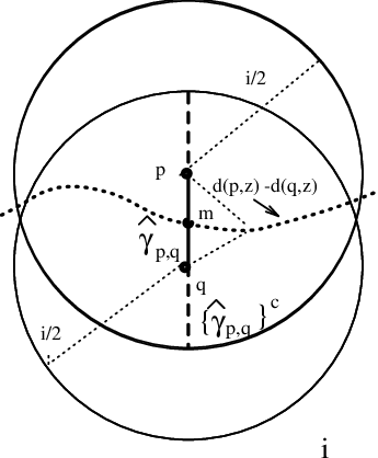
To get started it is in fact useful to consider the more general curve of the type $D_{p}-D_{q}=c$ , were $c\in\bf R$ . By the implicit function theorem when $d(D_{p}-D_{p})\neq 0$ and is defined, the solution to this equation is locally a curve $z(t)$ with $\dot{z}(t)\neq 0$ ; where $z(t)$ satisfies $d(D_{p}-D_{p})(\dot{z}(t))=0$ . In fact any such curve will parameterize a solution. It is useful to rephrase this one form business in terms of its dual object the gradient. Recall the gradient of a function $f$ is the unique vector field $\nabla f$ satisfying $<\nabla f,v>=df(v)$ for all $v$ at every point. So we may rewrite our differential relation $d(D_{p}-D_{p})(\dot{z}(t))=0$ as $<\nabla D_{p}-\nabla D_{q},\dot{z}>=0$ .

To get a grip on this differential relation it is first useful to spend a moment contemplating $\nabla D_{p}$ .

Sub-lemma 2 (The Distance Gradient Sub-lemma)

Let $d(p,q)<\frac{i}{2}$ then:

1.

In $B_{\frac{i}{2}}(p)-\{p\}$ we have $\nabla D_{p}$ is unit length with its integral curves the unit speed geodesics.
2.

In $B_{\frac{i}{2}}(p)\bigcap B_{\frac{i}{2}}(q)$ we have $\nabla D_{p}=-\nabla D_{q}$ on $\hat{\gamma}_{p,q}$ , $\nabla D_{p}=\nabla D_{q}$ on $\{\hat{\gamma}_{p,q}\}^{C}$ ; and outside $\gamma_{p,q}$ we have $\nabla D_{p}\neq c\nabla D_{q}$ for any $c\in\bf R$ .

$\bf{Proof:}$ For the first part note the distance function’s level sets are the spheres, so by Gauss’s lemma its integral curves are some re-parameterizations of geodesics from $p$ . Now observe in geodesic polar coordinates that the unit speed geodesics $\gamma$ satisfies $\dot{\gamma}=G_{\star}\left(\frac{\partial}{\partial r}\right)$ , and

<\nabla D_{p},\dot{\gamma}>=dD_{p}\left(G_{\star}\left(\frac{\partial}{\partial r}\right)\right)=G^{\star}(dD_{p})\left(\frac{\partial}{\partial r}\right)=dr\left(\frac{\partial}{\partial r}\right)=1.

So indeed the integral curve of $\nabla D_{p}$ are precisely the unit speed geodesics.

The equalities in the second part follows immediately from the first part and the fact $\gamma_{p,q}$ is a geodesic.

To prove the last piece of the second part assume at some $z\in B_{\frac{i}{2}}(p)\bigcap B_{\frac{i}{2}}(q)$ we have $\nabla D_{p}=c\nabla D_{q}$ . First note from the above we have $c=\pm 1$ . There are two cases, first we’ll deal with $c=1$ . Since the geodesics satisfy a second order O.D.E they are uniquely determined by their position and tangent vector, so when $c=1$ we have both the geodesic from $p$ and the geodesic form $q$ are the same curves. Without loss of generality $p$ is further away than $q$ and this point lies along the same minimal length geodesic (of length less than $\frac{i}{2}$ ) which connects $p$ and $q$ , i.e. $\gamma_{p,q}$ . In the case $c=-1$ we can follow the geodesic form $p$ to the point and then from the point back to $q$ forming a geodesic of length less than $i$ - which then must by lemma 12 be the unique such one, i.e. $\gamma_{p,q}$ .

q.e.d

Back to the relation $<\nabla D_{p}-\nabla D_{q},\dot{z}>=0$ . The first observation is that we can express a solution of this relation via a vector field. Using $\frac{\pi}{2}$ rotation field $\Theta$ (from section 1.1) we see that the solution to the differential relation $<\nabla D_{p}-\nabla D_{q},\dot{z}>=0$ are re-parameterizations of integral curves of the vector field $\Theta(\nabla D_{p}-\nabla D_{q})$ . Fortunately, as with $\nabla D_{p}$ , we can say quite a bit about this vector field. We are most interested in its integral curve corresponding to $D_{p}-D_{q}=0$ . Let $c_{p,q}(t)$ be the connected component of the integral curve of $\Theta(\nabla D_{p}-\nabla D_{q})$ passing through $m$ in any set of interest to us; and assume its parameterization satisfies $c_{p,q}(0)=m$ .

Lemma 35 (The Distance Difference Gradient Lemma)

Assume $d(p,q)<\frac{i}{4}$ then:

1.

In $B_{\frac{i}{4}}(p)$ we have that $c_{p,q}(t)$ is the unique component of $D_{p}-D_{q}=0$ , and $m$ is the unique point of $\gamma_{p,q}$ on $c_{p,q}(t)$ .
2.

In $B_{\frac{i}{4}}(p)\bigcup B_{\frac{i}{4}}(q)$ we have $d(c_{p,q}(t),p)$ and $d(c_{p,q}(t),q)$ strictly increase as the parameter $|t|$ increases.
3.

No geodesic from $p$ in $B_{\frac{i}{4}}(p)$ is tangent to $c_{p,q}(t)$ or cuts trough $c_{p,q}(t)$ twice on the same side of $\gamma_{p,q}(t)$ .
4.

In $B_{i}(o)-o$ it can never be the case that $\nabla D_{o}-\nabla D_{p}=c(\nabla D_{o}-\nabla D_{q})\neq 0$ at a point on $c_{p,q}(t)$ .

$\bf{Proof:}$ First for the uniqueness of $m$ : suppose a point $l\neq m$ is $\gamma_{pq}$ . Then $l$ is within $\frac{i}{4}$ of $p$ - hence $d(p,l)$ is determined by the length of the segment of $\gamma_{p,q}$ form $p$ to $l$ , similarly for $q$ (using $\frac{i}{2}$ ). Now note that as we move from $m$ toward, say, $p$ that $D_{p}$ decreases while $D_{q}$ increase - so $D_{p}-D_{q}\neq 0$ at another point of $\hat{\gamma}_{p,q}$ . When on $\{\hat{\gamma}_{p,q}\}^{c}$ say above $p$ the segment of $\gamma_{p,q}$ from $q$ to $l$ in fact covers the shorter segment from $p$ to $l$ - forcing $D_{p}-D_{q}\neq 0$ once again. So $l$ cannot satisfy $D_{p}-D_{q}=0$ , forcing $m$ to indeed be the unique point of $\gamma_{p,q}$ on $D_{p}-D_{q}=0$ .

The remainder of the first part and the second part are intimately related. To see why we first look at the component of $c_{p,q}(t)$ in $B_{\frac{i}{4}}(p)$ and note any component of $D_{p}-D_{q}=0$ would have to have a point closest to $p$ . This closest point is tangent to a sphere emanating form $p$ . The same sort of phenomena must take place for the distance function to have a critical point; namely if a point $z$ along any integral curve of $\Theta(\nabla D_{p}-\nabla D_{q})$ is a critical point of the distance function $D(p,\cdot)$ then either $\nabla D_{p}=\nabla D_{q}$ or a circle is tangent to the solution curve. In the tangent case $\Theta(\nabla D_{p}-\nabla D_{q})=c\Theta\nabla D_{p}$ , or rather $\nabla D_{p}-\nabla D_{q}=c\nabla D_{p}$ ; so both these situation we have forced the case $\nabla D_{p}=c\nabla D_{q}$ . The triangle inequality tells $B_{\frac{i}{4}}(p)\subset B_{\frac{i}{2}}(p)\bigcap B_{\frac{i}{2}}(q)$ so we may use sub-lemma 2 to note that the point where this occurs is on $\gamma_{p,q}$ ; but from above to be on $D_{p}-D_{q}=0$ and $\gamma_{p,q}$ means you must be exactly $m$ . So we have both that every component of $D_{p}-D_{q}=0$ in $B_{\frac{i}{4}}(p)$ contains $m$ , and that the distance to $p$ parameterized by $t$ can have no critical points except at $m$ (similarly for $q$ ).

For the third part note that if a geodesic cuts twice on the same side of $\gamma_{p,q}(t)$ then some other geodesic must be tangent (via the mean value theorem in geodesic polar coordinates - see the see figure 2).

So we are reduced to the tangent case. Let the point where this tangency occurs be called $z$ . This tangency implies $\Theta(\nabla D_{p}-\nabla D_{q})=c\nabla D_{p}$ , or rather $\Theta\nabla D_{q}=\Theta\nabla D_{p}-c\nabla D_{p}$ . But $\nabla D_{p}$ and $\Theta\nabla D_{p}$ are orthogonal, with $\Theta\nabla D_{p}$ also of unit length (by sub-lemma 2) - so taking norms we have $1=\sqrt{1+c^{2}}$ ; forcing $c=0$ . So at such a point $\Theta(\nabla D_{p}-\nabla D_{q})=0$ or $\nabla D_{p}=\nabla D_{q}$ . Once again using $B_{\frac{i}{4}}(p)\subset B_{\frac{i}{2}}(p)\bigcap B_{\frac{i}{2}}(q)$ the above sub-lemma applies and forces $z$ onto $\{\hat{\gamma}_{p,q}\}^{C}$ ; and now part one kicks in to eliminate this possibility of $c_{p,q}$ hitting $\{\hat{\gamma}_{p,q}\}^{C}$ .

To prove the last part we will see first if $\nabla D_{o}-\nabla D_{p}=c(\nabla D_{o}-\nabla D_{q})\neq 0$ at $z$ , then $c=1$ and $\nabla D_{p}=\nabla D_{q}$ at $z$ . This because the $\nabla D_{i}$ are all unit vectors (by sub-lemma 2 part one); and among unit vectors $v$ and $w\neq v$ the direction of $v-w$ is uniquely determined by $w$ (since we are re-parameterizing the radius one circle at located a $v$ ). Recall from the above sub-lemma that $\nabla D_{p}=\nabla D_{q}$ at $z$ implies $z\in\{\hat{\gamma}_{p,q}\}^{C}$ . As above, no point of $c_{p,q}(t)$ can be on $\{\hat{\gamma}_{p,q}\}^{C}$ , as needed.

q.e.d

The last set of issues concerns not the $c_{p,q}$ curves themselves but the home of the curves. Suppose we have three points $p$ , $q$ and $o$ on the boundary of circles of radius $r$ less than $\frac{i}{6}$ ; then using $\gamma_{p,o}$ and $\gamma_{q,o}$ we can split $B_{\frac{i}{2}}(o)$ into four cones (as in figure 3). Let the forward length cone (FLC) be the cone containing $\hat{\gamma}_{p,q}$ , the backward length cone (BLC) be the forward length cone’s mirror image (see figure 3 and the following lemma to see this is well defined). One nice thing about this cone notion is that it eliminates certain regions where the center of a small circle might have wanted to live - and it is at this point where we find the only place in the argument where using the strong convexity radius is necessary. We shall explore these facts (and clear up an issue in the introduction) with the following corollary to lemma 12 in section 1.2:

Lemma 36 (The Length Cone Lemma)

Given three points $p$ , $q$ and $o$ on the boundary of a circle of radius $r$ less than $\frac{i}{6}$ centered at $c$ :

1.

The forward length cone is well defined.
2.

The intersection of the three forward length cones is a triangle contained in $B_{\frac{i}{2}}(c)$ ; which, incidentally, can be parameterized in a way compatible with the abstract gluing to form $|K_{\{p_{1},\dots,p_{n}\}}|$ (see figure 4).
3.

The $B_{\frac{i}{2}}(c)$ is dissected by the curves $\{\gamma_{p,q},\gamma_{p,o},\gamma_{q,o}\}$ into seven regions - the unique FLC, three distinct BLCs, and the regions separating the BLCs (see in figure 4).
4.

If in addition the balls radius is less than $\tau$ , then circle’s center cannot be in any of the backward length cones, and the simplex is contained in $B_{r}(c)$ .

Proof: In the course of the this proof I use the triangle inequality in the sense of $p\in B_{a}(q)$ then $B_{b}(p)\subset B_{a+b}(q)$ . I will simply call it the triangle inequality.

First we attack well definedness of the FLC. Since the radius of the circle is less than $\frac{i}{6}$ we have by the triangle inequality $p$ and $q$ are in $B_{\frac{2i}{6}}(o)$ , and that $d(p,q)<\frac{2i}{6}$ . Now note $\hat{\gamma}_{p.q}$ is contained in $B_{\frac{3i}{6}}(o)$ - since if it left $B_{\frac{3i}{6}}(o)$ then by the triangle inequality it would be a curve from $p$ to $q$ leaving $B_{\frac{i}{6}}(p)$ and then afterwards entering $B_{\frac{i}{6}}(q)$ , so would have length greater than $\frac{2i}{6}$ ; contradicting $d(p,q)<\frac{2i}{6}$ . We would now like this geodesic segment to stays in one cone section. If it did not then it would cut a bounding geodesic, $\gamma_{o,p}$ or $\gamma_{o,q}$ , in at least two points on the cone’s boundary. Now the diameter geodesics are of length less than $i$ , so between $c_{1}$ and $c_{2}$ we now have contradictory distinct geodesics of length less than $i$ connecting them. So the cone is well defined.

To get started on the second part first simply parameterize the needed simplex. Note we may choose $\theta_{1}$ and $\theta_{2}$ such that $\gamma_{o,p}(t)=exp_{o}(tv(\theta_{1}))$ and $\gamma_{o,q}(t)=exp_{o}(tv(\theta_{2}))$ bound the FLC, and by the first argument $\hat{\gamma}_{p,q}\subset B_{\frac{3i}{6}}(o)$ so any point on $\hat{\gamma}_{p,q}$ has its shortest length geodesics from $o$ described by $exp_{o}(tv(\theta))$ with $\theta\in[\theta_{1},\theta_{2}]$ . The fact there are no double intersections of short geodesics now demonstrates that each $exp_{o}(tv(\theta))$ with $\theta\in[\theta_{1},\theta_{2}]$ hits exactly one point on $\hat{\gamma}_{p,q}$ , so we can parameterize $\hat{\gamma}_{p,q}$ as $exp_{o}(r(\theta)v(\theta))$ - with $r(\theta)$ continuous. Now we have a homeomorphism (once again since there are not double intersection between small geodesics) of the region trapped between the geodesics with the wedge $\theta\in[\theta_{1},\theta_{2}]$ and $r\leq r(\theta)$ . This wedge is clearly homeomorphic to the disk. However to parameterize the triangle we would like a parameterization which is compatible with the abstract gluing, allowing $R:|K_{\{p_{1},\dots,p_{n}\}}|\rightarrow M$ to be continuous. To accomplish this first parameterize the edges with the unit interval using a $d(p,q)$ speed parameterization of the geodesic. Now for each triangle in the surface we will map on an equilateral triangle by first mapping the boundary of our triangle to the boundary of our simplex $M$ such that the linear unit length sides are mapped onto the geodesics at a speed of $d(p,q)$ . We have just found that the image is in fact itself the boundary of a disk, so this mapping can be extended from a homeomorphism of the equilateral triangle’s boundary to a homeomorphism of the equilateral triangle onto the triangle in $M$ . So by its very construction the mapping on the boundary of the equilateral triangle is affine related to the mapping of the interval, and we indeed have the needed compatible parameterizations.

We also need for this second part that this is the same simplex for all three of the points, but by the very definition of the FLC with respect to a point being the cone section containing the opposite $\hat{\gamma}$ we have that the FLC must contain this simplex. So the simplex is in the intersection - and precisely the intersection since the respective $\gamma_{p,q}$ curves all cut their respective $B_{i}(p)$ balls in to two distinct sides - and by the triangle inequality this entire discussion is taking place in any one of the radius $i$ balls.

Lastly for the second part we need the simplex is contained in $B_{\frac{i}{2}}(c)$ ball. To see this note from above that every point, $k$ , in the simplex is on a geodesic, from say $o$ , of length less than $\frac{3i}{6}$ which hits $\hat{\gamma}_{p,q}$ . If $k$ is within $\frac{2i}{6}$ of $o$ then $k$ is with in $\frac{i}{2}$ of $c$ . If not it is within $\frac{i}{6}$ of $\hat{\gamma}_{q,o}$ . The geodesic segment $\hat{\gamma}_{q,o}$ has length less than $\frac{2i}{6}$ , so the point where the geodesic from $k$ hits $\hat{\gamma}_{q,o}$ is within $\frac{i}{6}$ of either $p$ or $q$ ; so $k$ is once again with in $\frac{3i}{6}$ of $c$ - as needed.

For the third part note that by the triangle inequality a geodesic between two points in $B_{\frac{i}{2}}(c)$ is contained in the ball must be of length less than $i$ (use the sense of the triangle inequality introducing this proof at a point were the geodesic first hits $S_{\frac{i}{2}}(c)$ ). Now extend all the geodesic segments bounding the simplex out to the boundary in $B_{\frac{i}{2}}(c)$ ; and note, having length less than $i$ these segments can intersect each other only once - at the vertices of the simplex (by part 2 above the simplex is in there). So noting the definitions of all of our objects we indeed end up decomposing $U$ into the seven components pictured in the figure.

For the final part, the fact that the simplex is contained in $B_{r}(c)$ is a trivial consequences of the $\hat{\gamma}$ curves having interior in this ball and never intersecting each other with in the ball. To handle the center’s placement, assume the contrary that the center, $c$ , is in the backward length cone with respect to say $o$ . Then take the shortest length geodesic from $c$ to $o$ and continue it through the forward length cone until it hits $\hat{\gamma}_{p,q}$ at $h$ . Note this is a geodesic of length less than $\frac{4i}{6}$ , so in particular it is the unique shortest length geodesic between these points. By assumption $p$ and $q$ are on the boundary of a disk at $c$ with radius less than $\tau$ , so by strong convexity $\hat{\gamma}_{p,q}\subset B_{r}(c)$ . In particular the shortest length geodesic to $h$ never leaves $B_{r}(c)$ , contradicting the fact it hit $o$ before $h$ . So the center must not be in the backward length cone.

q.e.d

We are finally in a position to prove the small disk uniqueness theorem form the introduction (theorem 1).

Proof of Theorem 1: As above call the points in the triple $p$ , $q$ and $o$ , and recall $\delta<min\{\frac{i}{6},\tau\}$ . The whole discussion takes place with $B_{\frac{i}{2}}(c)$ , since $d(c_{p,q}(t),c)\leq d(c_{p,q}(t),p)+d(c,p)\leq\frac{i}{3}$ . In particular the whole discussion takes place at points where we can use lemmas 35 and 3. Note a circle of radius less than $\frac{i}{6}$ passing through all three of these points corresponds to an intersection of $c_{p,q}$ and $c_{p,o}$ (by part one of lemma 35). Further note if $c_{p,q}$ and $c_{p,o}$ intersect at $z$ then so does $c_{q,o}$ , since then $d(z,p)=d(z,q)=d(z,o)$ .

At these intersections we would like that the curves must cut through each other; i.e. not be tangent. If a pair were tangent then there are two possibilities: one where neither of the tangent curves is stopped when thought of as a parameterized integral curve, and the other when one has stopped ( $\dot{c}_{p,q}=0$ ). If neither has stopped then (up to index permutation) $\Theta(\nabla D_{p}-\nabla D_{q})=c\Theta(\nabla D_{p}-\nabla D_{o})\neq 0$ , or rather $(\nabla D_{p}-\nabla D_{q})=c(\nabla D_{p}-\nabla D_{o})\neq 0$ . This case implies by lemma 2 that we are on $\{\hat{\gamma}_{q,o}\}^{C}$ . If one is stopped then (once again up to index permutation) $\nabla D_{p}-\nabla D_{q}=0$ . So by sub-lemma 2 the point of intersection is on $\{\hat{\gamma}_{p,q}\}^{C}$ . Be warned - I will refer to this same case analysis later in the argument. To finish off this impossibility argument simply note that all the curves intersect at this point so (up to index permutation) $\{\hat{\gamma}_{p,q}\}^{C}$ and $c_{p,q}$ would intersect. But by part one of lemma 35 this point must then be $m_{p,q}$ which is not on $\{\hat{\gamma}_{p,q}\}^{C}$ . So the intersection must include no tangencies.

Now suppose we had two distinct circles of radius less then $\frac{i}{6}$ passing through these triples. This non-uniqueness of circles would correspond to at least a pair of intersections of $c_{p,q}$ , $c_{p,o}$ , and $c_{q,o}$ - at $z_{1}$ and $z_{2}$ . Note without loss of generality there are no further intersections of any pair of $c$ curves between $z_{1}$ and $z_{2}$ ; since intersections occur only as triples at isolated possible distances by the above no tangency result. Hence we are forced to have a picture something very much like figure 5, at least in the sense that we have one of the curves trapped between the other two; without loss of generality assume this curve is $c_{q,o}$ .

Note $\Theta(\nabla D_{q}-\nabla D_{o})=\Theta(\nabla D_{p}-\nabla D_{o})+\Theta(\nabla D_{q}-\nabla D_{p})$ , so $\Theta(\nabla D_{p}-\nabla D_{o})$ and $\Theta(\nabla D_{q}-\nabla D_{p})$ are always on opposite sides of $\Theta(\nabla D_{p}-\nabla D_{o})$ ; in the sense that the $\nabla D_{q}-\nabla D_{o}$ component of these vectors must have opposite signs. Now since the curves must cut through each other at $z_{1}$ and $z_{2}$ and no where in between, the side of $c_{q,o}$ which $\Theta(\nabla D_{p}-\nabla D_{o})$ and $\Theta(\nabla D_{q}-\nabla D_{p})$ live on must switch roles while one moves along $c_{q,o}$ from $z_{1}$ to $z_{2}$ . In order for these roles to switch and the vectors to always be on opposite sides, we are forced (as with our no tangency result above) to have at some point along $c_{q,o}$ either $\Theta(\nabla D_{p}-\nabla D_{o})=c\Theta(\nabla D_{p}-\nabla D_{q})\neq 0$ , $\nabla D_{p}-\nabla D_{o}=0$ , or $\nabla D_{p}-\nabla D_{q}=0$ . Immediately, the last part of lemma 35 kicks in eliminating the first case.

The remaining case (up to index permutation) is were $\nabla D_{p}=\nabla D_{o}$ - which means this point lies on $\{\hat{\gamma}_{p,o}\}^{c}$ (by the sub lemma). We will be justifying each of the two pictured cases - depending on which component of $\{\hat{\gamma}_{p,o}\}^{c}$ the point lies (figure 5 and figure 6). The idea in each case is this same - we will use this condition to force one of the centers $z_{i}$ into a backward length cone with respect to either $o$ or $p$ , and then use the previous lemma to observe this is impossible.

Observe by the first and third parts of lemma 35 that $c_{q,o}(t)$ cannot be tangent to or cut twice any geodesic in the picture; and $c_{q,o}(t)$ cannot sneak around a geodesic in the picture (since the decomposition in the third part of lemma 3 has each of the geodesics heading all the way out to $S_{\frac{i}{2}}(c)$ ). So in the first case the $c_{q,o}$ is stuck to the right of $\gamma_{q,o}$ and must cross $\gamma_{p,o}$ to the right and can never cross it again. So one of the $z_{i}$ is stuck in the backwards length cone of $o$ as needed. The other case is similar to this except we must justify why we must come from above and cross into the backward length cone with respect to $p$ . This is because to come from below would mean to cut across $\gamma_{p,o}$ first to get there producing a double cut of $c_{q,o}$ by $\gamma_{p,o}$ to left of $\gamma_{q,o}$ , contradicting part 3 of lemma 35. So indeed once again we are forced into the contradictory setting of having a center in a backward length, this time with respect to $p$ .

So the points $z_{1}$ and $z_{2}$ cannot simultaneously exist - and there is no non-uniqueness among small circles.

q.e.d

References

[1] E.M. Andreev. On convex polyhedra in lobacevskii spaces. Mat.USSR Sbornik, 10:413–440, 1970.
[2] R. Phillips B. Osgood and P. Sarnak. Extremals of determinants of laplacians. J. Fun. Anal., 80:148–211, 1988.
[3] Walter Brg̈ger. Kreispackungen und triangulation. Ens. Math, 38:201–217, 1992.
[4] Yves Colin de Verdiére. Un principe variationnel pour les empilements de cercles. Prépublication de l’Institut Fourier, Grenoble, 147:0–16, 1990.
[5] B. Delaunay [Delone]. Sur la spheŕe vide. Proc. Internal. Congr. Mth., 1:695–700, 1928.
[6] M.P. do Carmo. Riemannian Geometry. Birkhauser, Boston, first (english) edition, 1991.
[7] T. Donaldson. Nonlinear elliptic boundary value problems in orlicz-sobolev spaces. J. Differential Equations, 10:507–528, 1971.
[8] S. Fortune. Voronoi diagrams and delaunay triangulations. Computing in Euclidean Geometry. Lecture Notes Ser. Comput., 1:193–233, 1992.
[9] R. S. Hamilton. The ricci flow on surfaces. Contemporary Math., 71:237–262, 1988.
[10] Z. He and O. Schramm. The $c^{\infty}$ -convergence of hexagonal disk packings to the riemann map. Acta Math., 180:219–245, 1998.
[11] Serge Lang. Real and Functional Analysis. Springer-Verlag, New York, third edition, 1993.
[12] G. Leibon. Random Delaunay Triangulations, the Thurston-Andreev Theorem and Metric Uniformization. PhD thesis, UCSD, 1999.
[13] A. Polyakov. Quantum geometry of bosonic strings. Phys. Lett. B, 103:207–210, 1981.
[14] I. Rivin. Euclidean structures on simplicial surfaces and hyperbolic volume. Ann. of Math (2), 139:553–580, 1994.
[15] I. Rivin. A characterization of ideal polyhedra in hyperbolic 3-space. Ann. of Math.(2), 143:51–70, 1996.
[16] B. Rodin and D. Sullivan. The convergence of circle packings to the riemann mapping. J. Differential Geom., 26:349–360, 1987.
[17] William P. Thurston. Three-Dimensional Geometry and Topology. The Geometry Center, University of Minnesota, draft edition, 1991.
[18] W.P. Thurston. The finite riemann mapping theorem. Unpublished talk given at the International Symposium in Celebration of the proof of the Bieberbach Conjecture (Purdue University, 1985).

Random Delaunay Triangulations, the Thurston-Andreev Theorem, and Metric Uniformization

Abstract

Acknowledgements.

Chapter 0 Introduction

Result 1

Result 2

1 A New Proof of the Gauss-Bonnet Theorem

Theorem 1

Theorem 2

Formula 1 (Euler-Delaunay-Poisson Formula)

Lemma 1 (The Small Circle Intersection Lemma)

Formula 2 (Euler-Gauss-Bonnet-Delaunay Formula)

2 Conformal Geometry and Uniformization

Formula 3

1 Discrete Uniformization

Lemma 2 (The Discrete Teleportation Lemma)

Formula 4

Observation 1

Theorem 3 (Discrete Uniformization Theorem)

Theorem 4

2 Continuous Uniformization

Lemma 3 (The Metric Teleportation Lemma)

Formula 5

Observation 2

Theorem 5 (The Metric Uniformization Theorem)

3 The Determinant of the Laplacian and Entropy

Theorem 6

3 Three-dimensional Dreams

Discrete Uniformization

From the Discrete to the Continuous

Continuous Uniformization

Chapter 1 The Discrete Uniformization Theorem

1 The Triangular Decomposition Theorem

1 Statement and Notation

Definition 1

Definition 2

Definition 3

Definition 4

Definition 5

Theorem 7

Fact 1

2 Polyhedra in the Class II

Definition 6

Definition 7

Formula 6

Note 1

Formula 7

Definition 8

3 Ideal Disk Patterns

Definition 9

Definition 10

Observation 3

4 Proof of Theorem 7

Formula 8

Definition 11

Observation 4

Lemma 4

Corollary 1

Lemma 5

2 A Warm Up Thurston-Andreev Theorem

Observation 5

Fact 2

Lemma 6

Formula 9

Theorem 8

Proposition 1

1 The Surjectivity of Ψ\Psi: the Delaunay Case

Definition 12

Lemma 7

Lemma 8

Formula 10

3 The Ideal Thurston-Andreev Theorem

1 The Statement and Reduction to Linear Algebra

Theorem 9

Note 2

Definition 13

Definition 14

Theorem 10

Fact 3

2 Proof of Theorem 10

2 Polyhedra in the Class $I$

1 The Surjectivity of $\Psi$ : the Delaunay Case