Four short stories about Toeplitz matrix calculations

Toeplitz-type equations arise in many applications in mathematics, signal processing, communications engineering, and statistics. The excellent surveys [4, 17] describe a number of applications and contain a vast list of references. The stories told in this paper are dealing with the (approximate) solution of biinfinite, infinite, and finite hermitian positive definite Toeplitz-type systems. We pay special attention to Toeplitz-type systems with certain decay properties in the sense that the entries of the matrix enjoy a certain decay rate off the diagonal. In many theoretical and practical problems this decay is of exponential or polynomial type. Toeplitz equations arising in image deblurring are one example (since often the point spread function has exponential decay - or even stronger - compact support) [19]. Kernels of integral equations also frequently show fast decay, leading to Toeplitz systems inheriting this property (see e.g. [13]). Other examples include Weyl-Heisenberg frames with exponentially or polynomially decaying window functions [25] (yielding biinfinite block-Toeplitz systems with the same behavior when computing the so-called dual window), as well as channel estimation problems in digital communications [21].

Let ${{\boldsymbol{C}}_{[-\frac{1}{2},\frac{1}{2})}}$ be the set of all $1$-periodic, continuous, real-valued functions defined on $[-\frac{1}{2},\frac{1}{2})$. For all $f\in{{\boldsymbol{C}}_{[-\frac{1}{2},\frac{1}{2})}}$, let

be the Fourier coefficients of $f$. Since $f$ is real-valued, we have $a_{k}={\overline{a}}_{-k}$.

A Laurent operator or multiplication operator associated with its defining function $f$ can be represented by the doubly infinite hermitian matrix $L=[L_{kl}]_{k,l=-\infty}^{\infty}$ with entries $L_{kl}=a_{k-l}$ for $k,l\in{\mathbb{Z}}$. For all $n\geq 1$ let $L_{n}=[(L_{n})_{kl}]_{k,l=-n+1}^{n-1}$ be the Toeplitz matrix of size $(2n-1)\times(2n-1)$ with entries $(L_{n})_{kl}=a_{k-l}$ for $k,l=-n+1,\dots,n-1$. $L_{n}$ is a finite section of the biinfinite Toeplitz matrix $L$.

A Toeplitz operator with symbol $f$ can be represented by the singly infinite matrix $T=[T_{kl}]_{k,l=0}^{\infty}$ with $T_{kl}=a_{k-l}$ for $k,l=0,1,\dots$. In this case we define $T_{n}=[(T_{n})_{kl}]_{k,l=0}^{n-1}$ as the $n\times n$ matrix with entries $(T_{n})_{kl}=a_{k-l}$ for $k,l=0,\dots,n-1$. Of course $L_{n}=T_{2n-1}$, but in what follows it will sometimes be convenient to use the notations $L_{n}$ and $T_{n}$.

As mentioned earlier, a crucial role throughout the paper plays the decay behavior of Toeplitz matrices and their inverses. Classical results of Gelfand et al. lead to a general characterization of this decay behavior for biinfinite Toeplitz matrices, see section 1. Section 2 is concerned with the approximate solution of (bi)infinite Toeplitz systems using the finite section method. Explicit error estimates are derived, showing that the approximation rate depends only on the condition number of the matrix and its decay properties. In section 3 we analyze the approximate solution of convolution equations via circulant matrices. Finally, in section 4, we derive some quantitative results for preconditioning of Toeplitz matrices by circulant embedding. Among others, we provide a theoretical explanation of numerical observations made by Nagy et al. in connection with (non)banded Toeplitz systems.

It is helpful to review a few results on the decay of inverses of certain matrices. In what follows, if not otherwise mentioned, the $2$-norm of a matrix or a vector will be denoted by $\|.\|$ without subscript.

The following theorem about the decay of the inverse of a band matrix is due to Demko, Moss, and Smith [8].

One notes that the inverse of a banded matrix is in general not banded, the type of decay changes when we switch from $A$ to $A^{-1}$ (although exponential decay is “almost as good” as bandedness). This observation suggests to look at other classes of matrices, for which the type of decay is preserved under inversion. This leads naturally to the following

The following result is due to Jaffard [16].

For finite-dimensional matrices these results (and in particular the involved constants) should be interpreted as follows. Think of the $n\times n$ matrix $A_{n}$ as a finite section of an infinite-dimensional matrix $A$. If we increase the dimension of $A_{n}$ (and thus consequently the dimension of $(A_{n})^{-1}$) we can find uniform constants independent of $n$ such the corresponding decay properties hold. This is of course not possible for arbitrary finite-dimensional invertible matrices.

Theorem 3(a) shows that the entries of $A^{-1}$ still have exponential decay, however $A^{-1}$ is in general not in the same algebra as $A$, since we may have to use a smaller exponent. However in Theorem 3(b) both, the matrix $A$ and its inverse $A^{-1}$ belong to the same algebra, the quality of decay does not change.

From this point of view Theorem 3(b) is the most striking result. The proof of Theorem 3(b) is rather delicate and lengthy. For biinfinite Toeplitz-type matrices this result can be proven much shorter (and extended to other types of decay) by using classical results of Gelfand et. al. on certain commutative Banach algebras. The following theorem is a weighted version of Wiener’s Lemma. It is implicitly contained in [10], but since it may be of independent interest we state and prove it explicitly.

Infinite Toeplitz systems arise for instance in the discretization of Wiener-Hopf integral equations or, more generally, in one-sided infinite convolution equations, see [11]. Biinfinite Toeplitz-type systems are encountered in doubly infinite (discrete) convolution equations, as well as e.g. in filter bank theory [25] or in the inverse heat problem [4]. In order to solve these problems we have to introduce a finite-dimensional model.

For let $A:{{\boldsymbol{\ell}}^{2}({\mathbb{Z}}})\mapsto{{\boldsymbol{\ell}}^{2}({\mathbb{Z}}})$ be a hermitian positive definite (hpd for short) biinfinite Toeplitz matrix given by $\{a_{k,l}\}_{k=-\infty}^{\infty}$. Let $y=\{y_{k}\}_{k=-\infty}^{\infty}\in{{\boldsymbol{\ell}}^{2}({\mathbb{Z}}})$. We want to solve the system $Ax=y$.

For $n\in{\mathbb{N}}$ and $y\in{{\boldsymbol{\ell}}^{2}({\mathbb{Z}}})$ define the orthogonal projections $P_{n}$ by

By identifying the image of $P_{n}$ with the $2n-1$-dimensional space ${\mathbb{C}}^{2n-1}$ we can express the $(2n-1)\times(2n-1)$ matrix $A_{n}$ as

where we have used that $P^{\ast}=P$. The $n$-th approximation $x^{(n)}$ to $x$ is then given by the solution of the finite-dimensional system of equations

where $y^{(n)}:=P_{n}y$.

If $A$ is a singly infinite Toeplitz matrix and $y\in{{\boldsymbol{\ell}}^{2}}({\mathbb{N}})$, we proceed analogously by defining $P_{n}$ as

This approach to approximate the solution of $Ax=y$ is usually called the finite section method, cf. [11].

The first question that arises when considering this method is “does $x^{(n)}$ converge to x?”. For the case when $A$ is not hpd this question has lead to deep mathematical results. See the book [11] and chapter 7 in [2] for more details. For the case when $A$ is hpd the answer is easy and always positive. To see this, recall that since $A$ is hpd it follows that $A_{n}$ is also hermitian positive definite, see [15]. Furthermore, $\|A_{n}\|\leq\|A\|$ and $\|(A_{n})^{-1}\|\leq\|A^{-1}\|$ for $n=1,2,\dots$. Applying the Lemma of Kantorovich [23] yields that $(A_{n})^{-1}$ converges strongly to $A^{-1}$ for ${n\rightarrow\infty}$, i.e., $x^{(n)}$ converges to $x$ in the ${{\boldsymbol{\ell}}^{2}}$-norm for any $y\in{{\boldsymbol{\ell}}^{2}({\mathbb{Z}}})$ (or for any $y\in{{\boldsymbol{\ell}}^{2}}({\mathbb{N}})$ if $A$ is singly infinite).

An important aspect for applications is if we can give an estimate on how fast $x^{(n)}$ converges to $x$. It will be shown that the rate of approximation depends on the decay behavior and the condition number of the matrix.

The proof of Theorem 6 is essentially based on the fact that under appropriate decay conditions on $L$ and $y$ (resp. $L_{n}$ and $y^{(n)}$) $L^{-1}$ and $L_{n}^{-1}y^{(n)}$ have similar decay properties. Thus, if one can show that $L_{n}^{-1}$ has the same decay properties as $L^{-1}$ one can use Theorem 4 in order to generalize Theorem 6 to various other decay conditions. This may however not always lead to simple and closed-form expressions for $\|(L_{n}-L)L_{n}^{-1}y^{(n)}\|$, therefore I have restricted myself to the most frequently encountered decay properties.

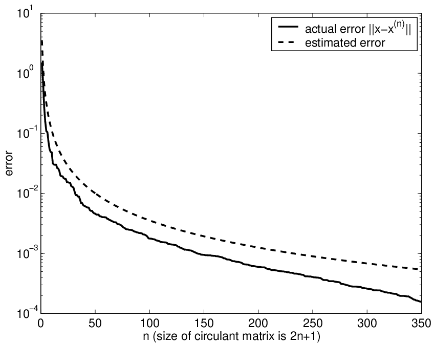
Example 1: We illustrate Theorem 6 by a numerical example. We consider $Lx=y$, where $L$ is the biinfinite Toeplitz matrix with entries $a_{k}=(1+|k|)^{-s},k\in{\mathbb{Z}}$ for $s=2$ and $y$ consists of random entries having the same polynomial decay rate as the entries $a_{k}$. To compare the error $\|x-x^{(n)}\|$ with the error estimate (11) we would need the true solution $x$. Since the solution of this biinfinite system cannot be computed analytically we compute the “true” solution of $Lx=y$ by solving $L_{n_{0}}x^{(n_{0})}=y^{(n_{0})}$ for very large $n_{0}$ (we choose $n_{0}=32768$). Using (12) and (18) we can estimate that in the worst case $\|x-x^{(32768)}\|\approx 10^{-6}$, so that $x^{(32768)}$ can mimick the true solution with sufficiently high accuracy for this experiment.

Then we approximate this solution by the finite section method as in Theorem 6 for $n=0,\dots,350$ and compute for each $n$ the error $\|x-x^{(n)}\|$ as well as the error estimate in (11). Note that an explicit expression for the constant $c_{1}$ in (11) is not known, we only know that it depends on the condition number of $L$. In this example we use $c_{1}=\mbox{cond\/}(L)$ (a different example may require a different choice). The result, illustrated in Figure 1, shows that the asymptotic behavior of the error rate is well estimated by the given error bound.

It is well-known that the product of two Laurent operators and the inverse of a Laurent operator (if it exists) is again a Laurent operator. This is of course not true for singly infinite or finite Toeplitz matrices (and this is one of the reasons which makes the “Toeplitz business” so interesting). Hence one may argue that the “canonical” finite-dimensional analogue of Laurent operators are not Toeplitz matrices but circulant matrices, since they also form an algebra. Thus for a given biinfinite hermitian Toeplitz matrix $L$ with entries $L_{kl}=a_{k-l}$ we define the hermitian circulant matrix $C_{n}$ of size $(2n-1)\times(2n-1)$ by

We also say that $C_{n}$ is generated by $\{a_{k}\}_{k=-n+1}^{n-1}$.

We can do even a little better and estimate how well the extrema of the defining function of $L$ are approximated by the extreme eigenvalues of $C_{n}$.

It is obvious that decay properties for circulant matrices cannot be defined in the same way as for non-circulant matrices. Hence, by stating that $C_{m}$ has, say, exponentially decaying entries, we mean that the generating sequence $\{a_{k}\}_{k=-m+1}^{m-1}$ satisfies $|a_{k}|\leq ce^{-\gamma|k|}$, in which case the entries of $C_{m}$ will decay exponentially off the corners of the matrix (instead of off the diagonal). In analogy to the theorems in section 1 it is natural to ask if the inverse of $C_{m}$ also inherits these decay properties. The following theorem shows that at least for $m$ sufficiently large this is the case. The entries of $C_{m}^{-1}$ uniformly approximate the entries of $L^{-1}$ with an error rate depends on the decay properties and the condition number of $L$.

References

- [1] A. Beurling, Sur les intégrales de Fourier absolument convergentes et leur application à une transformation fonctionelle, in Ninth Scandinavian Math. Congress, Helsingfors, 1938, pp. 345–366.
- [2] A. Böttcher and B. Silbermann, Analysis of Toeplitz operators, Springer-Verlag, Berlin, 1990.
- [3] R. Chan, Circulant preconditioners for hermitian Toeplitz systems, SIAM J. Matrix Anal. Appl., 10 (1989), pp. 542–550.
- [4] R. Chan and M. Ng, Conjugate gradient methods for Toeplitz systems, SIAM Review, 38 (1996), pp. 427–482.
- [5] R. Chan and G. Strang, Toeplitz equations by conjugate gradients with circulant preconditioner, SIAM J. Sci. Stat. Comput., 10 (1989), pp. 104–119.
- [6] R. H. Chan and M. Ng, Toeplitz preconditioners for Hermitian Toeplitz systems, Linear Algebra Appl., 190 (1993), pp. 181–208.
- [7] P. Davis, Circulant Matrices, John Wiley, 1979.
- [8] S. Demko, W. Moss, and P. Smith, Decay rates for inverses of band matrices, Math. Comp., 43 (1984), pp. 491–499.
- [9] Y. Domar, Harmonic analysis based on certain commutative Banach algebras, Acta Math., 96 (1956), pp. 1–66.
- [10] I. Gelfand, D. Raikov, and G. Shilov, Commutative normed rings, Chelsea Publishing Co., New York, 1964. Translated from the Russian.
- [11] I. Gohberg and I. Fel’dman, Convolution equations and projection methods for their solution, American Mathematical Society, Providence, R.I., 1974. Translated from the Russian by F. M. Goldware, Translations of Mathematical Monographs, Vol. 41.
- [12] I. Gohberg, S. Goldberg, and M. A. Kaashoek, Classes of linear operators. Vol. II, vol. 63 of Operator Theory: Advances and Applications, Birkhäuser Verlag, Basel, 1993.
- [13] I. Gohberg, M. Hanke, and I. Koltracht, Fast preconditioned conjugate gradient algorithms for Wiener-Hopf integral equations, SIAM J. Numer. Anal., 31 (1994), pp. 429–443.
- [14] M. Hanke and J. G. Nagy, Toeplitz approximate inverse preconditioner for banded Toeplitz matrices, Numer. Algorithms, 7 (1994), pp. 183–199.
- [15] R. Horn and C. Johnson, Topics in matrix analysis, Cambridge University Press, Cambridge, 1994.
- [16] S. Jaffard, Propriétés des matrices “bien localisées” près de leur diagonale et quelques applications, Ann. Inst. H. Poincaré Anal. Non Linéaire, 7 (1990), pp. 461–476.
- [17] T. Kailath and A. H. Sayed, Displacement structure: theory and applications, SIAM Rev., 37 (1995), pp. 297–386.
- [18] S. Levin, Asymptotic properties of Toeplitz matrices, PhD thesis, The Weizmann Institute, Rehovot, Israel, 1980.
- [19] J. Nagy, R. Plemmons, and T. Torgersen, Iterative image restoration using approximate inverse preconditioning, IEEE Trans. Image Processing, 15 (1996), pp. 1151–1162.
- [20] M. K. Ng, R. H. Chan, and W.-C. Tang, A fast algorithm for deblurring models with Neumann boundary conditions, SIAM J. Sci. Comput., 21 (1999), pp. 851–866 (electronic).
- [21] J. G. Proakis, Digital Communications, McGraw-Hill, New York, 3rd ed., 1995.
- [22] H. Reiter, Classical Harmonic Analysis and Locally Compact Abelian Groups, Oxford University Press, 1968.
- [23] R. Richtmyer and K. Morton, Difference Methods for Initial-Value Problems, Krieger Publishing Company, Malabar, Florida, 1994.
- [24] G. Steidl, Personal communication, 2000.
- [25] T. Strohmer, Rates of convergence for the approximation of dual shift-invariant systems in , J. Four. Anal. Appl., 5 (2000), pp. 599–615.