Recall that, in the most general sense, a link invariant is a map from the set of equivalence classes of links under isotopy to another set $G$. We will need to have some additional structure on $G$. For our purposes, $G$ will be the field of complex numbers $\mathbb{C}$. In this theory, it is also convenient to look at invariants of regular isotopy (i.e. links with framing), rather than just isotopy. So we will not allow the first Reidemeister move. We first note that we can extend any link invariant to an invariant of singular links, where a singular link is an immersion of several copies of $S^{1}$ into 3-space which is an embedding except for a finite number of isolated double points. Given a link invariant $v$, we extend it via the relation:

An invariant $v$ of singular links is then said to be of finite type, if there is an integer $d$ such that $v$ is zero on any link with more than $d$ double points. $v$ is then said to be of type $d$. We denote by $V_{d}$ the vector space over $\mathbb{C}$ generated by $\mathbb{C}$-valued finite type invariants of type $d$. We can completely understand the space of $\mathbb{C}$-valued finite type invariants by understanding all of the quotient spaces $V_{d}/V_{d-1}$.

The idea of link homotopy (or just homotopy) was introduced by Milnor [13]. Two links are homotopic if one can be transformed into the other through a sequence of ambient isotopies of $S^{3}$ and crossing changes of a component with itself (but not crossing changes of different components). Habegger and Lin [6] succeeded in classifying links up to homotopy. We construct a theory of finite type invariants in exactly the same way as before; the difference is that the invariants are trivial when evaluated on a link with a singularity in which a component intersects itself. In this case, the two ”resolutions” of the singular point are homotopically equivalent, so the value of a homotopy invariant on their difference is zero. We will denote the vector space of type $d$ link homotopy invariants by $V_{d}^{h}$.

We will denote the vector space of type $d$ link concordance invariants by $V_{d}^{c}$.

It is a marvelous fact that the vector spaces $V_{d}^{*}/V_{d-1}^{*}$ can be given relatively simple combinatorial descriptions in terms of unitrivalent diagrams. These are spaces of unitrivalent graphs (with colored endpoints and oriented vertices) with various relations imposed upon them. That these descriptions are isomorphic to the original vector spaces is largely due to Kontsevich and his integral (see [5] for an excellent exposition of the Kontsevich integral). The description of the space for link homotopy was developed by Bar-Natan and others [1, 3]. The modification for concordance was found by Habegger and Masbaum [7]. For a more detailed development, see [10, 11].

Consider a diagram $D\in B^{h}(k)$. Each component of $D$ is a tree diagram with at most one endpoint of each color. Since a unitrivalent tree with $n$ endpoints has $2n-2$ vertices, and hence degree $n-1$, $D$ cannot have any components of degree greater than $k-1$. Notation: Before we continue, we will introduce a bit of notation which will be useful in this section. Given a unitrivalent diagram $D$, we define $m(D;i,j)$ to be the number of components of $D$ which are simply line segments with ends colored $i$ and $j$, as shown below:

We call these components struts. Recall the following (correct) results from [10]. We include the proofs for completeness, and as a warm up for the more complicated proof in Section 2.2:

Proof: $C$ has one endpoint of each color $1,2,...,k$. Without loss of generality, we may assume that $C$ has a branch as shown, where $\bar{C}$ denotes the remainder of $C$:

We are going to apply the link relation with the color 1. Let $\{C_{1},...,C_{n}\}$ be the components of $D$ with an endpoint colored 1. So, ignoring the other components of $D$, we have the diagrams of Figure 3 (where $\bar{C_{i}}$ denotes all of $C_{i}$ except for the endpoint colored 1).

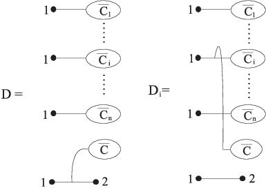The link relation then implies that $D+\sum{D_{i}}=0$. If $C_{i}$ is just a line segment with endpoints colored 1 and 2, then $D_{i}=D$. Otherwise, $\bar{C_{i}}$ will have an endpoint of some color $j\in{3,...,k}$. In this case, since $\bar{C}$ has an endpoint of each color 3,…,$k$, including $j$, $D_{i}$ will have a component with two endpoints colored $j$, and hence be trivial in $B^{h}$. Therefore, we find that $D+m(D;1,2)D=0$ where $m(D;1,2)\geq 0$. We can divide both sides by $1+m(D;1,2)$ (since we are working over a field of characteristic 0) to conclude that $D=0$. $\Box$

Proof: Without loss of generality, $C$ has endpoints colored $1,2,...,k-1$. We will prove the lemma by inducting on $m(D;1,k)$; inducting among the set of diagrams having a component with endpoints colored $1,2,...,k-1$. As in the previous theorem, we may assume that $C$ has a branch as shown:

And conclude that $D+\sum{D_{i}}=0$, where the $D_{i}$ are defined as before. Since $\bar{C}$ contains endpoints of all colors except 1, 2, and $k$, $D_{i}$ has two endpoints of the same color (and hence is trivial) unless $C_{i}$ has one of the following 3 forms (as in Theorem 2):

In the first case, $D_{i}=D$; and in the second case, $D_{i}=D^{\prime}$, where $D^{\prime}$ is the same as $D$ except that:

• •

  $C$ is replaced by a component $C^{\prime}$ identical to it except that the endpoint colored 2 in $C$ is colored $k$ in $C^{\prime}$ (so $\bar{C^{\prime}}=\bar{C}$).

• •

  A line segment with endpoints colored 1 and $k$ has been replaced by a line segment with endpoints colored 1 and 2. In other words, $m(D^{\prime};1,2)=m(D;1,2)+1$ and $m(D^{\prime};1,k)=m(D;1,k)-1$.

In the third case, $D_{i}$ has a component of degree $k-1$, and so is trivial by the previous theorem. Therefore, we find that $D+m(D;1,2)D+m(D;1,k)D^{\prime}=0$. If $m(D;1,k)=0$ we conclude, as before, that $D$ is trivial modulo the link relation, which proves the base case of our induction.

For the inductive step, we use the IHX relation on $C^{\prime}$ to decompose $D^{\prime}=\sum_{i\neq 1,2,k}{\pm D_{i}^{\prime}}$, where $D_{i}^{\prime}$ is the same as $D^{\prime}$ except that $C^{\prime}$ has been replaced by a component $C_{i}^{\prime}$ with endpoints of the same colors (although arranged differently), and a branch as shown:

(The decomposition is simply a matter of letting the endpoint colored $k$ “travel” the tree - see Figure 4 for an example.) In particular, $m(D_{i}^{\prime};a,b)=m(D^{\prime};a,b)$ for all colors $a$ and $b$.

We now apply the link relation to $D_{i}^{\prime}$ using color $i$ (and component $C_{i}^{\prime}$). In this case, the only other components which matter (modulo trivial diagrams) are ones which look like one of the following:

As before, the first case gives $D_{i}^{\prime}$ again, the third case is trivial by Theorem 2, and the second case gives a diagram $D_{i}^{\prime\prime}$ such that:

• •

  $C_{i}^{\prime}$ is replaced by a component $C_{i}^{\prime\prime}$ identical to it except that the endpoint colored $k$ in $C_{i}^{\prime}$ is colored 2 in $C_{i}^{\prime\prime}$ (so $\bar{C_{i}^{\prime\prime}}=\bar{C_{i}^{\prime}}$).

• •

  A line segment with endpoints colored $i$ and 2 has been replaced by a line segment with endpoints colored $i$ and $k$. In other words, $m(D_{i}^{\prime\prime};i,k)=m(D_{i}^{\prime};i,k)+1$ and $m(D_{i}^{\prime\prime};i,2)=m(D_{i}^{\prime};i,2)-1$.

Otherwise, $D_{i}^{\prime\prime}$ is the same as $D_{i}^{\prime}$; in particular, $m(D_{i}^{\prime\prime};1,k)=m(D_{i}^{\prime};1,k)=m(D^{\prime};1,k)=m(D;1,k)-1$. Then the link relation tells us that $D_{i}^{\prime}+m(D^{\prime};i,k)D_{i}^{\prime}+m(D^{\prime};2,i)D_{i}^{\prime\prime}=0$. Since $D_{i}^{\prime\prime}$ has a component of degree $k-2$ with endpoints colored $1,...,k-1$ (namely, $C_{i}^{\prime\prime}$), the inductive hypothesis implies that $D_{i}^{\prime\prime}$ is trivial. Therefore, $(1+m(D^{\prime};i,k))D_{i}^{\prime}=0$, so $D_{i}^{\prime}$ is trivial in $B^{h}(k)$. This is true for every $i$, so it immediately follows that $D^{\prime}$, and hence $D$, are also trivial in $B^{h}(k)$. $\Box$

So the largest possible degree of a component of a diagram in $B^{h}(k)$ is $k-3$ (if $k\geq 4$). In particular, this means that if $k$ is 3 or 4, then the largest possible degree of a component of a diagram in $B^{h}(k)$ is 1. It is well-known that the pairwise linking numbers are the only type 1 link homotopy invariants, and are dual to struts via the isomorphism of Theorem 1. Their products are dual to disjoint unions of struts. So we have as a corollary:

The obvious question is whether this result will generalize to links with more components. In the next section we will show, by a rather involved combinatorial argument, that it does extend to links with five components. However, in Section 3 we will show that it fails for links with more than 8 components.

Remark: The error in [10] (replicated in [11]) was in the attempt to generalize the result to all $k$. On page 785 of [10], line 15, the possibility that $c=a$ was neglected. This adds another term to the sum, which ends up cancelling everything out. This was pointed out by Alexander Merkov [12].

In this section we consider the $B^{h}(5)$. We know that no diagram in this space has a component of degree 3 or more. So the question is whether a diagram can have a component of degree 2. Any such component will be a ”Y-component” - i.e. a graph with three (colored) univalent vertices connected to a single trivalent vertex.

Proof: This proof is significantly more delicate than that for Theorem 3, involving an extra level of induction. Without loss of generality, $C$ has endpoints colored $1,2,3$.

Our first induction is on $m(D;1,4)+m(D;1,5)$; inducting among the set of diagrams having a component with endpoints colored $1,2,3$. We will begin by proving the base case of this induction.

Let $\{C_{1},...,C_{n}\}$ be the other components of $D$ with an endpoint colored 1. Then we apply the link relation as in Figure 3. We will apply the relation along the color 1, fixing the color 3. This means that $\bar{C}$ (in Figure 3) is just a single univalent vertex, colored 3. This will be successively attached to the components $C_{i}$ to form the diagrams $D_{i}$ (in the figure $\bar{C_{i}}$ denotes all of $C_{i}$ except for the endpoint colored 1). We will refer to this operation as ”expanding along 1, fixing 3.”

So then $D+\sum{D_{i}}=0$. $D_{i}$ has two endpoints of the same color unless $C_{i}$ has one of the following 4 forms:

In the first case, $D_{i}=D$. In the fourth case, $D_{i}$ has a component of degree 3, and so is trivial by Theorem 3.

In the second case, $D_{i}=D_{4}$, where $D_{4}$ is the same as $D$ except that:

• •

  $C$ is replaced by a component $C^{\prime}$ identical to it except that the endpoint colored 2 in $C$ is colored 4 in $C^{\prime}$.

  $$C^{\prime}:\ \ \begin{matrix}3\\ |\\ |\\ 1-----4\end{matrix}$$

• •

  A strut with endpoints colored 1 and 4 has been replaced by a strut with endpoints colored 1 and 2. In other words, $m(D^{\prime};1,2)=m(D;1,2)+1$ and $m(D^{\prime};1,4)=m(D;1,4)-1$.

Notation: For the remainder of this proof, we will represent diagrams by giving the changes made from $D$. We will draw the new component of degree 2 which has replaced $C$ (we will see that for all of our diagrams, any other components of degree 2 remain unchanged). Although the total number of struts is always preserved, some struts have been replaced by others. We represent a strut by the (unordered) pair of the colors of its endpoints, and use an arrow to show how the struts have been traded. For example, we will represent $D_{4}$ as follows:

Finally, in the third case, $D_{i}=D_{5}$, which is defined similarly to $D_{4}$.

Therefore, we find that $D+m(D;1,2)D+m(D;1,4)D_{4}+m(D;1,5)D_{5}=0$. If $m(D;1,4)+m(D;1,5)=0$, then we conclude $D+m(D;1,2)D=0$ (since $m(D;i,j)\geq 0$). Since $m(D;1,2)\geq 0$, we can divide by $1+m(D;1,2)$ to conclude $D=0$, which proves the base case of our first induction.

Henceforth, for convenience, we will let $m(i,j)=m(D;i,j)$.

We will now assume the inductive hypothesis that any diagram $E\in B^{h}(5)$ with a component of degree 2 with endpoints colored 1, 2 and 3, and such that $m(E;1,4)+m(E;1,5)<m(1,4)+m(1,5)$, is trivial. Our inductive step consists of using this hypothesis to prove that $D_{4}$ and $D_{5}$ are trivial. This will immediately imply that $D+m(1,2)D=0$, and hence that $D=0$.

We will prove that $D_{4}$ is trivial. The proof that $D_{5}$ is trivial is very similar. This proof involves a second induction. We will be looking at diagrams which do not have a component with endpoints colored 1, 2 and 3, so are not directly trivial by the (first) inductive hypothesis. However, we will find that (modulo the inductive hypothesis), we can effectively ”swap” struts in these diagrams so that the number of struts with certain colors on their endpoints always decreases. Since there are only a finite number of such struts, the supply eventually disappears, and we are able to conclude that the diagrams are trivial.

We begin with $D_{4}$. We expand along 3, fixing 1.

$D_{42}$ has a component of degree 2 with endpoints colored 1, 2, and 3. Also, $m(D_{42};1,4)+m(D_{42};1,5)=(m(1,4)-1)+m(1,5)=m(1,4)+m(1,5)-1$. So by the inductive hypothesis, $D_{42}=0$. Therefore:

Consider $D_{45}$. We expand along 3, fixing 5.

Therefore:

Neither of the new diagrams are trivial inductively, so we will need to analyze both of them. First, we consider $D_{452}$. We will show that, modulo the inductive hypothesis, we can swap a strut (3,5) (i.e. a strut with endpoints colored 3 and 5) for a strut (3,4), while simultaneously swapping a strut (2,4) for a strut (2,5). We begin by expanding along 2, fixing 3.

By the inductive hypothesis, $D_{4521}=0$. Therefore:

Now consider $D_{4524}$. We expand along 3, fixing 2.

By the inductive hypothesis, $D_{45241}=0$. Therefore:

Combining this with the result of the previous step, we have:

Notice that the component of degree 2 in $D_{45245}$ is the same as that in $D_{452}$, so we could start the whole procedure again. Also notice that we have swapped the struts as we wanted. Inductively, we can see that:

Eventually, $n>m(3,5)$, so $D_{452}=0$. This means that:

Now we examine $D_{454}$. We expand along 4, fixing 3.

Notice that $D_{4542}$ has a degree 2 component which is the same, up to sign, as $D_{4524}$. So, by using the same kind of argument used for $D_{452}$, we can show that $D_{4542}=0$ (we will look at the diagrams $D_{4542(54)^{n}}$). So:

Therefore, we can express $D_{4}$ in terms of $D_{4541}$:

Notice that we have swapped a strut (1,4) for a strut (4,5), and a strut (3,5) for a strut (3,4). Since $D_{4541}$ has the same degree 2 component (up to sign) as $D_{4}$, we can repeat the same sequence of operations. Inductively, we will find that:

Eventually, $n>m(1,4)$, so $D_{4}=0$.

By a similar argument, $D_{5}$ will equal 0, so we can conclude that $D+m(1,2)D=0$. Therefore, $D=0$, which completes the proof. $\Box$

It appears to be difficult to extend the proof of Theorem 4 to $B^{h}(6)$. In this case, the IHX relation comes into play, and it is not clear that one can decrease $m(1,4)+m(1,5)$ monotonically.

Unlike for homotopy, there is no a priori limit on the size of the components of diagrams in $B^{c}(k)$. However, we are able to prove some non-existence results for small values of $k$. The proofs of the following results can be found in [11]:

As with homotopy, it seems difficult to extend the methods used to prove Theorem 5 to higher values of $k$. The attempt in [11] fell prey to the same error as in [10] (see the Remark in Section 2.1).

Remark: If we allow the first Reidemeister move, we can prove that $B^{c}(1)$ (with the new relation) is trivial, confirming a result of [14] that the Arf invariant (which is $\mathbb{Z}_{2}$-valued) is the only finite type knot concordance invariant.

References

- [1] Bar-Natan, D.: On the Vassiliev Knot Invariants, Topology 34, No. 2, 1995, pp. 423-472
- [2] Bar-Natan, D.: Vassiliev Homotopy String Link Invariants, J. of Knot Theory and its Ramifications 4, No. 1, 1995, pp. 13-32
- [3] Bar-Natan, D., Garoufalidis, S., Rozansky, L. and Thurston, D.: The Aarhus Integral of Rational Homology 3-Spheres II: Invariance and Universality, preprint, January 1998, arXiv:math.QA/9808013
- [4] Birman, J. and Lin, X.S.: Knot polynomials and Vassiliev’s Invariants, Invent. Math. 111, 1993, pp. 225-270
- [5] Chmutov, S. and Duzhin, S.: The Kontsevich Integral, preprint, October 1999, available from ftp.botik.ur/pub/local/zmr/ki.ps.gz
- [6] Habegger, N. and Lin, X.S.: The Classification of Links up to Link-Homotopy, J. of the Amer. Math. Soc. 3, No. 2, 1990, pp. 389-419
- [7] Habegger, N. and Masbaum, G.: The Kontsevich Integral and Milnor’s Invariants, preprint, April 1997
- [8] Kneissler, J. The number of primitive Vassiliev invariants up to degree 12, preprint, 1997, arXiv:q-alg/9706022
- [9] Le, T. and Murakami, J.: The Universal Vassiliev-Kontsevich Invariant for Framed Oriented Links, Compositio Math 102, 1996, pp. 41-64, arXiv:hep-th/9401016
- [10] Mellor, B.: Finite Type Link Homotopy Invariants, J. of Knot Theory and its Ramifications 8, No. 6, 1999, pp. 773-787, arXiv:math.GT/9807162
- [11] Mellor, B.: Finite Type Link Concordance Invariants, J. of Knot Theory and its Ramifications 9, No. 3, 2000, pp. 367-385, arXiv:math.GT/9904169
- [12] Merkov, A.: private communication, March 2000
- [13] Milnor, J.: Link groups, Ann. of Math. 59, 1954, pp. 177-195
- [14] Ng, K.: Groups of Ribbon Knots, Topology 37, No. 2, 1998, pp. 441-458, arXiv:q-alg/9502017
- [15] Stanford, T.: Finite-Type Invariants of Knots, Links, and Graphs, Topology 35, No. 4, 1996, pp. 1027-1050