On the Jones polynomials of
checkerboard colorable virtual knots

In 1996, L. H. Kauffman introduced the notion of a virtual knot, which is motivated by study of knots in a thickened surface and abstract Gauss codes, cf. [8, 9]. M. Goussarov, M. Polyak, and O. Viro [1] proved that the natural map from the category of classical knots to the category of virtual knots is injective; namely, if two classical knot diagrams are equivalent as virtual knots, then they are equivalent as classical knots. Thus, virtual knot theory is a generalization of knot theory. It is also found in their paper [1] that the notion of a virtual knot is helpful to study of finite type invariants.

Kauffman defined the Jones polynomial of a virtual knot, which is also called the normalized bracket polynomial or the $f$-polynomial (cf. [9]). In this paper, according to [9], we call it the $f$-polynomial instead of the Jones polynomial, since the definition is different from Jones’ in [2, 3]. Finite type invariants derived from the $f$-polynomials are studied in [9], and it is proved that a certain property of them (Corollary 14 of [9]) is hold in the category of virtual knots.

The $f$-polynomial (Jones polynomial) of a virtual link is quite different from $f$-polynomials of classical links. For a Laurent polynomial $f$ on valuable $A$, we denote by ${\rm EXP}(f)$ the set of integers appearing as exponents of $f$. For example, if $f=3A^{-2}+6A-7A^{5}$, then ${\rm EXP}(f)=\{-2,1,5\}$. It is well-known that for a classical link $L$ with $n$ components, the $f$-polynomial satisfies that ${\rm EXP}(f)\subset 4{\bf Z}$ if $n$ is odd, and ${\rm EXP}(f)\subset 4{\bf Z}+2$ if $n$ is even. However, this is not true for a virtual knot/link in general. In this paper we introduce the notion of checkerboard coloring of a virtual link diagram as a generalization of checkerboard coloring of a classical link diagram.

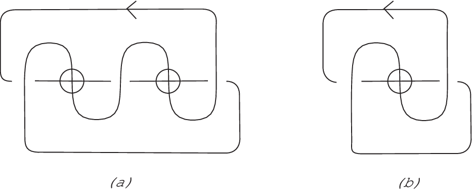
For example the virtual knot diagram illustrated in Figure 1 (a) admits a checkerboard coloring and the $f$-polynomial is $A^{4}+A^{12}-A^{16}$. So ${\rm EXP}(f)\subset 4{\bf Z}$. On the other hand, virtual knot diagram illustrated in Figure 1 (b) does not admit a checkerboard coloring and the $f$-polynomial is $-A^{10}+A^{6}+A^{4}$. Theorem 1 implies that this diagram is never equivalent to a diagram that admits a checkerboard coloring.

If a virtual link diagram is alternating (the definition is given later), then the diagram admits a checkerboard coloring. Thus we have the following.

By this corollary, we see that the virtual knot represented by Figure 1 (b) is not equivalent to an alternating diagram.

A virtual link diagram is a closed oriented 1-manifold generically immersed in ${\bf R}^{2}$ such that each double point has information of a crossing (as in classical knot theory) or a virtual crossing which is indicated by a small circle around the double point. The moves of virtual link diagrams illustrated in Figure 2 are called generalized Reidemeister moves. Two virtual link diagrams are said to be equivalent if they are related by a finite sequence of generalized Reidemeister moves. We call the equivalence class of a virtual link diagram a virtual link.

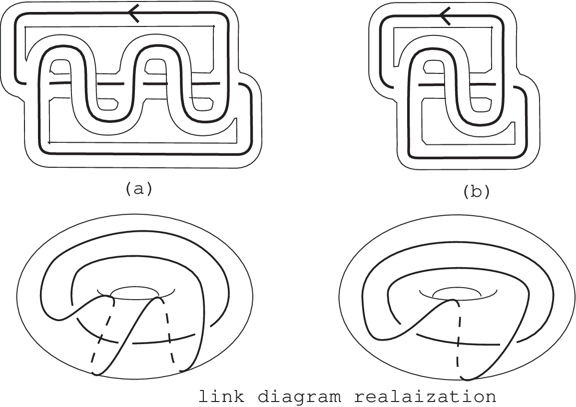
A pair $P=(\Sigma,D)$ of a compact oriented surface $\Sigma$ and a link diagram $D$ in $\Sigma$ is called an abstract link diagram (ALD) if $|D|$ is a deformation retract of $\Sigma$, where $|D|$ is a graph obtained from $D$ by replacing each real/virtual crossing point with a vertex. For an ALD, $P=(\Sigma,D)$, if there is an orientation preserving embedding $f:\Sigma\rightarrow F$ into a closed oriented surface $F$, $f(D)$ is a link diagram in $F$. We call it a link diagram realization of $P$ in $F$. In Figure 3, we show two abstract link diagrams and their link diagram realizations. Two ALDs $P=(\Sigma,D)$, $P^{\prime}=(\Sigma^{\prime},D^{\prime})$ are related by an abstract Reidemeister move (of type I, II or III) if there is a closed oriented surface $F$ and link diagram realizations of $P$ and $P^{\prime}$ in $F$ which are related by a Reidemeister move (of type I, II or III) in $F$. Two ALDs are equivalent if they are related by a finite sequence of abstract Reidemeister moves. We call the equivalence class of an ALD an abstract link.

In [6] a map

was defined. The idea of this map is illustrated in Figure 4. Refer to [6] for the definition. We call $\phi(D)$ an ALD associated with a virtual link diagram $D$. The ALDs in Figure 3 (a) and (b) are ALDs associated with the virtual link diagrams in Figure 1 (a) and (b) respectively.

Let $P=(\Sigma,D)$ be a pair of a compact oriented surface $\Sigma$ and a link diagram $D$ in $\Sigma$. A checkerboard coloring is a coloring of the all components of $\Sigma-|D|$ by two colors, say black and white, such that two components of $\Sigma-|D|$ which are adjacent by an edge of $D$ have always distinct colors.

We say that a virtual link diagram admits a checkerboard coloring or it is checkerboard colorable if the associated ALD admits a checkerboard coloring.

An ALD, $P=(\Sigma,D)$, is said to be unoriented if the diagram $D$ is unoriented. There is a unique map

satisfying the following rules.

1. (i)

   $<T>_{F}=1$ where $T$ is a one-component trivial ALD,

2. (ii)

   $<T\amalg D>=(-A^{2}-A^{-2})<D>$ if $D$ is not empty, where $\amalg$ means the disjoint union, and

3. (iii)

   $<\vbox to15.0pt{\epsfbox{crsald.eps}}>=A<\vbox to12.0pt{\epsfbox{crsBald.eps}}>+A^{-1}<\vbox to15.0pt{\epsfbox{crsAald.eps}}>$.

Then $<\quad>$ is an invariant under abstract Reidemeister moves II and III. We call it the Kauffman bracket polynomial of ALD, cf. [4].

Let $P=(\Sigma,D)$ be an unoriented ALD. Replacing the neighborhood of a double point as in Figure 5, we have another unoriented ALD. We call it an unoriented ALD obtained from $D$ by doing an A-splice  or B-splice  at the crossing point. An unoriented trivial ALD obtained from $P$ by doing an A-splice or B-splice at each crossing point is said to be a state  of $P$. From the definition of $<\quad>$, we see

where $S$ runs over all of states of $D$, $\natural(S)$ is the number of A-splice minus that of B-splice used for obtaining $S$ and $\sharp(S)$ is the number of components of $S$.

For an ALD, $P=(\Sigma,D)$, the writhe $\omega(P)$ is defined by the number of positive crossings minus the number of negative crossings. Then we define the normalized bracket polynomial or the $f$-polynomial of $P$ by

By normalizing by $(-A^{3})^{-\omega(P)}$, this value is preserved under abstract Reidemeister moves of type I. Thus this is an invariant of an abstract link. This invariant was defined in [4], where it is called the Jones polynomial of $P$. It should be noted that the bijection $\Phi$ preserves the $f$-polynomial.

Let $p$ be a crossing point of an ALD, $P=(\Sigma,D)$. Let $P_{0}=(\Sigma_{0},D_{0})$ and $P_{\infty}=(\Sigma_{\infty},D_{\infty})$ be ALDs obtained from $P$ by splicing at $p$ orientation coherently and orientation incoherently, respectively. Note that $D_{\infty}$ does not inherit an orientation from $D$. The crossing point $p$ is either (i) a self-intersection of an immersed loop of $D$ or (ii) an intersection of two immersed loops. Let $\alpha$ and $\alpha^{\prime}$ be the immersed open arcs obtained from the loop (in case (i)) or from the two loops (in case (ii)) by cutting at $p$. Choose one of them, say $\alpha$, and we give an orientation to $D_{\infty}$ which is induced from that of $D$ except $\alpha$ (and hence the orientation is reversed on $\alpha$). Let $C$ be the set of crossing points of $D$, except $p$, such that the sign of the crossing point does not change in $D$ and $D_{\infty}$; in other word, at each crossing point belonging to $C$, both of the two intersecting arcs are contained in $D-\alpha$ or both of them are in $\alpha$. Let $C^{\prime}$ be the set of crossing points of $D$, except $p$, such that the sign of the crossing point changes in $D$ and $D_{\infty}$; in other word, at each crossing point belonging to $C^{\prime}$, one of the two intersecting arcs is contained in $D-\alpha$ and the other is in $\alpha$. Let $k$ (or $\ell$, resp.) be the number of positive crossings of $C$ (resp. $C^{\prime}$) minus the number of negative crossings of $C$ (resp. $C^{\prime}$).

Proof.  If $p$ is a positive crossing, then the writhes are $\omega(D)=k+\ell+1$, $\omega(D_{0})=k+\ell$ and $\omega(D_{\infty})=k-\ell$. Since $<P>=A<P_{0}>+A^{-1}<P_{\infty}>$, we have the result. The case that $p$ is a negative crossing is similar. $\square$

Remark.  In the remark of Section 5 of [9](page 677), an equation which is similar to Lemma 4 is given. However, it seems to be forgotten there to take account of the term $(-A^{3})^{-2\ell}$. In consequence, the recursion formula of Theorem 13 of [9] is as follows:

By this formula, Corollary 14 of [9] is still true.

Proof.  It follows from Lemma 4 by induction on the number of (real) crossing points. $\square$

Since $\Phi$ preserves the $f$-polynomials, Theorem 1 is equivalent to the following theorem.

Proof.  For a state $S$ of $P$, we define $I(S)$ by

so that the bracket polynomial of $P$ is the sum of $I(S)$ for all states $S$. Let ${\rm ind}(S)$ be a value in ${\bf Z}_{4}=\{0,1,2,3\}$ such that $I(S)\subset 4{\bf Z}+{\rm ind}(S)$.

Every state of $P$ has a unique checkerboard coloring induced from the checkerboard coloring of $P$, see Figure 6. (Figure 7 is an example of an ALD with a checkerboard coloring and a state with the induced checkerboard coloring.) Using this fact, we prove that ${\rm ind}(S)={\rm ind}(S^{\prime})$ for any states $S$ and $S^{\prime}$ of $P$. It is sufficient to prove this in a special case that $S$ and $S^{\prime}$ are the same state except a crossing point, say $p$, of $D$ where $S$ and $S^{\prime}$ are as in Figure 8. For this state $S$, there are two cases (A) and (B) as in Figure 9. The case (C) does not occur, because a state as in (C) does not have a checkerboard coloring induced from the checkerboard coloring of $P$. In both cases (A) and (B), we have $I(S^{\prime})=A^{\natural(S)\pm 2}(-A^{2}-A^{-2})^{\sharp(S)-1\pm 1}$ and ${\rm ind}(S)={\rm ind}(S^{\prime})$.

Now we have that ${\rm EXP}(f)\subset 4{\mathbb{Z}}+i$ where $i={\rm ind}(S)$ for any state $S$ of $P$. We denote this number $i$ by ${\rm ind}(f)$. The remaining task is to prove this index is $0$ if $n$ is odd, and $2$ if $n$ is even. This is proved by induction on the number of (real) crossing points of $P$. If $P$ has no real crossing points, then this is obvious by the definition of the $f$-polynomial. If there is a crossing point, say $p$, apply Lemma 4. Note that $P_{0}$ and $P_{\infty}$ have checkerboard colorings, and ${\rm EXP}(f_{0})\subset 4{\bf Z}+{\rm ind}(f_{0})$ and ${\rm EXP}(f_{\infty})\subset 4{\bf Z}+{\rm ind}(f_{\infty})$. Since $f\neq 0$ and $f_{0}\neq 0$ (Corollary 5), it follows from the equation in Lemma 4 that ${\rm ind}(f)={\rm ind}(f_{0})+2\in{\bf Z}_{4}$. The ALD $P_{0}$ has fewer crossing points than $P$ and has a checkerboard coloring. By induction hypothesis, ${\rm ind}(f_{0})$ is $0$ if $n^{\prime}$ is odd, and $2$ if $n^{\prime}$ is even, where $n^{\prime}$ is the number of components of $P_{0}$. Since $n^{\prime}=n\pm 1$, we have that ${\rm ind}(f)$ is $0$ if $n$ is odd, and $2$ if $n$ is even. $\square$

An ALD or a virtual link diagram is alternating if we meet over and under crossing points alternatively when we travel along each component of the diagram twice.

Proof of Lemma 7.  If $P$ has a checkerboard coloring, change each real crossing according to the coloring as in the most left figure of Figure 6. Conversely if $P$ is an alternating ALD, then give a checkerboard coloring near each crossing point as in the picture, which is extended to a checkerboard coloring of $P$. $\square$

Proof of Corollary 2.  It follows from Theorem 1 and Lemma 7. $\square$

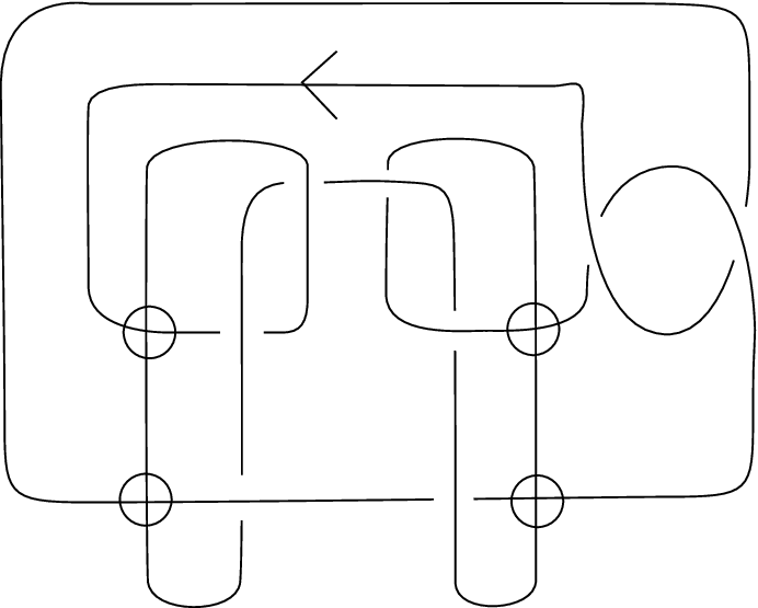
Remark.  M. B. Thistlethwaite [11] and K. Murasugi [10] showed that the $f$-polynomial (Jones polynomial) of a non-split alternating link is alternating, namely it is in a form of $A^{\alpha}\sum c_{i}A^{4i}$ such that $c_{i}c_{j}\geq 0$ for $i\equiv j\quad(\bmod\;2)$ and $c_{i}c_{j}\leq 0$ for $i\not\equiv j\quad(\bmod\;2)$. This does not hold in virtual knot theory. The $f$-polynomial of a virtual knot in Figure 10 is $A^{12}+3A^{16}-4A^{20}+3A^{24}-4A^{28}+4A^{32}-3A^{36}+A^{40}$.

References

- [1] M. Goussarov, M. Polyak, and O. Viro, Finite type invariants of classical and virtual knots, preprint (1998, math.GT/9810073).
- [2] V. F. R. Jones, A polynomial invariant for knots via von Neumann algebra, Bull. Amer. Math. Soc. 12 (1985), 103–111.
- [3] V. F. R. Jones, Hecke algebra representations of braid groups and link polynomials, Ann. of Math. 126 (1987), 335–388.
- [4] N. Kamada, Alternating link diagrams on compact oriented surfaces, preprint. (1995),
- [5] N. Kamada, The crossing number of alternating link diagrams of a surface, Proceedings of Knots 96, World Scientific Publishing Co., 1997, 377-382.
- [6] N. Kamada and S .Kamada, Abstract link diagrams and virtual knots, J. Knot Theory Ramifications 9 (2000), 93-106
- [7] L. H. Kauffman, State models and the Jones polynomial, Topology 26 (1987), 395–407
- [8] L. H. Kauffman, Talks at: the MSRI Meeting in January 1997: AMS Meeting at the University of Maryland College Park in March 1997; Knots in Hellas Meeting in Delphi, Greece in July 1998; APCTP-NANKAI Symposium on Yang-Baxter Systems, Non-Linear Models and Applications at Seoul, Korea in October 1998.
- [9] L. H. Kauffman, Virtual Knot Theory, Europ. J. Combinatorics 20 (1999) 663–690.
- [10] K. Murasugi, On invariants of graphs with applications to knot theory, Trans. Amer. Math. Soc. 314 (1989), 1–49.
- [11] M. B. Thistlethwaite, A spanning tree expansion of the Jones polynomial, Topology 26 (1987), 297–309.