跳到论文正文
W Papers独立论文阅读器 arXiv:math/0007166 论文正文 计算阅读时间 · 0%
引用这篇论文根据当前论文元数据生成,正式投稿前建议核对。


License: Assumed arXiv.org perpetual non-exclusive license
arXiv:math/0007166v1 [math.SG] 26 Jul 2000

Combinatorial formulas for products of Thom classesThanks: * Supported by NSF grant DMS 890771.Thanks: ** This research was partially conducted by the second author for the Clay Mathematics Institute.

Victor Guillemin11footnotemark: 1 * Address: Department of Mathematics, MIT, Cambridge, MA 02139 Email address: vwg@@math.mit.edu and Catalin Zara 22footnotemark: 2 ** Address: Department of Mathematics, MIT, Cambridge, MA 02139 Email address: czara@math.mit.edu
Abstract.

Let GG be a torus of dimension n>1n>1 and MM a compact Hamiltonian GG-manifold with MGM^{G} finite. A circle, S1S^{1}, in GG is generic if MG=MS1M^{G}=M^{S^{1}}. For such a circle the moment map associated with its action on MM is a perfect Morse function. Let {Wp+;p∈MG}\{W_{p}^{+};p\in M^{G}\} be the Morse-Whitney stratification of MM associated with this function, and let τp+\tau_{p}^{+} be the equivariant Thom class dual to Wp+W_{p}^{+}. These classes form a basis of HG∗​(M)H_{G}^{*}(M) as a module over 𝕊⁡(𝔤∗){\mathbb{S}}({\mathfrak{g}}^{*}) and, in particular,

τp+​τq+=∑cp​qr​τr+\tau_{p}^{+}\tau_{q}^{+}=\sum c_{pq}^{r}\tau_{r}^{+}

with cp​qr∈𝕊⁡(𝔤∗)c_{pq}^{r}\in{\mathbb{S}}({\mathfrak{g}}^{*}). For manifolds of GKM type we obtain a combinatorial description of these τp+\tau_{p}^{+}’s and, from this description, a combinatorial formula for cp​qrc_{pq}^{r}.

1. Products of Thom classes

Let M2​dM^{2d} be a compact Hamiltonian S1S^{1}-manifold with moment map, ϕ:M→ℝ\phi:M\to{\mathbb{R}}. If MS1M^{S^{1}} is finite, ϕ\phi is a Morse function, and its critical points, p∈MS1p\in M^{S^{1}}, are all of even index. This has important consequences for the topology of MM: If we put an S1S^{1}-invariant Riemannian metric, BB, on MM and let

v=∇Bϕv=\boldsymbol{\nabla}_{B}\phi

be the gradient vector field associated with BB and ϕ\phi, then, for every critical point, p∈MS1p\in M^{S^{1}}, the unstable manifold at pp:

Wp+={q∈M;limt→−∞(exptv)(q)=p}W^{+}_{p}=\{q\in M;\,\,\lim_{t\to-\infty}(\exp tv)(q)=p\}

supports a cohomology class, and these “Thom” classes

(1.1) τp+,p∈MS1\tau^{+}_{p},\quad p\in M^{S^{1}}

are an additive basis of the cohomology ring, H∗​(M,ℝ)H^{*}(M,{\mathbb{R}}). The same is true of the stable manifolds

Wp−={q∈M;limt→∞(exptv)(q)=p}W^{-}_{p}=\{q\in M;\,\,\lim_{t\to\infty}(\exp tv)(q)=p\}

and their dual Thom classes

τp−,p∈MS1.\tau^{-}_{p},\quad p\in M^{S^{1}}.

The main topic of this paper will be the symplectic version of what is sometimes called the multiplicative Morse problem: Given pp and qq in MS1M^{S^{1}}, τp+​τq+\tau^{+}_{p}\tau^{+}_{q} can be expanded as a sum

τp+​τq+=∑cp​qr​τr+.\tau^{+}_{p}\tau^{+}_{q}=\sum c^{r}_{pq}\tau^{+}_{r}\,.

What are the cp​qrc^{r}_{pq}’s? Closely related to this is the question of determining the cohomology pairings:

(1.2) cp​q​r=∫τp+​τq+​τr−.c_{pqr}=\int\tau^{+}_{p}\tau^{+}_{q}\tau^{-}_{r}\;.

Neither of these questions is easy to answer even when the structure of the cohomology ring itself is well understood. For instance if MM is the coadjoint orbit of a compact Lie group, the computation of the cp​qrc^{r}_{pq}’s is an important open problem in the theory of the Schubert calculus and is the focus of a lot of recent activity. (See, for instance, [BGG], [BH], [Bi], [Ko] and [Kn].)

In this paper we will consider the equivariant version of this problem. We will assume the action of S1S^{1} on MM can be extended to a Hamiltonian action of a torus, GG, of dimension n>1n>1, and replace the τp+\tau^{+}_{p}’s in (1.2) by their equivariant counterparts. These equivariant Thom classes generate HG​(M,ℝ)H_{G}(M,{\mathbb{R}}) as a module over the ring, HG​(p​t)=𝕊⁡(𝔤∗)H_{G}(pt)={\mathbb{S}}({\mathfrak{g}}^{*}), so one gets as above an identity

τp+​τq+=∑cp​qr​τr+,\tau^{+}_{p}\tau^{+}_{q}=\sum c^{r}_{pq}\tau^{+}_{r}\;,

but now the cp​qrc^{r}_{pq}’s are elements of the polynomial ring, 𝕊⁡(𝔤∗){\mathbb{S}}({\mathfrak{g}}^{*}). When

degree ​τr+=degree ​τp++degree ​τq+,\text{degree }\tau^{+}_{r}=\text{degree }\tau^{+}_{p}+\text{degree }\tau^{+}_{q}\;,

they are polynomials of degree zero (i.e. real numbers) and, in fact, coincide with the cp​qrc^{r}_{pq}’s in (1.2). Thus, they are in principle a much larger list of unknown quantities. We will show, however, that they are in some sense, easier to compute due to the fact that, in equivariant cohomology, one has a much richer store of intersection invariants to play around with. More explicitly if XX and YY are submanifolds of MM and τX\tau_{X} and τY\tau_{Y} their dual Thom classes, the intersection number

(1.3) #⁡(X∩Y)=∫τX​τY\#(X\cap Y)=\int\tau_{X}\tau_{Y}

is zero except when XX and YY are of complementary dimension. On the other hand if XX and YY are GG-invariant and τX\tau_{X} and τY\tau_{Y} their equivariant Thom classes, the expression (1.3) (which is now an element of 𝕊⁡(𝔤∗){\mathbb{S}}({\mathfrak{g}}^{*})) can be non-zero no matter what the relative dimensions of XX and YY are. Moreover, by the localization theorem of Atiyah-Bott-Berline-Vergne, (1.3), is a sum of local intersection invariants

#​(X∩Y)p∈Q⁡(𝔤∗),\#(X\cap Y)_{p}\in Q({\mathfrak{g}}^{*})\,,

where Q⁡(𝔤∗)Q({\mathfrak{g}}^{*}) is the quotient field of 𝕊⁡(𝔤∗){\mathbb{S}}({\mathfrak{g}}^{*}) and pp a fixed point, and each of these is itself an intersection invariant.

Of particular interest for us will be certain intersection invariants of this type associated with the moment map, ϕ\phi. Suppose that pp and qq are critical points of ϕ\phi and that there are no critical values of ϕ\phi in the interval (ϕ⁡(p),ϕ⁡(q))(\phi(p),\phi(q)). Let ϕ⁡(p)<c<ϕ⁡(q)\phi(p)<c<\phi(q) and let

Mc=ϕ−1​(c)/S1M_{c}=\phi^{-1}(c)/S^{1}

be the symplectic reduction of MM at cc. By the Marsden-Weinstein theorem, McM_{c} is a symplectic orbifold, and the action of GG on MM induces an action of the group

G1=G/S1G_{1}=G/S^{1}

on McM_{c}. The reduced spaces (Wp+)c(W^{+}_{p})_{c} and (Wq−)c(W^{-}_{q})_{c} are GG-invariant symplectic sub-orbifolds of McM_{c} and so their equivariant intersection “number”

(1.4) #⁡((Wp+)c∩(Wq−)c)\#((W^{+}_{p})_{c}\cap(W^{-}_{q})_{c})

is well-defined as an element of the subring, 𝕊⁡(𝔤1∗){\mathbb{S}}({\mathfrak{g}}^{*}_{1}), of 𝕊⁡(𝔤∗){\mathbb{S}}({\mathfrak{g}}^{*}). Moreover, if McG1M_{c}^{G_{1}} is finite, then for every v∈McG1v\in M^{G_{1}}_{c}, the local intersection number

(1.5) #​((Wp+)c∩(Wq−)c)v\#((W^{+}_{p})_{c}\cap(W^{-}_{q})_{c})_{v}

is well-defined as an element of Q⁡(𝔤1∗)Q({\mathfrak{g}}^{*}_{1}).

We will now describe the role of these intersection numbers in the computation of the cp​qrc^{r}_{pq}’s. We will say that MM is a GKM manifold if, for all non-critical values, cc, McG1M_{c}^{G_{1}} is finite. Thus, being GKM is a necessary and sufficient condition for the invariants (1.5) to be well-defined. We recall some other characterizations of these manifolds.

Theorem 1.1.

MM is GKM if and only if, for every p∈MGp\in M^{G}, the weights, αi,p\alpha_{i,p}, of the linear isotropy representation of GG on Tp​MT_{p}M are pair-wise linearly independent; i.e, αi,p\alpha_{i,p} is not a multiple of αj,p\alpha_{j,p} if i≠ji\neq j.

Theorem 1.2.

MM is GKM if and only if, for every codimension one subtorus, HH, of GG the connected components of MHM^{H} are either fixed points of GG or imbedded copies of S2S^{2}. Moreover, if a connected component, XX, is a copy of S2S^{2}, the action of GG on XX is symplectomorphic to the standard action of G/H=S1G/H=S^{1} on S2S^{2}.

Theorem 1.3.

MM is GKM if and only if the one skeleton of MM

(1.6) {p∈M,dimGp≥n−1}\{p\in M,\quad\dim G_{p}\geq n-1\}

is a finite union of embedded S2S^{2}’s.

Proof.

Theorem 1.3 is an obvious consequence of Theorem 1.2; and it is easy to see that if the hypotheses of Theorem 1.2 hold, MM is GKM. For the other implications see [GZ2]. ∎

The intersection properties of the embedded S2S^{2}’s in the set (1.6) can be described by an intersection graph, and a beautiful observation of Goresky-Kottwitz-MacPherson is that one can read off the structure of the equivariant cohomology ring of MM from the “action” of GG on this graph. More explicitly let Γ\Gamma be the graph whose vertices are the fixed points of GG and whose edges, ee, are copies, XeX_{e}, of the S2S^{2}’s in Theorem 1.3. The graph structure on this collection of vertices and edges is given by defining the pair of vertices incident to an edge, ee, to be the set

∂e={p,q}=XeG.\partial e=\{p,q\}=X^{G}_{e}\,.

In particular, if ee is an oriented edge, its initial vertex, i⁡(e)i(e), is defined to be the “south pole”, pp, of the two-sphere, XeX_{e}, and its terminal vertex, t⁡(e)t(e), to be the “north pole”, qq of XeX_{e}. The action of GG on the set (1.6) can be described graph theoretically by two pieces of data: a function ρ\rho which assigns to each oriented edge, ee, of Γ\Gamma a one-dimensional representation, ρe\rho_{e}, of GG and a function, κ\kappa, which assigns to each vertex, pp, a dd-dimensional representation, κp\kappa_{p}. These functions are defined by letting ρe\rho_{e} be the representation of GG on Tp​XeT_{p}X_{e}, p=i⁡(e)p=i(e), and letting κp\kappa_{p} be the representation of GG on Tp​MT_{p}M. It is easily checked that ρ\rho and κ\kappa satisfy the axioms:

(1.7) κp\displaystyle\kappa_{p} =⨁i⁡(e)=pρe\displaystyle=\bigoplus_{i(e)=p}\rho_{e}
(1.8) ρe¯\displaystyle\rho_{\bar{e}} =ρe∗\displaystyle=\rho^{*}_{e}
and
(1.9) κp|Ge\displaystyle\kappa_{p}|_{G_{e}} =κq|Ge\displaystyle=\kappa_{q}|_{G_{e}}

where e¯\bar{e} is the edge obtained from ee by reversing its orientation, GeG_{e} is the kernel of ρe\rho_{e} and pp and qq are the vertices i⁡(e)i(e) and t⁡(e)t(e). In particular, by (1.7), κp\kappa_{p} is determined by the ρe\rho_{e}’s with i⁡(e)=pi(e)=p. Since ρe\rho_{e} is a one-dimensional representation it is determined by its weight, αe\alpha_{e}; so the “action” of GG on Γ\Gamma associated with ρ\rho and κ\kappa consists essentially of a labeling of the oriented edges, ee, of Γ\Gamma by weights, αe\alpha_{e}. The axioms (1.7)–(1.9) impose, of course, some condition on this labeling. For instance (1.8) is equivalent to

αe=−αe¯.\alpha_{e}=-\alpha_{\bar{e}}\,.

Now let HG​(M)H_{G}(M) be the equivariant cohomology ring of MM and HG​(MG)H_{G}(M^{G}) the equivariant cohomology ring of MGM^{G}. Since MGM^{G} is a finite disjoint union of fixed points and these fixed points are also the vertices, VΓV_{\Gamma}, of Γ\Gamma it follows that

HG​(MG)=Maps⁡(VΓ,𝕊⁡(𝔤∗)).H_{G}(M^{G})=\operatorname{Maps}(V_{\Gamma},{\mathbb{S}}({\mathfrak{g}}^{*}))\,.

Moreover, if i:MG→Mi:M^{G}\to M is the inclusion, the map i∗:HG​(M)→HG​(MG)i^{*}:H_{G}(M)\to H_{G}(M^{G}) is injective, by a well-known result of Kirwan. The theorem of Goresky-Kottwitz-MacPherson which we alluded to above asserts:

Theorem 1.4.

A map h:VΓ→S⁡(𝔤∗)h:V_{\Gamma}\to S({\mathfrak{g}}^{*}) is in the image of i∗i^{*} if and only if, for every edge, ee, of Γ\Gamma

(1.10) hp|𝔤e=hq|𝔤eh_{p}|_{{\mathfrak{g}}_{e}}=h_{q}|_{{\mathfrak{g}}_{e}}

pp and qq being the vertices of ee and 𝔤e{\mathfrak{g}}_{e} the annihilator of αe\alpha_{e} in 𝔤{\mathfrak{g}}.

This leads us to define the equivariant cohomology ring, H⁡(Γ,α)H(\Gamma,\alpha) of Γ\Gamma to be the set of all maps, h:VΓ→S⁡(𝔤∗)h:V_{\Gamma}\to S({\mathfrak{g}}^{*}) satisfying (1.10). Each of the Thom classes (1.1) gets mapped by i∗i^{*} onto an element of H⁡(Γ,α)H(\Gamma,\alpha) and we will continue to use the notation, τp+\tau^{+}_{p}, for this “combinatorial” Thom class. The main result of this article is a formula for this Thom class as a kind of path integral over certain paths in Γ\Gamma. Before stating this result we’ll describe a few basic properties of these combinatorial Thom classes. Lets continue to denote by ϕ\phi the restriction of the moment map, ϕ\phi, to MGM^{G}. Identifying MGM^{G} with VΓV_{\Gamma}, one can think of ϕ\phi as a real-valued function on VΓV_{\Gamma}. By Theorem 1.2, ϕ\phi takes on distinct values on the vertices i⁡(e)i(e) and t⁡(e)t(e) of an oriented edge, ee. We will say that this edge is ascending if ϕ⁡(i⁡(e))<ϕ⁡(t⁡(e))\phi(i(e))<\phi(t(e)) and descending if the reverse inequality is true. More generally if γ\gamma is a path in Γ\Gamma we will say that γ\gamma is ascending if each of its edges is ascending. For every vertex, p∈VΓp\in V_{\Gamma} define the index, σp\sigma_{p}, of pp to be the number of descending edges, ee, with i⁡(e)=pi(e)=p.

Theorem 1.5.

The Thom class, τp+\tau^{+}_{p}, has the following properties:

  1. (1)

    Its support is the set of all vertices of Γ\Gamma which can be joined to pp by an ascending path.

  2. (2)

    The value of τp+\tau^{+}_{p} at pp is

    νp+=∏′i⁡(e)=p′​αe,\nu_{p}^{+}=\sideset{}{{}^{\prime}}{\prod}_{i(e)=p}\alpha_{e}\quad,

    the product, ∏′\prod^{\prime}, being over all descending edges with i⁡(e)=pi(e)=p.

In certain instances these properties uniquely characterize τp+\tau^{+}_{p}.

Theorem 1.6.

Suppose that the indexing function, σ:VΓ→ℤ\sigma:V_{\Gamma}\to{\mathbb{Z}}, p→σpp\to\sigma_{p}, is strictly increasing along ascending paths. Then τp+\tau^{+}_{p} is the unique element of H⁡(Γ,α)H(\Gamma,\alpha) with properties 1 and 2 above.

We will now describe our “path-integral” formula for τp+\tau^{+}_{p}. As mentioned above this formula will involve the Hamiltonian action of the subgroup, S1S^{1}, of GG on MM and the intersection invariants (1.4) and (1.5). Let ξ∈𝔤\xi\in{\mathfrak{g}} be the infinitesimal generator of this subgroup and let ee be an ascending edge of Γ\Gamma with p=i⁡(e)p=i(e). For any point, cc, on the interval between ϕ⁡(p)\phi(p) and ϕ⁡(q)\phi(q), the S1S^{1}-reduced space, (Xe)c(X_{e})_{c} consists of a single point, v∈Mcv\in M_{c}. Let ιe\iota_{e} be the local intersection number (1.5).

Theorem 1.7.

For every q∈VΓq\in V_{\Gamma}

(1.11) τp+​(q)=∑E⁡(γ)\tau^{+}_{p}(q)=\sum E(\gamma)

the sum being over all ascending paths, γ\gamma, joining pp to qq, and the summands being defined by

(1.12) E⁡(γ)=(−1)m​νq+​ιe1α^m​∏k=2mιekα^k−1−α^k,E(\gamma)=(-1)^{m}\nu_{q}^{+}\frac{\iota_{e_{1}}}{\hat{\alpha}_{m}}\prod^{m}_{k=2}\frac{\iota_{e_{k}}}{\hat{\alpha}_{k-1}-\hat{\alpha}_{k}}\;,

where e1,…,eme_{1},\ldots,e_{m} are the edges of γ\gamma and

α^k=αekαek​(ξ).\hat{\alpha}_{k}=\frac{\alpha_{e_{k}}}{\alpha_{e_{k}}(\xi)}\,.

Remarks:

  1. (1)

    The local intersection number, ιe\iota_{e}, is equal to the global intersection number (1.4) provided that there are no ascending paths in Γ\Gamma of length greater than one joining p=i⁡(e)p=i(e) to q=t⁡(e)q=t(e). In particular, if γ\gamma is a longest path joining pp to qq all the intersection numbers in (1.12) are global intersection numbers and in particular are elements of 𝕊⁡(𝔤∗){\mathbb{S}}({\mathfrak{g}}^{*}).

  2. (2)

    In Section 4 we will give a purely combinatorial definition of ιe\iota_{e}.

As a corollary of Theorem 1.5 one gets for (1.2) the formula

(1.13) cp​q​r=∑tδt​E​(γ1)​E​(γ2)​E​(γ3)c_{pqr}=\sum_{t}\delta_{t}E(\gamma_{1})E(\gamma_{2})E(\gamma_{3})

summed over all configurations of paths, γ1\gamma_{1}, γ2\gamma_{2} and γ3\gamma_{3}, where γ1\gamma_{1} is an ascending path from pp to tt, γ2\gamma_{2} an ascending path from qq to tt, γ3\gamma_{3} a descending path from rr to tt and

δt=(∏i⁡(e)=tαe)−1.\delta_{t}=\Bigl(\prod_{i(e)=t}\alpha_{e}\Bigr)^{-1}\,.

In particular:

Theorem 1.8.

If the hypotheses of Theorem 1.6 are satisfied, cp​qr=cp​q​rc^{r}_{pq}=c_{pqr} and hence cp​qrc^{r}_{pq} is equal to the sum (1.13).

A few words about the organization of this paper. In Section 2 we will give a brief account of the theory of GG-actions on graphs (based, for the most part, on material in [GZ3]). In Section 3 we will derive a preliminary version of Theorem 1.7 and then, in Section  4, deduce from it the version above, after first describing how to define the invariants (1.5) combinatorially. In Section 5 we will attempt to demystify what is perhaps the most puzzling feature of the formula (1.11), the fact that all the summands are rational functions (elements of the quotient field, Q⁡(𝔤∗)Q({\mathfrak{g}}^{*})), whereas the sum itself is a polynomial. This indicates that a lot of mysterious cancellations are occurring in this summation; and we will show how these cancellations occur in a few simple but enlightening examples.

We would like to thank Tara Holm and Sue Tolman for helping us with the computations involved in these examples and Allen Knutson for pointing out to us antecedents in the combinatorial literature for formulas of type (1.11) and (1.13).

2. GG-actions on graphs

Let Γ\Gamma be a finite dd-valent graph. Given an oriented edge, ee, of Γ\Gamma we will denote by i⁡(e)i(e) the initial vertex of ee and by t⁡(e)t(e) the terminal vertex; and we will denote by e¯\bar{e} the edge obtained from ee by reversing its orientation. Thus i⁡(e¯)=t⁡(e)i(\bar{e})=t(e) and t⁡(e¯)=i⁡(e)t(\bar{e})=i(e).

Definition 2.1.

Let ρ\rho be a function which assigns to each oriented edge, ee, of Γ\Gamma a one dimensional representation, ρe:G→S1\rho_{e}:G\to S^{1}; and let κ\kappa be a function which assigns to each vertex, pp, a dd-dimensional representation of G,κpG,\kappa_{p}. We will say that ρ\rho and κ\kappa define an action of GG on Γ\Gamma if the axioms (1.7)–(1.9) are satisfied.

Let αe\alpha_{e} be the weight of the representation ρe\rho_{e}. By (1.7), the weights, αe,i⁡(e)=p\alpha_{e},i(e)=p, determine the representation κp\kappa_{p} up to isomorphism; so the action of GG on Γ\Gamma is basically just a labeling of the edges of Γ\Gamma by weights. We will denote the function, e→αee\to\alpha_{e}, by α\alpha and call it the axial function of the action of GG on Γ\Gamma. The axioms (1.7)–(1.9) can be reformulated as statements about α\alpha:

Proposition 2.2.

Axiom (1.8) is satisfied iff

αe=−αe¯\alpha_{e}=-\alpha_{\bar{e}}

and axiom (1.9) is satisfied iff one can order the weights

αek,\displaystyle\alpha_{e_{k}}\;, i⁡(ek)=p,ek≠e\displaystyle\quad i(e_{k})=p,\,e_{k}\neq e
and the weights
αek′,,\displaystyle\alpha_{e^{\prime}_{k}},\;, i⁡(ek′)=q,ek′≠e¯\displaystyle\quad i(e^{\prime}_{k})=q,\,e^{\prime}_{k}\neq\bar{e}

so that

(2.1) αek′=αek+ck​αe.\alpha_{e^{\prime}_{k}}=\alpha_{e_{k}}+c_{k}\alpha_{e}\,.

(We will leave the proof of these assertions as an easy exercise.)

Definition 2.3.

The action of GG on Γ\Gamma is a GKM action if, for all vertices, pp, the weights, αe,i⁡(e)=p\alpha_{e},i(e)=p, are pair-wise linear independent.

From now on we will assume, unless we state otherwise, that the action of GG on Γ\Gamma has this property.

For every vertex, pp, of Γ\Gamma let EpE_{p} be the set of oriented edges, ee, with i⁡(e)=pi(e)=p.

Definition 2.4.

A connection on Γ\Gamma is a function which assigns to every oriented edge, ee, a bijective map

θe:Ei⁡(e)→Et⁡(e)\theta_{e}:E_{i(e)}\to E_{t(e)}

satisfying θe¯=θe−1\theta_{\bar{e}}=\theta^{-1}_{e}. This connection is compatible with the action of GG if, for every oriented edge, ee, with i⁡(e)=pi(e)=p and every edge, ek∈Ep,ek≠ee_{k}\in E_{p},\,e_{k}\neq e

(2.2) αek′=αek+ck​αe, where ​ek′=θe​(ek).\alpha_{e^{\prime}_{k}}=\alpha_{e_{k}}+c_{k}\alpha_{e},\quad\text{ where }e^{\prime}_{k}=\theta_{e}(e_{k})\,.

Thus the existence of a GG-compatible connection is a slight sharpening of the identity (2.1). It is easy to see that GG-compatible connections exist, and we will assume henceforth that Γ\Gamma is equipped with such a connection.

Let VΓV_{\Gamma} be the set of vertices of Γ\Gamma and EΓE_{\Gamma} the set of oriented edges. Motivated by the theorem of Goresky–Kottwitz–MacPherson we define the equivariant cohomology ring, H⁡(Γ,α)H(\Gamma,\alpha), of Γ\Gamma to be the set of maps, h:VΓ→𝕊⁡(𝔤∗)h:V_{\Gamma}\to{\mathbb{S}}({\mathfrak{g}}^{*}), satisfying the compatibility condition (1.10) for all e∈EΓe\in E_{\Gamma}. This ring has a natural grading33 3 This definition is, unfortunately, inconsistent with the topological definition which assigns to HkH^{k} the degree 2​k2k. (It is, however, more natural in this algebraic context.)

Hk​(Γ,α)=H⁡(Γ,α)∩Maps⁡(VΓ,𝕊k​(𝔤∗))H^{k}(\Gamma,\alpha)=H(\Gamma,\alpha)\cap\operatorname{Maps}(V_{\Gamma},{\mathbb{S}}^{k}({\mathfrak{g}}^{*}))

and contains 𝕊⁡(𝔤∗){\mathbb{S}}({\mathfrak{g}}^{*}) as a subring: the ring of constant maps of VΓV_{\Gamma} into 𝕊⁡(𝔤∗){\mathbb{S}}({\mathfrak{g}}^{*}). The proof of Theorem 1.7 will require a number of results about the structure of H⁡(Γ,α)H(\Gamma,\alpha) as an 𝕊⁡(𝔤∗){\mathbb{S}}({\mathfrak{g}}^{*}) module. These results were proved in an earlier paper of ours on “equivariant Morse theory on graphs” ([GZ3]), and we will refer to this paper for a detailed treatment of the material in the next few paragraphs. Let

(2.3) 𝒫={ξ∈𝔤,αe(ξ)≠0 for all e∈EΓ}.{\mathcal{P}}=\{\xi\in{\mathfrak{g}},\alpha_{e}(\xi)\neq 0\hbox{ for all }e\in E_{\Gamma}\}\,.

Given an element, ξ∈𝒫\xi\in{\mathcal{P}}, we will say that an oriented edge, ee, is ascending with respect to ξ\xi if αe​(ξ)>0\alpha_{e}(\xi)>0. For every vertex, pp, let σp\sigma_{p}, the index of pp, be the number of ascending edges, ee, with t⁡(e)=pt(e)=p.

Definition 2.5.

The kt​hk^{th} Betti number, bk​(Γ)b_{k}(\Gamma), is the number of vertices, pp, of Γ\Gamma for which σp=k\sigma_{p}=k.

Remark: The definition of σp\sigma_{p} depends upon the choice of ξ\xi but bk​(Γ)b_{k}(\Gamma) turns out not to. (See [GZ1, Theorem 2.6]).

A function ϕ:VΓ→ℝ\phi:V_{\Gamma}\to{\mathbb{R}} is a (ξ\xi-compatible) Morse function if, for every ascending edge ee, ϕ⁡(i⁡(e))<ϕ⁡(t⁡(e))\phi(i(e))<\phi(t(e)). It is not obvious, and in fact not true, that Morse functions exist. A necessary and sufficient condition for the existence of a Morse function is that, for every ascending path in Γ\Gamma the initial vertex of this path is distinct from its terminal vertex (i.e., there are no ascending “loops”). If a Morse function exists, however, one can easily perturb it so that it is injective as a map of VΓV_{\Gamma} into ℝ{\mathbb{R}}. From now on we will let ϕ\phi be a fixed Morse function with this property.

The topological results discussed in Section 1 prompt one to make the following Morse-theoretic conjectures about the equivariant cohomology ring of a graph.

Conjecture 1.

H⁡(Γ,α)H(\Gamma,\alpha) is a free 𝕊⁡(𝔤∗){\mathbb{S}}({\mathfrak{g}}^{*}) module with bk​(Γ)b_{k}(\Gamma) generators of degree kk.

Conjecture 2.

H⁡(Γ,α)H(\Gamma,\alpha) is freely generated as an S⁡(𝔤∗)S({\mathfrak{g}}^{*}) module by a family of “Thom classes”

τp+∈Hk​(Γ,α),k=σp,\tau^{+}_{p}\in H^{k}(\Gamma,\alpha),\,\,k=\sigma_{p}\,,

satisfying

(2.4) support ​τp+⊆Fp\hbox{support }\tau^{+}_{p}\subseteq F_{p}

and

(2.5) τp+​(p)=∏e∈Ep−αe(:=νp+),\tau^{+}_{p}(p)=\prod_{e\in E^{-}_{p}}\alpha_{e}\,\quad(:=\nu_{p}^{+})\;,

FpF_{p} being the set of vertices which can be joined to pp by an ascending path and Ep−E^{-}_{p} being the set of descending edges in EpE_{p}.

It is clear that Conjecture 2 implies Conjecture 1, and it is not difficult to prove that Conjecture 1 implies Conjecture 2 (see [GZ2, §2.4.3]). Therefore, since Conjecture 1 doesn’t depend on the choice of an orientation of Γ\Gamma (i.e. the choice of a polarizing vector ξ∈𝒫\xi\in{\mathcal{P}}), the same is true of Conjecture 2. In particular, if we reverse the orientation (replace ξ\xi by −ξ-\xi), we get from Conjecture 2 the existence of Thom classes, τp−\tau_{p}^{-}, p∈VΓp\in V_{\Gamma}, associated with the Morse function −ϕ-\phi.

Unfortunately these conjectures are not true in general; however there is a useful necessary and sufficient condition for them to be true involving certain subgraphs of Γ\Gamma.

Definition 2.6.

A subgraph, Γ1\Gamma_{1}, of Γ\Gamma is totally geodesic if, for every pair of edges, ee and e′e^{\prime}, of Γ1\Gamma_{1}, with i⁡(e)=i⁡(e′)i(e)=i(e^{\prime}), θe​(e′)\theta_{e}(e^{\prime}) is also an edge of Γ1\Gamma_{1}.

Note that if Γ1\Gamma_{1} is a totally geodesic subgraph of Γ\Gamma the restriction to it of α\alpha is, by (2.2), an axial function on Γ1\Gamma_{1}; so each of these subgraphs is equipped with an action of GG. An important example of a totally geodesic subgraph is the following. Let 𝔥∗{\mathfrak{h}}^{*} be a subspace of 𝔤∗{\mathfrak{g}}^{*}, and let Γ𝔥∗\Gamma_{{\mathfrak{h}}^{*}} be the subgraph whose edges are the set

{e∈EΓ,αe∈𝔥∗}.\{e\in E_{\Gamma},\alpha_{e}\in{\mathfrak{h}}^{*}\}\,.

(It is clear, by (2.1) and (2.2) that this is totally geodesic.) One of the main results of [GZ3] is the following.

Theorem 2.7.

Conjecture 2 is true for Γ\Gamma if and only if, for every two-dimensional subspace, 𝔥∗{\mathfrak{h}}^{*}, of 𝔤∗{\mathfrak{g}}^{*}, Conjecture 2 is true for Γ𝔥∗\Gamma_{{\mathfrak{h}}^{*}}.

Thus, to verify that Conjecture 2 holds for Γ\Gamma it suffices to verify it for these subgraphs (which is usually much easier than verifying it for Γ\Gamma itself).

The proof of Theorem 2.7 involves a graph-theoretic version of symplectic reduction. We will say that cc is a critical value of the Morse function ϕ:VΓ→ℝ\phi:V_{\Gamma}\to{\mathbb{R}} if c=ϕ⁡(p)c=\phi(p) for some p∈VΓp\in V_{\Gamma} and, otherwise, cc is a regular value. Let cc be a regular value of ϕ\phi and let VcV_{c} be the set of oriented edges, ee, of Γ\Gamma with ϕ⁡(i⁡(e))<c<ϕ⁡(t⁡(e))\phi(i(e))<c<\phi(t(e)). We show in [GZ3] that VcV_{c} is the set of vertices of a hypergraph, Γc\Gamma_{c}. Thus the elements of VcV_{c} are both edges of the graph Γ\Gamma and vertices of this hypergraph. It is useful to distinguish between the two roles they play by saying that “an edge, ee, intersects Γc\Gamma_{c} in a vertex, vev_{e}.”

Let 𝔤ξ∗{\mathfrak{g}}^{*}_{\xi} be the annihilator of ξ\xi in 𝔤∗{\mathfrak{g}}^{*}. For each oriented edge, ee, of Γ\Gamma we define a map ρe:𝔤∗→𝔤ξ∗\rho_{e}:{\mathfrak{g}}^{*}\to{\mathfrak{g}}^{*}_{\xi} by setting

ρe​α=α−α⁡(ξ)αe​(ξ)​αe.\rho_{e}\alpha=\alpha-\frac{\alpha(\xi)}{\alpha_{e}(\xi)}\alpha_{e}\,.

This extends to a ring homomorphism

(2.6) ρe:𝕊⁡(𝔤∗)→𝕊⁡(𝔤ξ∗)\rho_{e}:{\mathbb{S}}({\mathfrak{g}}^{*})\to{\mathbb{S}}({\mathfrak{g}}^{*}_{\xi})

and, from (2.6), we get a ring homomorphism

𝒦c:H⁡(Γ,α)→Maps⁡(Vc,𝕊⁡(𝔤ξ∗)){\mathcal{K}}_{c}:H(\Gamma,\alpha)\to\operatorname{Maps}(V_{c},{\mathbb{S}}({\mathfrak{g}}^{*}_{\xi}))

by setting

(2.7) 𝒦c​(g)​(ve)=ρe​gi⁡(e)=ρe​gt⁡(e).{\mathcal{K}}_{c}(g)(v_{e})=\rho_{e}g_{i(e)}=\rho_{e}g_{t(e)}\,.

(The two terms on the right are equal by (1.10).)

We show in [GZ3] that 𝒦c{\mathcal{K}}_{c} maps H⁡(Γ,α)H(\Gamma,\alpha) into the cohomology ring, H⁡(Γc,αc)H(\Gamma_{c},\alpha_{c}), of the hypergraph Γc\Gamma_{c}. We won’t bother to review here the definition of this hypergraph cohomology ring (which is quite tricky) since one of the main theorems of [GZ3] asserts that, if the hypotheses of Theorem 2.7 hold and if ξ\xi satisfies a certain genericity condition (which we will spell out below), the map

𝒦c:H⁡(Γ,α)→H⁡(Γc,αc){\mathcal{K}}_{c}:H(\Gamma,\alpha)\to H(\Gamma_{c},\alpha_{c})

is a submersion. Hence, thanks to this theorem, one can define H⁡(Γc,αc)H(\Gamma_{c},\alpha_{c}) to be the image of 𝒦c{\mathcal{K}}_{c}.

A key step in the proof of Theorem 2.7 is a theorem which describes how the structure of the ring H⁡(Γc,αc)H(\Gamma_{c},\alpha_{c}) changes as one passes through a critical value of cc. More explicitly suppose cc and c′c^{\prime} are regular values of ϕ\phi and suppose that there exists a unique vertex, pp, with c<ϕ⁡(p)<c′c<\phi(p)<c^{\prime}. In addition suppose that, for e1e_{1}, e2e_{2}, e3e_{3}, e4∈Epe_{4}\in E_{p}

(2.8) 1αe1​(ξ)​ρe2​αe1≠1αe3​(ξ)​ρe4​αe3\frac{1}{\alpha_{e_{1}}(\xi)}\rho_{e_{2}}\alpha_{e_{1}}\neq\frac{1}{\alpha_{e_{3}}(\xi)}\rho_{e_{4}}\alpha_{e_{3}}

except when the two sides of (2.8) are forced to be equal (i.e., except when e1=e2e_{1}=e_{2} and e3=e4e_{3}=e_{4} or e1=e3e_{1}=e_{3} and e2=e4e_{2}=e_{4}). The inequality (2.8) is unfortunately not satisfied for all elements, ξ\xi, of the set (2.3), but one can show that those ξ\xi’s for which it is satisfied form an open dense subset of this set.

Let rr be the index of pp and let s=d−rs=d-r. Let ei,i=1,…,re_{i},i=1,\ldots,r be the descending edges in EpE_{p} and ea,a=r+1,…,de_{a},a=r+1,\ldots,d be the ascending edges in EpE_{p}. Let

Δc\displaystyle\Delta_{c} ={ei;i=1,…,r}\displaystyle=\{e_{i};i=1,\ldots,r\}
and
Δc′\displaystyle\Delta_{c^{\prime}} ={ea;a=r+1,…,d}.\displaystyle=\{e_{a};a=r+1,\ldots,d\}\,.

Then Δc\Delta_{c} is a subset of VcV_{c}, Δc′\Delta^{\prime}_{c} a subset of VcV_{c} and

Vc−Δc=Vc′−Δc′=V0,V_{c}-\Delta_{c}=V_{c^{\prime}}-\Delta_{c^{\prime}}=V_{0}\;,

where V0V_{0} is the intersection of VcV_{c} and Vc′V_{c^{\prime}}. Let

V#=V0∪(Δc×Δc′).V^{\#}=V_{0}\cup(\Delta_{c}\times\Delta_{c^{\prime}})\,.

Then one has projection maps

πc:V#→Vcandπc′:V#→Vc′\pi_{c}:V^{\#}\to V_{c}\quad\text{and}\quad\pi_{c^{\prime}}:V^{\#}\to V_{c^{\prime}}

and, from these projection maps, pull-back maps, πc∗\pi^{*}_{c} and πc′∗\pi^{*}_{c^{\prime}}, embedding the rings

(2.9) Maps⁡(Vc,𝕊⁡(𝔤ξ∗))\operatorname{Maps}(V_{c},{\mathbb{S}}({\mathfrak{g}}^{*}_{\xi}))

and

(2.10) Maps⁡(Vc′,𝕊⁡(𝔤ξ∗))\operatorname{Maps}(V_{c^{\prime}},{\mathbb{S}}({\mathfrak{g}}^{*}_{\xi}))

into the ring

(2.11) Maps⁡(V#,𝕊⁡(𝔤ξ∗)).\operatorname{Maps}(V^{\#},{\mathbb{S}}({\mathfrak{g}}^{*}_{\xi}))\,.

Moreover the ring

(2.12) Maps⁡(Δc,𝕊⁡(𝔤ξ∗))\operatorname{Maps}(\Delta_{c},{\mathbb{S}}({\mathfrak{g}}^{*}_{\xi}))

sits in the ring (2.9) as the set of maps h:Vc→𝕊⁡(𝔤ξ∗)h:V_{c}\to{\mathbb{S}}({\mathfrak{g}}^{*}_{\xi}) supported on Δc\Delta_{c}, and the ring

(2.13) Maps⁡(Δc′,𝕊⁡(𝔤ξ∗))\operatorname{Maps}(\Delta^{\prime}_{c},{\mathbb{S}}({\mathfrak{g}}^{*}_{\xi}))

sits inside the ring (2.10); so all the rings (2.9)–(2.13) can be regarded as subrings of (2.11).

Let y1,…,yn−1y_{1},\ldots,y_{n-1} be a basis of 𝔤ξ∗{\mathfrak{g}}^{*}_{\xi} and xx a fixed element of 𝔤∗{\mathfrak{g}}^{*} with ⟨x,ξ⟩=1\langle x,\xi\rangle=1. Let

αei\displaystyle\alpha_{e_{i}} =mi(x−βa(y))i=1,…,r\displaystyle=m_{i}(x-\beta_{a}(y))\qquad i=1,\ldots,r
and
αea\displaystyle\alpha_{e_{a}} =ma(x−βa(y))a=r+1,…,d,\displaystyle=m_{a}(x-\beta_{a}(y))\qquad a=r+1,\ldots,d\;,

with mi<0<mam_{i}<0<m_{a} and with the β\beta’s in 𝔤ξ∗{\mathfrak{g}}^{*}_{\xi}. Consider the maps

τc\displaystyle\tau_{c} :Δc→𝔤ξ∗,\displaystyle:\Delta_{c}\to{\mathfrak{g}}^{*}_{\xi}\,, τc​(ei)\displaystyle\,\tau_{c}(e_{i}) =βi\displaystyle=\beta_{i}
τc′\displaystyle\tau_{c^{\prime}} :Δc′→𝔤ξ∗,\displaystyle:\Delta_{c^{\prime}}\to{\mathfrak{g}}^{*}_{\xi}\,, τc′​(ea)\displaystyle\,\tau_{c^{\prime}}(e_{a}) =βa\displaystyle=\beta_{a}
and
τ#\displaystyle\tau^{\#} :Δc×Δc′→𝔤ξ∗,\displaystyle:\Delta_{c}\times\Delta_{c^{\prime}}\to{\mathfrak{g}}^{*}_{\xi}\,, τ#​(ei,ea)\displaystyle\,\tau^{\#}(e_{i},e_{a}) =βi−βa.\displaystyle=\beta_{i}-\beta_{a}\,.

The first two of these maps depend on the choice of xx; however, τ#\tau^{\#} is intrinsically defined since τ#​(ei,ea)\tau^{\#}(e_{i},e_{a}) is just

1αei​(ξ)​ρea​αei.\frac{1}{\alpha_{e_{i}}(\xi)}\rho_{e_{a}}\alpha_{e_{i}}\,.

Also, by the genericity condition (2.8) the map, τ#\tau^{\#} sends Δc×Δc′\Delta_{c}\times\Delta^{\prime}_{c} injectively into 𝔤ξ∗{\mathfrak{g}}^{*}_{\xi} and, as a consequence, τc\tau_{c} and τc′\tau^{\prime}_{c} map Δc\Delta_{c} and Δc′\Delta_{c^{\prime}} injectively into 𝔤ξ∗{\mathfrak{g}}^{*}_{\xi}.

Define the cohomology ring, H⁡(Δc,τc)H(\Delta_{c},\tau_{c}), to be the set of all maps of Δc\Delta_{c} into 𝕊⁡(𝔤ξ∗){\mathbb{S}}({\mathfrak{g}}^{*}_{\xi}) of the form

h=∑i=0r−1gi​τci,gi∈𝕊⁡(𝔤ξ∗)h=\sum^{r-1}_{i=0}g_{i}\tau^{i}_{c}\quad,\quad g_{i}\in{\mathbb{S}}({\mathfrak{g}}^{*}_{\xi})

and define H⁡(Δc′,τc′)H(\Delta_{c^{\prime}},\tau_{c^{\prime}}) to be the set of all maps of Δc′\Delta_{c^{\prime}} into 𝕊⁡(𝔤ξ∗){\mathbb{S}}({\mathfrak{g}}^{*}_{\xi}) of the form

h′=∑i=0s−1gi′​τc′i,gi′∈𝕊⁡(𝔤ξ∗).h^{\prime}=\sum^{s-1}_{i=0}g^{\prime}_{i}\tau^{i}_{c^{\prime}}\quad,\quad g^{\prime}_{i}\in{\mathbb{S}}({\mathfrak{g}}^{*}_{\xi})\,.

The theorem we alluded to above asserts

Theorem 2.8.

For every f∈H⁡(Γc,αc)f\in H(\Gamma_{c},\alpha_{c}) and every fi∈H⁡(Δc,τc)f_{i}\in H(\Delta_{c},\tau_{c}), i=1,…,s−1i=1,\ldots,s-1, there exists a unique f′∈H⁡(Γc′,αc′)f^{\prime}\in H(\Gamma_{c^{\prime}},\alpha_{c^{\prime}}) and unique fj′∈H⁡(Δc′,τc′)f^{\prime}_{j}\in H(\Delta_{c^{\prime}},\tau_{c^{\prime}}), j=1,…,r−1j=1,\ldots,r-1 such that

(2.14) f′+∑j=1r−1(τ#)j​fj′=f+∑i=1s−1(τ#)i​fi.f^{\prime}+\sum^{r-1}_{j=1}(\tau^{\#})^{j}f^{\prime}_{j}=f+\sum^{s-1}_{i=1}(\tau^{\#})^{i}f_{i}\,.

Remarks:

  1. (1)

    This theorem gives one a concrete picture of how H⁡(Γc,αc)H(\Gamma_{c},\alpha_{c}) changes as one goes through a critical point of ϕ\phi. Namely it shows that H⁡(Γc′,αc′)H(\Gamma_{c^{\prime}},\alpha_{c^{\prime}}) can be obtained from H⁡(Γc,αc)H(\Gamma_{c},\alpha_{c}) by a “blow-up” followed by a “blow-down”. (Compare with [GZ2, Theorem 2.3.2].)

  2. (2)

    This theorem can also be used to map cohomology classes in H⁡(Γc,αc)H(\Gamma_{c},\alpha_{c}) into cohomology classes in H⁡(Γc′,αc′)H(\Gamma_{c^{\prime}},\alpha_{c^{\prime}}). By setting fi=0f_{i}=0, i=1,…,s−1i=1,\ldots,s-1, in (2.14) one gets from the cohomology class f∈H⁡(Γc,αc)f\in H(\Gamma_{c},\alpha_{c}) a unique cohomology class f′∈H⁡(Γc′,αc′)f^{\prime}\in H(\Gamma_{c^{\prime}},\alpha_{c^{\prime}}). (This observation will be heavily exploited in the next section.)

An important ingredient in the proof of Theorem 2.8 is the following.

Theorem 2.9.

If ff is in H⁡(Γc,αc)H(\Gamma_{c},\alpha_{c}), then its restriction to Δc\Delta_{c} is in H⁡(Δc,τc)H(\Delta_{c},\tau_{c}).

(It is in the proof of this result that the hypotheses of Theorem 2.7 are needed.)

3. Combinatorial formulas for Thom classes

We will describe in this section how to compute the combinatorial Thom class, τp0+\tau^{+}_{p_{0}}, at an arbitrary point pp on the flow-up FpoF_{p_{o}}. We recall that τp0+\tau^{+}_{p_{0}} is canonically defined only if the index function σ:VΓ→ℤ\sigma:V_{\Gamma}\to{\mathbb{Z}}, is strictly increasing along ascending paths in Γ\Gamma. Assuming that σ\sigma has this property, we will show below that there is a simple inductive method for computing τp0+\tau^{+}_{p_{0}} on a critical level, cc, of ϕ\phi if one knows the values of τp0+\tau^{+}_{p_{0}} on lower critical levels. Then, later in this section, we will show that this method works even when the hypothesis about σ\sigma is dropped. Let ϕ⁡(p0)=c0\phi(p_{0})=c_{0} and σp0=m\sigma_{p_{0}}=m. The first step in this induction is to set τp0+​(q)=0\tau^{+}_{p_{0}}(q)=0 for all vertices, qq, with ϕ⁡(q)<c0\phi(q)<c_{0} and set τp0+​(p0)\tau^{+}_{p_{0}}(p_{0}) equal to νp0+\nu_{p_{0}}^{+}, as in (2.5). Now let c>c0c>c_{0} and suppose, by induction, that τp0+​(q)\tau^{+}_{p_{0}}(q) is defined for all qq with ϕ⁡(q)<c\phi(q)<c and is zero unless qq is in Fp0F_{p_{0}}. Let pp be a vertex with ϕ⁡(p)=c\phi(p)=c. Let σp=r\sigma_{p}=r and let eke_{k}, k=1,…,rk=1,\ldots,r, be the descending edges in Γ\Gamma with p=i⁡(ek)p=i(e_{k}). Then the vertices, qk=t⁡(ek)q_{k}=t(e_{k}), are points where τp0+\tau^{+}_{p_{0}} is already defined. We will prove below.

Lemma 3.1.

There exists a unique polynomial, ψ∈𝕊⁡(𝔤∗)\psi\in{\mathbb{S}}({\mathfrak{g}}^{*}) such that

(3.1) ψ≡τp0(qk)modαek,k=1,…,r.\psi\equiv\tau_{p_{0}}(q_{k})\mod\alpha_{e_{k}},\quad k=1,\ldots,r\,.

Remark: The “uniqueness” part of this lemma is where the hypothesis on σ\sigma is used. If f∈𝕊m​(𝔤∗)f\in{\mathbb{S}}^{m}({\mathfrak{g}}^{*}) and

f\displaystyle f =0modαek,k=1,…,r,\displaystyle=0\mod\alpha_{e_{k}},\quad k=1,\ldots,r\;,
then
f\displaystyle f =h​αe1​…​αer,h∈𝕊m−r​(𝔤∗).\displaystyle=h\alpha_{e_{1}}\ldots\alpha_{e_{r}},\quad h\in{\mathbb{S}}^{m-r}({\mathfrak{g}}^{*})\,.

Hence, if m<rm<r, ff is identically zero.

Using this lemma, set τp0+​(p)=ψ\tau^{+}_{p_{0}}(p)=\psi, and continue with the induction until the set of vertices of Γ\Gamma is exhausted. It is clear from (3.1) that this construction gives us a map: τp0+:VΓ→𝕊m​(𝔤∗)\tau^{+}_{p_{0}}:V_{\Gamma}\to{\mathbb{S}}^{m}({\mathfrak{g}}^{*}) satisfying (1.10) and that this map is supported on FpF_{p}.

By giving a constructive proof of the “existence” part of Lemma 3.1 the induction argument we just sketched can be converted into a formula for τp0+\tau^{+}_{p_{0}}, and this will be the main goal of this sections. Note that the solution of (3.1) is basically an interpolation problem: finding a polynomial with prescribed values at αe1,…,αer\alpha_{e_{1}},\ldots,\alpha_{e_{r}}. To solve this problem constructively, we review a few elementary facts about “interpolation”. The basic problem in interpolation theory is to find a polynomial

(3.2) 𝔭⁡(x)=∑i=1ngi​xi−1{\mathfrak{p}}(x)=\sum^{n}_{i=1}g_{i}x^{i-1}

which takes prescribed values

(3.3) 𝔭⁡(xi)=fi{\mathfrak{p}}(x_{i})=f_{i}

at nn distinct points, xix_{i}, on the complex line. The solution of this problem is more or less trivial. The polynomial

(3.4) 𝔭⁡(x)=∑j∏k≠jx−xkxj−xk​fj{\mathfrak{p}}(x)=\sum_{j}\prod_{k\neq j}\frac{x-x_{k}}{x_{j}-x_{k}}f_{j}

satisfies (3.3) and is the only polynomial of degree less than nn which does satisfy (3.3). Moreover, from (3.4) one gets an explicit formula for the gig_{i}’s in (3.2). Let

∏ℓ≠j(x−xℓ)=∑i=1n−1(−1)n−1−i​σn−1−ij​xi,\prod_{\ell\neq j}(x-x_{\ell})=\sum^{n-1}_{i=1}(-1)^{n-1-i}\sigma^{j}_{n-1-i}x^{i}\;,

where σrj\sigma^{j}_{r} is the rr-th elementary symmetric function in the variables, xℓx_{\ell}, ℓ≠j\ell\neq j. Then by (3.4)

(3.5) gi=(−1)n−i​∑j=1nσn−ij∏ℓ≠j(xj−xℓ)​fj.g_{i}=(-1)^{n-i}\sum_{j=1}^{n}\frac{\sigma^{j}_{n-i}}{\prod_{\ell\neq j}(x_{j}-x_{\ell})}f_{j}\,.

One consequence of (3.5) is an inversion formula for the Vandermonde matrix, AA, with entries

ai​j=xij−1,  1≤j,i≤n.a_{ij}=x^{j-1}_{i}\,,\,\,1\leq j,i\leq n\,.

If B=A−1B=A^{-1} then by (3.5) and (3.3):

(3.6) bi​j=(−1)n−i​σn−ij∏ℓ≠j(xj−xℓ).b_{ij}=(-1)^{n-i}\frac{\sigma^{j}_{n-i}}{\prod_{\ell\neq j}(x_{j}-x_{\ell})}\,.

In particular

(3.7) bn​j\displaystyle b_{nj} =∏ℓ≠j1xj−xℓ\displaystyle=\prod_{\ell\neq j}\frac{1}{x_{j}-x_{\ell}}
and
(3.8) b1​j\displaystyle b_{1j} =∏ℓ≠j−xℓxj−xℓ.\displaystyle=\prod_{\ell\neq j}\frac{-x_{\ell}}{x_{j}-x_{\ell}}\,.

It is sometimes convenient to write the inversion formula (3.6) in terms of the elementary symmetric functions σr=σr​(x1,…,xn)\sigma_{r}=\sigma_{r}(x_{1},\ldots,x_{n}) rather than in terms of the σrj\sigma^{j}_{r}’s. To do so, we note that

(3.9) σkj=∑r=0k(−1)r​σk−r​xjr.\sigma^{j}_{k}=\sum^{k}_{r=0}(-1)^{r}\sigma_{k-r}x^{r}_{j}\,.

(To derive (3.9) observe that

∏ℓ≠j(x−xℓ)=∏ℓ(x−xℓ)​1x−xj=∏ℓ(x−xℓ)​1x​∑i=0∞(xjx)i\prod_{\ell\neq j}(x-x_{\ell})=\prod_{\ell}(x-x_{\ell})\frac{1}{x-x_{j}}=\prod_{\ell}(x-x_{\ell})\frac{1}{x}\sum^{\infty}_{i=0}\Bigl(\frac{x_{j}}{x}\Bigr)^{i}

and compare coefficients of xn−k−1x^{n-k-1} on both sides.) Substituting (3.9) into (3.6) one gets an alternative inversion formula for the Vandermonde matrix

(3.10) bi​j=∑r=0n−i(−1)n−i−r​σn−i−r​xjr∏ℓ≠j(xj−xℓ).b_{ij}=\sum^{n-i}_{r=0}(-1)^{n-i-r}\frac{\sigma_{n-i-r}x^{r}_{j}}{\prod_{\ell\neq j}(x_{j}-x_{\ell})}\,.

Finally we note a couple of trivial consequences of (3.7) and (3.8). From (3.7) and the identity

∑jbn​j​aj​k=δkn\sum_{j}b_{nj}a_{jk}=\delta^{n}_{k}

we conclude that the sum

∑jxjk−1∏ℓ≠j(xj−xℓ)\sum_{j}\frac{x_{j}^{k-1}}{\prod_{\ell\neq j}(x_{j}-x_{\ell})}

is zero if kk is less than nn and 11 if k=nk=n; and from (3.8) and the identity

∑jb1​j​aj​k=1\sum_{j}b_{1j}a_{jk}=1

we conclude that

(3.11) ∑j∏ℓ≠j−xℓxj−xℓ=1.\sum_{j}\prod_{\ell\neq j}\frac{-x_{\ell}}{x_{j}-x_{\ell}}=1\,.

In the applications which we will make of these identities below the xix_{i}’s will be indeterminants and the fif_{i}’s polynomials in these indeterminants, and we will want to know when the gig_{i}’s are also polynomials in these indeterminants. To answer this question we will show that these identities have a simple “topological” interpretation: Suppose one is given a graph, Γ\Gamma, and an action of GG on Γ\Gamma defined by an axial function, α:EΓ→𝔤∗\alpha:E_{\Gamma}\to{\mathfrak{g}}^{*}. One of the main results of an earlier paper of ours is that there is a canonical integration operation

∫Γ:H⁡(Γ,α)→S⁡(𝔤∗)\int_{\Gamma}:H(\Gamma,\alpha)\to S({\mathfrak{g}}^{*})

defined by

(3.12) ∫Γf=∑p∈VΓfp​δp\int_{\Gamma}f=\sum_{p\in V_{\Gamma}}f_{p}\delta_{p}

where

δp=(∏i⁡(e)=pαe)−1.\delta_{p}=\bigl(\prod_{i(e)=p}\alpha_{e}\bigr)^{-1}\,.

(See [GZ1, § 2.4]. This formula is the formal analogue of the standard localization theorem [AB]-[BV] in equivariant DeRham theory.)

In particular let Δ\Delta be the complete graph on nn vertices. Denote these vertices by 1,…,n1,\ldots,n, and let x1,…,xnx_{1},\ldots,x_{n} be a basis of 𝔤∗{\mathfrak{g}}^{*}. It is easy to check that the map

α:EΔ→𝔤∗,\alpha:E_{\Delta}\to{\mathfrak{g}}^{*}\,,

which assigns the weight xi−xjx_{i}-x_{j} to the edge joining ii to jj, is an axial function, and that the map

τ:VΔ→𝔤∗,τ⁡(i)=xi\tau:V_{\Delta}\to{\mathfrak{g}}^{*},\,\,\tau(i)=x_{i}

is an element of H1​(Δ,α)H^{1}(\Delta,\alpha). We claim that 1,τ,…,τn−11,\tau,\ldots,\tau^{n-1} generate H⁡(Δ,α)H(\Delta,\alpha) as a module over 𝕊⁡(𝔤∗){\mathbb{S}}({\mathfrak{g}}^{*}). To see this let νi\nu_{i} be the cohomology class

νi=∑r=0n−i(−1)n−i−rσn−i−rτr,i=1,…,n.\nu_{i}=\sum_{r=0}^{n-i}(-1)^{n-i-r}\sigma_{n-i-r}\tau^{r}\,,\,\,i=1,\ldots,n\,.

Then (3.10) simply asserts that

∫Δνi​τj−1=δij.\int_{\Delta}\nu_{i}\tau^{j-1}=\delta^{j}_{i}\,.

In particular if ff is any cohomology class, then one can express ff as a sum

f=∑i=1ngi​τi−1f=\sum_{i=1}^{n}g_{i}\tau^{i-1}

where

gi=∫Δνi​f∈𝕊⁡(𝔤∗).g_{i}=\int_{\Delta}\nu_{i}f\,\in{\mathbb{S}}({\mathfrak{g}}^{*})\,.

This proves the assertion:

Proposition 3.2.

If f1,…,fnf_{1},\ldots,f_{n} are polynomials in x1,…,xnx_{1},\ldots,x_{n} and the function

𝔭⁡(x)=∑i=1ngi​xi−1{\mathfrak{p}}(x)=\sum^{n}_{i=1}g_{i}x^{i-1}

solves the interpolation problem

𝔭⁡(xi)=fi{\mathfrak{p}}(x_{i})=f_{i}

then the gig_{i}’s are polynomials in x1,…,xnx_{1},\ldots,x_{n} if and only if xi−xjx_{i}-x_{j} divides fi−fjf_{i}-f_{j}.

Proof.

If xi−xjx_{i}-x_{j} divides fi−fjf_{i}-f_{j} the map

f:VΔ→S⁡(𝔤∗),i→fif:V_{\Delta}\to S({\mathfrak{g}}^{*}),\,\,i\to f_{i}

is in H⁡(Δ,α)H(\Delta,\alpha). ∎

Let’s come back now to Theorem 2.8 and the application of it which we discussed at the end of Section 2. As in Theorem 2.8 let cc and c′c^{\prime} be regular values of ϕ\phi, and suppose that there is just one vertex, pp, of Γ\Gamma with c<ϕ⁡(p)<c′c<\phi(p)<c^{\prime}. By setting f1=f2=⋯fs−1=0f_{1}=f_{2}=\cdots f_{s-1}=0 in (2.14) one gets a map

(3.13) Tc,c′:H⁡(Γc,αc)→H⁡(Γc′,αc′)T_{c,c^{\prime}}:H(\Gamma_{c},\alpha_{c})\to H(\Gamma_{c^{\prime}},\alpha_{c^{\prime}})

sending f0f_{0} to f0′f^{\prime}_{0}, and by the results above one can give a fairly concrete description of this map. Let’s order the edges e1,…,ed∈Epe_{1},\ldots,e_{d}\in E_{p} so that e1,…,ere_{1},\ldots,e_{r} are descending and er+1,…,ede_{r+1},\ldots,e_{d} are ascending, and let Δc\Delta_{c} and Δc′\Delta^{\prime}_{c} be the vertices of Γc\Gamma_{c} and Γc′\Gamma^{\prime}_{c} corresponding to the eje_{j}’s, 1≤j≤r1\leq j\leq r, and the eae_{a}’s, r+1≤a≤dr+1\leq a\leq d. Then

Vc\displaystyle V_{c} =V0∪Δc\displaystyle=V_{0}\cup\Delta_{c}
and
Vc′\displaystyle V_{c^{\prime}} =V0∪Δc′,\displaystyle=V_{0}\cup\Delta_{c^{\prime}}\;,

V0V_{0} being the vertices which are common to Γc\Gamma_{c} and Γc′\Gamma_{c^{\prime}}. To simplify notation we will identify Δc\Delta_{c} with the set {1,…,r}\{1,\ldots,r\} and Δc′\Delta_{c^{\prime}} with the set {r+1,…,d}\{r+1,\ldots,d\}. Let f0f_{0} be in H⁡(Γc,αc)H(\Gamma_{c},\alpha_{c}) and let f0′=Tc,c′​(f0)f^{\prime}_{0}=T_{c,c^{\prime}}(f_{0}). Then, by (2.14) and (3.8)

(3.14) f0′​(a)=∑j=1r∏k≠jβa−βkβj−βk​f0​(j),f^{\prime}_{0}(a)=\sum^{r}_{j=1}\prod_{k\neq j}\frac{\beta_{a}-\beta_{k}}{\beta_{j}-\beta_{k}}f_{0}(j)\,,

for aa in Δc′\Delta_{c^{\prime}} and jj and kk in Δc\Delta_{c}; and

(3.15) f0′=f0 on ​V0.f^{\prime}_{0}=f_{0}\quad\hbox{ on }V_{0}\,.

The identity (3.14) has the following simple interpretation. Let

(3.16) 𝔭⁡(x)=∑j=1r∏k≠jx−βkβj−βk​f0​(j).{\mathfrak{p}}(x)=\sum^{r}_{j=1}\prod_{k\neq j}\frac{x-\beta_{k}}{\beta_{j}-\beta_{k}}f_{0}(j)\,.

Then, by (3.4), 𝔭⁡(x){\mathfrak{p}}(x) solves the interpolation problem

(3.17) 𝔭⁡(βj)=f0​(j).{\mathfrak{p}}(\beta_{j})=f_{0}(j)\,.

On the other hand, by Theorem 2.9

f0|Δc∈H⁡(Δc,τc);f_{0}|_{\Delta_{c}}\in H(\Delta_{c},\tau_{c})\,;

so, by Proposition 3.2, 𝔭⁡(x){\mathfrak{p}}(x) is a polynomial in x,β1​(y),…,βr​(y)x,\beta_{1}(y),\ldots,\beta_{r}(y) and hence also a polynomial in (x,y1,…,yn−1)(x,y_{1},\ldots,y_{n-1}), i.e., an element of the ring, 𝕊⁡(𝔤∗){\mathbb{S}}({\mathfrak{g}}^{*}). In fact, if f0∈Hm​(Γc,αc)f_{0}\in H^{m}(\Gamma_{c},\alpha_{c}) and r>mr>m, 𝔭⁡(x){\mathfrak{p}}(x) is the unique element of 𝕊m​(𝔤∗){\mathbb{S}}^{m}({\mathfrak{g}}^{*}) satisfying (3.17). Now by (3.14), 𝔭⁡(βa)=f0′​(a){\mathfrak{p}}(\beta_{a})=f^{\prime}_{0}(a), so (3.14) simply says that

f0′|Δc′=𝔭⁡(τc′).f^{\prime}_{0}|_{\Delta_{c^{\prime}}}={\mathfrak{p}}(\tau_{c^{\prime}})\,.

Thus to summarize, we have proved:

Theorem 3.3.

The map

Tc,c′:Hm​(Γc,αc)→Hm​(Γc′,αc′)T_{c,c^{\prime}}:H^{m}(\Gamma_{c},\alpha_{c})\to H^{m}(\Gamma_{c^{\prime}},\alpha_{c^{\prime}})

is the identity map on V0V_{0} and on Δc\Delta_{c} is the “flip–flop”

(3.18) f0=𝔭⁡(τc)→𝔭⁡(x)→f0′=𝔭⁡(τc′).f_{0}={\mathfrak{p}}(\tau_{c})\to{\mathfrak{p}}(x)\to f^{\prime}_{0}={\mathfrak{p}}(\tau_{c^{\prime}}).

Since VcV_{c} and Vc′V_{c^{\prime}} are finite sets, the map Tc,c′T_{c,c^{\prime}} is defined by a matrix with entries

Tc,c′​(v,v′),(v,v′)∈Vc×Vc′.T_{c,c^{\prime}}(v,v^{\prime}),\quad(v,v^{\prime})\in V_{c}\times V_{c^{\prime}}\,.

An important property of this matrix is the Markov property:

(3.19) ∑v∈VcTc,c′​(v,v′)=1.\sum_{v\in V_{c}}T_{c,c^{\prime}}(v,v^{\prime})=1\,.
Proof.

It suffices to check this for a∈Δc′a\in\Delta_{c^{\prime}}, i.e. it suffices to check that

∑j=1rTc,c′​(j,a)=1.\sum^{r}_{j=1}T_{c,c^{\prime}}(j,a)=1\,.

However, by (3.14), this sum is equal to

∑j=1r∏k≠jβa−βkβj−βk\sum^{r}_{j=1}\prod_{k\neq j}\frac{\beta_{a}-\beta_{k}}{\beta_{j}-\beta_{k}}

which is equal to 11 by (3.11), with xℓ=βℓ−βax_{\ell}=\beta_{\ell}-\beta_{a}. ∎

We will next give a more intrinsic description of Tc,c′T_{c,c^{\prime}} and of the polynomial 𝔭{\mathfrak{p}} in (3.16). We recall that

αei\displaystyle\alpha_{e_{i}} =mi(x−βi(y)),i=1,…,r\displaystyle=m_{i}(x-\beta_{i}(y)),\quad i=1,\ldots,r
and
αea\displaystyle\alpha_{e_{a}} =ma(x−βa(y)),a=r+1,…,d.\displaystyle=m_{a}(x-\beta_{a}(y)),\quad a=r+1,\ldots,d\,.

Hence

Tc,c′​(j,a)=∏k≠jβa−βkβj−βk=∏k≠jαek−(mk/ma)​αeaαek−(mk/mj)​αejT_{c,c^{\prime}}(j,a)=\prod_{k\neq j}\frac{\beta_{a}-\beta_{k}}{\beta_{j}-\beta_{k}}=\prod_{k\neq j}\frac{\alpha_{e_{k}}-(m_{k}/m_{a})\alpha_{e_{a}}}{\alpha_{e_{k}}-(m_{k}/m_{j})\alpha_{e_{j}}}

and therefore

Tc,c′​(j,a)=ρea​(∏k≠jαek)ρej​(∏k≠jαek),T_{c,c^{\prime}}(j,a)=\frac{\rho_{e_{a}}(\prod_{k\neq j}\alpha_{e_{k}})}{\rho_{e_{j}}(\prod_{k\neq j}\alpha_{e_{k}})}\;,

where ρe\rho_{e} is the map (2.6). Similarly the polynomial 𝔭{\mathfrak{p}} is just

(3.20) ∑j∏k≠jαekρej​(∏k≠jαek)​f0​(j).\sum_{j}\frac{\prod_{k\neq j}\alpha_{e_{k}}}{\rho_{e_{j}}(\prod_{k\neq j}\alpha_{e_{k}})}f_{0}(j)\,.

By iterating (3.13) we will extend the definition of Tc,c′T_{c,c^{\prime}} to arbitrary regular values of ϕ\phi with c<c′c<c^{\prime}. Let

ci,i=0,…,ℓc_{i},i=0,\ldots,\ell

be regular values of ϕ\phi with c0=cc_{0}=c and cℓ=c′c_{\ell}=c^{\prime} such that there exists a unique vertex, pip_{i}, with ci−1<ϕ⁡(pi)<cic_{i-1}<\phi(p_{i})<c_{i}. Let Ti=Tci−1,ciT_{i}=T_{c_{i-1}},c_{i} and let

(3.21) T:H⁡(Γc,αc)→H⁡(Γc′,αc′)T:H(\Gamma_{c},\alpha_{c})\to H(\Gamma_{c^{\prime}},\alpha_{c^{\prime}})

be the map

(3.22) T=Tℓ∘⋯∘T1.T=T_{\ell}\circ\cdots\circ T_{1}\,.

We will list a few properties of this map:

1). This map is defined by a matrix with entries

T⁡(v,v′),(v,v′)∈Vc×Vc′T(v,v^{\prime}),\,\,(v,v^{\prime})\in V_{c}\times V_{c^{\prime}}

and since all the factors on the right hand side of (3.22) have the Markov property (3.19), this matrix also has this property.

2). The matrix version of (3.22) asserts that

T(v,w)=∑Tℓ(vℓ−1,w)⋯T2(v1,v2)T1(v,v1)T(v,w)=\sum T_{\ell}(v_{\ell-1},w)\cdots T_{2}(v_{1},v_{2})T_{1}(v,v_{1})

summed over all sequences v1,…,vℓ−1v_{1},\ldots,v_{\ell-1} with vk∈Vckv_{k}\in V_{c_{k}}. By (3.14) and (3.15), a large number of the matrix entries in this formula are either 11 or 00: If eke_{k} is an ascending edge which intersects Γck\Gamma_{c_{k}} in vkv_{k} and Γck−1\Gamma_{c_{k-1}} in vk−1v_{k-1}, then

T⁡(v′,vk)={0 if ​v′≠vk−1,1 if ​v′=vk−1.T(v^{\prime},v_{k})=\begin{cases}0&\text{ if }v^{\prime}\neq v_{k-1},\\ 1&\text{ if }v^{\prime}=v_{k-1}\end{cases}\;.

This fact can be exploited to write the sum above more succinctly. For every pair of edges, ee and e′e^{\prime}, with t⁡(e)=i⁡(e′)=pt(e)=i(e^{\prime})=p, let e1,…,ere_{1},\ldots,e_{r} be the descending edges in EpE_{p}, ordered so that er=e¯e_{r}=\bar{e} and let

Q⁡(e,e′)=ρe′​(∏i=1r−1αei)ρe​(∏i=1r−1αei).Q(e,e^{\prime})=\frac{\rho_{e^{\prime}}(\prod^{r-1}_{i=1}\alpha_{e_{i}})}{\rho_{e}(\prod^{r-1}_{i=1}\alpha_{e_{i}})}\,.

Then T⁡(v,w)T(v,w) can be written as a weighted sum:

T⁡(v,w)=∑γQ⁡(γ)T(v,w)=\sum_{\gamma}Q(\gamma)

over all ascending paths, γ\gamma, in Γ\Gamma whose initial edge intersects Γc\Gamma_{c} in vv and whose terminal edge intersects Γc′\Gamma_{c^{\prime}} in ww, the weighting of the path, γ\gamma, being given by

(3.23) Q⁡(γ)=∏i=1mQ⁡(ei−1,ei),Q(\gamma)=\prod^{m}_{i=1}Q(e_{i-1},e_{i})\,,

where the eie_{i}’s are the edges of γ\gamma, ordered so that for i>1i>1, t⁡(ei−1)=i⁡(ei)t(e_{i-1})=i(e_{i}).

3). The map (3.22) can also be viewed as a series of “flip–flops”. Let f0f_{0} be an element of H⁡(Γc,αc)H(\Gamma_{c},\alpha_{c}) and let fi=Ti​…​T1​ff_{i}=T_{i}\ldots T_{1}f. Then TiT_{i} maps fi−1f_{i-1} to fif_{i} by a map of the form (3.18). Let’s denote the polynomial, 𝔭{\mathfrak{p}}, in (3.18) by ψpi\psi_{p_{i}}. We claim:

Proposition 3.4.

If pip_{i} is joined to pjp_{j} by an ascending edge, ee,

ψpi≡ψpjmodαe.\psi_{p_{i}}\equiv\psi_{p_{j}}\mod\alpha_{e}\,.
Proof.

This is equivalent to asserting that

(3.24) ρe​ψpi=ρe​ψpj;\rho_{e}\psi_{p_{i}}=\rho_{e}\psi_{p_{j}}\,;

however, (3.24) is, by definition, the common value of fk​(vk)f_{k}(v_{k}), i≤k<ji\leq k<j, at the vertices, vkv_{k}, at which ee intersects Γck\Gamma_{c_{k}}.

4). In particular let p0p_{0} be an arbitrary vertex of Γ\Gamma; and choose cc and c′c^{\prime} such that there are no critical values of ϕ\phi on the interval, (ϕ⁡(p0),c)(\phi(p_{0}),c) and such that c′>max⁡ϕ⁡(p)c^{\prime}>\max\phi(p), p∈VΓp\in V_{\Gamma}. Order the edges e1,…,ede_{1},\ldots,e_{d} in Ep0E_{p_{0}} so that e1,…,ere_{1},\ldots,e_{r} are descending and er+1,…,ede_{r+1},\ldots,e_{d} are ascending. For r+1≤a≤dr+1\leq a\leq d let vav_{a} be the vertex at which eae_{a} intersects Γc\Gamma_{c} and let

f0:VΓc→𝕊r​(𝔤ξ∗)f_{0}:V_{\Gamma_{c}}\to{\mathbb{S}}^{r}({\mathfrak{g}}^{*}_{\xi})

be the map defined by

(3.25) f0​(v)={0, if ​v∉{vr+1,…,vd}ρea​(∏i=1rαei), if ​v=va.f_{0}(v)=\begin{cases}0,&\text{ if }v\not\in\{v_{r+1},\ldots,v_{d}\}\\ \rho_{e_{a}}(\prod^{r}_{i=1}\alpha_{e_{i}}),&\text{ if }v=v_{a}.\end{cases}

∎

Proposition 3.5.

f0f_{0} is an element of H⁡(Γc,αc)H(\Gamma_{c},\alpha_{c}).

Proof.

By (2.7), f0=𝒦c​τp0+f_{0}={\mathcal{K}}_{c}\tau^{+}_{p_{0}}. (This proof assumes that there exists a Thom class, τp0+\tau^{+}_{p_{0}}, having the properties listed in Theorem 1.5. Alternatively, Proposition 3.5 can be proved directly using a more sophisticated definition of H⁡(Γc,αc)H(\Gamma_{c},\alpha_{c}) than that which we gave in Section 2. For more details see [GZ3, § 4].) ∎

By applying the sequence of flip–flops, TiT_{i}, to the f0f_{0} above, we get a polynomial, ψpi∈𝕊r​(𝔤∗)\psi_{p_{i}}\in{\mathbb{S}}^{r}({\mathfrak{g}}^{*}) for each vertex, pip_{i}, of Γ\Gamma with ϕ⁡(pi)>c\phi(p_{i})>c. On the other hand, we can define τp\tau_{p} for ϕ⁡(p)<c\phi(p)<c to be equal to (2.5) at p0p_{0} and equal to zero otherwise. By (3.24) τp\tau_{p} satisfies the cocycle condition (1.10) at all vertices except p0p_{0}, and by (3.25) it satisfies this condition at p0p_{0} as well. Thus, if the index function, σ:VΓ→ℤ\sigma:V_{\Gamma}\to{\mathbb{Z}}, is strictly increasing along ascending paths, this settles the existence part of Lemma 3.1 and justifies the induction method for constructing τp0+\tau^{+}_{p_{0}} which we outlined at the beginning of this section. On the other hand, if σ\sigma fails to satisfy this hypothesis, the assignment, p→τpp\to\tau_{p}, still defines an element of Hr​(Γ,α)H^{r}(\Gamma,\alpha) with the properties listed in Theorem 1.5; however, it won’t be the only element with these properties and may not even be the optimal element with these properties.

5). From (3.23) one gets the following “path integral” formula for τp+\tau^{+}_{p}. If ee is an ascending edge of Γ\Gamma, let p=t⁡(e)p=t(e) and let e1,…,ere_{1},\ldots,e_{r} be the descending edges in EpE_{p}, ordered so that er=e¯e_{r}=\bar{e}. Let

(3.26) Q⁡(e)=∏i=1r−1αeiρe​(∏i−1r−1αei).Q(e)=\frac{\prod^{r-1}_{i=1}\alpha_{e_{i}}}{\rho_{e}(\prod^{r-1}_{i-1}\alpha_{e_{i}})}\,.

Then by (3.20), (3.23) and (3.25)

(3.27) τp0+​(p)=∑E⁡(γ)\tau^{+}_{p_{0}}(p)=\sum E(\gamma)

summed over all ascending paths in Γ\Gamma joining p0p_{0} to pp, E⁡(γ)E(\gamma) being defined by

(3.28) E⁡(γ)=Q⁡(em)​Q​(γ)​ρe1​(νp0+),E(\gamma)=Q(e_{m})Q(\gamma)\rho_{e_{1}}(\nu_{p_{0}}^{+})\;,

where e1e_{1} is the initial edge of γ\gamma and eme_{m} is the terminal edge of γ\gamma.

4. Combinatorial intersection numbers

We will show below how to recast the formula (3.28) into the form (1.12) and will also show that, if the hypothesis of Theorem 1.6 is satisfied, one can deduce from (1.12) the formula that we described in Section 1 for the products of Thom classes. First, however, we will examine this hypothesis in more detail: Suppose the graph Γ\Gamma is connected and admits a family of Thom classes, τp+\tau_{p}^{+}, p∈VΓp\in V_{\Gamma}, which generates H⁡(Γ,α)H(\Gamma,\alpha) as a free module over the ring 𝕊⁡(𝔤∗){\mathbb{S}}({\mathfrak{g}}^{*}), and have the properties (2.4) and (2.5). By (1.10)

dimH0​(Γ,α)=1;\dim H^{0}(\Gamma,\alpha)=1\;;

hence there is a unique vertex, p0p_{0}, with σp0=0\sigma_{p_{0}}=0. Let pp be an arbitrary vertex of Γ\Gamma and let γ\gamma be an ascending path with terminal endpoint pp. If γ\gamma is of maximal length, its initial vertex has to be p0p_{0}, since every other vertex has a descending edge. Let ϕ⁡(p)\phi(p) be the length of this longest path. If pp can be joined to qq by an ascending edge, ϕ⁡(p)\phi(p) is strictly less than ϕ⁡(q)\phi(q), so the map

ϕ:VΓ→ℤ,p→ϕ⁡(p),\phi:V_{\Gamma}\to{\mathbb{Z}}\quad,\quad p\to\phi(p)\;,

is a Morse function.

Theorem 4.1.

The index function, σ\sigma, is strictly increasing along ascending paths if and only if ϕ=σ\phi=\sigma (i.e. if and only if the Morse function, ϕ\phi, is self-indexing.) Moreover, if ϕ\phi has this property then, for every pair of vertices, p∈VΓp\in V_{\Gamma} and q∈Fpq\in F_{p}, the length of the longest ascending path from pp to qq is σq−σp\sigma_{q}-\sigma_{p}.

It suffices to prove the last assertion, and it suffices by induction to prove this assertion for paths of length one. This we will do by proving a slightly stronger assertion.

Theorem 4.2.

Let ee be an ascending edge joining pp to qq. If ee is the only ascending path from pp to qq then

σq≤σp+1.\sigma_{q}\leq\sigma_{p}+1\;.
Proof.

Let Γe\Gamma_{e} be the totally geodesic subgraph of Γ\Gamma consisting of the single edge, ee, and vertices pp and qq. The Thom class, τe\tau_{e}, of Γe\Gamma_{e} is defined by

τe​(p)=∏i⁡(e′)=pe′≠eαe′,τe​(q)=∏i⁡(e′′)=qe′′≠e¯αe′′\tau_{e}(p)=\prod_{\begin{subarray}{c}i(e^{\prime})=p\\ e^{\prime}\neq e\end{subarray}}\alpha_{e^{\prime}}\quad\;,\qquad\tau_{e}(q)=\prod_{\begin{subarray}{c}i(e^{\prime\prime})=q\\ e^{\prime\prime}\neq\bar{e}\end{subarray}}\alpha_{e^{\prime\prime}}

and

τe​(r)=0 if ​r≠p,q.\tau_{e}(r)=0\qquad\text{ if }r\neq p,q\;.

It is easily checked that τe∈Hd−1​(Γ,α)\tau_{e}\in H^{d-1}(\Gamma,\alpha).

Lemma 4.3.

A cohomology class, τ∈H⁡(Γ,α)\tau\in H(\Gamma,\alpha) is supported on {p,q}\{p,q\} iff τ=h​τe\tau=h\tau_{e}, h∈H⁡(Γe,α)h\in H(\Gamma_{e},\alpha).

Suppose now that ee satisfies the hypotheses of Theorem 4.2. Then τp+​τq−\tau_{p}^{+}\tau_{q}^{-} is supported on {p,q}\{p,q\}; so, by the lemma,

(4.1) τp+​τq−=h​τe,h∈H⁡(Γe,α).\tau_{p}^{+}\tau_{q}^{-}=h\tau_{e}\;,\;h\in H(\Gamma_{e},\alpha)\;.

In particular

σp+d−σq=degree ​τp++degree ​τq−≥degree ​τe=d−1,\sigma_{p}+d-\sigma_{q}=\text{degree }\tau_{p}^{+}+\text{degree }\tau_{q}^{-}\geq\text{degree }\tau_{e}=d-1\;,

so σq≤σp+1\sigma_{q}\leq\sigma_{p}+1. ∎

Coming back to the formula (3.27) lets first consider the simplest summands in this formula, those associated with paths, γ\gamma, of length one. For each q∈VΓq\in V_{\Gamma} denote by Eq−E_{q}^{-} and Eq+E_{q}^{+} the descending and ascending edges in EqE_{q} and let νq\nu_{q} be defined as in (2.5). Let γ\gamma be an ascending path of length one consisting of a single edge, ee, with i⁡(e)=pi(e)=p and t⁡(e)=qt(e)=q. Then by (3.26) and (3.28)

(4.2) E⁡(γ)=νq−αe⋅∏ρe′​(αei)∏ρe′′​(αej′),E(\gamma)=\frac{\nu_{q}}{-\alpha_{e}}\cdot\frac{\prod{}{{}^{\prime}}\rho_{e}(\alpha_{e_{i}})}{\prod{}{{}^{\prime\prime}}\rho_{e}(\alpha_{e_{j}^{\prime}})}\;,

where ∏′\prod^{\prime} in the enumerator is a product over the edges ei∈Ep−e_{i}\in E_{p}^{-} and ∏′′\prod^{\prime\prime} in the denominator is the product over the edges ej′∈Eq−−{q​p}e_{j}^{\prime}\in E_{q}^{-}-\{qp\}. Let

θe:Ep→Eq\theta_{e}:E_{p}\to E_{q}

be the connection along this edge and let θe¯=θe−1:Eq→Ep\theta_{\bar{e}}=\theta_{e}^{-1}:E_{q}\to E_{p}. We define

(4.3) Ep,q\displaystyle E_{p,q} ={e′∈Ep−;θe​(e′)∉Eq−}\displaystyle=\{e^{\prime}\in E_{p}^{-}\;;\;\theta_{e}(e^{\prime})\not\in E_{q}^{-}\}
and
(4.4) Eq,p\displaystyle E_{q,p} ={e′′∈Eq−;θe¯​(e′′)∉Ep−}−{e¯}.\displaystyle=\{e^{\prime\prime}\in E_{q}^{-}\;;\;\theta_{\bar{e}}(e^{\prime\prime})\not\in E_{p}^{-}\}-\{\bar{e}\}\;.

Note that θe\theta_{e} restricts to a bijection

θe:Ep−Ep,q→Eq−Ep,q.\theta_{e}:E_{p}-E_{p,q}\to E_{q}-E_{p,q}\;.

If e′∈Epe^{\prime}\in E_{p}, then (2.2) implies

(4.5) ρe​(αe′)=ρe​(αθe​(e′)).\rho_{e}(\alpha_{e^{\prime}})=\rho_{e}(\alpha_{\theta_{e}(e^{\prime})})\;.

Therefore if ei∈Ep−Ep,qe_{i}\in E_{p}-E_{p,q}, then the terms corresponding to eie_{i} and θe​(ei)\theta_{e}(e_{i}) in (4.2) cancel each other and we obtain

E⁡(γ)νp=νq−αe​νp⋅ρe​(Zp,q)ρe​(Zq,p)=−νqαp​q​νp⋅Θp​q,\frac{E(\gamma)}{\nu_{p}}=\frac{\nu_{q}}{-\alpha_{e}\nu_{p}}\cdot\frac{\rho_{e}(Z_{p,q})}{\rho_{e}(Z_{q,p})}=\frac{-\nu_{q}}{\alpha_{pq}\nu_{p}}\cdot\Theta_{pq}\;,

where

Zp,q=∏e′∈Ep,qαe′,Zq,p=∏e′′∈Eq,pαe′′,Z_{p,q}=\prod_{e^{\prime}\in E_{p,q}}\alpha_{e^{\prime}}\quad,\quad Z_{q,p}=\prod_{e^{\prime\prime}\in E_{q,p}}\alpha_{e^{\prime\prime}}\;,

and

(4.6) Θp​q=∏ρe′​(αei)∏ρe′′​(αej′)=ρe​(Zp,q)ρe​(Zq,p).\Theta_{pq}=\frac{\prod{}{{}^{\prime}}\rho_{e}(\alpha_{e_{i}})}{\prod{}{{}^{\prime\prime}}\rho_{e}(\alpha_{e_{j}^{\prime}})}=\frac{\rho_{e}(Z_{p,q})}{\rho_{e}(Z_{q,p})}\;.

If γ\gamma is the only ascending path from pp to qq, then Θp,q\Theta_{p,q} has an interpretation as an “intersection number”: By (4.1) the quotient,

τp+​τq−τe\frac{\tau_{p}^{+}\tau_{q}^{-}}{\tau_{e}}

is an element of H⁡(Γe,αe)H(\Gamma_{e},\alpha_{e}). Let cc be a point on the interval (ϕ⁡(p),ϕ⁡(q))(\phi(p),\phi(q)) and let vev_{e} be the vertex of Γc\Gamma_{c} corresponding to ee. If we apply the Kirwan map

𝒦c:H⁡(Γ,α)→H⁡(Γc,αc){\mathcal{K}}_{c}:H(\Gamma,\alpha)\to H(\Gamma_{c},\alpha_{c})

to this quotient and evaluate at vev_{e} we get an element of 𝕊⁡(𝔤ξ∗){\mathbb{S}}({\mathfrak{g}}_{\xi}^{*}). We claim

(4.7) Θp,qαe​(ξ)=𝒦c​(τp+​τq−τe)​(ve).\frac{\Theta_{p,q}}{\alpha_{e}(\xi)}={\mathcal{K}}_{c}\Bigl(\frac{\tau_{p}^{+}\tau_{q}^{-}}{\tau_{e}}\Bigr)(v_{e})\;.
Proof.

A direct computation shows that

𝒦c​(τp+)​(ve)=∏ρe′​(αe′) and 𝒦c​(τq−)​(ve)=𝒦c​(τe)​(ve)∏′′ρe​(αe′′),{\mathcal{K}}_{c}(\tau_{p}^{+})(v_{e})=\prod{}{{}^{\prime}}\rho_{e}(\alpha_{e^{\prime}})\quad\text{ and }\quad{\mathcal{K}}_{c}(\tau_{q}^{-})(v_{e})=\frac{{\mathcal{K}}_{c}(\tau_{e})(v_{e})}{\prod^{\prime\prime}\rho_{e}(\alpha_{e}^{\prime\prime})}\;,

hence, (4.7) follows from (4.6). ∎

We will now show that the right hand side of (4.7) can be interpreted as a “pairing” of the cohomology classes 𝒦c​(τp+){\mathcal{K}}_{c}(\tau_{p}^{+}) and 𝒦c​(τq−){\mathcal{K}}_{c}(\tau_{q}^{-}). We pointed out in Section 3 that the localization formula in equivariant DeRham theory enables one to define an integration operation on H⁡(Γ,α)H(\Gamma,\alpha). The analogue of this result for Γc\Gamma_{c} asserts that there is an integration operation

∫Γc:H⁡(Γc,αc)→𝕊⁡(𝔤ξ∗)\int_{\Gamma_{c}}:H(\Gamma_{c},\alpha_{c})\to{\mathbb{S}}({\mathfrak{g}}_{\xi}^{*})

mapping f∈H⁡(Γc,αc)f\in H(\Gamma_{c},\alpha_{c}) to the sum

∑v∈Vcf⁡(v)​δv,\sum_{v\in V_{c}}f(v)\delta_{v}\;,

where

δv=(𝒦c​(τe)​(v))−1,\delta_{v}=\bigl({\mathcal{K}}_{c}(\tau_{e})(v)\bigr)^{-1}\;,

ee being the edge of Γ\Gamma which intersects Γc\Gamma_{c} of the vertex v=vev=v_{e}.

In particular, consider the product in H⁡(Γc,αc)H(\Gamma_{c},\alpha_{c}) of 𝒦c​(τp+){\mathcal{K}}_{c}(\tau_{p}^{+}) and 𝒦c​(τq−){\mathcal{K}}_{c}(\tau_{q}^{-}). If ee is the only ascending path in Γ\Gamma joining pp to qq this product is zero except at the point vev_{e}; so by (4.7)

(4.8) Θp,qαe​(ξ)=∫Γc𝒦c​(τp+)​𝒦c​(τq−),\frac{\Theta_{p,q}}{\alpha_{e}(\xi)}=\int_{\Gamma_{c}}{\mathcal{K}}_{c}(\tau_{p}^{+}){\mathcal{K}}_{c}(\tau_{q}^{-})\;,

which is the formal analogue of the intersection number (1.4).

Remarks:

  1. (1)

    By Theorem 4.2, σq≤σp+1\sigma_{q}\leq\sigma_{p}+1. One can see by inspection that the right hand side of (4.8), which is by definition an element of 𝕊⁡(𝔤ξ∗){\mathbb{S}}({\mathfrak{g}}_{\xi}^{*}), is of degree σp+1−σq\sigma_{p}+1-\sigma_{q}. In particular, if σ\sigma is a self-indexing Morse function, the right hand side of (4.8) is just a constant.

  2. (2)

    If the edge, ee, is not the only path joining pp to qq, the identity (4.7) is still true; however the right hand side of (4.7) is in Q⁡(𝔤ξ∗)Q({\mathfrak{g}}_{\xi}^{*}) and has to be interpreted as the formal analogue of the local intersection number (1.5).

We now return to the general case.

Let p→γ′qp\stackrel{{\scriptstyle\gamma^{\prime}}}{{\to}}q be an ascending path from pp to qq, let q→γ′′rq\stackrel{{\scriptstyle\gamma^{\prime\prime}}}{{\to}}r be an ascending path from qq to rr, and let γ:p→γ′q→γ′′r\gamma:p\stackrel{{\scriptstyle\gamma^{\prime}}}{{\to}}q\stackrel{{\scriptstyle\gamma^{\prime\prime}}}{{\to}}r be the ascending path from pp to rr obtained by joining γ′\gamma^{\prime} and γ′′\gamma^{\prime\prime}. A direct computation shows that

(4.9) E⁡(γ)νp=E⁡(γ′)νp⋅E⁡(γ′′)νq⋅αeiρea​(αei),\frac{E(\gamma)}{\nu_{p}}=\frac{E(\gamma^{\prime})}{\nu_{p}}\cdot\frac{E(\gamma^{\prime\prime})}{\nu_{q}}\cdot\frac{\alpha_{e_{i}}}{\rho_{e_{a}}(\alpha_{e_{i}})}\;,

where eie_{i} is the last edge of γ′\gamma^{\prime} and eae_{a} is the first edge of γ′′\gamma^{\prime\prime}, both pointing upward.

Let γ:p=p0→p1→…→pm−1→pm=q\gamma:p=p_{0}\to p_{1}\to...\to p_{m-1}\to p_{m}=q be an ascending path. We will express the contribution E⁡(γ)E(\gamma) by breaking up the path γ\gamma into its constituent edges. Then

E⁡(γ)νp=E⁡(p​p1)νp⋅…⋅E⁡(pm−1​q)νpm−1⋅∏k=1m−1αpk−1​pkρpk​pk+1​(αpk−1​pk)=−νp1​Θp​p1αp​p1​νp⋅−νp2​Θp1​p2αp1​p2​νp1⋅…⋅−νq​Θpm−1​qαpm−1​q​νpm−1∏k=1m−1αpk−1​pkρpk​pk+1​(αpk−1​pk).\begin{split}\frac{E(\gamma)}{\nu_{p}}&=\frac{E(pp_{1})}{\nu_{p}}\cdot...\cdot\frac{E(p_{m-1}q)}{\nu_{p_{m-1}}}\cdot\prod_{k=1}^{m-1}\frac{\alpha_{p_{k-1}p_{k}}}{\rho_{p_{k}p_{k+1}}(\alpha_{p_{k-1}p_{k}})}\\ &=\frac{-\nu_{p_{1}}\Theta_{pp_{1}}}{\alpha_{pp_{1}}\nu_{p}}\cdot\frac{-\nu_{p_{2}}\Theta_{p_{1}p_{2}}}{\alpha_{p_{1}p_{2}}\nu_{p_{1}}}\cdot...\cdot\frac{-\nu_{q}\Theta_{p_{m-1}q}}{\alpha_{p_{m-1}q}\nu_{p_{m-1}}}\prod_{k=1}^{m-1}\frac{\alpha_{p_{k-1}p_{k}}}{\rho_{p_{k}p_{k+1}}(\alpha_{p_{k-1}p_{k}})}\;.\end{split}

Therefore the contribution E⁡(γ)E(\gamma) of the path γ\gamma is

(4.10) E⁡(γ)=νq⋅(∏k=1mΘpk−1​pk)⋅(−1)mαpm−1​q​∏k=1m−1ρpk​pk+1​(αpk−1​pk).E(\gamma)=\nu_{q}\cdot\Bigl(\prod_{k=1}^{m}\Theta_{p_{k-1}p_{k}}\Bigr)\cdot\frac{(-1)^{m}}{\alpha_{p_{m-1}q}\prod_{k=1}^{m-1}\rho_{p_{k}p_{k+1}}(\alpha_{p_{k-1}p_{k}})}\;.

In view of (4.8) we can also write this in the form (1.12), eie_{i} being the edge of Γ\Gamma joining pi−1p_{i-1} to pip_{i} and ιe\iota_{e} being the local intersection number (4.7).

If we reverse the orientation of Γ\Gamma replacing ξ\xi with −ξ-\xi and the Morse function ϕ\phi by −ϕ-\phi, we get a formula similar to (1.11) for τp−\tau_{p}^{-}

(4.11) τp−​(q)=∑E⁡(γ),\tau_{p}^{-}(q)=\sum E(\gamma)\quad,

the sum being over descending paths from pp to qq.

Moreover, the E⁡(γ)E(\gamma)’s in (4.11) are easy to compute in terms of the E⁡(γ)E(\gamma)’s in (1.12). To see this lets consider as above the simplest example of an ascending path in Γ\Gamma, an ascending edge, ee, joining pp to qq. By (4.3) and (4.4)

θe​Ep,q\displaystyle\theta_{e}E_{p,q} ={e′′∈Eq+,θe¯​e′′∈Ep−}\displaystyle=\{e^{\prime\prime}\in E_{q}^{+}\;,\;\theta_{\bar{e}}e^{\prime\prime}\in E_{p}^{-}\}
and
θe¯​Eq,p\displaystyle\theta_{\bar{e}}E_{q,p} ={e′∈Ep+,θe​e′∈Eq−}−{e}\displaystyle=\{e^{\prime}\in E_{p}^{+}\;,\;\theta_{e}e^{\prime}\in E_{q}^{-}\}-\{e\}

so, by (4.5) and (4.6)

(4.12) Θq,p=Θp,q.\Theta_{q,p}=\Theta_{p,q}\;.

Now let γ\gamma be an ascending path of length mm from pp to qq and let γ¯\bar{\gamma} be the same path traced in the reverse direction. Then by (4.10) and (4.12)

E⁡(γ¯)\displaystyle E(\bar{\gamma}) =(−1)m​α^mα^1⋅νp−νq+⋅E⁡(γ)\displaystyle=(-1)^{m}\frac{\hat{\alpha}_{m}}{\hat{\alpha}_{1}}\cdot\frac{\nu_{p}^{-}}{\nu_{q}^{+}}\cdot E(\gamma)
where
νp−\displaystyle\nu_{p}^{-} =∏e′∈Ep+αe′,α^m=αemαem​(ξ),α^1=αe1αe1​(ξ).\displaystyle=\prod_{e^{\prime}\in E_{p}^{+}}\alpha_{e^{\prime}}\;,\quad\hat{\alpha}_{m}=\frac{\alpha_{e_{m}}}{\alpha_{e_{m}}(\xi)}\;,\quad\hat{\alpha}_{1}=\frac{\alpha_{e_{1}}}{\alpha_{e_{1}}(\xi)}\;.

We are now finally in position to compute the cohomology pairing (1.2). By (1.5), (3.12) and (4.11) the integral

cp​q​r=∫Γτp+​τq+​τr−c_{pqr}=\int_{\Gamma}\tau_{p}^{+}\tau_{q}^{+}\tau_{r}^{-}

is equal to the sum

∑δt​E​(γ1)​E​(γ2)​E​(γ3)\sum\delta_{t}E(\gamma_{1})E(\gamma_{2})E(\gamma_{3})

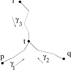
summed over all triples γ1\gamma_{1}, γ2\gamma_{2}, γ3\gamma_{3} consisting of an ascending path, γ1\gamma_{1}, from pp to tt, an ascending path, γ2\gamma_{2}, from qq to tt, and a descending path, γ3\gamma_{3}, from rr to tt. (See Figure 4.1.)

Refer to caption
Figure 4.1. Configuration of paths

Thus, in particular, if there exist no such configurations, cp​q​r=0c_{pqr}=0. Now suppose that the hypothesis of Theorem 1.6 is satisfied, i.e. σ\sigma is a self-indexing Morse function. Then we claim that

(4.13) ∫τp+​τq−=δp​q.\int\tau_{p}^{+}\tau_{q}^{-}=\delta_{pq}\;.

In fact if q∉Fpq\not\in F_{p} the supports of τp+\tau_{p}^{+} and τq−\tau_{q}^{-} are non-overlapping so (4.13) is automatically zero; and if q=pq=p, then the support of τp+​τq−\tau_{p}^{+}\tau_{q}^{-} consists of the single point pp and it is easy to verify that (4.13) is equal to one. Thus (4.13) is trivially true except when q∈Fpq\in F_{p} and q≠pq\neq p. In this case however, σq>σp\sigma_{q}>\sigma_{p} so

k=degree ​τp+​τq−=degree ​τp++degree ​τq−=d−σq+σp<dk=\text{degree }\tau_{p}^{+}\tau_{q}^{-}=\text{degree }\tau_{p}^{+}+\text{degree }\tau_{q}^{-}=d-\sigma_{q}+\sigma_{p}<d

so the integral (4.13) is zero just by degree considerations. Thus if we substitute the sum

∑cp​qs​τs+\sum c_{pq}^{s}\tau_{s}^{+}

for τp+​τq+\tau_{p}^{+}\tau_{q}^{+} in (1.2) we obtain for cp​qsc_{pq}^{s} the formula (1.13).

5. Examples

Each of the summands in (1.12) is a rational function: an element of the quotient field, Q⁡(𝔤∗)Q({\mathfrak{g}}^{*}); however, the sum itself is a polynomial, so the singularities in the individual summands are mysteriously cancelling each other out. We will discuss below a few simple examples in which one can see how some of these cancellations are happening.

5.1. Cancellations occuring in the individual terms

Suppose γ\gamma is a longest ascending path from pp to qq. Let e1,..,eme_{1},..,e_{m} be the edges of γ\gamma ordered so that t⁡(ek−1)=pk=i⁡(ek)t(e_{k-1})=p_{k}=i(e_{k}). Then eke_{k} is the only path joining pkp_{k} to pk+1p_{k+1}; hence the intersection numbers, ιek\iota_{e_{k}}, are all global intersection numbers of the form (4.8) and are in 𝕊⁡(𝔤∗){\mathbb{S}}({\mathfrak{g}}^{*}). Hence the factor

∏ιek\prod\iota_{e_{k}}

in the formula (1.12) is in 𝕊⁡(𝔤∗){\mathbb{S}}({\mathfrak{g}}^{*}). If, in addition, the Morse function ϕ\phi is self-indexing, this factor is a polynomial of degree zero, i.e. is just a constant.

5.2. Nearby paths

Suppose Γ\Gamma contains a totally geodesic subgraph of the form shown in Figure 5.1.

Refer to caption
Figure 5.1. Nearby paths

Let γ\gamma be the path consisting of the single edge, ee, joining pp to qq and let γ1\gamma_{1} be the path p→r→qp\to r\to q. Assume γ1\gamma_{1} is a longest path joining pp to qq and that σq=σp+2\sigma_{q}=\sigma_{p}+2. We claim that

E⁡(γ)+E⁡(γ1)=νqαe​αe′′.E(\gamma)+E(\gamma_{1})=\frac{\nu_{q}}{\alpha_{e}\alpha_{e^{\prime\prime}}}\;.
Proof.

We first note that

(5.1) αe=αe′+αe′′.\alpha_{e}=\alpha_{e^{\prime}}+\alpha_{e^{\prime\prime}}\;.

(This is a consequence of the compatibility conditions

−αe′′=αe′+c1​αeandαe′′=αe+c2​αe′-\alpha_{e^{\prime\prime}}=\alpha_{e^{\prime}}+c_{1}\alpha_{e}\quad\text{and}\quad\alpha_{e^{\prime\prime}}=\alpha_{e}+c_{2}\alpha_{e^{\prime}}

from which one concludes that c1=c2=−1c_{1}=c_{2}=-1.)

Let γ′\gamma^{\prime} be the path joining pp to rr and γ′′\gamma^{\prime\prime} the path joining rr to qq. By (4.2)

E⁡(γ)=νqαe⋅1ρe​(αe′′),E⁡(γ′)=−νrαe′,E⁡(γ′′)=−νqαe′′E(\gamma)=\frac{\nu_{q}}{\alpha_{e}}\cdot\frac{1}{\rho_{e}(\alpha_{e^{\prime\prime}})}\;,\quad E(\gamma^{\prime})=-\frac{\nu_{r}}{\alpha_{e^{\prime}}}\;,\quad E(\gamma^{\prime\prime})=-\frac{\nu_{q}}{\alpha_{e^{\prime\prime}}}

and by (4.9)

E⁡(γ1)=E⁡(γ′)νr⋅E⁡(γ′′)ρe′′​(αe′)​αe′.E(\gamma_{1})=\frac{E(\gamma^{\prime})}{\nu_{r}}\cdot\frac{E(\gamma^{\prime\prime})}{\rho_{e^{\prime\prime}}(\alpha_{e^{\prime}})}\alpha_{e^{\prime}}\;.

Hence

E⁡(γ1)=1νr​(−νrαe′)​(−νqαe′′)​αe′ρe′′​(αe′)=νqαe′′​ρe′′​(αe′).E(\gamma_{1})=\frac{1}{\nu_{r}}\Bigl(-\frac{\nu_{r}}{\alpha_{e^{\prime}}}\Bigr)\Bigl(-\frac{\nu_{q}}{\alpha_{e^{\prime\prime}}}\Bigr)\frac{\alpha_{e^{\prime}}}{\rho_{e^{\prime\prime}}(\alpha_{e^{\prime}})}=\frac{\nu_{q}}{\alpha_{e^{\prime\prime}}\rho_{e^{\prime\prime}}(\alpha_{e^{\prime}})}\;.

However, by (5.1), ρe′′​(αe′)=ρe′′​(αe−αe′′)=ρe′′​(αe)\rho_{e^{\prime\prime}}(\alpha_{e^{\prime}})=\rho_{e^{\prime\prime}}(\alpha_{e}-\alpha_{e^{\prime\prime}})=\rho_{e^{\prime\prime}}(\alpha_{e}); hence we can rewrite this as

E⁡(γ1)=νqαe′′​ρe′′​(αe);E(\gamma_{1})=\frac{\nu_{q}}{\alpha_{e^{\prime\prime}}\rho_{e^{\prime\prime}}(\alpha_{e})}\;;

so E⁡(γ)+E⁡(γ1)E(\gamma)+E(\gamma_{1}) is equal to the expression :

νq​(1αe​ρe​(αe′′)+1αe′′​ρe′′​(αe)).\nu_{q}\Bigl(\frac{1}{\alpha_{e}\rho_{e}(\alpha_{e}^{\prime\prime})}+\frac{1}{\alpha_{e^{\prime\prime}}\rho_{e^{\prime\prime}}(\alpha_{e})}\Bigr)\;.

However,

ρe​(αe′′)=−αe′′​(ξ)αe​(ξ)​ρe′′​(αe),\rho_{e}(\alpha_{e}^{\prime\prime})=-\frac{\alpha_{e^{\prime\prime}}(\xi)}{\alpha_{e}(\xi)}\rho_{e^{\prime\prime}}(\alpha_{e})\;,

so the term in parentheses can be rewritten

1αe​ρe​(αe′′)−\displaystyle\frac{1}{\alpha_{e}\rho_{e}(\alpha_{e^{\prime\prime}})}- αe′′​(ξ)αe​(ξ)⋅1αe′′​ρe​(αe′′)=1ρe​(αe′′)​(1αe−αe′′​(ξ)αe​(ξ)​1αe)=\displaystyle\frac{\alpha_{e^{\prime\prime}}(\xi)}{\alpha_{e}(\xi)}\cdot\frac{1}{\alpha_{e^{\prime\prime}}\rho_{e}(\alpha_{e^{\prime\prime}})}=\frac{1}{\rho_{e}(\alpha_{e^{\prime\prime}})}\Bigl(\frac{1}{\alpha_{e}}-\frac{\alpha_{e^{\prime\prime}}(\xi)}{\alpha_{e}(\xi)}\frac{1}{\alpha_{e}}\Bigr)=
=\displaystyle= 1ρe​(αe′′)⋅αe′′−(αe′′​(ξ)/αe​(ξ))​αeαe​αe′′=1αe​αe′′.∎\displaystyle\frac{1}{\rho_{e}(\alpha_{e^{\prime\prime}})}\cdot\frac{\alpha_{e^{\prime\prime}}-(\alpha_{e^{\prime\prime}}(\xi)/\alpha_{e}(\xi))\alpha_{e}}{\alpha_{e}\alpha_{e^{\prime\prime}}}=\frac{1}{\alpha_{e}\alpha_{e}^{\prime\prime}}\;.\qed

5.3. The flag variety G=S​L​(n,ℂ)/BG=SL(n,{\mathbb{C}})/B.

Graph theoretically, the flag variety S​L​(n,ℂ)/BSL(n,{\mathbb{C}})/B is the permutahedron: a Cayley graph associated with the Weyl group of S​L​(n,ℂ)SL(n,{\mathbb{C}}), the symmetric group SnS_{n}. Each vertex of this graph corresponds to a permutation π∈Sn\pi\in S_{n}, and two permutations π\pi and π′\pi^{\prime}, are adjacent in Γ\Gamma if and only if there exists a transposition τi​j\tau_{ij}, 1≤i<j≤n1\leq i<j\leq n with π′=π​τi​j\pi^{\prime}=\pi\tau_{ij}. Moreover, if ee is the edge joining π\pi to π​τi​j\pi\tau_{ij}, the weight labeling ee is

αe={ϵj−ϵi, if ​π​(j)>π⁡(i)ϵi−ϵj, if ​π​(j)<π⁡(i),\alpha_{e}=\begin{cases}\epsilon_{j}-\epsilon_{i},&\mbox{ if }\pi(j)>\pi(i)\\ \epsilon_{i}-\epsilon_{j},&\mbox{ if }\pi(j)<\pi(i),\end{cases}

where ϵ1,..,ϵn\epsilon_{1},..,\epsilon_{n} is the standard basis vectors of the lattice ℤn{\mathbb{Z}}^{n}. The connection θe\theta_{e} along this edge is given by

θπ,π​τ​(π,π​τ′)=(π​τ,π​τ′​τ).\theta_{\pi,\pi\tau}(\pi,\pi\tau^{\prime})=(\pi\tau,\pi\tau^{\prime}\tau)\;.

If ξ=(ξ1,…,ξn)∈𝒫\xi=(\xi_{1},...,\xi_{n})\in{\mathcal{P}}, with ξ1<…,ξn\xi_{1}<...,\xi_{n}, then the function

ϕ:VΓ→ℤ,ϕ⁡(π)=length​(π)\phi:V_{\Gamma}\to{\mathbb{Z}}\;,\qquad\phi(\pi)=\mbox{length}(\pi)

is a self-indexing ξ\xi-compatible Morse function on Γ\Gamma.

The permutahedron is a bi-partite graph, with the two sets of vertices corresponding to even, respective odd permutations. In the special case n=3n=3, this graph is a complete bi-partite graph, and the corresponding labeling is shown in Figure 5.2.

Refer to caption
Figure 5.2. The flag variety

Here α1=ϵ2−ϵ1\alpha_{1}=\epsilon_{2}-\epsilon_{1} and α2=ϵ3−ϵ2\alpha_{2}=\epsilon_{3}-\epsilon_{2}, and we have used the notation (231)(231) for the cycle 1→2→3→11\to 2\to 3\to 1.

The quantities Θp​q\Theta_{pq} given by (4.6) are all equal to 1, with the exception of Θ1,(13)\Theta_{1,(13)}, which is

Θ1,(13)=1ρα1+α2​(α1​α2)=−(α1​(ξ)+α2​(ξ))2(α2​(ξ)​α1−α1​(ξ)​α2)2\Theta_{1,(13)}=\frac{1}{\rho_{\alpha_{1}+\alpha_{2}}(\alpha_{1}\alpha_{2})}=-\frac{(\alpha_{1}(\xi)+\alpha_{2}(\xi))^{2}}{(\alpha_{2}(\xi)\alpha_{1}-\alpha_{1}(\xi)\alpha_{2})^{2}}

There are two ascending paths from (12) to (13), namely

γ1:(12)→(231)→(13) and γ2:(12)→(312)→(13)\gamma_{1}:(12)\to(231)\to(13)\quad\text{ and }\quad\gamma_{2}:(12)\to(312)\to(13)

and their contributions to τ(12)​(13)\tau_{(12)}(13) are

E⁡(γ1)\displaystyle E(\gamma_{1}) =−α1α2(α1+α2)⋅1α1⋅1ρα1​(α1+α2)=α1​(ξ)​α2​(α1+α2)α2​(ξ)​α1−α1​(ξ)​α2\displaystyle=-\alpha_{1}\alpha_{2}(\alpha_{1}+\alpha_{2})\cdot\frac{1}{\alpha_{1}}\cdot\frac{1}{\rho_{\alpha_{1}}(\alpha_{1}+\alpha_{2})}=\frac{\alpha_{1}(\xi)\alpha_{2}(\alpha_{1}+\alpha_{2})}{\alpha_{2}(\xi)\alpha_{1}-\alpha_{1}(\xi)\alpha_{2}}
and
E⁡(γ2)\displaystyle E(\gamma_{2}) =−α1α2(α1+α2)⋅1α2⋅1ρα2​(α1+α2)=−α2​(ξ)​α1​(α1+α2)α2​(ξ)​α1−α1​(ξ)​α2,\displaystyle=-\alpha_{1}\alpha_{2}(\alpha_{1}+\alpha_{2})\cdot\frac{1}{\alpha_{2}}\cdot\frac{1}{\rho_{\alpha_{2}}(\alpha_{1}+\alpha_{2})}=-\frac{\alpha_{2}(\xi)\alpha_{1}(\alpha_{1}+\alpha_{2})}{\alpha_{2}(\xi)\alpha_{1}-\alpha_{1}(\xi)\alpha_{2}}\;,

so

τ(12)​(13)=E⁡(γ1)+E⁡(γ2)=−α1−α2.\tau_{(12)}(13)=E(\gamma_{1})+E(\gamma_{2})=-\alpha_{1}-\alpha_{2}\;.

The other classes can be computed similarly and are given by

τ1\tau_{1} τ(12)\tau_{(12)} τ(23)\tau_{(23)} τ(231)\tau_{(231)} τ(312)\tau_{(312)} τ(13)\tau_{(13)}
1 1 0 0 0 0 0
(12) 1 −α1-\alpha_{1} 0 0 0 0
(23) 1 0 −α2-\alpha_{2} 0 0 0
(231) 1 −α1−α2-\alpha_{1}-\alpha_{2} −α2-\alpha_{2} α2​(α1+α2)\alpha_{2}(\alpha_{1}+\alpha_{2}) 0 0
(312) 1 −α1-\alpha_{1} −α1−α2-\alpha_{1}-\alpha_{2} 0 α1​(α1+α2)\alpha_{1}(\alpha_{1}+\alpha_{2}) 0
(13) 1 −α1−α2-\alpha_{1}-\alpha_{2} −α1−α2-\alpha_{1}-\alpha_{2} α2​(α1+α2)\alpha_{2}(\alpha_{1}+\alpha_{2}) α1​(α1+α2)\alpha_{1}(\alpha_{1}+\alpha_{2}) −α1​α2​(α1+α2)-\alpha_{1}\alpha_{2}(\alpha_{1}+\alpha_{2})

5.4. The zero-dimensional Thom class

Suppose the graph Γ\Gamma is connected and hence has a unique vertex, p0p_{0}, of index zero. Then the Thom class, τp0\tau_{p_{0}}, is the unique generator of H0​(Γ,α)H^{0}(\Gamma,\alpha), with τp0​(p0)=1\tau_{p_{0}}(p_{0})=1. Thus

(5.2) τp0​(p)=1\tau_{p_{0}}(p)=1

for all vertices pp. We will show how to deduce (5.2) from (1.11). Choose the constants, cc and c′c^{\prime}, in (3.21), so that p0p_{0} is the only vertex with ϕ⁡(p0)<c\phi(p_{0})<c and such that ϕ⁡(p)\phi(p) is the smallest critical value of ϕ\phi greater that c′c^{\prime}. By the Markov property of the map (3.22)

1=∑w∈VcQ⁡(v,w)1=\sum_{w\in V_{c}}Q(v,w)

for every vertex v∈Vc′v\in V_{c^{\prime}}. In particular let

Ep−={ei,i=1,..,r}E_{p}^{-}=\{e_{i}\;,\;i=1,..,r\}

and let vi∈Vc′v_{i}\in V_{c^{\prime}} be the vertex at which eie_{i} intersects Γc′\Gamma_{c^{\prime}}. Then by (3.28)

τp0​(p)=∑i=1rQ⁡(ei)​∑wQ⁡(vi,w)=∑Q⁡(ei)\tau_{p_{0}}(p)=\sum_{i=1}^{r}Q(e_{i})\sum_{w}Q(v_{i},w)=\sum Q(e_{i})

and by (3.26)

τp0​(p)=∑i=1r∏j≠iαejαej−(αej​(ξ)/αei​(ξ))​αei.\tau_{p_{0}}(p)=\sum_{i=1}^{r}\prod_{j\neq i}\frac{\alpha_{e_{j}}}{\alpha_{e_{j}}-(\alpha_{e_{j}}(\xi)/\alpha_{e_{i}(\xi)})\alpha_{e_{i}}}\;.

Letting

xi=−1αei​(ξ)​αeix_{i}=-\frac{1}{\alpha_{e_{i}}(\xi)}\alpha_{e_{i}}

this becomes

∑i=1r∏j≠i−xjxi−xj,,\sum_{i=1}^{r}\prod_{j\neq i}\frac{-x_{j}}{x_{i}-x_{j}},\;,

which is equal to 1 by (3.11). Thus τp0​(p)=1\tau_{p_{0}}(p)=1.

5.5. The (n−1)(n-1)-dimensional projective space

Graph theoretically this is just the complete graph, Δ\Delta, on nn vertices. Let us denote these vertices by p1,..,pnp_{1},..,p_{n} and as in Section 3 assign to the edge, ee, joining pip_{i} to pjp_{j}, the weight

αe=xi−xj.\alpha_{e}=x_{i}-x_{j}\;.

(As we pointed out in Section 3 this defines an axial function on Δ\Delta.) Let ξ\xi be an nn-tuple of real numbers with ξ1>ξ2>…>ξn\xi_{1}>\xi_{2}>...>\xi_{n} and orient the edges of Δ\Delta by decreeing that an edge, ee, is ascending if αe​(ξ)>0\alpha_{e}(\xi)>0. With this orientation, the function mapping pip_{i} to ii is a ξ\xi-compatible Morse function. Lets compute the Thom class, τpi\tau_{p_{i}}. If i=1i=1, we get from the computation above

τp1​(p)=1\tau_{p_{1}}(p)=1

for all vertices pp. If i>1i>1, we can regard the vertices pi,pi+1p_{i},p_{i+1}, … , pnp_{n} as the vertices of a complete graph, Δ′\Delta^{\prime}, having the same axial function as above. Consider the sum

(5.3) ∑E⁡(γ)\sum E(\gamma)

over all ascending paths joining p=pip=p_{i} to q=pjq=p_{j}, where j>ij>i. The individual summands can be written in the form

νqνq′​E′​(γ),\frac{\nu_{q}}{\nu_{q}^{\prime}}E^{\prime}(\gamma)\;,

where by (1.12)

E′​(γ)=(−1)m​νq′​ιe1αm​∏k=2mιekαk−1−αkE^{\prime}(\gamma)=(-1)^{m}\nu_{q}^{\prime}\frac{\iota_{e_{1}}}{\alpha_{m}}\prod^{m}_{k=2}\frac{\iota_{e_{k}}}{\alpha_{k-1}-\alpha_{k}}

and νq′\nu_{q}^{\prime} is the product

∏αe′′\prod{{}^{\prime}}{}\alpha_{e^{\prime}}

over all descending edge, e′∈Eq−e^{\prime}\in E_{q}^{-}, which join qq to vertices in Δ′\Delta^{\prime}. Then (5.3) becomes

νqνq′​(∑E′​(γ)).\frac{\nu_{q}}{\nu_{q}^{\prime}}\Bigl(\sum E^{\prime}(\gamma)\Bigr)\;.

However, by (1.11) the expression in parentheses computes the zeroth Thom class of the subgraph Δ′\Delta^{\prime}, at qq, and hence is equal to one. Thus

τpi​(q)=νqνq′=∏αe′′′,\tau_{p_{i}}(q)=\frac{\nu_{q}}{\nu_{q}^{\prime}}=\prod{{}^{\prime}}{}\alpha_{e^{\prime\prime}}\;,

where ∏′\prod^{\prime} is the product over all the edges e′′e^{\prime\prime} of Δ\Delta, which join qq to the vertices pkp_{k}, k=1,..,i−1k=1,..,i-1.

References

  • [AB] M. F. Atiyah and R. Bott, The moment map and equivariant cohomology, Topology 23 (1984), 1-28.
  • [BV] N. Berline and M. Vergne, Classes caractéristiques équivariantes, C.R. Acad. Sci., Paris 295 (1982), 539-541.
  • [BH] S. Billey and M. Haiman, Schubert polynomials for the classical group, J. Amer.Math.Soc. 8 (1995), no. 2, 443-482.
  • [Bi] S. Billey, Kostant polynomials and the cohomology ring for G/BG/B, Duke Math. J. 96 (1999), no. 1, 205-224.
  • [GKM] M. Goresky, R. Kottwitz and R. MacPherson, Equivariant cohomology, Koszul duality and the localization theorem, Invent. Math. 131 (1998), no. 1, 25-83.
  • [GZ1] V. Guillemin and C. Zara, Equivariant de Rham theory and graphs, Asian J. of Math. 3 (1999), no. 1, 49-76.
  • [GZ2] V. Guillemin and C. Zara, One-skeleta, Betti numbers and Equivariant Cohomology, math.DG/9903051, to appear in Duke Math. J.
  • [GZ3] V. Guillemin and C. Zara, Morse Theory on Graphs, math.CO/0007161
  • [Kn] A. Knutson, Descent cycling in Schubert calculus, in preparation.
  • [Ko] M. Kogan, Schubert geometry of flag varieties and Gelfand-Cetlin Theory, Ph.D. thesis, MIT 2000.
  • [Za] C. Zara, One-skeleta and the equivariant cohomology of GKM manifolds, Ph.D. thesis, MIT 2000.