Neural Stabilization/Excitation Control of a High-Order Power System by Adaptive Feedback LinearizationThanks: This work was supported by the Natural Sciences and Engineering Research Council of Canada via a research grant.

The differential geometric technique of state feedback linearization has been explored over the past two decades for the purpose of power system control (see, for instance, [2], [17], [4], [6]). The main idea is to perform a co-ordinate transformation of the nonlinear state space system equations and define a new control input so that in the new co-ordinates, the nonlinearities in the plant are either wholly or partially masked. This formulation may result in linearizations which are valid for large practical operating points of the system, as opposed to a local Jacobian linearization about an operating point.

Feedback linearization has been applied to the control of power systems represented by the state-space single machine/infinite bus model in two main ways. The input-state feedback linearization approach is formulated such that the system state becomes a linear function of a new control input and a new state, while the output (for our purposes, the terminal voltage) is still a nonlinear function, e.g. see [17]. Although this works well for designing stabilizing controllers, the nonlinearities in the output map make it very difficult to achieve good tracking of reference voltage signals. An alternative to this approach is the input-output feedback linearization in which the terminal voltage becomes a linear function of a new control input, e.g. see [2], [3], [4]. Due to the mathematical complexity of the nonlinear state-space model representing the high-order single machine/infinite bus power system (a $7th$ order model), a simplified $3rd$ order model is used in [2], [3]. An excitation controller/stabilizer is then designed and tested using the high order model of the plant. The effects of the unmodelled system dynamics and possible shifts in parameters of the plant raise some questions on the effectiveness of the controller. An inherent drawback of the feedback linearization approach is the non-robustness due to the need for exact knowledge, both in terms of the structure and parameters, of the model of the power system. Adaptive control has been used to compensate for parameter variation in a framework that allows the controller to learn the nonlinearities on-line [12]. However, this assumes that the nonlinearities can be parameterized linearly in some unknown parameters [12], [13]. Some power system stabilizers based on adaptive control design techniques have been shown to increase the operating range over which they can provide good control as well as exhibit robustness to parameterized system disturbances [10].

This paper presents a design which addresses these problems by working directly with the more accurate $7th$ order model of the power system. The nonlinear dynamical system is modelled using multilayer neural networks made of sigmoid type nonlinearities and adjustable weights which are nonlinearly parameterized. The flexibility provided by the nonlinear parameterization allows for a more realistic representation of the underlying nonlinear power system model. Power system controller designs using neural networks of various configurations exist in the literature and are reported in works like [1]. Neural adaptive control of feedback linearizable nonlinear systems was first proposed in [7] and extensively analyzed in [8]. In these references, the networks were trained using the backpropagation algorithm [5]; the nonlinear function approximation capability of neural networks (see [14]) was exploited to model the plant in order to determine an appropriate feedback linearizing control. However, the approach used in [7], [8] provides no clear way of specifying closed loop dynamics. In this work the neural network identifier is trained in batch form and adapted using the Levenberg-Marquardt optimization (as in [15]) rather than using standard backpropagation. Also, the whole control problem is formulated such that tracking dynamics can be user-specified by approprately assigning closed loop system poles. Weight adaptation based on nonlinear optimization is attractive here because it significantly corrects some of the defects of standard backpropagation, most importantly slow rate of convergence. In this framework, the trained neural networks give an on-line estimate of the parameters of the power system at every sampling instant which are then used to calculate the feedback linearizing control law. The controller is designed to provide reference tracking (with bounded state), damping of power angle oscillations and tolerate variations in the plant parameters. It may also be adapted on-line.

This paper is organized as follows: Section 2 presents the state-space synchronous machine/infinte bus power system model. The system relative degree and minimum phase properties, important for feedback linearization to be successfully applied, are also discussed. The class of systems to which this model belongs and which motivates the choice of a neural identifier is determined. Section 3 focuses on the neural modelling of the power system while Section 4 presents a systematic design of the proposed excitation controller/power system stabilizer. Finally, simulation results are presented and discussed in Section 5, followed by some concluding remarks.

The model used is developed in [16] (p. 54ff). It yields a Park’s 7th order nonlinear time-invariant, state-space description of the synchronous generator/infinite bus system. This is connected through a balanced pair of transmission lines to a power system modelled simply as one of infinitely large ability to supply and absorb power at a set voltage level, i.e. an infinite bus system. The system is depicted in Fig. 1.

State variables for this generator/infinite bus set-up are selected as follows:

• •

  $\delta(x_{1})$ - power angle

• •

  $\omega(x_{2})$ - power angle derivative

• •

  $\lambda_{d}(x_{3})$ - d-axis flux linkage

• •

  $\lambda_{q}(x_{4})$ - q-axis flux linkage

• •

  $\lambda_{f}(x_{5})$ - field flux linkage

• •

  $\lambda_{k_{d}}(x_{6})$ - damper d-axis flux linkage

• •

  $\lambda_{k_{q}}(x_{7})$ - damper q-axis flux linkage

The system model is given by

	$\displaystyle\dot{\delta}$	$\displaystyle=$	$\displaystyle\omega$
	$\displaystyle\dot{\omega}$	$\displaystyle=$	$\displaystyle\frac{\omega_{b}}{2H}[P_{m}-P_{e}(\delta,\lambda_{d},\lambda_{q})-D\omega]$		(1)
	$\displaystyle\dot{\lambda}$	$\displaystyle=$	$\displaystyle\omega_{b}\left([RL^{-1}+Z]\lambda+[v_{d}\;v_{q}\;v_{f}\;0\;0]^{T}\right)$

where $\lambda:=[\lambda_{d}\;\lambda_{q}\;\lambda_{f}\;\lambda_{k_{d}}\;\lambda_{k_{q}}]^{T}$, are the per unit flux linkages, R := $diag\;[r_{s}\;r_{s}\;-r_{f}\;-r_{k_{d}}\;-r_{k_{q}}],$ are per unit resistances. $H$ is the inertia constant, $D$ encapsulates the damping in the system,

$\displaystyle L:=\left[\begin{array}[]{ccccc}-L_{d}&0&L_{ad}&L_{ad}&0\\ 0&-L_{q}&0&0&L_{aq}\\ -L_{ad}&0&L_{f}&L_{fk_{d}}&0\\ -L_{ad}&0&L_{fk_{d}}&L_{k_{d}}&0\\ 0&-L_{aq}&0&0&L_{k_{q}}\end{array}\right]$

are inductances, and

$\displaystyle Z:=\left[\begin{array}[]{rcccc}0&1&0&0&0\\ -1&0&0&0&0\\ 0&0&0&0&0\\ 0&0&0&0&0\\ 0&0&0&0&0\end{array}\right]_{.}$

As shown in Fig. 1, the control input ($u$) is the field voltage $v_{f}$ and the output to be controlled ($y$) is the generator terminal voltage $v_{t}$ given by

$\displaystyle y=v_{t}=h(\delta,\lambda_{d},\lambda_{q})=\sqrt{v^{2}_{d}+v^{2}_{q}}$

where

	$\displaystyle v_{d}$	$\displaystyle=$	$\displaystyle r_{11}I_{d}-x_{11}I_{q}+v_{\infty}[Acos(\pi/2-\delta)+Bsin(\pi/2-\delta)]$
	$\displaystyle v_{q}$	$\displaystyle=$	$\displaystyle r_{11}I_{q}-x_{11}I_{d}-v_{\infty}[Bcos(\pi/2-\delta)-Asin(\pi/2-\delta)]_{;}$

the variables are described in [16] and [3]. $A,\;B$ are constant matrices having values depending on physical parameters of the power system, $v_{\infty}$ is the voltage of the infinite bus, $I_{d,q}$ are $d-$ and $q-$ axis currents, $r_{11}$, $x_{11}$ are components of transmission line resistance and reactance (see [16]). The system model (1) belongs to the class of control affine nonlinear systems of the form

	$\displaystyle\dot{x}$	$\displaystyle=$	$\displaystyle f(x)+g(x)\cdot u$		(4)
	$\displaystyle y$	$\displaystyle=$	$\displaystyle h(x).$

Here $f$, $g$ are smooth functions; the state $x\in\mathbb{Re}^{n}$, input $u\in\mathbb{Re}$ and output $y\in\mathbb{Re}$. The relative degree and minimum phase properties of this system are examined next.

The relative degree of the power system (1) may be obtained by differentiating $y$ (i.e. $v_{t}$) until $u$ ($v_{f}$) appears. This is achieved by computing the Lie derivatives (see [9]) of the system.

	$\displaystyle L_{f}h$	$\displaystyle=$	$\displaystyle\nabla h\dot{x}$
		$\displaystyle=$	$\displaystyle\frac{dh}{dx_{1}}\dot{x}_{1}+\ldots+\frac{dh}{dx_{5}}\dot{x}_{5}+\ldots+\frac{dh}{dx_{7}}\dot{x}_{7}$

Observe that $v_{f}$ appears explicitly in the expression for $\dot{x}_{5}(\dot{\lambda}_{f})$ in (1). Therefore the output need only be differentiated once before the control input $v_{f}$ appears, i.e. the relative degree is 1. It is easy to show that the system (1) is nominally minimum phase over the practical operating region by linearizing the system at various operating points in the state-space and verifying left half plane zeros (see Appendix B in [18]).

From the relative degree and minimum phase properties, the identification model proposed for the system will be the single-input single-output relative-degree-one nonlinear discrete-time system

	$\displaystyle y[k+1]$	$\displaystyle=$	$\displaystyle f[y(k),\ldots,y(k-n+1),\;u(k-1),\ldots,u(k-m)]\;+$		(5)
			$\displaystyle g[y(k),\ldots,y(k-n+1),\;u(k-1),\ldots,u(k-m)]\cdot u(k)$

where $y$ is the output, $u$ is the input, $f$ and $g$ are assumed smooth and the system is assumed minimum phase. For the $7^{th}$-order power system with relative degree 1, n = 7, m = 6.

The first stage in the controller design is to identify the synchronous machine/infinite bus dynamical model using the structure (5). The set-up to do so is shown in Fig. 2. $TDLs$ are tapped delay lines used to implement the regressor structure for both networks.

NN-1 and NN-2 are feedforward neural networks whose input vector consists of present output and delayed inputs and outputs. They are used to predict the next output $y(k+1)$. NN-1 has one hidden layer made up of a total of $p$ neurons with hyperbolic tangent tanh activation function and an output layer of one neuron with linear activation function. NN-2 has $q$ tanh hidden layer neurons and one output neuron. All weights are initialized randomly and contain biases.

A training set is generated by exciting the plant with a variety of input signals $u$ (of appropriate range) and measuring the output $y$. That is, let $Z^{N}=\{[u(k),y(k)]|k=1,\ldots,N\}$, represent the training data pairs and N be the total number of data sets. The estimate of the plant output given by the neural nets is

$$\hat{y}[k+1]=\hat{f}[z(k),{\bf w}]+\hat{g}[z(k),{\bf v}]\cdot u(k)$$

(6)

where

	$\displaystyle\hat{f}(z(k),w)$	$\displaystyle=$	$\displaystyle\sum^{p}_{i=1}w_{i}\>\tanh\left(\sum^{m+n}_{j=1}\>w_{ij}z_{j}+b_{i}\right)+b$
	$\displaystyle\hat{g}(z(k),v)$	$\displaystyle=$	$\displaystyle\sum^{p}_{i=1}v_{i}\>\tanh\left(\sum^{m+n}_{j=1}\>v_{ij}z_{j}+a_{i}\right)+a;$

$(w,b)$ and $(v,a)$ are weights and biases respectively for the $\hat{f}(\cdot)$ and $\hat{g}(\cdot)$ networks. Let the set of possible weights be $\hat{\Theta}$ and define the cost function ${\bf J}$ as the mean square error in predicting the plant output. That is,

$$J_{N}(\Theta,Z^{N})=\frac{1}{2N}\sum^{N}_{k=1}\left[y(k+1)-\hat{y}(k+1|\Theta)\right]^{T}\left[y(k+1)-\hat{y}(k+1|\Theta)\right].$$

(7)

The optimal weights are determined by solving

$$\hat{\Theta}=arg\;\min_{\Theta}\;J_{N}(\Theta,Z^{N})$$

Let the weight update rule toward achieving the optimal choice be given by

$$\Theta_{k+1}=\Theta_{k}+\rho_{k}S_{k}$$

where $\Theta_{k}$ is the current iterate of the set of weights, $\rho_{k}$ is the step size and $S_{k}$ is the search direction.

For identification purposes, the weight update is done in batch form using the Levenberg-Marquardt optimization as described in [15]. When the cost function is minimized to an acceptable level, weight adaptation is discontinued and the neural model is validated on the training data set and subsequently cross-validated on other sets of data not in the original training set. Simulation results are provided which show the effectiveness of the proposed identification technique.

Recall that the power system is modelled by the SISO discrete time system:

	$\displaystyle y[k+1]$	$\displaystyle=$	$\displaystyle f[y(k),\ldots,y(k-n+1),\;u(k-1),\ldots,u(k-m)]\;+$		(8)
			$\displaystyle g[y(k),\ldots,y(k-n+1),\;u(k-1),\ldots,u(k-m)]\cdot u(k)$

and estimated by the neural model:

	$\displaystyle\hat{y}[k+1]$	$\displaystyle=$	$\displaystyle\hat{f}[y(k),\ldots,y(k-n+1),\;u(k-1),\ldots,u(k-m)]\;+$		(9)
			$\displaystyle\hat{g}[y(k),\ldots,y(k-n+1),\;u(k-1),\ldots,u(k-m)]\cdot u(k)$

A simple pole-placement controller is proposed to allow the tracking dynamics to be specified by appropriately placing closed-loop poles at stable locations. Let the reference signal to be tracked be given by $r(k)$.

To facilitate the discussion, a state-space form of the system (8) is constructed by choosing state variables as follows:

	$\displaystyle z_{11}(k)$	$\displaystyle=$	$\displaystyle y(k-n+1)$
	$\displaystyle z_{1n}(k)$	$\displaystyle=$	$\displaystyle y(k)$
	$\displaystyle z_{21}(k)$	$\displaystyle=$	$\displaystyle u(k-m)$
	$\displaystyle z_{2m}(k)$	$\displaystyle=$	$\displaystyle u(k-1)$

and we subsequently define

$\displaystyle{\bf z}$

$\displaystyle=$

$\displaystyle\left[\begin{array}[]{c}{\bf z}_{1}\\ {\bf z}_{2}\end{array}\right]\;=\;\left[\begin{array}[]{c}z_{11}\\ \vdots\\ z_{1n}\\ -\\ z_{21}\\ \vdots\\ z_{2m}\end{array}\right]_{.}$

This leads to the state-space model:

	$\displaystyle z_{11}(k+1)$	$\displaystyle=$	$\displaystyle z_{12}(k)$
	$\displaystyle z_{1n}(k+1)$	$\displaystyle=$	$\displaystyle f[{\bf z}(k)]+g[{\bf z}(k)]\cdot u(k)=y[k+1]$		(11)
	$\displaystyle z_{21}(k+1)$	$\displaystyle=$	$\displaystyle z_{22}(k)$
	$\displaystyle z_{2m}(k+1)$	$\displaystyle=$	$\displaystyle u(k)$
	$\displaystyle y(k)$	$\displaystyle=$	$\displaystyle z_{1n}(k)$

Now we define a new control input $\tilde{u}$ and set

$\displaystyle u(k)$

$\displaystyle=$

$\displaystyle\frac{1}{g[{\bf z}(k)]}\left[-f[{\bf z}(k)]+\tilde{u}(k)\right];$

(12)

observe that this results in input-output closed loop dynamics of

$\displaystyle y[k+1]$

$\displaystyle=$

$\displaystyle\tilde{u}(k)$

Now we address the primary control objective of tracking a constant reference voltage $r=v_{t}$. This motivates the choice of the feedback control $\tilde{u}(k)$ as

$\displaystyle\tilde{u}(k)=K_{1}r(k)-\left[C_{p-1}y(k)+C_{p-2}y(k-1)+\cdots+C_{0}y(k-p+1)\right]$

(13)

with $p\in\mathbb{Z}^{+}$ and $C_{i}\in\mathbb{R}$. Hence,

$\displaystyle y[k+1]+C_{p-1}y(k)+C_{p-2}y(k-1)+\cdots+C_{0}y(k-p+1)$

$\displaystyle=$

$\displaystyle K_{1}r(k).$

Therefore the transfer function between the reference and $y$ is given by

$\displaystyle\frac{V_{t}[z]}{V_{ref}[z]}$

$\displaystyle=$

$\displaystyle\frac{Y[z]}{R[z]}=\frac{K_{1}}{z^{p}+C_{p-1}z^{p-1}+\cdots+C_{1}z+C_{0}}\;=:\;\frac{K_{1}}{Q(z)}.$

(14)

Closed loop poles for the system can be assigned by selecting constants $C_{i}$’s so that the zeros of the characteristic polynomial $Q(z)$ are all in the unit circle.

Some assumptions made on the system and a discussion of the stability of this kind of control scheme can be found in [18]. Specifically, it is shown therein that the approach used here is a more general form of that extensively analyzed in [8].

Now we rewrite the plant in the input-output form as

$$y(k+1)\;=\;f[{\bf z}(k)]+g[{\bf z}(k)]\cdot u(k)$$

(15)

The plant (15) is thus modelled by the neural networks as:

$$\hat{y}(k+1)\;=\;\hat{f}[{\bf z}(k),{\bf w}]+\hat{g}[{\bf z}(k),{\bf v}]\cdot u(k)$$

(16)

For the three-layer neural networks used in the identification stage, with total hidden neurons $p$ and $q$ respectively and weights/biases $(w_{i},\;\hat{w}_{i}\in{\bf w})$ and $(v_{i},\;\hat{v}_{i}\in{\bf v})$ , the functions $\hat{f}(\cdot,\cdot)$ and $\hat{g}(\cdot,\cdot)$ can be expressed as

$$\hat{f}[{\bf z}(k),{\bf w}]=\sum^{p}_{i=1}w_{i}\>\tanh\left(\sum^{m+n}_{j=1}\>w_{ij}x_{j}+\hat{w}_{i}\right)$$

(17)

and

$$\hat{g}[{\bf z}(k),{\bf v}]=\sum^{p}_{i=1}v_{i}\>\tanh\left(\sum^{m+n}_{j=1}\>v_{ij}x_{j}+\hat{v}_{i}\right)$$

(18)

Funahashi’s theorem [14] says that we can approximate $f$ and $g$ as close as we like by a suitably parameterized neural network. It is not presently known how to choose the number of neurons given a desired error tolerance. However, the typical approach is to choose a configuration and try to obtain good weights/biases by trying to solve a nonlinear optimization problem. If the approximation is poor, the configuration is adjusted and repeated. This will be accomplished via an “off-line” training phase using the Levenberg-Marquardt algorithm (as discussed in Section 3), to obtain initial estimates of $\hat{f}$ and $\hat{g}$.

Now, we focus on the on-line phase, in which the controller is applied to the system. An additional constraint to consider is the need to ensure that $\hat{g}$ remains nonzero due to the fact that the controller incorporates a division by $\hat{g}$ as shown in (19).

Let ${\bf w}(k)$ and ${\bf v}(k)$ denote the estimates of ${\bf w}$ and ${\bf v}$ at sampling instant $k$. The control input $u(k)$ is then given as:

Control Law:

$$\vskip 28.45274ptu(k)\;=\;\frac{-\hat{f}[{\bf z}(k),{\bf w}(k)]+\tilde{u}(k)}{\hat{g}[{\bf z}(k),{\bf v}(k)]}$$

(19)

with $\tilde{u}(k)$ as previously defined in (13). The control $u(k)$ is applied to both the plant and the neural network model; the network weights are updated using the error between the plant output and the output predicted by the neural model. At each sampling instant $k$, the estimated plant output is given by

$$\hat{y}^{*}(k+1)\;=\;\hat{f}[{\bf z}(k),{\bf w}(k)]\;+\;\hat{g}[{\bf z}(k),{\bf v}(k)]\cdot u(k)$$

(20)

The error associated with this estimate $\{e^{*}(k+1)\}$ is defined as

$$e^{*}(k+1)\;=\;\hat{y}^{*}(k+1)-y(k+1)$$

(21)

This error (together with a deadzone adaptation) will be used in the weight update rule described next. A deadzone is an absolute lower limit on the adaptation error below which no adaptation should be done. That is to say, before the weights are adapted at each sampling instant, the plant output error $e^{*}(k+1)$ is compared with the dead zone radius $d_{0}$. If $\left|e^{*}(k+1)\right|\leq d_{0}$, no adaptation is done, otherwise the adaptation is done using an error adaptation rule based on the deadzone $D(e)$ given by

$\displaystyle D(e)=\left\{\begin{array}[]{lcl}0&if&\left|e\right|\leq d_{0}\\ e-d_{0}&if&e>d_{0}\\ e+d_{0}&if&e<-d_{0}\\ \end{array}\right.$

which ensures that the constraint of nonzero $\hat{g}$ holds. In order to implement the weight update rule, first define the set of network weights $\Theta$ as

$$\Theta\;=\;\left[\begin{array}[]{cc}{\bf w}\\ {\bf v}\end{array}\right]$$

and the Jacobian to be computed at each time step by

	$\displaystyle{\bf J}_{k}$	$\displaystyle=$	$\displaystyle\left[\left.\frac{\partial\hat{y}^{*}(k+1)}{\partial\Theta}\right|_{\Theta(k)}\right]^{{}^{\prime}}$
		$\displaystyle=$	$\displaystyle\left[\begin{array}[]{c}\left(\left.\frac{\partial\hat{f}[{\bf z}(k),{\bf w}]}{\partial{\bf w}}\right|_{{\bf w(k)}}\right)^{{}^{\prime}}\\ \left(\left.\frac{\partial\hat{g}[{\bf z}(k),{\bf v}]}{\partial{\bf v}}\right|_{{\bf v(k)}}\right)^{{}^{\prime}}\cdot u(k)\end{array}\right]_{.}$

This Jacobian can be calculated using the backpropagation algorithm [5] at the end of each iteration, since the variable $\hat{y}^{*}(k+1)$ is the output of the neural networks, and is available for use [8].

Adaptation Rule:

$$\Theta(k+1)\;=\;\Theta(k)-\frac{1}{(1+{\bf J}^{\prime}_{k}{\bf J}_{k})}D\left[e^{*}(k+1)\right]{\bf J}_{k}$$

(29)

Power system stabilizer: The power system stabilizer adds damping to the generator rotor angle oscillations by modulating its excitation using auxiliary stabilizing signal(s). In order to accomplish this, the stabilizer should be desgined to produce a component of electrical torque in phase with the rotor speed deviations. For the machine model being used, the signal of choice for modulating the excitation is the rotor angle derivative $\dot{\delta}$. This requires that the linearizing control law (12) be modified to introduce a torque component which damps out the oscillations of the rotor angle. The new control law is given by

$$u(k)=\frac{\tilde{u}(k)-\hat{f}(\cdot)}{\hat{g}(\cdot)}+K_{pss}\cdot\dot{\delta}(k)$$

(30)

where $K_{pss}$ is a suitable weighting of the rotor angle derivative. The gain $K_{pss}$ for the neural controller is selected using a root locus criterion extensively discussed in [3]. The proposed excitation controller/power system stabilizer control set-up is depicted in Fig. 3.

In order to accomplish the system identification part, the power system is modelled in SIMULINK and sampled at 2 ms to ensure the fast electrical dynamics of the plant are adequately captured. Next, random input signals $v_{f}\in[-0.1\;0.1]$ are used to excite the plant and the terminal voltage $v_{t}$ is measured for each case. 10,000 such data pairs $(v_{f},\;v_{t})$ are collected and divided into two parts - one for training the neural nets and the other for cross-validating the resulting neural model. The neural nets have the following structure

• •

  $\hat{f}(\cdot)$ and $\hat{g}(\cdot)$ both have 5 hidden hyperbolic tangent neurons with bias and one linear output neuron

• •

  The weight matrices for both $\hat{f}(\cdot)$ and $\hat{g}(\cdot)$ have dimension $5\;\times\;14$ in the hidden layer and $1\;\times\;6$ in the output layer.

• •

  The input to each network consists of current and delayed $v_{f}$ and $v_{t}$ up to the most delayed signal in each case (13 in all) with the bias term accounting for the last column of the weight matrix

The optimization routine used for offline weight adaptation is allowed to proceed for a total of 150 iterations at the end of which the cost function is minimized to the order of $10^{-6}$. Fig. 4 (top) shows the cross-validation of the model on a portion of test data not included in the original training set while Fig. 4 (bottom) shows the prediction error on this data (from this, the deadzone radius $d_{0}$ is selected as $0.01$). Figures showing the validation of the neural model on the training data are not included since they do not, in general, give a reliable indication of how well the neural model performs.

Observe from the error plot that the error is essentially close to zero for most of the samples but is more pronounced around the range 3000 - 4000; even in this range, the errors are not unduly large. The maximum value of $\epsilon^{*}(k+1)$ in this range is $0.06$ resulting in a small relative error of

$$\frac{\left|\epsilon^{*}\right|_{\infty}}{\left|y\right|_{\infty}}\;=\;\frac{0.06}{2.25}\times 100\%\;=\;2.7\%$$

Observe also that this is the maximum error and it only occurs for a short sampling range. We argue that adapting the weights of the network on-line will serve to compensate for the effects of this error on controller performance.

We begin with voltage tracking only and compare the neural excitation controller with both a conventional ST1A high gain excitation controller (see [16] p. 365) and a nonlinear analytic feedback linearizing excitation controller proposed in [3]. The gain and time constant of the ST1A excitation controller are $K_{e}=200$ and $T_{e}=0$, so that the control input is given by

$$v_{f}\;=\;200\frac{r_{f}}{x_{ad}}(v_{ref}-v_{t}).$$

All quantities are in per unit and

$$\frac{r_{f}}{x_{ad}}=3.9056\times 10^{-4}$$

so that the control law is given by

$$v_{f}\;=\;0.0781(v_{ref}-v_{t})$$

(31)

The ST1A exciter is based on a linearization at the operating point $v_{ref}=1.1392$.

The analytic excitation controller is designed in [3] and has a control of the form

$$v\;=\;-K(v_{t}-v_{ref}),\hskip 28.45274ptK>0$$

(32)

where $v$ is a virtual control resulting from performing input-output feedback linearization on a reduced order model of the power system. The closed loop transfer function is given by

$$\frac{v_{t}(s)}{v_{ref}(s)}\;=\;\frac{K}{s+K}$$

so that the terminal voltage tracks the reference exponentially at a rate depending on the controller gain $K$. For the simulations done here

$$K\;=\;25$$

in order to provide a transient response similar to that of the ST1A controller.

Recall that the neural excitation control law is given by

$$v_{f}(k)\;=\;\frac{-\hat{f}(\cdot)+\tilde{u}(k)}{\hat{g}(\cdot)}$$

where

$\displaystyle\tilde{u}(k)=K_{1}r(k)-\left[C_{p-1}\;C_{p-2}\;\ldots\;C_{0}\right]\cdot\left[\begin{array}[]{c}y_{k}\\ y_{k-1}\\ \vdots\\ y_{(k-p+1)}\end{array}\right]_{.}$

and $r(k)$ is a constant reference voltage. The constants $C_{i}$ are obtained from the characteristic polynomial of the desired closed-loop system given by

$$Q(z)\;=\;z^{p}+C_{p-1}z^{p-1}+,\ldots,+C_{1}z+C_{0}$$

and $K_{1}$ is chosen to be $1+\sum_{i=0}^{p-1}C_{i}$, to yield unity DC gain. The transfer function is then given by

$$\frac{V_{t}[z]}{V_{ref}[z]}=\frac{Y[z]}{R[z]}=\frac{K_{1}}{z^{p}+C_{p-1}z^{p-1}+\cdots+C_{0}}$$

It remains to select $p$ appropriately so that ‘nice’ control action is obtained.

Some special cases

• •

  p=0:   Observe that setting $p=0,\;K_{1}=1$ causes (5) to reduce to

  $$\tilde{u}(k)\;=\;r(k)$$

  and this is how the reference signal is obtained in the work of Chen and Khalil [8]. This approach gives a control structure which lends itself to stability analysis and allows parameter convergence to be guaranteed. However, the dynamics of the system can not be prescribed (for instance by trying to place poles of the closed loop system). Furthermore, using this scheme for the excitation control/pss application shows a harsh demand for tracking and very high level of control action. The control set-up in this case is shown in Fig. 5 while simulation result is depicted in Fig. 6.

  

  

• •

  Case $p=1$:   Setting $p=1$ causes (5) to reduce to

  $\displaystyle\tilde{u}(k)\;=\;(1+C_{0})r(k)-C_{0}\cdot y_{k}$

  (38)

  so that the transfer function of the resulting closed loop system is

  $$\frac{Y[z]}{R[z]}=\frac{1+C_{0}}{z+C_{0}}$$

  with a first order characteristic polynomial. This should give a ‘nice’ first order tracking behaviour and constrain the level of control effort. To check the veracity of this reasoning, the controller/pss is tested with $\tilde{u}$ defined as in (38) and $C_{0}$ selected to give similar speed of response as the ST1A conventional controller used for comparison. The control setup in this case is shown in Fig. 7 while the response is depicted in Fig. 8, where it is compared to the analytic controller design based on a reduced order model of the machine reported in the work of Kennedy, et. al. [3].

  

  Observe that the neural controller is no better than the analytic controller in this case. Furthermore, it is apparent that the response is not that of a first order linear system.

  

  In order to do a fair comparison with the analytic feedback linearizing controller proposed in [3], we also compare the response for $p=3$ (since [3] used a simplified 3rd order power system model for controller design). In this case, (to place the closed-loop poles at the same locations as the analytic controller, $z\approx 0.7$), the transfer function is of the form

  $$\frac{Y[z]}{R[z]}=\frac{K_{1}}{z^{3}+C_{2}z^{2}+C_{1}z+C_{0}}=\frac{0.03}{z^{3}-2.1z^{2}+1.47z-0.34}$$

  The response is depicted in Fig. 9. The neural controller is clearly better in this case since the 3rd order analytical feedback lineariztion did not decouple the high order modes.

  

• •

  Case, $p=7$:   the effects due to inexact pole/zero cancellation mean that we still have a $7^{th}$ order system to deal with. It is proposed that a controller be designed to “force” the system to behave like a stable 7th order system. The control setup is shown in Fig. 10.

  

  In practice, we know that exact pole/zero cancellation will not result from feedback linearization, hence we will select p=7 and attempt to impose the desired $7^{th}$ order system behaviour and suppress the effects of inexact cancellation. Let us choose to place the closed loop poles at $z=0.7$, to mimic the behaviour of the ST1A controller at the operating point. The resulting characteristic polynomial is given by

  	$\displaystyle Q(z)$	$\displaystyle=$	$\displaystyle(z-0.7)^{7}$
  		$\displaystyle=$	$\displaystyle z^{7}-4.9z^{6}+10.29z^{5}-12.005z^{4}+8.4035z^{3}-3.5295z^{2}+0.8235z$
  			$\displaystyle-0.0824$

  Simulation results shown so far suggest that this later scheme gives better performance than the others considered. The main challenge at this time is how to extend the same type of stability analysis and convergence proofs given in [8] to this particular framework or develop alternative methods of analysis.

Now we compare the response of the proposed neurocontroller (with $p=7$) the analytic controller of [3] and the ST1A conventional controller.

The system output is initially at the nominal value of $v_{t}=1.1392$. Then a step change of $0.1\;p.u.$ in reference voltage occurs at $t=1.0$ second. The performance of all three controllers is depicted in Fig. 11. At $t=1.3$ seconds, $\frac{v_{t}}{v_{ref}}=0.9950$ for the ST1A exciter, $1.0002$ for the analytic controller and $0.9979$ for the neural controller. At $t=2.0$ seconds, $\frac{v_{t}}{v_{ref}}=0.9952$ for the ST1A exciter, $1.0000$ for the analytic controller and $0.9998$ for the neural controller. The analytic controller initially gives a slight overshoot before settling to the final value. The neural controller has a steady state error of $0.02\%$ while the ST1A exciter gives an error of $0.5\%$. The control effort is just less for the neural and ST1A excitation control than the analytic controller.

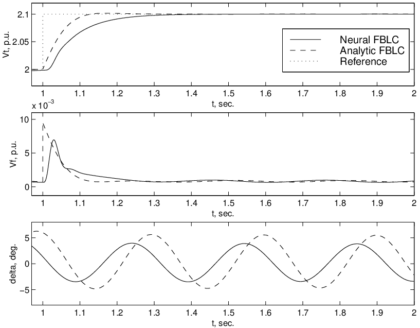
Next we test the ability of the neural and analytic excitation controllers to track reference signals at an operating point far from the nominal, i.e. from $v_{ref}=2.0$ to $v_{ref}=2.1$. The step change takes place at $t=1.0$ second and the response is depicted in Fig. 12. It is observed that similar transient response characteristics are obtained compared to the response to a perturbation about the nominal operating point as shown in Fig. 11. Also the control effort $v_{f}$ is less for the neural controller than for the analytic controller. Finally, observe that in both Fig. 11 and Fig. 12, the magnitude of the rotor angle oscillations for the neural excitation controller mimics the behaviour of the system under no control in response to a small perturbation. This is due to fact that feedback linearization was applied to a $7^{th}$ order system, as opposed to a $3^{rd}$ order, as done with analytic feedback linearization. Hence, the effect of excitation control is almost completely decoupled from the mechanical modes of the system.

Excitation controller/power system stabilizer: In [3], the control law used for the power system stabilizer is given by

$$v\;=\;-K(v_{t}-v_{ref}+K_{1}\dot{\delta}),\hskip 28.45274ptK,K_{1}>0$$

giving voltage tracking dynamics:

$$\dot{v}_{t}\;=\;-K(v_{t}-v_{ref})-KK_{1}\dot{\delta}$$

with gains

$$K\;=\;200,\hskip 28.45274ptK_{1}\;=\;0.7091$$

These values are determined by a root locus criterion (see [3]) in order to obtain optimal damping of rotor angle oscillations.

Recall that the control law for the neural adaptive controller/power system stabilizer is given by

$$u_{k}=\frac{\tilde{u}(k)-\hat{f}(\cdot)}{\hat{g}(\cdot)}+K_{pss}\cdot\dot{\delta}(k)$$

where the gain $K_{pss}$ is given by

$$K_{pss}\;=\;\nu\times 0.7091.$$

(39)

For the simulations which follow, $\nu\;=\;3.$ In general, increasing $\nu$ has the effect of improving the damping on $\delta$ for step changes in reference signal. However $\nu$ can not be assigned arbitrarily large values. For instance, values of $\nu$ much higher than $3$ have the effect of making the system unstable. The output of the system is originally at the nominal value of $v_{t}=1.1392$. A step change of $0.1p.u.$ in reference voltage occurs at $t=2.0$ seconds. Observe from Fig. 13 that the neural controller accurately tracks the reference signal (actually, tracking error is 0.0082 % after 2.8 seconds) and quickly damps out the rotor angle oscillations.

As done for the excitation controller, the controller/pss is validated for a change in operating point to $v_{ref}=2.0$ and a step change of $0.1$ p.u. takes place at $t=2.0$ seconds. Dynamic behaviour similar to that in Fig. 13 are obtained for both controllers. The figure depicting the tracking and stabilizing dynamics for this new operating point is shown in Fig. 14

The neural controller was also tested for big changes in the operating points of the system as follows: a step increase in $v_{ref}$ from $1\;p.u.$ to $2\;p.u.$ was introduced at $t=0$. After $2$ seconds, $v_{ref}$ dropped to $0.5\;p.u.$ Fig. 15 depicts the results for both the neural and analytic controllers. Both controllers performed well and exhibited similar tracking dynamics compared to the response to a small step change in reference voltage shown in Fig. 13.

The tuned analytic controller described above exhibits high frequency harmonics during tracking due to the effects of the unmodelled dynamics in the design phase. The neural model does not exhibit such pronounced oscillations. Also observe that the control effort ($v_{f}$ in Figs. 13 and 15) is several orders of magnitude higher for the analytic controller than for the neural controller. Finally, observe that the steady state tracking error is effectively zero in both cases and the speed of response is comparable.

Another set of tests done on the control system involves the inertia parameter $H$ drifting from its nominal value of $9.5$ to about $4.75$ (i.e. a $50\%$ drift) to see how well the control system behaves when feedback linearization is inexact. This is depicted in Fig. 16. The neural controller performs better than the analytic controller in this case since the analytic controller design was based on exact knowledge of all the parameters of the plant. It is observed that the tracking dynamics of the neural controller is essentially the same as what we have in Fig. 13, where the parameter $H=9.5$. For this test, the value of $\nu$ in (39) is reduced to $\nu=2.6$. For arbitrary variation in the parameters, the neural controller performance can be improved by reducing the size of the deadzone used in the adaptation algorithm so that weights are updated for values of $d_{0}$ less than $0.01$ in this particular case.

The system performance under a disturbance is investigated by forcing the mechanical power input, $P_{m}$ to drop suddenly by $33.4\%$ (from 1.6512 to 1.1); the response is shown in Fig. 17. Observe that both controllers recover quickly and restore the terminal voltage $v_{t}$ to its nominally value. The rotor angle changes to a new value but still retains its damping. In this case both controllers gave the same level of performance, although the tracking dynamics for the neural controller is just slightly better. We note that in practice this may be a rather drastic change in power level, but the simulation is done just to see how far the system may be “pushed” whilst still maintaining control action.

Finally, the effect of on-line weight adaptation on the response of the overall control system is investigated by observing the rate at which the error adaptation occurs. The Fig. 18 shows how quickly the plant output error $\{\hat{y}(k+1)-y(k+1)\}$ is adapted for the parameter variation, disturbance and normal excitation controller/power system stabilizer tests. Observe that the errors are not too large (apart from that associated with system disturbance) and are adapted quickly. Therefore it is concluded that adapting the weights online does not unduly slow down the response of the overall control system.

A neural adaptive feedback linearizing excitation controller/ power system stabilizer has been proposed for a high-order model of the synchronous machine/infinite bus power system. The controller provides tracking performance with less high frequency harmonics than an analytic controller based on a reduced-order model of the system and would seem to tolerate parameter drift. In the cases considered, step changes in reference voltage are tracked, with the neural controller requiring significantly less control effort than the analytic controller. The neural controller also provides damping of power angle oscillations with similar voltage and power angle transient characteristics over different operating points of the system. Also on-line controller adaptation does not slow down the overall control system response since output errors are reduced quickly. The advantage of this approach lies in the fact that exact knowledge of the power system dynamics is not absolutely necessary and the system state need not all be measurable. Also, the complicated mathematical mapping required to carry out analytic feedback linearization is avoided. The control scheme is quite straightforward and easy to synthesize. Thorough mathematical analyses guaranteeing convergence and/or stability for this type of control scheme (comparable to that reported in [8]) is still to be done.

References

- [1] V. S. S. Vankayala and N. D. Rao, ”Artificial neural networks and their applications to power systems - a bibliographic survey,” Electric power systems research, vol. 28, 1993, pp. 67-79
- [2] D.C. Kennedy, ”Power system excitation control and stabilization by input-output feedback linearization,” Proceedings of the 2nd Asian Control Conference, vol.3, 1997, pp. 295-298.
- [3] D. Kennedy, D. Miller and V. Quintana, ”A nonlinear geometric approach to power system excitation control and stabilization,” J. Electric Power and Energy Systems, vol. 20, issue 8, Nov. 1998, pp. 501-515.
- [4] F.K. Mak. ”Design of Nonlinear Generator Exciters Using Differential Geometric Control Theories,” Proceedings of the 31st IEEE Conference on Decision and Control, 1992, 1149-1153
- [5] D. Rumelhart, G.E. Hinton and R.J. Williams, ”Learning internal representations by error propagation,” in Parallel Distributed Processing, vol. 1, D.E. Rumelhart and J.C. McClelland, Eds. MIT Press, Cambridge, MA, 1986
- [6] J. W. Chapman, M. D. Ilić, C. A. King, L. Eng, and H. Kaufman. ”Stabilizing a multimachine power system via decentralized feedback linearizing excitation control,” IEEE Trans. Power Systems, vol. 8, 1993, pp. 830-839.
- [7] F-C Chen, ”Back-propagation neural networks for nonlinear self-tuning adaptive control,” IEEE Control Systems Magazine, Special Issue on Neural Networks for Control Systems, April 1990, pp. 44-48.
- [8] F-C Chen and H.K. Khalil, ”Adaptive control of a class of nonlinear discrete-time systems using neural networks,” IEEE Trans. Automatic Control, vol. 40, no. 5, May 1995, pp. 791-801.
- [9] A. Isidori, Nonlinear Control Systems , 2nd Edition, Springer-Verlag, New York, 1989.
- [10] D.A. Pierre, ”A perspective on Adaptive Control of Power Systems,” IEEE Trans. Power Systems, vol. 2, no. 2, 1987, pp. 386-396.
- [11] B. Jakubczyk, ”Feedback linearization of discrete time systems,” Systems and Control Letters, no. 9, 1987, pp. 411-416.
- [12] S.S. Sastry and A. Isidori, ”Adaptive control of linearizable systems,” IEEE Trans. Automatic Control, vol. 34, no. 11, Nov. 1989, pp. 1123-1131.
- [13] I. Kanellakopoulos, P.V. Kokotović, and A.S. Morse, ”Systematic design of adaptive controllers for feedback linearizable systems,” IEEE Trans. Automatic Control, vol. 36, no. 11, Nov. 1991, pp. 1241-1253.
- [14] K. Funahashi, ”On the approximate realization of continuous mappings by neural networks,” Neural Networks, vol. 2, 1989, pp. 183-192.
- [15] M. Ngaard, Neural network based system identification toolbox. Tech. Report 97-E-851, Dept. of Automation, Technical University of Denmark, 1997
- [16] P. Kundur, Power System Stability and Control, McGraw-Hill, New York, 1994.
- [17] R. Marino, ”An example of a nonlinear regulator,” IEEE Trans. Automatic Control, vol. 26, 1984, pp. 595-598.
- [18] Kingsley Fregene Neural adaptive feedback linearizing control of a high-order power system. MASc Thesis, Dept. of Electrical and Computer Engineering, University of Waterloo, Ont., Canada, 1999.