Quivers, Floer cohomology, and
braid group actions

This paper investigates the connection between symplectic geometry and those parts of representation theory which revolve around the notion of categorification. The existence of such a connection, in an abstract sense, follows from simple general ideas. The difficult thing is to make it explicit. On the symplectic side, the tools needed for a systematic study of this question are not yet fully available. Therefore we concentrate on a single example, which is just complicated enough to indicate the depth of the relationship. The results can be understood by themselves, but a glimpse of the big picture certainly helps to explain them, and that is what the present section is for.

Let $\mathcal{Q}$ be a category. An action of a group $G$ on $\mathcal{Q}$ is a family $(\mathcal{F}_{g})_{g\in G}$ of functors from $\mathcal{Q}$ to itself, such that $\mathcal{F}_{e}\cong\mathrm{id}_{\mathcal{Q}}$ and $\mathcal{F}_{g_{1}}\mathcal{F}_{g_{2}}\cong\mathcal{F}_{g_{1}g_{2}}$ for all $g_{1},g_{2}\in G$; here $\cong$ denotes isomorphism of functors¹¹ 1 Strictly speaking, this should be called a weak action of $G$ on $\mathcal{Q};$ a full-fledged action comes with preferred isomorphisms $\mathcal{F}_{g_{1}}\mathcal{F}_{g_{2}}\cong\mathcal{F}_{g_{1}g_{2}}$ that satisfy obvious compatibility relations.. We will not distinguish between two actions $(\mathcal{F}_{g})$ and $(\widetilde{\mathcal{F}}_{g})$ such that $\mathcal{F}_{g}\cong\widetilde{\mathcal{F}}_{g}$ for all $g$. A particularly nice situation is when $\mathcal{Q}$ is triangulated and the $\mathcal{F}_{g}$ are exact functors. Then the action induces a linear representation of $G$ on the Grothendieck group $K(\mathcal{Q})$. The inverse process, in which one lifts a given linear representation to a group action on a triangulated category, is called categorification (of group representations).

The connection with symplectic geometry is based on an idea of Donaldson. He proposed (in talks circa $1994$) to associate to a compact symplectic manifold $(M^{2n},\omega)$ a category $\mathrm{Lag}(M,\omega)$ whose objects are Lagrangian submanifolds $L\subset M$, and whose morphisms are the Floer cohomology groups²² 2 The definition of Floer cohomology in general involves difficult analytic and algebraic questions. To simplify the exposition, we tacitly ignore them here. $HF(L_{0},L_{1})$. The composition of morphisms would be given by products $HF(L_{1},L_{2})\times HF(L_{0},L_{1})\longrightarrow HF(L_{0},L_{2}),$ which are defined, for example, in [39]. Let $\mathrm{Symp}(M,\omega)$ be the group of symplectic automorphisms of $M$. Any $\phi\in\mathrm{Symp}(M,\omega)$ determines a family of isomorphisms $HF(L_{0},L_{1})\cong HF(\phi L_{0},\phi L_{1})$ for $L_{0},L_{1}\in\mathrm{Ob}(\mathrm{Lag}(M,\omega))$ which are compatible with the products. In other words, $\phi$ induces an equivalence $\mathcal{F}_{\phi}$ from $\mathrm{Lag}(M,\omega)$ to itself. This is just a consequence of the fact that $\mathrm{Lag}(M,\omega)$ is an object of symplectic geometry, hence natural under symplectic maps. Assume for simplicity that $H^{1}(M;\mathbb{R})=0$, so that all symplectic vector fields are Hamiltonian. Then a smooth isotopy of symplectic automorphisms $(\phi_{t})_{0\leq t\leq 1}$ gives rise to distinguished elements in $HF(\phi_{0}L,\phi_{1}L)$ for all $L.$ This means that the ${\mathcal{F}}_{\phi}$ define a canonical action of the symplectic mapping class group $\pi_{0}(\mathrm{Symp}(M,\omega))$ on $\mathrm{Lag}(M,\omega)$. As a consequence, any symplectic fibre bundle with fibre $(M,\omega)$ and base $B$ gives rise to a $\pi_{1}(B)$-action on $\mathrm{Lag}(M,\omega)$, through the monodromy map $\pi_{1}(B)\rightarrow\pi_{0}(\mathrm{Symp}(M,\omega))$. Interesting examples can be obtained from families of smooth complex projective varieties.

While it is thus easy to construct potentially interesting group actions on the categories $\mathrm{Lag}(M,\omega)$, both the group actions and the categories themselves are difficult to understand. A particularly intriguing question is whether, in any given case, one can relate them to objects defined in a purely algebraic way. In homological algebra there is a standard technique for approaching similar comparison problems (an example is Beilinson’s work [2] on coherent sheaves on $\mathbb{C}{\mathrm{P}}^{k}$). A very crude attempt to adapt this technique to our situation goes like this: pick a finite number of Lagrangian submanifolds $L_{0},\dots,L_{m}\subset M$ which, for some reason, appear to be particularly important. Using the product on Floer cohomology, turn

into a ring. Now associate to an arbitrary Lagrangian submanifold $L\subset M$ the $A$-module $\bigoplus_{i}HF(L,L_{i})$. This defines a functor from $\mathrm{Lag}(M,\omega)$ to the category of $A$-modules. As it stands the functor is not particularly useful, since it does not take into account all the available structure.

To begin with, Floer cohomology groups are graded, and hence $A$ is a graded ring (depending on $M$, this may be only a $\mathbb{Z}/N$-grading for some finite $N$). To make more substantial progress one needs to refine the category $\mathrm{Lag}(M,\omega)$. This theory is as yet under construction, and we can only give a vague outline of it. As pointed out by Fukaya [15], working directly with the Floer cochain complexes should enable one to construct an $A_{\infty}$-category underlying $\mathrm{Lag}(M,\omega)$. Kontsevich [24] suggested to consider the derived category of this $A_{\infty}$-category. This “derived Fukaya category” is expected to be triangulated, and to contain $\mathrm{Lag}(M,\omega)$ as a full subcategory; we denote it by $D^{b}\mathrm{Lag}(M,\omega)$ (which is an abuse of notation). The action of $\pi_{0}(\mathrm{Symp}(M,\omega))$ on $\mathrm{Lag}(M,\omega)$ should extend to an action on $D^{b}\mathrm{Lag}(M,\omega)$ by exact functors. Moreover, it seems natural to suppose that the Grothendieck group of $D^{b}\mathrm{Lag}(M,\omega)$ is related to $H_{n}(M;\mathbb{Z})$; that would mean that the group actions coming from families of projective varieties could be considered as categorifications of the classical monodromy representations. Returning to the rings (1.1), one expects to get from Fukaya’s construction a canonical (up to quasi-isomorphism) $A_{\infty}$-algebra ${\mathcal{A}}$ with cohomology $A$. The functor introduced above would lift to an $A_{\infty}$-functor from the $A_{\infty}$-category underlying $\mathrm{Lag}(M,\omega)$ to the $A_{\infty}$-category of $A_{\infty}$-modules over ${\mathcal{A}}$. In a second step, this would induce an exact functor

where $D({\mathcal{A}})$ is the derived category of $A_{\infty}$-modules. A standard argument based on exactness indicates that this functor, when restricted to the triangulated subcategory of $D^{b}\mathrm{Lag}(M,\omega)$ generated by $L_{0},\dots,L_{m}$, would be full and faithful. This is a much stronger comparison theorem than one could get with the primitive approach which we had mentioned first. We will not say more about this; what the reader should keep in mind is the expected importance of the rings $A$.

It should also be mentioned that there is a special reason to study actions of braid groups and mapping class groups on categories. In 1992–1994 a number of mathematicians independently suggested extending the formalism of TQFTs to manifolds with corners. While three-dimensional extended TQFTs are rather well understood, there has been much less progress in the four-dimensional case. Part of the data which make up a four-dimensional extended TQFT are categories ${\mathcal{Q}}(S)$ associated to closed surfaces $S$; these would govern the process of cutting and pasting for the vector spaces associated to closed three-manifolds. The mapping class group of $S$ should act on ${\mathcal{Q}}(S)$ in a natural way, and for interesting TQFTs this action is likely to be highly nontrivial. As a matter of historical interest, we note that the categories $\mathrm{Lag}(M,\omega)$ were invented by Donaldson in an attempt to make gauge theory fit into the extended TQFT formalism; see [16] for more recent developments.

There is a version of this for invariants of two-knots, where the categories are associated to punctured discs and carry actions of the braid groups. The papers [4] and [23] go some way towards constructing such extended TQFTs in a representation-theoretic way.

In the algebraic part of the paper, we study the derived categories $D^{b}(A_{m}\text{-}\mathrm{mod})$ for a particular family $A_{m}$ ($m\geq 1$) of graded rings. The definition of $A_{m}$ starts with the quiver (oriented graph) $\Gamma_{m}$ shown in Figure 1, whose vertices are labelled $0,1,\dots,m$. Recall that the path ring of an arbitrary quiver $\Gamma$ is the abelian group freely generated by the set of all paths in $\Gamma$, with multiplication given by composition. Paths of length $l$ in $\Gamma_{m}$ correspond to $(l+1)$-tuples $(i_{1}|i_{2}|\dots|i_{l+1})$ of numbers $i_{k}\in\{0,1,\dots,m\}$ such that the difference of any two consecutive ones is $\pm 1$. Therefore, the path ring of $\Gamma_{m}$ is the abelian group freely generated by such $(l+1)$-tuples for all $l\geq 0$, with the multiplication

The paths $(i)$ of length zero are mutually orthogonal idempotents, and their sum is the unit element. We make the path ring of $\Gamma_{m}$ into a graded ring by setting $\deg(i)=\deg(i|i+1)=0$ and $\deg(i+1|i)=1$ for all $i$, and extending this in the obvious way (this is not the same as the grading by lengths of paths). Finally, $A_{m}$ is the quotient of the path ring of $\Gamma_{m}$ by the relations

for all $0<i<m$. These relations are homogeneous with respect to the above grading, so that $A_{m}$ is a graded ring. As an abelian group $A_{m}$ is free and of finite rank; a basis is given by the $4m+1$ elements $(0),\dots,(m),(0|1),\dots(m-1|m),(1|0),\dots,(m|m-1),(1|0|1),\dots,(m|m-1|m)$.

Let $A_{m}\text{-}\mathrm{mod}$ be the category of finitely generated graded left $A_{m}$-modules, and $D^{b}(A_{m}\text{-}\mathrm{mod})$ its bounded derived category. We will write down explicitly exact self-equivalences ${\mathcal{R}}_{1},\dots,{\mathcal{R}}_{m}$ of $D^{b}(A_{m}\text{-}\mathrm{mod})$ which satisfy

These are the defining relations of the braid group $B_{m+1}$, which means that the functors $\mathcal{R}_{i}$ generate an action $(\mathcal{R}_{\sigma})_{\sigma\in B_{m+1}}$ of $B_{m+1}$ on $D^{b}(A_{m}\text{-}\mathrm{mod})$. The first step in analyzing this action is to look at the induced linear representation on the Grothendieck group $K(D^{b}(A_{m}\text{-}\mathrm{mod}))\cong K(A_{m}\text{-}\mathrm{mod})$. The category $A_{m}\text{-}\mathrm{mod}$ carries a self-equivalence $\{1\}$ which raises the grading of a module by one (this should not be confused with the translation functor $[1]$ in the derived category). The action of $\{1\}$ makes $K(A_{m}\text{-}\mathrm{mod})$ into a module over $\mathbb{Z}[q,q^{-1}]$. In fact

a basis is given by the indecomposable projective modules $P_{i}=A_{m}(i)\subset A_{m}$. The functors ${\mathcal{R}}_{i}$ commute with $\{1\}.$ Therefore the induced representation is a homomorphism $B_{m+1}\longrightarrow GL_{m+1}(\mathbb{Z}[q,q^{-1}])$. A computation shows that this is the well-known Burau representation.

At this point, it is helpful to recall the topological meaning of the Burau representation. Take a closed disc $D$ and a set $\Delta\subset D\setminus\partial D$ of $(m+1)$ marked points on it. Let $\widetilde{D}$ be the infinite cyclic cover of $D\setminus\Delta$ whose restriction to a small positively oriented loop around any point of $\Delta$ is isomorphic to $\mathbb{R}\longrightarrow S^{1}$. Fix a point $z$ on $\partial D$, and let $\tilde{z}\subset\widetilde{D}$ be its preimage. Let $\mathcal{G}=\mathrm{Diff}(D,\partial D;\Delta)$ be the group of diffeomorphisms $f$ of $D$ which satisfy $f|\partial D=\mathrm{id}$ and $f(\Delta)=\Delta$. Any $f\in\mathcal{G}$ can be lifted in a unique way to a $\mathbb{Z}$-equivariant diffeomorphism of $\widetilde{D}$ which acts trivially on $\tilde{z}$. The Burau representation can be defined as the induced action of $\pi_{0}(\mathcal{G})\cong B_{m+1}$ on $H_{1}(\widetilde{D},\tilde{z};\mathbb{Z})\cong\mathbb{Z}[q,q^{-1}]\otimes\mathbb{Z}^{m+1}$. Our first result will show that the action $(\mathcal{R}_{\sigma})$ itself, or rather certain numbers attached to it, admits a similar topological interpretation. For any $\sigma\in B_{m+1}$ and $0\leq i,j\leq m$ consider the bigraded abelian group

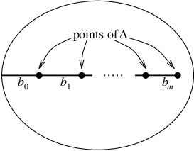
Fix a collection of curves $b_{0},\dots,b_{m}$ on $(D,\Delta)$ as in Figure 2; this determines a preferred isomorphism $\pi_{0}(\mathcal{G})\cong B_{m+1}$. Take some $\sigma\in B_{m+1}$ and a diffeomorphism $f_{\sigma}\in\mathcal{G}$ representing it. The geometric intersection number $I(b_{i},f_{\sigma}(b_{j}))\geq 0$ counts the number of essential intersection points between the curves $b_{i}$ and $f_{\sigma}(b_{j})$. The exact definition, which is a slight variation of the usual one, will be given in the body of the paper.

We will actually prove a slightly stronger result, which describes (1.2) up to isomorphism in terms of bigraded intersection numbers invented for that purpose. Theorem 1.1, together with standard properties of geometric intersection numbers, has an interesting implication. Call a group action $(\mathcal{F}_{g})_{g\in G}$ on a category $\mathcal{Q}$ faithful if $\mathcal{F}_{g}\not\cong\mathrm{id}_{\mathcal{Q}}$ for all $g\neq e$.

Note that this cannot be proved by considerations on the level of Grothendieck groups, since the Burau representation is not faithful (in the usual sense of the word) for $m\gg 0$ [27]. Corollary 1.2 can be used to derive the faithfulness of certain braid group actions on categories which occur in algebraic geometry [38].

On the symplectic side we will study the Milnor fibres of certain singularities. The $n$-dimensional singularity of type $(A_{m})$, for $m,n\geq 1$, is the singular point $x=0$ of the hypersurface $\{x_{0}^{2}+\dots+x_{n-1}^{2}+x_{n}^{m+1}=0\}$ in $\mathbb{C}^{n+1}$. To define the Milnor fibre one perturbs the defining equation, so as to smooth out the singular point, and then intersects the outcome with a ball around the origin. In the present case one can take

where $h(z)=z^{m+1}+w_{m}z^{m}+\dots+w_{1}z+w_{0}\in\mathbb{C}[z]$ is a polynomial with no multiple zeros, with $w=(w_{0},\dots,w_{m})\in\mathbb{C}^{m+1}$ small. Equip $M$ with the restriction $\omega$ of the standard symplectic form on $\mathbb{C}^{n+1}$, and its boundary with the restriction $\alpha$ of the standard contact one-form on $S^{2n+1}$. Assume that the disc $D$ considered above is in fact embedded in $\mathbb{C}$ as the subset $\{z\in\mathbb{C},\;|z|^{2}+|h(z)|\leq 1\}$, and that the set of marked points is $\Delta=h^{-1}(0)$. Then one can associate to any curve $c$ in $(D,\Delta)$ a Lagrangian submanifold $L_{c}$ of $(M,\omega,\alpha)$. We postpone the precise definition, and just mention that $L_{c}$ lies over $c$ with respect to the projection to the $x_{n}$-variable. In particular, from curves $b_{0},\dots,b_{m}$ as in Figure 2 one obtains Lagrangian submanifolds $L_{0},\dots,L_{m}$. These are all $n$-spheres except for $L_{0}$, which is an $n$-ball with boundary in $\partial M$; they intersect each other transversally, and

The case $m=3$ and $n=1$ is shown in Figure 3.

By varying the polynomial $h$ one gets a family of Milnor fibres parametrized by an open subset $W\subset\mathbb{C}^{m+1}$. Parallel transport in this family, for a suitable class of connections, defines a symplectic monodromy map

The actual construction is slightly more complicated than this rough description may suggest. Similar maps can be defined for general hypersurface singularities. In our particular case, there are isomorphisms

the first one comes from a canonical embedding $W\subset\mathrm{Conf}_{m+1}(D\setminus\partial D)$, the second one is well-known and again canonical, and the third one is determined by the choice of curves $b_{0},\dots,b_{m}$ as before. Using these isomorphisms, one can consider $\rho_{s}$ as a homomorphism from the braid group to $\pi_{0}(\mathrm{Symp}(M,\partial M,\omega))$. We mention, although this has no relevance for the present paper, that there is a more direct definition of $\rho_{s}$ in terms of generalized Dehn twists along $L_{1},\dots,L_{m}$. This is explained in [37, Appendix] for $n=2$, and the general case is similar.

Take some $\sigma\in B_{m+1}$ and a map $\phi_{\sigma}\in\mathrm{Symp}(M,\partial M,\omega)$ which represents $\rho_{s}(\sigma)$ in the sense of (1.4). If $n=1$ we also assume that $\phi_{\sigma}$ has a particular property called $\theta$-exactness, which will be defined in the body of the paper; this assumption is necessary because in that dimension $H^{1}(M,\partial M;\mathbb{R})\neq 0$. The Floer cohomology $HF(L_{i},\phi_{\sigma}(L_{j}))$ is a finite-dimensional vector space over $\mathbb{Z}/2$ constructed from the intersection points of $L_{i}$ and $\phi_{\sigma}(L_{j})$, and it is independent of the choice of $\phi_{\sigma}$.

Here $f_{\sigma}\in\mathrm{Diff}(D,\partial D;\Delta)$ is as in Theorem 1.1. There is also a faithfulness result analogous to Corollary 1.2:

It is instructive to compare this with the outcome of a purely topological consideration. The classical geometric monodromy $\rho_{g}$ is the composition

where the vertical arrow is induced by inclusion. For $n=1$ this arrow is an isomorphism, and the injectivity of $\rho_{g}$ is an old result of Birman and Hilden [7] (see Proposition 3.11). The situation changes drastically for $n=2$, where Brieskorn’s simultaneous resolution [8] implies that $\rho_{g}$ factors through the symmetric group $S_{m+1}$. The difference between $\rho_{s}$ and $\rho_{g}$ in this case shows that the symplectic structure of the Milnor fibre contains essential information about the singularity, which is lost when one considers it only as a smooth manifold. The situation for $n\geq 3$ is less clear-cut. One can use unknottedness results of Haefliger [19], together with an easy homotopy computation, to show that $\rho_{g}$ is not injective for all $m\geq 2$ if $n>2$ is even, and for all $m\geq 3$ if $n\equiv 1\,\text{mod}\,4$, $n\neq 1$ (with more care, these bounds could probably be improved).

By combining Theorems 1.1 and 1.3 one sees that the dimension of $HF(L_{i},\phi_{\sigma}(L_{j}))$ is equal to the total rank of (1.2). One can refine the comparison by taking into account the graded structure of Floer cohomology, as follows:

Strictly speaking, the grading in Floer theory is canonical only up to an overall shift (in fact, for $n=1$ there is an even bigger ambiguity), and the isomorphism holds for a particular choice. One can cure this problem by using Kontsevich’s idea of graded Lagrangian submanifolds. We will not state the corresponding improved version of Corollary 1.5 explicitly, but it can easily be extracted from our proof. Note that if one looks at the graded groups $HF^{*}(L_{i},\phi_{\sigma}(L_{j}))$ in isolation, they appear to depend on $n$ in a complicated way; whereas the connection with the bigraded group (1.2) makes this dependence quite transparent.

One can see this collapsing of the bigrading on a much simpler level, which corresponds to passing to Euler characteristics on both sides in Corollary 1.5. Namely, the representation of the braid group on $H_{n}(M,\partial L_{0};\mathbb{Z})\cong\mathbb{Z}^{m+1}$ induced by $\rho_{s}$ is the specialization $q=(-1)^{n}$ of the Burau representation.

While our proof of Corollary 1.5 is by dimension counting, it is natural to ask whether there are canonical homomorphisms between the two graded groups; these should be compatible with the product structures existing on both sides. Unfortunately, the techniques used here are not really suitable for that; while an inspection of our argument suggests a possible definition of a homomorphism in (1.5), showing that it is independent of the various choices involved would be extremely complicated. And there is no easy way to adapt the proof of Theorem 1.3 to include a description of the product on Floer cohomology. It seems that to overcome these problems, one would have to use a more abstract approach, in line with the general picture of Section 1a. While the details of this are far from clear, an outline can easily be provided, and we will do that now.

It is convenient to modify the algebraic setup slightly. Let $A_{m,n}$ be the graded algebra obtained from $A_{m}$ by multiplying the grading with $n$ and changing the coefficients to $\mathbb{Z}/2$; regard this as a differential graded algebra $\widehat{A}_{m,n}$ with zero differential, and take the derived category of differential graded modules $D(\widehat{A}_{m,n})$. From the way in which $L_{0},\dots,L_{m}\subset M$ intersect each other, and standard properties of Floer cohomology, one can see that

(actually, this was the starting point of our work). It seems reasonable to assume that the $A_{\infty}$-algebra of Floer cochain complexes underlying the right hand side should be formal (see [38] for much more about this), which would make its derived category of $A_{\infty}$-modules equivalent to $D(\widehat{A}_{m,n})$. As mentioned in Section 1a, the general features of the construction should imply that one has an exact functor $D^{b}\mathrm{Lag}(M,\omega)\rightarrow D(\widehat{A}_{m,n})$, which would be full and faithful on the triangulated subcategory of $D^{b}\mathrm{Lag}(M,\omega)$ generated by $L_{0},\dots,L_{m}$. $\rho_{s}$ defines a braid group action on $\mathrm{Lag}(M,\omega)$, and there should be an induced action on $D^{b}\mathrm{Lag}(M,\omega)$. On the other hand, one can define a braid group action on $D(\widehat{A}_{m,n})$ in a purely algebraic way, in the same way as we have done for the closely related category $D^{b}(A_{m}\text{-}\mathrm{mod})$. It is natural to conjecture that the exact functor should intertwine the two actions. This would imply Corollary 1.5, in a stronger form which repairs the deficiencies mentioned above.

Finally, the reader may be wondering whether the objects which we have considered can be used to define invariants of two-knots. The category $D^{b}(A_{m}\text{-}\mathrm{mod})$ is certainly not rich enough for this. However, it has been conjectured [4] that one can construct invariants of two-knots from a certain family of categories, of which $D^{b}(A_{m}\text{-}\mathrm{mod})$ is the simplest nontrivial example. The homology groups for classical knots introduced in [23] are part of this program.

Note. During the final stage of work on this paper we learned of a preprint [33] by Rouquier and Zimmermann. They construct a braid group action in the derived category of modules over multiplicity one Brauer tree algebras, which are close relatives of $A_{m}$ (the idempotent $(0)$ of $A_{m}$ is set to zero; these smaller algebras also appear in [38] and [21]). Our action essentially coincides with the one of Rouquier and Zimmermann.

Acknowledgements. M.K. would like to thank Maxim Vybornov who introduced him to the algebras $A_{m}$ by pointing out that they describe perverse sheaves on projective spaces. The construction of the Lagrangian submanifolds $L_{c}$ was suggested to P.S. by Simon Donaldson. Most of this work was done at the Institute for Advanced Study, during the year 97/98 and two shorter visits later on. We are very grateful to the Institute, and to Robert MacPherson in particular, for making this collaboration possible. M.K. was supported by NSF grants DMS 96-27351 and DMS 97-29992 and, later on, by the University of California at Davis. P.S. was supported by NSF grant DMS-9304580 and by the Institut Universitaire de France.

Fix $m\geq 1$. We recall some of the objects introduced in Section 1b:

• •

  the graded ring $A_{m}$. In future all left modules, right modules, or bimodules over $A_{m}$ are understood to be graded;

• •

  the category $A_{m}\text{-}\mathrm{mod}$, whose objects are finitely generated $A_{m}$-modules, and whose morphisms are grading-preserving module homomorphisms. In future, we call the objects of $A_{m}\text{-}\mathrm{mod}$ just $A_{m}$-modules, and write $\mathrm{Hom}(M,N)$ instead of $\mathrm{Hom}_{A_{m}\text{-}\mathrm{mod}}(M,N)$; Throughout the paper, all homomorphisms are assumed grading-preserving unless otherwise mentioned.

• •

  the self-equivalence $\{1\}$ of $A_{m}\text{-}\mathrm{mod}$ which shifts the grading upwards by one;

• •

  the $A_{m}$-modules $P_{i}=A_{m}(i).$ These are indecomposable and projective. In fact, if one considers $A_{m}$ as a left module over itself, it splits into the direct sum $\bigoplus_{i=0}^{m}P_{i}$. Conversely, any indecomposable projective $A_{m}$-module is isomorphic to $P_{i}\{k\}$ for some $i$ and $k$.

Similarly, if one considers $A_{m}$ as a right module over itself, it splits into the direct sum of the indecomposable projective right modules ${}_{i}P=(i)A_{m}$.

For $1\leq i\leq m$ let $P_{i}\otimes\hskip 2.168pt{}_{i}P$ be the $A_{m}$-bimodule obtained by tensoring $P_{i}$ and ${}_{i}P$ over $\mathbb{Z}.$ Let $\mathcal{U}_{i}:A_{m}\mathrm{-mod}\to A_{m}\mathrm{-mod}$ be the functor of tensoring with this bimodule,

This functor is exact (since $P_{i}\otimes\hskip 2.168pt_{i}P$ is right projective) and takes projective modules to projective modules³³ 3 $i=0$ case is excluded, for although $\mathcal{U}_{0}$ can be defined, it does not satisfy the isomorphisms in Theorem 2.2..

For an abelian category $\mathcal{Q}$ denote by $P(\mathcal{Q})$ the homotopy category of bounded complexes of projective objects in $\mathcal{Q}.$ An object $M$ of $P(\mathcal{Q})$ is a bounded complex of projective objects:

A morphism $f$ from $M$ to $N$ is a collection of maps $f^{i}:M^{i}\to N^{i}$ that intertwine differentials in $M$ and $N,$ $f^{i+1}\partial_{M}^{i}=\partial_{N}^{i}f^{i}$ for all $i.$ Two morphisms $f,g$ are equal (homotopic) if there are maps $h^{i}\in\mathrm{Hom}_{\mathcal{Q}}(M^{i},N^{i-1})$ such that $f^{i}-g^{i}=h^{i+1}\partial_{M}^{i}+\partial_{N}^{i-1}h^{i}$ for all $i.$

As usual, $[k]$ denotes the self-equivalence of $P({\mathcal{Q}})$ which shifts a complex $k$ degrees to the left: $M[k]^{i}=M^{k+i},\hskip 2.168pt\partial_{M[k]}=(-1)^{k}\partial_{M}.$ Given a map of complexes $f:M\to N,$ the cone of $f$ is the complex $C(f)=M[1]\oplus N$ with the differential $\partial_{C(f)}(x,y)=(-\partial_{M}x,f(x)+\partial_{N}y).$ We refer the reader to [17] for more information about homotopy and derived categories.

If $\mathcal{Q}$ has finite homological dimension, then $P(\mathcal{Q})$ is equivalent to the bounded derived category $D^{b}(\mathcal{Q})$ of $\mathcal{Q}.$ This applies to ${\mathcal{Q}}=A_{m}\text{-}\mathrm{mod}$ by Proposition 2.1. We will use $P(A_{m}\text{-}\mathrm{mod})$ instead of $D^{b}(A_{m}\text{-}\mathrm{mod})$ throughout, and denote it by ${\mathcal{C}}_{m}=P(A_{m}\text{-}\mathrm{mod}).$

The shift automorphism $\{k\}$ of $A_{m}\text{-}\mathrm{mod}$ extends in the obvious way to an automorphism of ${\mathcal{C}}_{m}$ which we also denote by $\{k\}$. Note that $\{k\}$ and $[k]$ are quite different. In fact, if we forget about the module structure and differential, objects of ${\mathcal{C}}_{m}$ are bigraded abelian groups, so that it is natural to have two shift-like functors. Correspondingly, for any two such objects $M,N$ there is a bigraded morphism group (of finite total rank)

Let $R=(R^{j},\partial^{j})$ be a bounded complex of $A_{m}$-bimodules which are left and right projective, i.e. each $R^{j}$ is a projective left $A_{m}$-module and a projective right $A_{m}$-module. One associates to $R$ the functor ${\mathcal{R}}:{\mathcal{C}}_{m}\to{\mathcal{C}}_{m}$ of tensoring with $R:$

Define homomorphisms $\beta_{i},\gamma_{i},1\leq i\leq m,$ of $A_{m}$-bimodules

by

(when $i=m$ we omit the term $(i+1|i)\otimes(i|i+1)$ from the sum for $\gamma_{i}(1).$)

These homomorphisms induce natural transformations, also denoted $\beta_{i},\gamma_{i},$ between the functor $\mathcal{U}_{i}$, suitably shifted, and the identity functor:

Let ${R}_{i}$ be the complex of bimodules

with $A_{m}$ in degree $0.$ Denote by ${R}^{\prime}_{i}$ the complex of bimodules

with $A_{m}$ in degree $0.$ Next, we introduce functors ${\mathcal{R}}_{i}$ and ${\mathcal{R}}_{i}^{\prime}$ of tensoring with the complexes ${R}_{i}$ and ${R}^{\prime}_{i}$ respectively:

The functor ${\mathcal{R}}_{i}$ can be viewed as the cone of $\beta_{i},$ and ${\mathcal{R}}_{i}^{\prime}$ as the cone of $-\gamma_{i},$ shifted by $[-1].$

References

- [1] V. I. Arnol’d, Some remarks on symplectic monodromy of Milnor fibrations, The Floer Memorial Volume (H. Hofer, C. Taubes, A. Weinstein, and E. Zehnder, eds.), Progress in Mathematics, vol. 133, Birkhäuser, 1995, pp. 99–104.
- [2] A. A. Beilinson, Coherent sheaves on and problems of linear algebra, Funct. Anal. Appl. 12 (1978), 214–216.
- [3] A. Beilinson, V.Ginzburg and W.Soergel, Koszul duality patterns in representation theory, Journal of the AMS 9, n.2, (1996), 473–527.
- [4] J. Bernstein, I. Frenkel, and M. Khovanov, A categorification of the Temperley-Lieb algebra and Schur quotients of via projective and Zuckerman functors, Selecta Math., New ser. 5, (1999), 199–241; math.QA/0002087.
- [5] J. Bernstein and S. Gelfand, Tensor products of finite and infinite dimensional representations of semisimple Lie algebras, Compositio Math. 41, (1980), 245–285.
- [6] J. Birman, Braids, links and mapping class groups, Annals of Math. Studies 82, Princeton University Press, 1974.
- [7] J. S. Birman and H. M. Hilden, On isotopies of homeomorphisms of Riemann surfaces, Annals of Math. 97 (1973), 424–439.
- [8] E. Brieskorn, Über die Auflösung gewisser Singularitäten von holomorphen Abbildungen, Math. Ann. 166 (1966), 76–102.
- [9] Ya. Eliashberg, H. Hofer, and D. Salamon, Lagrangian intersections in contact geometry, Geom. Funct. Anal. 5 (1995), 244–269.
- [10] A. Fathi, F. Laudenbach, and V. Poénaru, Travaux de Thurston sur les surfaces, Astérisque, vol. 66–67, Soc. Math. France, 1979.
- [11] A. Floer, Morse theory for Lagrangian intersections, J. Differential Geom. 28 (1988), 513–547.
- [12] by same author, A relative Morse index for the symplectic action, Comm. Pure Appl. Math. 41 (1988), 393–407.
- [13] by same author, Witten’s complex and infinite dimensional Morse theory, J. Differential Geom. 30 (1989), 207–221.
- [14] A. Floer, H. Hofer, and D. Salamon, Transversality in elliptic Morse theory for the symplectic action, Duke Math. J. 80 (1995), 251–292.
- [15] K. Fukaya, Morse homotopy, -categories, and Floer homologies, Proceedings of GARC workshop on Geometry and Topology (H. J. Kim, ed.), Seoul National University, 1993.
- [16] by same author, Floer homology for three-manifolds with boundary I, Preprint, 1997.
- [17] S. Gelfand, Yu. Manin, Methods of homological algebra, Springer-Verlag, Berlin, 1996.
- [18] F. M. Goodman and H. Wenzl, The Temperley-Lieb algebra at roots of unity, Pacific J. Math. 161, (1993), no.2, 307–334.
- [19] A. Haefliger, Plongements différentiables des variétés dans variétés, Comm. Math. Helv. 36 (1962), 47–82.
- [20] H. Hofer, Pseudoholomorphic curves in symplectizations with applications to the Weinstein conjecture in dimension three, Invent. Math. 114 (1993), 515–563.
- [21] S. Huerfano and M. Khovanov, A category for the adjoint representation, math.QA/0002087.
- [22] R. S. Irving, Projective modules in the category , preprint, 1982.
- [23] M. Khovanov, A categorification of the Jones polynomial, Duke Math. J. 101, (2000), no.3, 359–426; math.QA/9908171.
- [24] M. Kontsevich, Homological algebra of mirror symmetry, Proceedings of the International Congress of Mathematicians (Zürich, 1994), Birkhäuser, 1995, pp. 120–139.
- [25] P. Martin, Potts models and related problems in statistical mechanics, Series on Advances in Statistical Mechanics, vol.5, 1991, World Scientific.
- [26] D. McDuff and D. Salamon, Introduction to Symplectic Topology, Oxford University Press, 1995.
- [27] J. Moody, The Burau representation of the braid group is unfaithful for large , Bull. Amer. Math. Soc. 25 (1991), 379–384.
- [28] Y.-G. Oh, Floer cohomology of Lagrangian intersections and pseudo-holomorphic discs I, Comm. Pure Appl. Math. 46 (1993), 949–994.
- [29] by same author, On the structure of pseudo-holomorphic discs with totally real boundary conditions, J. Geom. Anal. 7 (1997), 305–327.
- [30] by same author, Floer theory for non-compact Lagrangian submanifolds, Preprint, 2000.
- [31] M. Poźniak, Floer homology, Novikov rings and clean intersections, Northern California Symplectic Geometry Seminar, 119–181, AMS Transl. Ser. 2, 196, AMS, Providence, RI, 1999.
- [32] J. Robbin and D. Salamon, The Maslov index for paths, Topology 32 (1993), 827–844.
- [33] R. Rouquier and A. Zimmermann, Picard groups for derived module categories, preprint, 1998, http://www.math.jussieu.fr/rouquier/.
- [34] D. Salamon, Morse theory, the Conley index, and Floer homology, Bull. London Math. Soc. 22 (1990), 113–140.
- [35] D. Salamon and E. Zehnder, Morse theory for periodic solutions of Hamiltonian systems and the Maslov index, Comm. Pure Appl. Math. 45 (1992), 1303–1360.
- [36] P. Seidel, Graded Lagrangian submanifolds, Bull. Soc. Math. France 128 (2000), 103-149; math.SG/9903049.
- [37] by same author, Lagrangian two-spheres can be symplectically knotted, J. Differential Geom. 52 (1999), 147–173; math.DG/9803083.
- [38] P. Seidel and R. Thomas, Braid group actions on derived categories of coherent sheaves, math.AG/0001043.
- [39] V. De Silva, Products in the symplectic Floer homology of Lagrangian intersections, Ph.D. thesis, Oxford University, 1998.
- [40] C. Viterbo, Intersection des sous-variétés Lagrangiennes, fonctionelles d’action et indice des systèmes Hamiltoniens, Bull. Soc. Math. France 115 (1987), 361–390.
- [41] A. Weinstein, Lagrangian submanifolds and hamiltonian systems, Annals of Math. 98 (1973), 377–410.
- [42] B.W.Westbury, The representation theory of the Temperley-Lieb algebras, Math. Z. 219, (1995) no.4, 539-565.