Calculus of clovers and finite type invariantsof 3–manifolds
Abstract
A clover is a framed trivalent graph with some additional structure, embedded in a 3–manifold. We define surgery on clovers, generalizing surgery on Y–graphs used earlier by the second author to define a new theory of finite-type invariants of 3–manifolds. We give a systematic exposition of a topological calculus of clovers and use it to deduce some important results about the corresponding theory of finite type invariants. In particular, we give a description of the weight systems in terms of uni-trivalent graphs modulo the AS and IHX relations, reminiscent of the similar results for links. We then compare several definitions of finite type invariants of homology spheres (based on surgery on Y–graphs, blinks, algebraically split links, and boundary links) and prove in a self-contained way their equivalence.
keywords
3–manifolds, Y–graphs, finite type invariants, cloverspolyak@math.tau.ac.il
57N10, 57M27 \secondaryclass57M25
eometry & opology Volume 5 (2001) 75–108\nlPublished: 10 February 2001
Email:\stdspace\theemail
URL:\stdspace\theurl
Abstract
AMS Classification numbers Primary: \theprimaryclass
Secondary: \thesecondaryclass
Keywords \thekeywords
Proposed: Robion Kirby Received: 19 October 2000\nlSeconded: Joan Birman, Cameron Gordon Accepted: 28 January 2001
1 Introduction
1.1 Finite type invariants
Polynomials play a fundamental role in mathematics. Here is one of the possible definitions of a polynomial using a discrete version of the -th derivative. Let be a vector space over a field . For and , denote and . A function is a polynomial of degree less than , iff for any . This definition has a significant advantage over the standard definition of a polynomial, since it can be easily considered in a more general setup. In particular, and may be just abelian groups.
Finite type invariants play the role of polynomial functions in topology. In this setting, however, the situation is somewhat more tricky, and involves a choice of an appropriate analog of both the zero element and the addition operation in . In the last decade, this general idea was successfully used in knot theory under the name of Vassiliev invariants. This paper is devoted exclusively to a study of a theory of finite type invariants of 3–manifolds, initiated by the second author.
The present paper was started in September 1998 in an attempt to present unpublished results by the second author. In June 1999, when this paper was still in its initial stage, the second author passed away in a tragic accident. As a result, many details and proofs were lost. We tried our best to reconstruct them and to present our results in his style and spirit.
The authors were partially supported by BSF grant 97-00398 and by NSF grant DMS-98-00703.
1.2 Finite type invariants of 3–manifolds
Several authors developed different theories of finite type invariants of integer homology spheres. All these approaches are based on the cut-and-paste technique along different types of handlebodies. Historically the first, the theory of T Ohtsuki [Oh] is based on surgery on algebraically split links and is by now relatively well understood. The first author [Ga] proposed then a theory based on surgery on boundary links, which remained relatively undeveloped. Subsequently, the first author and J Levine [GL] considered theories based on surgery on blinks, and on gluings along surfaces using elements of the Torelli group. All these theories turn out to be equivalent (up to a 2–torsion), see Section 1.8.
The second author initiated in [Gu2] a new theory of finite type invariants for arbitrary 3–manifolds, based on surgery along Y–graphs (see [Gu1, Gu2]). The latter theory has some important advantages. Firstly, it allows a unified treatment of links, graphs and 3–manifolds (possibly with boundary or a Spin–structure). It is by now relatively well understood for rational homology spheres. Secondly, other theories mentioned above have a technical drawback: the corresponding classes of surgery links are not preserved under handle slides. Finally, this theory comes equipped with a powerful topological calculus (introduced in [Gu1]), that is well-suited for a study of 3–manifolds and for explicit computations. This calculus is similar to Kirby’s calculus of framed links, but instead of cutting, twisting and regluing solid tori, in the clover calculus one performs similar operations with solid handlebodies of higher genus. The role of framed links is played here by clovers, which are framed trivalent graphs with some additional structure.
The main goals of the paper are:
- •
- •
To show, as an application, in an elementary and self-contained way, that all the above mentioned theories of finite type invariants of integer homology spheres, properly indexed, coincide over (see Section 1.8).
Independently and being uninformed about the results of the second author, K Habiro developed a theory of claspers [Ha] and used it to study finite type invariants of links. He also announced in [Ha, Section 8.4] that his theory can be extended to the study of finite type invariants of 3–manifolds and gave a brief outline of this extension. It is based on allowable graph claspers, which differ from the type of claspers considered in the rest of Habiro’s paper. In particular, the basic claspers, which were Habiro’s main tool in the theory for links, are not allowed in this setting. In general it is plausible that invariants of links can be extended to invariants of 3–manifolds. In the case in hand, however, this extension is rather nontrivial and involves new ideas presented here.
The initial data, the way to describe the basic objects, and the graphical calculus in the clasper and clover theories are somewhat different. However, while different in some aspects, these two theories essentially coincide, with surgery on allowable graph claspers being equivalent to surgery on clovers. This independent discovery of almost the same theory by two non-interacting researchers looks rather promising, ruling out an element of arbitrariness. Some results announced by K Habiro [Ha, Section 8.4] seem to overlap with those discussed in Sections 2–4 below. Unfortunately, it seems that presently there is no available manuscript with the exact statements and proofs of Habiro’s results for 3–manifolds. We apologize in advance for any possible overlaps. It should be also mentioned that T Cochran and P Melvin [CM] proposed an extension of Ohtsuki’s theory to arbitrary 3–manifolds. Their theory, unlike the one considered in this paper, preserves triple cup-products, and the relation between these theories is more complicated.
1.3 Y–graphs
Throughout this paper by a manifold we mean a smooth oriented compact connected 3–manifold.
We recall some definitions from [Gu2]. The graph shown in Figure 1a is called a standard Y–graph. The edges of are framed with a vector field normal to the plane of the picture. A framed graph in a 3–manifold is called a Y–graph, if it is the image of under a smooth embedding of a neighborhood of . The embedding can be recovered from up to isotopy. Let be the six component link in shown in Figure 1b. All components of are 0–framed. Surgery on along the framed link is called a surgery along , or a Y–surgery. A Y–surgery can be realized by cutting a solid genus 3 handlebody and regluing it in another way (see [Ma]). The resulting manifold is defined up to a diffeomorphism, which is the identity outside of a small neighborhood of the Y–graph. Denote it by .

An equivalent surgery, under the name of Borromean surgery was considered by S Matveev. As shown in [Ma], two manifolds can be connected by a sequence of Borromean surgeries, if and only if they have the same homology and the linking pairing in . In particular, can be obtained from by Y–surgeries, iff is an integer homology sphere (HS in short).
A Y–link in a manifold is a collection of disjoint Y–graphs in . By surgery on we mean surgery on each Y–graph in . Pushing out the Y–graphs of the following surgeries from the previously reglued handlebodies, we can present a sequence of Y–surgeries by surgery on a Y–link.
1.4 Colored Y–links and the filtration
An –coloring of a Y–link is its splitting into disjoint subcollections , ,…, of Y–graphs. The coloring is simple, if each subcollection consists of a single Y–graph.
For an –tuple , let be the number of ones in and put . In an abelian group generated by all 3–manifolds, put
for a colored Y–link in .
Let be the subgroup of , generated by for all Y–links , colored in at least colors. This defines a decreasing filtration .
Given a Y–link in without a specified coloring, by we mean the above alternating sum for a simple coloring of .
Lemma 1.1.
The subgroup is generated by for all simply colored Y–links with at least components.
Proof.
Let be an –colored Y–link with components. We call the defect of the coloring. If , the coloring is simple. Suppose ; then there are at least two components of the same color . Therefore, the –colored Y–sublink of can be split into two disjoint non-empty parts and . It is easy to see that
where is obtained from by recoloring all components of in a new, -th, color. The defect of the coloring for each of , and is less than . The statement follows by the induction on . ∎
Thus, without a loss of generality, one can assume that the colorings in the definition of are simple.
1.5 The filtration
Further on we will be mainly interested in being a HS. Denote by .
Lemma 1.2.
Let be an –colored Y–link in a HS . Then .
Proof.
It suffices to prove, that there exist two Y–links and in , each colored in at least colors, such that .
Since is a HS, it may be obtained from by Y–surgery on a Y–link in . Let be an –colored Y–link in , such that its image under Y–surgery on is isotopic to . Let be the –colored Y–link, obtained from by an addition of , with all components of colored in a new color. Then and hence . ∎
1.6 The filtrations and
A link in a HS is algebraically split if all pairwise linking numbers of its components vanish. Such a link is boundary if all its components bound non-intersecting surfaces. A framing of is unimodular if the self-linking of each component is . Surgery on (any sublink of) a unimodular algebraically split link gives again a HS. Using these classes of links, T Ohtsuki [Oh] and the first author [Ga] introduced two different filtrations on a vector space generated by all HS. Below we describe the corresponding filtrations on the free abelian group generated by all HS.
For a framed link in , denote by the result of surgery of along . In , let
where is the number of components of a sublink . Let (respectively ) be the subgroup of , generated by for all algebraically split (respectively boundary) unimodular links in HS with at least components. As shown in [Oh] and [Ga], in the definitions of these filtrations it suffices to consider only .
1.7 The filtration
In [GL], J Levine and the first author considered another filtration, based on a notion of a blink. A blink is a framed link with a given splitting of the set of its components into pairs , such that:
- •
each pair bounds an orientable surface , so that for ;
- •
the surface induces a preferred framing of and ; this framing should differ by from the given framing of .
A sub-blink of is obtained from by a removal of some pairs . In , put
where is the number of pairs in a sub-blink . Let be the subgroup of , generated by for all blinks in a manifold with at least pairs of components.
In the same paper [GL] several other filtrations were introduced, using different subgroups of the mapping class group. Each of them was shown to be equivalent to one of the above filtrations.
1.8 The main results
We describe a topological calculus of surgery on Y–links, developed by the second author. Using this calculus, we describe the structure of the graded groups , where is the group of binary rational numbers.
We also compare different filtrations:
- •
;
- •
and ;
- •
;
- •
and .
Let be a free abelian group on a set of generators, equipped with a decreasing filtration . Given an abelian group , a function is called a finite type invariant of degree at most , if its extension to a homomorphism vanishes on . Each filtration , , and defines a notion of a finite type invariant on the set of all HS. The above comparison of filtrations implies the following theorem announced in [Gu2, Theorem 1]. If 2 is invertible in , these definitions are equivalent, with the following relation of degrees:
2 Surgery on clovers
In this section we introduce a generalization of Y–links, which we call clovers. They turn out to be quite useful from a technical point of view, and are closely related to uni-trivalent graphs appearing in the study of the graded quotients . Similar objects were called allowable graph claspers11 1 See http://www.dictionary.com for some unexpected meanings of the word clasper. by K Habiro [Ha]. We start by recalling some basic facts about surgery (see [Ki]).
2.1 Surgery on links
We will call framed links and in a manifold surgery equivalent, and denote , if is diffeomorphic to . Recall (see [Ki]), that links and in are surgery equivalent, iff one can pass from to by a sequence of Kirby moves and :
- :
Add to a small framed unknot, unlinked with the other components of .
- :
Add to by replacing with , where is a band connected sum and is a push-off of along the framing.
It is convenient to introduce three additional moves –, which can be expressed via and (see [Ki] for , , and [MP] for ):
- :
Let be a closed, –framed component of bounding an embedded disk , which intersects in exactly two points, belonging to different components and of . Replace by , where the band intersects along the middle line of .
- :
Delete a –framed unknot, at the expense of the full left- or right-hand twist on the strings linked with it.
- :
Let be a closed, –framed component of which bounds an embedded disk . Suppose that consists of exactly one point lying on some component .
Delete and from .
The moves – are shown in Figure 2.

Here, and throughout the paper, we think about a surgery presentation of and use thick solid lines to depict an arbitrary union of surgery components comprising (possibly together with some edges of embedded graphs). Also, we use a usual convention that all depicted links, or graphs, coincide outside a ball shown in the picture. In all figures the framings are assumed to be orthogonal to the plane of the picture, unless explicitly indicated otherwise. Some examples of the moves , and are given in Figure 3.

By a repeated application of we obtain the following relation (which explains the term Borromean surgery, used in [Ma] for Y–surgery in a manifold , and the term –move, used in [MN]):
Lemma 2.1.
![[Uncaptioned image]](0005192v4/borro.png)
|
2.2 Clovers
Let be a framed trivalent graph, smoothly embedded into a manifold . We will call a clover, if:
- •
Each point of has a neighborhood, diffeomorphic to a neighborhood of some point of a standard Y–graph (including the framing), by an orientation-preserving diffeomorphism.
- •
Different edges meeting in a vertex have different tangent lines.
If both endpoints of an edge coincide, the two corresponding tangent lines may coincide. In this case the edge is called a leaf, and the incident vertex is called an external vertex. A vertex not incident to a leaf is internal. We call an edge internal, if both its endpoints are internal vertices. A degree of is the number of internal vertices. For example, a Y–graph is a degree 1 clover. It has one internal vertex, three external vertices and three leaves, see Figure 1a.
Clovers of degree 0 play an important role in an analogous theory of finite type invariants of links. However, we will exclude them from the theory of finite type invariants of 3–manifolds. Therefore all throughout the paper we will always assume that each connected component of a clover is of degree at least one.
In figures we will always assume that the framing of is orthogonal to the plane of the picture.
2.3 Surgery on clovers
Let be a clover in . We construct a framed link in a small neighborhood of . In Figure 4 we show the structure of near an edge, a leaf, and an internal vertex of . The framings of the fragments of and appearing in Figure 4 are assumed to be orthogonal to the plane of the picture. The construction of is illustrated in Figure 5.

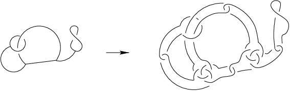
The surgery of along is called a surgery along , and the manifold is denoted by . We call two clovers and in surgery equivalent, and denote , if is diffeomorphic to .
Denote by the connected components of . For an –tuple we put
where and . If the degree of each is 1, we recover the definition of for Y–links.
Suppose that a leaf or a cycle of edges of in bounds an embedded surface in . Then the intersection number of its push-off along the framing with does not depend on the choice of and (by a slight abuse of terminology) will be also called the framing of this leaf or cycle. A leaf is trivial, if it is 0–framed and bounds a disc in whose interior does not intersect .
Lemma 2.2.
Let be a connected clover, which contains a trivial leaf . Then surgery on preserves a neighborhood of , where is the disc bounding . In particular, and :
![[Uncaptioned image]](0005192v4/disc.png)
|
Proof.
Follows from the construction of by an application of . ∎
An edge of a clover is a trivial loop, if both its endpoints coincide, it is 0–framed, and bounds a disc whose interior does not intersect .
Lemma 2.3.
Let be a connected clover, which contains a trivial looped edge . Then surgery on preserves a neighborhood of , where is the disc bounding . In particular, and .
Proof.
Follows from the construction of by an application of :
![[Uncaptioned image]](0005192v4/loop.png)
|
∎
Theorem 2.4.
Let be a clover in , and let be obtained from by cutting an internal edge of and inserting there two small Hopf-linked leaves:
![[Uncaptioned image]](0005192v4/edgecut.png)
|
Then and , where the sign is negative if the edge is splitting , and positive otherwise.
Proof.
The equality follows from the construction of by an application of . Topologically, this corresponds to cutting the corresponding solid handlebody introducing a pair of complimentary handles as shown below:
![[Uncaptioned image]](0005192v4/edgecut2.png)
|
Let be the component of containing this edge, and , be the components of replacing . Note that each subclover of which contains exactly one of the components and , has a trivial leaf. Thus by the definition of and Lemma 2.2 if has the same number of components as , and otherwise. ∎
Corollary 2.5.
Let be a degree clover. Then .
3 Topological calculus of clovers
Below we describe some important moves – on Y–links, which are shown to preserve the surgery equivalence classes. One can apply these moves also to clovers, in view of Theorem 2.4.
Moves and (similar to the Kirby moves , ) are shown in Figure 6:
- :
Add to a connected clover , which has a 0–framed leaf bounding an embedded disc whose interior does not intersect .
- :
Add a leaf to another leaf of the same Y–graph along a band by replacing with , where is a push-off of along the framing; then change the framing by .

Let be a leaf of a Y–graph and be the adjacent edge. Let be a knot. The move is sliding an edge along , see Figure 7:
- :
Denote by Y–graph obtained from by adding to along a band . Construct a Y–graph as shown in Figure 7: one of its leaves is a push-off of (and the adjacent edge goes along ), another is a push-off of , and the third leaf is a 0–framed unknot linked once with . Replace by .

Let be a leaf of a Y–graph , , and be its edges, with adjacent to . An arc , starting at and ending on , cuts into two parts and . The move is cutting the leaf along , see Figure 7:
- :
Let be an Y–graph obtained from by replacing the leaf by . Let be obtained from by replacing the leaf by , adding to along the band , and taking a push-off copy , as shown in Figure 7. Replace by .
A convenient way to draw the moves – is by depicting them in a standard handlebody, which then can be embedded into a manifold in an arbitrary way. Below is such an interpretation of the moves , as moves in a standard handlebody of genus 4:

For example, when the handlebody is embedded so that one of the handles links another handle as in Figure 9a, the corresponding move is shown in Figure 9b.

Theorem 3.1.
The moves – preserve the classes of surgery equivalence of Y–links in a manifold .
Proof.
It suffices to prove the surgery equivalence of Y–links obtained by the moves – in the standard handlebody. Instead of drawing the handlebodies we will draw thick lines passing through the handles (encoding a set of surgery and clover components), similarly to Lemma 2.1.
![[Uncaptioned image]](0005192v4/slidepf.png)
![[Uncaptioned image]](0005192v4/linkpf.png)
![[Uncaptioned image]](0005192v4/cutpf.png)
The following theorem was announced in [Gu2] in case of a Y–graph .
Theorem 3.2.

Proof.
Let us first verify the statement for a Y–graph. By an isotopy and a subsequent application of and , we get
![[Uncaptioned image]](0005192v4/inversep.png)
|
The general case now follows by Theorem 2.4. Finally, by . ∎
4 The structure of the graded spaces
This section is devoted to the study of the graded spaces
Denote iff .
4.1 Graded versions of –
Corollary 4.1.
Let be a clover of degree in a manifold , and let be obtained from by sliding one of its leaves along an adjacent leaf by . Then , and hence .
Let be a Y–graph in , and let be obtained from by an application of , see Figure 7. Note that by , thus
Hence, using Theorem 2.4 we obtain:
Corollary 4.2.
Let be a clover of degree in a manifold , and let be a knot. Let be obtained from by sliding an edge of along . Then .
In Lemma 4.10 we will strengthen this result by computing the difference in .
Let be a Y–graph in , and let be obtained from by an application of , see Figure 7. By the previous Lemma, the value of in does not change when we slide its edge along a knot. Thus we can pull off , making it back into . Hence, using again Theorem 2.4 we obtain:
Corollary 4.3.
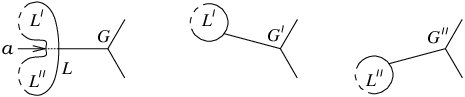
Let be a clover of degree in a manifold and be a leaf of . An arc starting in the external vertex incident to and ending in other point of , splits into two arcs and . Denote by and the clovers obtained from by replacing the leaf with and respectively, see Figure 11. Then .
4.2 The dependence on framings
Theorem 3.2 allows us to deduce the dependence of on the framings of edges.
Lemma 4.4.
Let be a clover of degree in a manifold . Let be obtained from by twisting the framing of an edge by a half twist. Then .
Proof.
Let and be the Y–graphs depicted in Figure 10b. Note that looks exactly like , except for the way its lower leaf links the thick line. Turning this leaf to the same position changes the framing of the adjacent edge by a half twist:
![[Uncaptioned image]](0005192v4/twistpf.png)
|
By Theorem 3.2, ; also, and by Lemma 2.2. Thus
and the lemma follows.
Corollary 4.5.
Let be a clover of degree in . Adding a kink, ie, a full twist to the framing of an edge preserves an –equivalence class of .
Now, note that the following two Y–graphs are isotopic:
![[Uncaptioned image]](0005192v4/orderpf.png)
|
Corollary 4.6.
Let and be clovers of degree in a manifold , which coincide everywhere except for a fragment shown in Figure 12. Then .

4.3 Simplifying the leaves
Denote by . We want to show that the space is generated by clovers with only internal vertices, ie, without leaves.
A leaf of a clover is special, if it is –framed and bounds an embedded disc, whose interior does not intersect . A leaf of a clover is simple, if it either bounds an embedded –framed disc whose interior intersects in at most one point, or is special.
For , the graded space is generated by clovers of degree all leaves of which are simple. Indeed, suppose we are given an arbitrary clover of degree in . We may split each of its non-trivial leaves into small pieces and apply Corollary 4.3 to present in as a linear combination of clovers with simple leaves.
Suppose that all leaves of clover in a manifold are simple. If two simple leaves are linked with each other (see Figure 13a), we replace them by a new edge by Theorem 2.4. Suppose that at least one simple leaf still remains after this procedure. We will show below that in this case .
We should consider three cases, see Figure 13b–d. Firstly, it may be that is trivial. Secondly, it may be that is 0–framed, and the disc intersects an edge of . Thirdly, it may be that is special.

In the first case, by Lemma 2.2. The second case can be reduced to the first case after unlinking the edge from the corresponding leaf by Corollary 4.2 (sliding the edge along a small unknot linked once with the leaf). Thus we readily obtain:
Lemma 4.7.
Let be a clover of degree in a manifold . Suppose that contains a 0–framed leaf bounding an embedded disc, whose interior intersects in exactly one point, belonging to an edge. Then .
In the third case we encounter 2–torsion.
Lemma 4.8.
Let be a clover of degree in a manifold , which contains a special leaf. Then .
Proof.
Rotating the special leaf we can change the framing of the adjacent edge while preserving the isotopy class of . Thus by Lemma 4.4 and the lemma follows. ∎
Over the integers, we have the following inclusion:
Lemma 4.9.
Let and be as in Lemma 4.8. Suppose that the connected component of which contains is of degree at least two. Then .
Proof.
Cutting the neighboring internal edge we obtain two new leaves and . Without a loss of generality suppose that the framing of is . Then slide along by as shown below:
![[Uncaptioned image]](0005192v4/fragmpf1.png)
|
Notice that changes the framing of a leaf by , so the new leaf is 0–framed. Splitting as shown above by Corollary 4.3, we obtain two clovers each of which contains a trivial leaf (either or ), and so can be removed by . ∎
4.4 The IHX relation
Let be an –component Y–link which contains a Y–graph , and let be a knot in . Choose a band connecting an edge of to . Sliding this edge of along by , we obtain a Y–graph , as shown in Figure 7. Denote . By Corollary 4.2, . There is a simple expression for this difference modulo . It is easier to visualize the picture in a neighborhood of , which is a genus 4 handlebody embedded into .
Lemma 4.10.
Let , and be the clovers of Figure 14 in a handlebody embedded into . Let be a degree clover in the complement of . Put , and . Then .

Here is another graphical expression for the above graphs:
![[Uncaptioned image]](0005192v4/slide2.png)
|
Proof.
![[Uncaptioned image]](0005192v4/slide2pf.png)
Theorem 4.11.
Let , and be clovers of degree in a manifold , which coincide everywhere except for a fragment shown in Figure 15. Then .

Proof.
It suffices to prove the statement for ; the general case then follows by Theorem 2.4 and Lemma 2.2. Consider a standard Y–graph in a handlebody of genus 3 and attach to an additional handle . We are to slide all three edges of along in a genus 4 handlebody as indicated in Figure 16. Each time we will use Lemma 4.10 to compute the corresponding change of .

Sliding the first edge of , we obtain a new Y–graph with . Sliding the next edge of (or rather of ), we obtain a new Y–graph with . After sliding the third edge we return back to and get . Here a degree 2 clovers , , and are shown in Figure 17.

Summing up these three equalities we get
| (1) |
But differs from only by an edge slide, and differs from by an edge slide and a cyclic ordering of edges in a vertex, see Figure 17. Hence by Corollary 4.2, and by Corollaries 4.2 and 4.6. A substitution of two these expressions into (1) proves the theorem. ∎
Remark 4.12.
There is a topological version of the IHX relation, which may be deduced similarly using the and moves to slide each edge of a Y–graph through a handle in a handlebody of genus 4. We leave the details to an interested reader.
4.5 Trivalent graphs and
Consider an abelian group freely generated by abstract (not necessarily connected) trivalent graphs with vertices and without looped edges, equipped with a cyclic ordering of the incident edges in each vertex. Denote by the quotient of by the following AS and IHX relations:
Denote by a Y–graph in with three special leaves. For each graph pick an arbitrary embedding of into . Equip it with a framing so that the framing along each cycle of edges is integer, and take its disjoint union with copies of . The resulting framed graph in may be considered as a clover of degree . Denote it by . Put and extend to by linearity. Note that by Corollary 2.5.
Theorem 4.13.
The map induces a quotient map , which is surjective and does not depend on the choice of . The image of is a 2–torsion.
Proof.
Note that , hence consists of a 2–torsion and we obtain:
Corollary 4.14.
For any , .
5 The equivalence of the , and filtrations
5.1 Equivalence of and
We can present surgery on an arbitrary blink of genus as surgery on blinks of genus one, slicing the surface into pieces of genus one as shown below (see also [GL]):
![[Uncaptioned image]](0005192v4/genus.png)
|
Also, as noticed already in [Ma], surgery on a blink of genus one can be presented as Y–surgery (and vice versa). Indeed, depicting the Borromean linking with one component passing on the boundary of an embedded surface with two bands, and then using , we obtain:
Lemma 5.1.
![[Uncaptioned image]](0005192v4/blink.png)
|
Therefore the following theorem holds:
Theorem 5.2.
For each integer we have .
5.2 Comparison of and : plan of the proof
The rest of the section is arranged in the following way.
We will first present any Y–link of degree by a trivial –component Y–link in , together with a trivial unimodular link which links in a special way. We shall then prove an inclusion by an easy counting argument.
The opposite inclusion is similar in spirit. Now we present any –component algebraically split link by a trivial link , together with a trivial Y–link linking in a special way. We then consider an appropriately modified version of some results of Section 4. Building on these results, we prove the inclusion using a similar counting argument.
5.3 Undoing Y–graphs
A link in laces a clover , if is trivial unimodular, and each of the (pairwise disjoint) discs bounding its components intersects in at most two points, which belong to the leaves of . A Y–link in is trivial, if it consists of Y–graphs standardly embedded in disjoint balls.
Lemma 5.3.
Let be a trivial –component Y–link in . For any –component Y–link in , there exists a link in which laces , such that .
Proof.
Any Y–link in , in particular , can be made into a trivial Y–link by framing twists and crossing changes. Moreover, it suffices to use crossing changes which involve only the leaves of Y–graphs. Indeed, instead of a crossing change which involves an edge of a Y–graph, one can do two subsequent crossing changes with the neighboring leaf of this graph (by sliding first the other branch towards the leaf). Using we can realize each of these framing and crossing changes by surgery on a trivial unimodular surgery link, as illustrated in Figure 3. The resulting collection of these surgery components comprises . ∎
For a Y–link in a manifold and a link denote by the double alternating sum:
Corollary 5.4.
The space is generated by all , where is a trivial Y–link in of degree at least , and the link laces .
Proof.
By Lemma 5.3, is generated by all , with and as above. It remains to notice that and that any sublink of also laces . ∎
Theorem 5.5.
For each integer we have .
Proof.
Let be a trivial Y–link in of degree at least and be an arbitrary link lacing . In view of Corollary 5.4, it suffices to prove that belongs to . Suppose that some leaf of is not linked with , ie, bounds a disc which does not intersect ; then by Lemma 2.2. Otherwise, all (ie, at least ) leaves of are linked with . But each component of is linked with at most two leaves of ; hence the number of components of is at least . Therefore . ∎
5.4 Undoing an AS–link
Let be a framed link in . We call an AS–link, if it is algebraically split and unimodular. In Section 5.3 above we presented any Y–link by a trivial Y–link , together with a trivial unimodular link lacing it. In this section we shall do the opposite: we present any AS–link by a trivial unimodular link , together with a trivial Y–link linking it in a special way, which we will also call “lacing”.
A clover in laces a link , if each leaf of either is trivial and links once (ie, bounds a disc which intersects in one point), or is unlinked with (ie, bounds a surface which does not intersects ).22 2 In fact, we will not need this type of leaf, but prefer to formulate the definition in its full generality A pair consisting of a trivial link in and a Y–link lacing is called a lacing pair. A lacing pair is trivial, if is trivial. Surgery on a trivial lacing pair in was called a Borromean surgery in [Ma] and a –move in [MN]. It was shown in [Ma, MN], that one can pass from a link in to any other link with the same linking matrix by surgery on a trivial Y–link lacing . Applying this result to AS–links, we deduce:
Lemma 5.6.
Let be a trivial unimodular –component link in a . For any AS–link in , there exists a trivial lacing pair , such that .
Corollary 5.7.
The space is generated by all , where is a trivial unimodular link in with at least components and a trivial Y–link laces .
Proof.
By Lemma 5.6, is generated by all , with and as above. It remains to notice that and that any Y–sublink of also laces . ∎
In what follows, we will in fact need only a weaker version of Corollary 5.7, in which we omit the assumption of triviality of the lacing pair.
5.5 The inclusion
We will need a modification of Corollary 4.2 and Lemma 4.4. Returning to their proofs, we notice that both statements can be stated for Y–links lacing a fixed link in :
Corollary 5.8.
Fix a link in a manifold . Let be a Y–link of degree lacing and let be obtained from by sliding an edge of along a knot . Suppose that for every Y–link of degree lacing one has . Then .
Lemma 5.9.
Fix a link in a manifold . Let be a Y–link of degree lacing and let be obtained from by twisting the framing of some edge by a half twist. Suppose that for every Y–link of degree lacing one has . Then
Moreover, the following version of Lemma 4.8 holds:
Lemma 5.10.
Let be a lacing pair in a manifold with of degree . Suppose that some disc bounding a component of intersects in just one point, which belongs to a leaf of . Suppose also that for any lacing pair with of degree greater than we have . Then .
Proof.
We are in a position to prove the second inclusion theorem.
Theorem 5.11.
For each integer we have .
Proof.
Let be a lacing pair in with having at least components. In view of Corollary 5.7, it suffices to prove that . We proceed by downward induction on the degree of . If , then obviously and the theorem follows. Suppose now that the inclusion holds for all Y–links of degree higher than and let us prove it for a Y–link of degree .
By a repeated use of Corollary 5.8 we can reduce the problem to the case when none of the edges of pass through the discs bounding the components of .
If for some the disc does not intersect , then by Lemma 2.2, and we are done.
If some disc intersects in exactly one point belonging to a leaf of , the statement follows from Lemma 5.10 (applicable by the induction assumption).
We are left with the case when each component of is linked with at least two leaves of . But each leaf of can be linked with at most one component of . Therefore, should have at least leaves, ie, at least components. Hence , and the theorem follows. ∎
Remark 5.12.
Over the integers, a simplified version of the above counting argument leads to an inclusion that does not require Lemmas 5.9 and 5.10. Indeed, we proceed as in the proof of Theorem 5.11 above, first reducing the problem to the case when no edges of pass through the discs , and then noticing that if some does not intersect , then by Lemma 2.2. Otherwise, each of the discs intersects at least one leaf of . Each leaf of can intersect at most one disc, so should have at least leaves, ie, at least components, hence .
6 The equivalence of the and filtrations
6.1 Plan of the proof
The section is arranged in the following way.
In the first part we shall prove an inclusion . This is done in two steps. By Corollary 5.4 the space is generated by all , where is a trivial –component Y–link in , and the link laces . In the first step, we take , construct a “good” sublink with at least components, and show that this implies . Building on this result, in the second step we prove a stronger inclusion using the IHX relation.
In the second part we shall prove an opposite inclusion . We present any –component boundary link as an image of a trivial unimodular link under surgery on a Y–link , linking in a special way, which we will call “1–lacing”. Using this presentation together with an appropriately modified version of Lemma 5.10, we prove that by an easy counting argument.
6.2 Constructing a boundary sublink
Let be a trivial component Y–link in and let be a link which laces . Below we construct a sublink with at least components, which will be a boundary link in the manifold, obtained from by surgery on . This construction is based on a notion of a good sublink.
A link in is good, if laces and the following conditions hold:
- •
No Y–graph of is linked with by all three leaves.
- •
If some Y–graph of is linked with by two leaves, then it is linked with just one component of .
The possible structure of in a neighborhood of a component of is shown in Figure 18.

Lemma 6.1.
Let be a trivial Y–link in and be a good sublink. Then the image of in is a boundary link in a neighborhood of , where is a union of discs bounding the components of .
Proof.
Cut out a tubular neighborhood of ; this is a disjoint union of genus 3 handlebodies. Components of bound non-intersecting discs in , which intersect the boundary by either one or two circles, which are meridians of . Perform surgery on by cutting, twisting by an appropriate element of the mapping class group, and gluing back the handlebodies . This transforms the meridians into some other curves on . It suffices to show that for each handlebody of these curves on are bounding inside .
Let be a meridian on . The surgery on this Y–graph corresponds to the action of an element of the Torelli subgroup (which acts trivially on ), so the image of still bounds a surface . Now, recall that is a good link, so there are only two possible configurations of the meridians. Firstly, may contain just two meridians and , corresponding to the same component of . Then, smoothing the intersections of with , we obtain a surface bounding . Secondly, these meridians may appear only on one of the three handles of . Pick one of the meridians ; all other meridians on may be considered as small push-offs of in the normal direction. Thus their images under the Y–surgery, together with the corresponding surfaces, can be obtained by a similar push-offs. This finishes the proof of the lemma. ∎
Corollary 6.2.
Let be a trivail Y–link in and be an –component good link with the union of discs bounding . Then for any link in .
Proof.
By Lemma 6.1, the image of B under surgery on bounds in the complement of . Thus it will bound also in , for any . ∎
Lemma 6.3.
Let be a trivial –component Y–link in and let be a link, which laces and links all leaves of . Then there exists a good sublink of with at least components.
We will say that two components of (respectively, two leaves of ) are neighboring, if there is a Y–graph (respectively, a component of ) which is linked with both of them.
Proof.
Suppose that there is a leaf of , which has at least neighbors, apart from the other leaves of the same Y–graph. Then the corresponding components of comprise . It remains to consider the case when each leaf of has less than neighbors belonging to other Y–graphs. Pick an arbitrary component of and remove from all neighboring components of . Repeat this step, each time picking a new component of the remaining link, until there are no more components left. Finally, take .
Let us establish a lower bound for the number of these steps. Each is linked with at most two Y–graphs, leaves of which have altogether at most other neighboring leaves. Thus the removal of and of the link components neighboring may unlink at most leaves of . In the beginning, was linked with all leaves of . Therefore, the number of steps is at least , thus has more than components. ∎
Remark 6.4.
In fact, one can assume that the degree of is just , but the construction of in this case is significantly more complicated.
6.3 The inclusion
Let us start with a weaker inclusion:
Proposition 6.5.
For each integer , we have .
Proof.
Let be a trivial –component Y–link in and be an arbitrary link lacing . In view of Corollary 5.4, it suffices to prove that . If some leaf of is not linked with , then . Otherwise, all leaves of are linked with and we can use Lemma 6.3 to find a good sublink of with at least components. It remains to apply Lemma 6.1 for and . ∎
Now we are in a position to prove a stronger result:
Theorem 6.6.
For each integer , we have .
Proof.
Let be a clover of degree in . We proceed by the downward induction on . If , then by Proposition 6.5, and the theorem follows. Suppose that the statement holds for any clover of degree higher than , and let us prove it for a clover of degree . Note that by the induction assumption we can use Theorem 4.13. Thus it suffices to prove the statement for a clover which is a disjoint union of a degree clover with no leaves and copies of a Y–graph with three special leaves.
We call a path in a connected graph maximal, if it is connected, passes along each edge at most once, and contains the maximal number of edges. A path in is maximal, if it is maximal in each of its connected components. The number of vertices of which do not belong to a maximal path is called the length-defect of . If is positive, pick a vertex of which does not belong to a maximal path, but is connected to it by an edge. Applying to this edge the IHX relation of Theorem 4.11, we obtain two clovers, each of which has the length defect . Hence it suffices to prove the theorem for . Notice that if , there are at least edges of without common ends. Thus, including ’s, there are at least edges of without common ends.
Cut all edges of by Theorem 2.4. Now, unlink all pairs of newly created leaves and change the framing of all leaves of ’s to 0 by , as shown below:
![[Uncaptioned image]](0005192v4/reduce.png)
|
Denote by the resulting link and by the –component Y–link obtained from . Clearly the link laces and
We should show that for each . If some leaf of is unlinked with , then this leaf is trivial and . Otherwise, by the construction of , there are at least non-neighboring components of (since there were at least edges of without common ends). These components comprise a good sublink of . The theorem now follows from Corollary 6.2. ∎
6.4 Undoing a boundary link
Let be a boundary link in , and fix a surface bounded by . We would like to present by a trivial unimodular link bounding a collection of discs, together with a Y–link, lacing it in a rather special way. Namely, we will say that a Y–link –laces the link , and each of its components intersects in at most one point, which belongs to a trivial leaf. By the classification of surfaces, we can assume that a surface bounding each component is an embedding of a connected sum of discs with two attached bands. Lemma 5.1 shows how such a disc with two (possibly linked and knotted) bands can be obtained from a standard disc by surgery on a Y–graph –lacing it:
![[Uncaptioned image]](0005192v4/admissib.png)
|
A pair consisting of a trivial link and a Y–link in is called a –lacing pair, if –laces for being discs bounding the components of . Exchanging pairs of bands to –lacing Y–graphs (or vice versa) as above, we obtain
Corollary 6.7.
For any –component boundary link in a manifold there exists a –lacing pair such that surgery on transforms into . Conversly, for any –lacing pair , surgery on transforms into a boundary link.
We illustrate this construction on an example of a genus 2 surface bounding a trefoil:
![[Uncaptioned image]](0005192v4/trefoil.png)
|
Remark 6.8.
A presentation of a boundary link by a –lacing pair encodes an information about the Seifert surface of and the Seifert form. Indeed, each Y–graph of corresponds to a pair of bands, ie, to a handle of . The cores , of these bands, being appropriately oriented and closed in the disc in a standard way, comprise a preferred basis of . This observation allows one to deduce that the Seifert matrix is given by , where is the linking matrix of non-trivial leaves of . We will investigate some applications of this construction in a future paper.
Corollary 6.9.
The space is generated by all , where is a –lacing pair in and has at least components.
Proof.
By Corollary 6.7, is generated by all , with and as above. It remains to notice that , and that any Y–sublink of also –laces . ∎
6.5 The inclusion
Returning to the proof of Lemma 5.10 (and Lemmas 5.9, 4.4 used in it), we notice that it may be restated for –lacing pairs in . Thus the following modified version of Lemma 5.10 holds:
Lemma 6.10.
Let be a –lacing pair in a manifold with of degree . Suppose that some disc bounding a component of intersects in just one point. Suppose also that for any –lacing pair with of degree greater than we have . Then .
We are ready to prove the last inclusion theorem.
Theorem 6.11.
For each integer we have .
Proof.
Let be a –lacing pair in such that has at least components. We will show by downward induction on the degree of that . If , then obviously . Inductively suppose that the statement holds for any –lacing pair in with of degree greater than .
If for some the disc bounding a component of does not intersect , then obviously and we are done. If for some the disc intersects in exactly one point, the statement follows from Lemma 6.10 (applicable by the induction assumption). We are left with the case when each disc intersects in at least two points. Since –laces , these points should belong to the leaves of different Y–graphs, which do not intersect any other disc , . Therefore, should have at least components, and the theorem follows. ∎
Remark 6.12.
The inclusion of Theorem 6.11 and its proof are valid not just for HS, but for arbitrary 3–manifolds.
References
- [1]
- [CM] T D Cochran, P M Melvin, Finite type invariants of 3–manifolds, Rice University and Bryn Mawr College preprint, November 1997, available from arxiv:math.GT/9805026
- [Ga] S Garoufalidis, On finite type 3–manifold invariants I, J. Knot Theory and its Ramifications, 5 (1996) 441–462
- [GL] S Garoufalidis, J Levine, Finite type 3–manifold invariants, the mapping class group and blinks, J. Diff. Geom. 47 (1997) 257–320
- [Gu1] M Goussarov, Knotted graphs and a geometrical technique of n–equivalence, St. Petersbourg Math. Journal, to appear, POMI preprint 1995 in Russian, available at http://www.ma.huji.ac.il/drorbn/Goussarov,
- [Gu2] M Goussarov, Finite type invariants and –equivalence of –manifolds, Comp. Rend. Ac. Sci. Paris, 329 Série I (1999) 517–522
- [Ha] K Habiro, Claspers and finite type invariants of links, Geometry and Topology, 4 (2000) 1–83
- [Jo] D Johnson, An abelian quotient of the mapping class group, Math. Ann. 249 (1980) 225–242
- [Jo] D Johnson, A survey of the Torelli group, from “Low-dimensional topology (San Francisco, Calif. 1981)”, Contemporary Math. 20 (1983) 163–179
- [Ki] R Kirby, A calculus for framed links in , Invent. Math. 45 (1978) 35–56
- [Ma] S Matveev, Generalized surgeries of three-dimensional manifolds and representations of homology spheres, Mat. Zametki, 42 (1987) no. 2, 268–278; English translation in Math. Notices Acad. Sci. USSR, 42:2
- [MP] S Matveev, M Polyak, A geometrical presentation of the surface mapping class group and surgery, Comm. Math. Phys. 160 (1994) 537–556
- [MN] H Murakami, Y Nakanishi, On a certain move generating link-homology, Math. Ann. 284 (1989) 75–89
- [Oh] T Ohtsuki, Finite type invariants of integral homology 3–spheres, J. Knot Theory and its Ramifications, 5 (1996) 101–115