Vassiliev Invariants of Legendrian, Transverse, and Framed Knots in Contact -manifolds
Abstract.
We show that for a large class of contact -manifolds the groups of Vassiliev invariants of Legendrian and of framed knots are canonically isomorphic. As a corollary, we obtain that the group of finite order Arnold’s -type invariants of wave fronts on a surface is isomorphic to the group of Vassiliev invariants of framed knots in the spherical cotangent bundle of .
On the other hand we construct the first examples of contact manifolds for which Vassiliev invariants of Legendrian knots can distinguish Legendrian knots that realize isotopic framed knots and are homotopic as Legendrian immersions.
1. Introduction
In this section we describe the main results of the paper. (In case any of the terminology appears to be new to the reader, the corresponding definitions are given in the next section.)
If a contact structure on a -manifold is cooriented, then every Legendrian knot (i.e. a knot that is everywhere tangent to the contact distribution) has a natural framing (a continuous normal vector field). Hence when studying Legendrian knots in such contact manifolds the main question is to distinguish those of them that realize isotopic framed knots.
Similarly if the contact structure is parallelized, then every transverse knot (i.e. a knot that is everywhere transverse to the contact distribution) also has a natural framing, and when studying transverse knots in such contact manifolds again the main question is to distinguish those of them that realize isotopic framed knots.
Vassiliev invariants proved to be an extremely useful tool in the study of framed knots, and the conjecture is that they are sufficient to distinguish all the isotopy classes of framed knots. Vassiliev invariants can also be easily defined in the categories of Legendrian and of transverse knots. In this paper we study the relationship between the groups of Vassiliev invariants of these three categories of knots, and explore when these invariants can be used to distinguish Legendrian knots that realize isotopic framed knots.
Consider a contact manifold with a cooriented contact structure. Fix an Abelian group , a connected component of the space of framed immersions of into , and a connected component of the space of Legendrian immersions of into . We study the relation between the groups of -valued Vassiliev invariants of framed knots from and of -valued Vassiliev invariants of Legendrian knots from . The main results obtained in this paper are described below.
Theorem 1.
The groups of -valued Vassiliev invariants of Legendrian knots from and of framed knots from are canonically isomorphic, provided that the Euler class of the contact bundle vanishes on every realizable by a mapping .
Using Theorem 1 we show that:
Theorem 2.
The groups of -valued Vassiliev invariants of Legendrian knots from and of framed knots from are canonically isomorphic, provided that one of the following conditions holds:
- 1:
-
the contact structure is tight;
- 2:
-
the Euler class of the contact bundle is in the torsion of (in particular if the Euler class is zero).
- 3:
-
the contact manifold is closed and admits a metric of negative sectional curvature.
As a corollary, we get that for any surface the group of finite order Arnold’s -type invariants of wave fronts on is isomorphic to the group of Vassiliev invariants of framed knots in the spherical cotangent bundle of .
Previously the isomorphism of the groups of Vassiliev invariants of Legendrian and of framed knots was known only in the case where and is the standard contact (result of D. Fuchs and S. Tabachnikov [8]) or the standard contact solid-torus (result of J. Hill [14]). The proofs of these isomorphisms were based on the fact that for the -valued Vassiliev invariants of framed knots in these manifolds there exists a universal Vassiliev invariant also known as the Kontsevich integral. (Currently the existence of the Kontsevich integral is known only for a total space of an -bundle over a compact oriented surface with boundary, see the paper [2] of Andersen, Mattes, and Reshetikhin.)
Thus the approach used in [8] and [14] to show the isomorphism of the groups of Vassiliev invariants is not applicable for almost all contact -manifolds and Abelian groups and our results appear to be a strong generalization of the results of Fuchs, Tabachnikov and Hill.
We also construct the first examples where Vassiliev invariants can be used to distinguish Legendrian knots that realize isotopic framed knots and are homotopic as Legendrian immersions. These are also the first examples where the groups of Vassiliev invariants of Legendrian and of framed knots from the corresponding components of the spaces of Legendrian and of framed immersions are not canonically isomorphic.
Theorem 3.
The manifold admits infinitely many cooriented contact structures for which there exist Legendrian knots that can be distinguished by -valued Vassiliev invariants even though they realize isotopic framed knots and are homotopic as Legendrian immersions.
(See Theorem 4.1.1 and Theorem 4.2.2 in which the similar result is proved for any orientable total space of an -bundle over a nonorientable surface of a sufficiently high genus.)
For transverse knots we obtain the following result (see Theorem 3.2.2):
Theorem 4.
Let be a contact manifold with a parallelized contact structure, then the groups of -valued Vassiliev invariants of transverse and of framed knots (from the corresponding components of the spaces of transverse and of framed immersions) are canonically isomorphic.
2. Conventions and definitions.
In this paper is an Abelian group (not necessarily torsion free), and is a connected oriented -dimensional Riemannian manifold (not necessarily compact).
A contact structure on a -dimensional manifold is a smooth field of tangent -dimensional planes, locally defined as a kernel of a differential -form with non-vanishing . A manifold with a contact structure possesses the canonical orientation determined by the volume form . The standard contact structure in is the kernel of the -form .
A contact element on a manifold is a hyperplane in the tangent space to the manifold at a point. For a surface we denote by the space of all cooriented (transversally oriented) contact elements of . This space is the spherical cotangent bundle of . Its natural contact structure is the distribution of tangent hyperplanes given by the condition that the velocity vector of the incidence point of a contact element belongs to the element.
A contact structure is cooriented if the -dimensional planes defining the contact structure are continuously cooriented (transversally oriented). A contact structure is oriented if the -dimensional planes defining the contact structure are continuously oriented. Since every contact manifold has a natural orientation we see that every cooriented contact structure is naturally oriented and every oriented contact structure is naturally cooriented. A contact structure is parallelizable (parallelized) if the -dimensional vector bundle over is trivializable (trivialized). Since every contact manifold has a canonical orientation, one can see that every parallelized contact structure is naturally cooriented. A contact structure on a manifold is said to be overtwisted if there exists a -disk embedded into such that the boundary is tangent to while the disk is transverse to along . Not overtwisted contact structures are called tight.
A curve in is an immersion of into . (All curves have the natural orientation induced by the orientation of .) A framed curve in is a curve in equipped with a continuous unit normal vector field.
A Legendrian curve in a contact manifold is a curve in that is everywhere tangent to . If the contact structure on is cooriented, then every Legendrian curve has a natural framing given by the unit normals to the planes of the contact structure that point in the direction specified by the coorientation.
To a Legendrian curve in a contact manifold with a parallelized contact structure one can associate an integer that is the number of revolutions of the direction of the velocity vector of (with respect to the chosen frames in ) under traversing according to the orientation. This integer is called the Maslov number of . The set of Maslov numbers enumerates the set of the connected components of the space of Legendrian curves in (cf. 2.0.1).
A transverse curve in a contact manifold is a curve in that is everywhere transverse to . If the contact structure on is parallelized, then a transverse curve has a natural framing given by the unit normals corresponding to the projections of the first of the two coordinate vectors of the contact planes on the -planes orthogonal to the velocity vectors of the curve. A transverse curve in a contact manifold with a cooriented contact structures is said to be positive if at every point the velocity vector of the curve points into the coorienting half-plane, and it is said to be negative otherwise. There are two connected components of the space of transverse curves in , they consist of positive and negative transverse curves respectively. In general if is a contact manifold with a cooriented contact structure, then every connected component of the space of unframed curves contains two connected components of the space of transverse curves. They consist of positive and negative transverse curves respectively.
A knot (framed knot) in is an embedding (framed embedding) of into . In a similar way we define Legendrian and transverse knots in .
A singular (framed) knot with double points is a curve (framed curve) in whose only singularities are transverse double points. An isotopy of a singular (framed) knot with double points is a path in the space of singular (framed) knots with double points under which the preimages of the double points on change continuously.
An -valued framed (resp. Legendrian, resp. transverse) knot invariant is an -valued function on the set of the isotopy classes of framed (resp. Legendrian, resp. transverse) knots.
A transverse double point of a singular knot can be resolved in two essentially different ways. We say that a resolution of a double point is positive (resp. negative) if the tangent vector to the first strand, the tangent vector to the second strand, and the vector from the second strand to the first form the positive -frame. (This does not depend on the order of the strands). If the singular knot is Legendrian (resp. transverse), then these resolution can be made in the category of Legendrian (resp. transverse) knots.
A singular framed (resp. Legendrian, resp. transverse) knot with transverse double points admits possible resolutions of the double points. The sign of the resolution is put to be if the number of negatively resolved double points is even, and it is put to be otherwise. Let be an -valued invariant of framed (resp. Legendrian, resp. transverse) knots. The invariant is said to be of finite order (or Vassiliev invariant) if there exists a nonnegative integer such that for any singular knot with transverse double points the sum (with appropriate signs) of the values of on the nonsingular knots obtained by the resolutions of the double points is zero. An invariant is said to be of order not greater than (of order ) if can be chosen as the integer in the definition above. The group of -valued finite order invariants has an increasing filtration by the subgroups of the invariants of order .
2.0.1.
-principle for Legendrian curves. For a contact manifold with a cooriented contact structure, we put to be the total space of the fiberwise spherization of the contact bundle, and we put to be the corresponding locally trivial -fibration. The -principle proved for the Legendrian curves by M. Gromov ([12], pp.338-339) says that the space of Legendrian curves in is weak homotopy equivalent to the space of free loops in . The equivalence is given by mapping a point of a Legendrian curve to the point of corresponding to the direction of the velocity vector of the curve at this point. In particular the -principle implies that the set of the connected components of the space of Legendrian curves can be naturally identified with the set of the conjugacy classes of elements of .
2.0.2.
Description of Legendrian and of transverse knots in . The contact Darboux theorem says that every contact -manifold is locally contactomorphic to with the standard contact structure that is the kernel of the -form . A chart in which is contactomorphic to the standard contact is called a Darboux chart.
Transverse and Legendrian knots in the standard contact are conveniently presented by the projections into the plane . Identify a point with the point furnished with the fixed direction of an unoriented straight line through with the slope . Then the curve in is a one parameter family of points with (non-vertical) directions in .
A curve in is transverse if and only if the corresponding curve in is never tangent to the chosen directions along itself.
While a generic regular curve has a regular projection into the -plane, the projection of a generic Legendrian curve into the -plane has isolated critical points (since all the planes of the contact structure are parallel to the -axis). Hence the projection of a generic Legendrian curve may have cusps. A curve in is Legendrian if and only if the corresponding planar curve with cusps is everywhere tangent to the field of directions. In particular this field is determined by the curve with cusps.
3. Isomorphisms of the groups of Vassiliev invariants of Legendrian, of transverse, and of framed knots.
3.1. Isomorphism between the groups of order invariants of Legendrian and of framed knots
Let be a contact manifold with a cooriented contact structure. Let be a connected component of the space of Legendrian curves in , and let be the connected component of the space of framed curves that contains . (Such a component exists because a Legendrian curve in a manifold with a cooriented contact structure is naturally framed, and a path in the space of Legendrian curves corresponds to a path in the space of framed curves.) Let (resp. ) be the group of -valued order invariants of Legendrian (resp. framed) knots from (resp. from ). Clearly every invariant restricted to the category of Legendrian knots in is an element . This gives a homomorphism .
Theorem 3.1.1.
Let be a contact manifold with a cooriented contact structure. Let be a connected component of the space of Legendrian curves in , and let be the connected component of the space of framed curves that contains . Then the following two statements a and b are equivalent.
- a:
-
for any and any knots representing isotopic framed knots.
- b:
-
is a canonical isomorphism.
If the mapping from the isotopy classes of Legendrian knots in to the isotopy classes of framed knots in is surjective, then the proof of Theorem 3.1.1 is obvious. However in general this mapping is not surjective and the proof of Theorem 3.1.1 is given in Section 5.2. The famous Bennequin inequality shows that this mapping is not surjective even in the case where is the standard contact .
Theorem 3.1.1 implies that to obtain the isomorphism between the groups and it suffices to show that statement of Theorem 3.1.1 is true for the connected components and of the spaces of Legendrian and of framed curves.
3.1.2.
Condition . In [8] D. Fuchs and S. Tabachnikov showed that statement holds for all the connected components of the space of Legendrian curves when the ambient manifold is the standard contact and the group is . (One can verify that the proof of this Theorem of Fuchs and Tabachnikov goes through for being any Abelian group.) They later observed [9] that since their proof of this fact is mostly local, the similar fact should be true for a big class of contact manifolds.
However in fact the proof of their theorem is not completely local and is also based on the existence of well-defined Bennequin invariant and Maslov number for a Legendrian knot in . In general the Bennequin invariant is not well-defined unless the knot is zero-homologous and the Maslov number is not well-defined unless either the knot is zero-homologous or the contact structure is parallelizable. Thus the generalization of this Theorem to the case of manifolds other than meets certain difficulties. (And in fact the corresponding result does not hold for a big class of contact manifolds, see Section 4.)
By analyzing the proof of the Theorem of Fuchs and Tabachnikov (see Section 5.3) we get that it can be generalized to the case of an arbitrary contact -manifold with a cooriented contact structure, provided that the connected component (containing ) satisfies the following
Condition : the connected component of the space of framed curves contains infinitely many components of the space of Legendrian curves. (See Proposition 3.1.4 for the homological interpretation of condition .)
This generalization of the result of Fuchs and Tabachnikov and Theorem 3.1.1 imply the following Theorem.
Theorem 3.1.3.
Let be a contact manifold with a cooriented contact structure, and let be a connected component of the space of Legendrian curves in . Let be the connected component of the space of framed curves that contains . Let (resp. ) be the group of -valued order invariants of Legendrian (resp. framed) knots from (resp. from ). Then the groups and are canonically isomorphic, provided that satisfies condition .
Now we give a homological interpretation of condition .
Proposition 3.1.4.
Let be a contact manifold with a cooriented contact structure, let be the Euler class of the contact bundle, and let be a component of the space of framed curves in . Then does not satisfy condition if and only if there exists such that and is realizable by a mapping with the property that is a loop free homotopic to loops realized by curves from .
Remark 3.1.5.
Some immediate corollaries of Theorem 3.1.3 and the generalization of the Theorem of Fuchs and Tabachnikov about the isomorphism of the groups of the -valued Vassiliev invariants in the case of . Proposition 3.1.4 implies that if the contact structure is parallelizable (and hence the Euler class of the contact bundle is zero) then all the connected components of the space of framed curves satisfy condition . Applying Theorem 3.1.3 we conclude that for any Abelian group and for every connected component of the space of Legendrian curves and for the containing it component of the space of framed curves the groups and of -valued Vassiliev invariants are canonically isomorphic.
Clearly the value of the Euler class of the contact bundle is zero if is an integer homology sphere. Hence for any Abelian group we obtain the isomorphism of the groups and of -valued Vassiliev invariants. This generalizes the Theorem of D. Fuchs and S. Tabachnikov [8] saying that for the standard contact and for the quotient groups and are canonically isomorphic.
The proof of this Theorem of Fuchs and Tabachnikov was based on the fact that for the -valued Vassiliev invariants of framed knots in there exists the universal Vassiliev invariant constructed by T. Q. T. Le and J. Murakami [17]. (For unframed knots in the construction of the universal Vassiliev invariant is the classical result of M. Kontsevich [15], and the invariant itself is the famous Kontsevich integral.) The existence of the universal Vassiliev invariant is currently known only for a very limited collection of -manifolds, and only for being , , or . (Andersen, Mattes, Reshetikhin [2] proved its existence in the case where and is the total space of an -bundle over a compact oriented surface with .)
Remark 3.1.6.
Let be a contact manifold with a cooriented contact structure, and let be a connected component of the space of framed curves in . Theorem 3.1.3 implies that the group of -valued order invariants of Legendrian knots from a connected component of the space of Legendrian curves does not depend on the choice of a cooriented contact structure, provided that for this choice satisfies condition . And hence in these cases the group can not be used to distinguish cooriented contact structures on . (See Remark 3.1.5 and Theorems 3.1.8 and 3.1.10 for the list of cases when the connected components of the space of framed curves are known to satisfy condition .)
3.1.7.
Finite order Arnold’s -type invariants of wave fronts on surfaces. A very interesting class of contact manifolds satisfying the conditions of Theorem 3.1.3 is formed by the spherical cotangent bundles of surfaces with the natural contact structure on (see 2). The theory of the invariants of Legendrian knots in is often referred to as the theory of Arnold’s [1] -type invariants of fronts on a surface . The natural contact structure on is cooriented. (The coorientation is induced from the coorientation of the contact elements of .) One can verify that for orientable the standard contact structure on is parallelizable, and hence all the components of the space of framed curves satisfy condition . If is not orientable, then the standard cooriented contact structure on is not parallelizable, but one can still verify (cf. Proposition 8.2.4 [19]) that every connected component of the space of framed curves satisfies condition . Hence for any Abelian group and for any surface we obtain the canonical isomorphism of the groups of -valued order invariants of Legendrian and of framed knots (from the corresponding components of the spaces of Legendrian and of framed curves in with the standard contact structure). Or equivalently we get that the groups of -valued order -type invariants of fronts on and of -valued order invariants of framed knots in (from the corresponding components of the two spaces) are canonically isomorphic.
Previously it was known that for and the quotient groups and are canonically isomorphic. The proof of this result of J. W. Hill [14] was based on the fact that for the -valued Vassiliev invariants of framed knots in there exists the universal Vassiliev invariant constructed by V. Goryunov [11]. (For unframed knots in the existence of the universal Vassiliev invariant is the classical result of M. Kontsevich [15], and the invariant itself is the famous Kontsevich integral.) Our results generalize the result of J. W. Hill (even in the case of .
The following Theorem describes another big class of contact manifolds for which the groups of Vassiliev invariants of Legendrian and of framed knots (from the corresponding components of the two spaces of curves) are canonically isomorphic.
Theorem 3.1.8.
Let be a contact manifold (with a cooriented contact structure) such that , and for every mapping of the two-torus the homomorphism is not injective. Then all the components of the space of framed curves in satisfy condition , and hence the groups of -valued order invariants of Legendrian and of framed knots (from the corresponding components of the spaces of Legendrian and framed curves) are canonically isomorphic.
3.1.9.
The isomorphism of the groups of Vassiliev invariants in the case of closed manifolds admitting a metric of negative sectional curvature and other corollaries of Theorem 3.1.8.
Let be a closed manifold admitting a metric of negative sectional curvature. A well-known Theorem by A. Preissman (see [4] pp. 258-265) says that every nontrivial commutative subgroup of the fundamental group of a closed -dimensional manifold of negative sectional curvature is infinite cyclic. Hence for every mapping the kernel of is nontrivial. It is also known that the universal covering of such is diffeomorphic to , and hence . Thus every closed manifold admitting a metric of negative sectional curvature satisfies all the conditions of Theorem 3.1.8 and for an arbitrary cooriented contact structure on such we obtain the isomorphism of the groups of -valued order invariants of Legendrian and of framed knots from the corresponding components of the spaces of Legendrian and of framed curves.
Another important class of contact manifolds for which every connected component of the space of framed curves satisfies condition is formed by contact manifolds with a tight contact structure.
The following Theorem appeared as a result of discussions of Stefan Nemirovski and the author.
Theorem 3.1.10.
Let be a contact manifold with a tight cooriented contact structure. Then all the components of the space of framed curves in satisfy condition , and hence the groups of -valued order invariants of Legendrian and of framed knots (from the corresponding components of the spaces of Legendrian and framed curves) are canonically isomorphic.
3.2. Isomorphisms between the groups of Vassiliev invariants of transverse and of framed knots
Let be a contact manifold with a parallelized contact structure . Let be a connected component of the space of transverse curves in , and let be the connected component of the space of framed curves that contains . (Such a component exists because a transverse curve in a manifold with a parallelized contact structure is naturally framed, and a path in the space of transverse curves corresponds to a path in the space of framed curves.) Let (resp. ) be the group of -valued order invariants of transverse (resp. framed) knots from (resp. from ). Clearly every invariant restricted to the category of transverse knots in is an element . This gives a homomorphism .
Theorem 3.2.1.
Let be a contact manifold with a parallelized contact structure. Let be a connected component of the space of transverse curves in , and let be the component of the space of framed curves that contains . Then the following two statements a and b are equivalent.
- a:
-
for any and any knots representing isotopic framed knots.
- b:
-
is a canonical isomorphism.
Similar to the case of Theorem 3.1.1 the proof of Theorem 3.2.1 becomes obvious if the mapping from the isotopy classes of transverse knots in to the isotopy classes of framed knots in is surjective. However in general this mapping is not surjective and to obtain the proof of Theorem 3.2.1 one follows the ideas of the proof of Theorem 3.1.1 (The famous Bennequin inequality shows that this mapping is not surjective even for the standard contact .)
Thus to obtain the isomorphism between the groups and it suffices to show that statement of Theorem 3.2.1 is true for the connected components and of the spaces of transverse and of framed curves.
In [8] D. Fuchs and S. Tabachnikov showed that statement holds for all the connected components of the space of transverse curves in the case where is the standard contact and . (One can verify that the proof of this Theorem of Fuchs and Tabachnikov goes through for being any Abelian group.) They later observed [9] that since their proof of this fact is mostly local, the similar fact should be true for a big class of contact manifolds. However in fact the proof of their theorem is not completely local and is based on the existence of a well-defined Bennequin invariant for a transverse knot in . Unfortunately the Bennequin invariant is not well-defined unless the knot is zero homologous. And the generalization of this Theorem to the case of manifolds other than meets certain difficulties that are similar to the ones we meet when we generalize the analogous Theorem of Fuchs and Tabachnikov for Legendrian knots, see 5.3. We imitate the arguments we use in 5.3 and obtain that statement a of Theorem 3.2.1 is true for any contact -manifold with a parallelized contact structure. (Observe that in the case of transverse knots, on the contrary to the case of Legendrian knots, no extra conditions on the contact manifold appear to be needed for the statement a to be true.) Thus we get the following Theorem.
Theorem 3.2.2.
Let be a contact manifold with a parallelized contact structure, and let be a connected component of the space of transverse curves in . Let be the connected component of the space of framed curves that contains . Let (resp. ) be the group of -valued order invariants of transverse (resp. framed) knots from (resp. from ). Then the groups and are canonically isomorphic.
This generalizes the Theorem of D. Fuchs and S. Tabachnikov [8] saying that for the standard contact and for the quotient groups and are canonically isomorphic.
The proof of this Theorem of Fuchs and Tabachnikov was based on the fact that for the -valued Vassiliev invariants of framed knots in there exists the universal Vassiliev invariant constructed by T. Q. T. Le and J. Murakami [17]. (For unframed knots in the construction of the universal Vassiliev invariant is the classical result of M. Kontsevich [15], and the invariant itself is the well-known Kontsevich integral.) The existence of the universal Vassiliev invariant is currently known only for a very limited collection of -manifolds, and only for being , or . (Andersen, Mattes, Reshetikhin [2] proved its existence in the case where and is the total space of an -bundle over a compact oriented surface with .)
Thus the approach used in [8] to show the isomorphism of the quotient groups is not applicable for almost all contact -manifolds and Abelian groups , and Theorem 3.2.2 appears to be a strong generalization of the result of Fuchs and Tabachnikov.
Remark 3.2.3.
Let be a contact manifold with a parallelized contact structure, and let be a connected component of the space of framed curves in . Theorem 3.2.2 implies that for any the group of -valued order invariants of transverse knots from a connected component of the space of transverse curves contained in does not depend on the choice of a parallelized contact structure. Hence this group can not be used to distinguish parallelized contact structures on .
4. Examples of Legendrian knots that are distinguishable by finite order invariants.
In this section we construct a big class of examples when Vassiliev invariants distinguish Legendrian knots that realize isotopic framed knots and are homotopic as Legendrian curves. Theorem 3.1.1 says that in these examples the groups of Vassiliev invariants of Legendrian and of framed knots are not canonically isomorphic, and we obtain the first known examples when these groups are not canonically isomorphic.
Theorem of R. Lutz [16] says that for an arbitrary orientable -manifold every homotopy class of distributions of -planes tangent to contains a contact structure. (The Theorem of Ya. Eliashberg [6] says even more that every homotopy class of the distributions of -planes tangent to contains a positive overtwisted contact structure.)
However in our constructions we will use only the Euler classes of contact bundles. For this reason we start with the following Proposition.
Proposition 4.0.1.
Let be an oriented -manifold and let be an element of . Then can be realized as the Euler class of a cooriented contact structure on if and only if , for some .
4.1. Examples of nonisotopic Legendrian knots in that can be distinguished by Vassiliev invariants.
Let be a cooriented contact structure on such that the Euler class of the contact bundle is nonzero. (The Euler class takes values in , and Proposition 4.0.1 says that for any even there exists a cooriented contact structure on with the Euler class .)
Let be a knot in that crosses exactly once one of the spheres . The Theorem of Chow [3] and Rashevskii [18] says that there exists a Legendrian knot that is -small isotopic to as an unframed knot. Let be the Legendrian knot that is the same as everywhere except of a small piece located in a chart contactomorphic to the standard contact where it is changed as it is shown in Figure 1 (see 2.0.2).

Theorem 4.1.1.
- a:
-
Legendrian knots and belong to the same component of the space of Legendrian curves and realize isotopic framed knots.
- b:
-
There exists a -valued order one invariant of Legendrian knots, such that .
Remark 4.1.2.
Let , , be the knot that is the same as everywhere except of a small piece located in a chart contactomorphic to the standard contact where it is changed in the way described by the addition of zigzags shown in Figure 1. The Proof of Theorem 4.1.1 implies that all ’s are homotopic as Legendrian curves and realize isotopic framed knots, but for all Legendrian knots and are not Legendrian isotopic. The order one invariant of Legendrian knots constructed in the Proof of Theorem 4.1.1 has the property that . Hence this distinguishes all the ’s.
4.1.3.
Examples of nonisotopic Legendrian knots with overtwisted complements that realize isotopic framed knots and are homotopic as Legendrian immersions. Let be an embedded into disk centered at a point . The Theorem of Eliashberg [6] says that every homotopy class of distributions of -planes tangent to contains an overtwisted contact structure that has as the standard overtwisted disk. In the example of Theorem 4.1.1 we can start with an overtwisted contact structure that has as an overtwisted disk and with an unframed knot that is far away from . Then since both and were constructed using a -small approximation of , we can assume that they are also far away from . And we have constructed examples of nonisotopic Legendrian knots with overtwisted complements that realize isotopic framed knots and are homotopic as Legendrian immersions. Previously such examples were unknown and the Theorem of Ya. Eliashberg and M. Fraser [7] says that such examples are impossible if the ambient manifold is .
4.2. Examples of nonisotopic Legendrian knots in the total spaces of -bundles over nonorientable surfaces that can be distinguished by Vassiliev invariants.
4.2.1.
Below we describe another big family of examples where finite order invariants distinguish Legendrian knots that realize isotopic framed knots and are homotopic as Legendrian immersions.
Let be a nonorientable surface that can be decomposed as a connected sum of the Klein bottle and a surface . Let be an orientable manifold that admits a structure of a locally trivial -fibration . (For example one can take to be the spherical tangent bundle of .)
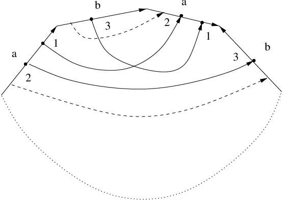
Consider an -fibration induced from by the mapping that corresponds to the solid loop in Figure 2. (In this Figure the enumeration of the end points of the arcs indicates which pairs of points should be identified to obtain the loop.) Since the solid loop is an orientation preserving loop in , we get that (torus). Put to be the natural mapping of the total space of the induced fibration into the total space of .
A homology class in projecting to the dashed loop in Figure 2 has intersection with the class realized by . Thus there exists such that . Proposition 4.0.1 says that for every the class is realizable as the Euler class of a cooriented contact structure on . Thus for every there exists a cooriented contact structure on such that the value of the Euler class of the contact bundle on is equal to .
Let be a cooriented contact structure on such that the Euler class of the contact bundle satisfies , for some nonzero .
Let be an arbitrary Legendrian knot such that its projection to (considered as a loop) is free homotopic to the solid loop in Figure 2. Let be Legendrian knots that are the same as everywhere except of a chart (contactomorphic to the standard contact ) where and are different from as it is described in Figure 3, see 2.0.2. (The number of cusps in Figure 3 is .)
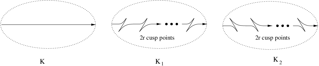
Theorem 4.2.2.
The knots and described above belong to the same component of the space of Legendrian curves and realize isotopic framed knots. There exists a -valued order one invariant of Legendrian knots from such that .
Remark 4.2.3.
Similarly to 4.1.3 one verifies that the contact structure and the knots and in the statement of Theorem 4.2.2 can be chosen so that the restrictions of the contact structure to the complements of and of are overtwisted.
Using the ideas of the Proof of Theorem 4.2.2 one can construct many other examples of Legendrian knots that can be distinguished by Vassiliev invariants of Legendrian knots even though they realize isotopic framed knots and are homotopic as Legendrian immersions. For example as a solid loop in Figure 2 we could take any loop such that the number of double points that separate into two orientation reversing loops is odd, and the value of the Euler class of the contact bundle on is nonzero.
5. Proofs
5.1. Useful facts, Lemmas, and some technical definitions
Proposition 5.1.1.
Let be a locally trivial -fibration of an oriented manifold over a (not necessarily orientable) manifold . Let be the class of an oriented -fiber of , and let be an element of . Then:
- a:
-
, provided that is an orientation preserving loop in .
- b:
-
, provided that is an orientation reversing loop in .
5.1.2.
Proof of Proposition 5.1.1. If we move an oriented fiber along the loop , then in the end it comes to itself either with the same or with the opposite orientation. It is easy to see that it comes to itself with the opposite orientation if and only if is an orientation reversing loop in .∎
Proposition 5.1.3.
Let be a surface (not necessarily compact or orientable), and let be a nontrivial commutative subgroup of . Then is infinite cyclic.
5.1.4.
Proof of Proposition 5.1.3. It is well-known that any closed , other than admits a hyperbolic metric. (It is induced from the universal covering of by the hyperbolic plane.) The Theorem of A. Preissman (see [4] pp. 258-265) says that if is a closed Riemannian manifold of negative sectional curvature, then any nontrivial Abelian subgroup is isomorphic to . Thus if is closed, then any nontrivial commutative is infinite cyclic. If is not closed, then the statement of the Proposition is also true because in this case is homotopy equivalent to a bouquet of circles. ∎
Proposition 5.1.5.
Let (Klein bottle) be a surface not necessarily closed or orientable. Let be an orientable -manifold, and let be a locally trivial -fibration. Let be the class of an oriented -fiber of , and let be an element with . Let be an element of the centralizer of . Then there exist and nonzero such that .
5.1.6.
5.1.7.
An important homomorphism. Let be a manifold, let be the space of free loops in , and let be a loop. An element is realizable by a mapping with . Let be the element corresponding to the trace of the point under the homotopy of described by . Let be the homomorphism that maps to .
Since the -cell of is glued to the -skeleton along the commutation relation of the meridian and of the longitude of , we get that is a surjective homomorphism of onto the centralizer of .
If for , then the mappings and of corresponding to these loops can be deformed to be identical on the -skeleton of . Clearly the obstruction for and to be homotopic as mappings of (with the mapping of the -skeleton of fixed under homotopy) is an element of obtained by gluing together the boundaries of the -cells of the two tori. In particular we get the Proposition of V. L. Hansen [13] saying that is an isomorphism, provided that .
5.1.8.
-principle for curves in . For a -dimensional manifold we put to be the manifold obtained by the fiberwise spherization of the tangent bundle of , and we put to be the corresponding locally trivial -fibration. The -principle (that can be found in [12]) says that the space of curves in is weak homotopy equivalent to (the space of free loops in ). The weak homotopy equivalence is given by mapping a curve to a loop that sends a point to the point of corresponding to the direction of the velocity vector of at .
Definition 5.1.9 (of and of ).
Let and be two framed knots that coincide pointwise as embeddings of . Then there is an integer obstruction for them to be isotopic as framed knots with the embeddings of fixed under the isotopy. This obstruction is calculated as follows. Let be the knot obtained by shifting along the framing and reversing the orientation on the shifted copy. Together and bound a thin strip. We put to be the intersection number of the strip with a very small shift of along its framing.
For a framed knot we denote by , , the isotopy class of a framed knot that coincides with as an embedding of and has .
For two singular framed knots and with transverse double points that coincide pointwise as immersions of , we put to be the value of on the nonsingular framed knots and that coincide pointwise as embeddings of and are obtained from and by resolving each pair of the corresponding double points of and of in the same way. (The value does not depend on the resolution as soon as the corresponding double points of the two knots are resolved in exactly the same way.) As before is the integer valued obstruction for and to be isotopic as singular framed knots with the immersion of corresponding to the two knots fixed under isotopy.
For a singular framed knot with transverse double points we denote by , , the isotopy class of a singular framed knot with transverse double points that coincides with as an immersion of and has .
Proposition 5.1.10.
Let and be framed knots (resp. singular framed knots with transverse double points) that coincide pointwise as embeddings (resp. immersions) of . Then and are homotopic as framed knots (resp. singular framed knots with transverse double points) if and only if is even.
5.1.11.
Proof of Proposition 5.1.10. Clearly if is even, then and are framed homotopic. (We can change the obstruction by two by creating a small kink and passing through a double point at its vertex.)
Every oriented -dimensional manifold is parallelizable, and hence it admits a -structure. A framed curve in represents a loop in the principal -bundle of . (The -frame corresponding to a point of is the velocity vector, the framing vector, and the unique third vector of unit length such that the -frame defines the positive orientation of .) One observes that the values of the -structure on the loops in the principal -bundle of realized by and are different provided that is odd. But these values do not change under homotopy of framed curves. Hence if is odd, then and are not framed homotopic. ∎
Definition 5.1.12 (of the number of framings of a knot).
Using the self-linking invariant of framed knots one can easily show that if and in 5.1.9 are pointwise coinciding zero-homologous framed knots and , then is not isotopic to in the category of framed knots. However for knots that are not zero-homologous this is not generally true, see 5.8.1. For this reason we introduce the following definitions.
If for an unframed knot there exist isotopic framed knots and that coincide with pointwise and have , then we say that admits finitely many framings. For that admits finitely many framings we put the number of framings of to be the minimal positive integer such that there exist isotopic framed knots and that coincide with pointwise and have . One can easily show that if admits finitely many framings, then there are exactly isotopy classes of framed knots realizing the isotopy class of the unframed knot . Proposition 5.1.10 implies that is even.
In a similar way we introduce the notion of the number of framings for unframed singular knots with double points.
Proposition 5.1.13.
Let be a contact -manifold with a cooriented contact structure, let be a connected component of the space of framed curves, and let be a connected component of the space of Legendrian curves in .
- a:
-
Let be an unframed knot obtained by forgetting the framing on a knot from . Then there exists a Legendrian knot from realizing the isotopy class of .
- b:
-
If is an isotopy class of framed knots in that is realizable by a Legendrian knot from , then the isotopy class of (see 5.1.9) is also realizable by a Legendrian knot from .
- c:
-
Let be an unframed singular knot with double points obtained by forgetting the framing on a singular knot from . Then there exists a singular Legendrian knot from realizing the isotopy class of .
- d:
-
If is an isotopy class of singular framed knots in that is realizable by a singular Legendrian knot from , then the isotopy class of is also realizable by a singular Legendrian knot from .
5.1.14.
Proof of statement a of Proposition 5.1.13. Let be the fiberwise spherization of the -dimensional contact vector bundle, and let be the corresponding locally trivial -fibration. We denote by the class of an oriented -fiber of . For a Legendrian curve denote by the loop in obtained by mapping a point to the point of corresponding to the direction of the velocity vector of at .
The -principle 2.0.1 says that Legendrian curves and in belong to the same component of the space of Legendrian curves in if and only if and are free homotopic loops in .
W. L. Chow [3] and P. K. Rashevskii [18] showed that every unframed knot is isotopic to a Legendrian knot (and this isotopy can be made -small). Deforming we can assume (see 5.1.8) that: 1: and coincide in the neighborhood of , 2: and realize the same element , and 3: that liftings to of Legendrian curves from are free homotopic to a loop in such that and .
Proposition 5.1.1 says that is in the center of , since the contact structure is cooriented and hence oriented. Then , for some .
Take a chart of (that is contactomorphic to the standard contact ) containing a piece of the Legendrian knot. From the formula for the Maslov number deduced in [8] it is easy to see that the modifications of the Legendrian knot corresponding to the insertions of two cusps shown in Figure 4 (see 2.0.2) induce multiplication by of the lifting of to an element of . (Here the sign depends on the choice of an orientation of the fiber used to define .) Performing this operation sufficiently many times we obtain the Legendrian knot from realizing the isotopy class of the unframed knot .

One easily modifies the arguments above to obtain the proof of statement c of Proposition 5.1.13.
Proof of statement b of Proposition 5.1.13. Take a chart of (that is contactomorphic to the standard contact ) containing a piece of the knot and perform the homotopy in shown in Figure 5, see 2.0.2. (Observe that a self-tangency point of the projection of a Legendrian curve in to the -plane corresponds to a double point of the Legendrian curve.) Straightforward verification (cf. the formula for the Bennequin invariant deduced in [8]) shows that the Legendrian knot we obtain in the end of the homotopy realizes .

5.2. Proof of Theorem 3.1.1
The fact that statement b of Theorem 3.1.1 implies statement a is clear. Thus we have to show that statement a implies statement b. This is done by showing that there exists a homomorphism such that and .
Let be an invariant. In order to construct we have to specify the value of on every framed knot .
5.2.1.
Definition of . If the isotopy class of the knot is realizable by a Legendrian knot , then put . The value is well-defined because if is another knot realizing , then by statement a of Theorem 3.1.1.
Let be the component of the space of unframed curves that corresponds to forgetting framings on the curves from . Propositions 5.1.13 and 5.1.10 imply that if an unframed knot admits finitely many framings (see 5.1.12), then all the isotopy classes of framed knots from realizing the isotopy class of the unframed knot are realizable by Legendrian knots from . Thus we have defined the value of on all the framed knots from that realize unframed knots admitting finitely many framings.
If admits infinitely many framings, then either 1) all the isotopy classes of framed knots from realizing the isotopy class of are realizable by Legendrian knots from or 2) there exists a knot realizing the isotopy class of such that is realizable by a Legendrian knot from and (see 5.1.9) is not realizable by a Legendrian knot from . (In this case etc. also are not realizable by Legendrian knots from , see 5.1.13.) In the case 1) the value of is already defined on all the framed knots from realizing . In the case 2) put
| (1) |
(Proposition 5.1.13 implies that the sum on the right hand side is well-defined.) Similarly put
Now we have defined on all the framed knots (from ) realizing . Doing this for all for which case 2) holds we define the value of on all the knots from .
Below we show that is an order invariant of framed knots from . We start by proving the following Proposition.
Proposition 5.2.2.
Let be a framed knot from , then defined as above satisfies identity (1).
5.2.3.
Proof of Proposition 5.2.2. If is not realizable by a Legendrian knot from , then the statement of the proposition follows from the formula we used to define .
If is realizable by a Legendrian knot , then consider a singular Legendrian knot with double points that are vertices of small kinks such that we get if we resolve all the double points positively staying in the class of the Legendrian knots. (To create we perform the first half of the homotopy shown in Figure 5 in places on .)
Let be the set of the possible resolutions of the double points of . For put to be the sign of the resolution, and put to be the nonsingular Legendrian knot obtained via the resolution . Since is an order invariant of Legendrian knots we get that
| (2) |
(Observe that if we resolve double points of negatively, then we get the isotopy class of .) This finishes the proof of the Proposition. ∎
5.2.4.
Let be a singular framed knot with double points. Let be the set of the possible resolutions of the double points of . For put to be the sign of the resolution, and put to be the isotopy class of the knot obtained via the resolution .
In order to prove that is an order invariant of framed knots from , we have to show that
| (3) |
for every .
First we observe that the fact whether identity (3) holds or not depends only on the isotopy class of the singular knot with double points.
If the isotopy class of is realizable by a singular Legendrian knot from , then identity (3) holds for , since is an order invariant of Legendrian knots (and the value of on a framed knot realizable by a Legendrian knot was put to be ).
Proposition 5.1.13 says that the isotopy class of the singular unframed knot obtained by forgetting the framing on is realizable by a singular Legendrian knot from .
If admits finitely many framings, then all the isotopy classes of singular framed knots from realizing the isotopy class of are realizable by singular Legendrian knots from , and we get that identity (3) holds for .
If admits infinitely many framings and all the isotopy classes of singular framed knots from realizing are realizable by singular Legendrian knots from , then (3) automatically holds for . If admits infinitely many framings but not all the isotopy classes of singular framed knots from realizing are realizable by singular Legendrian knots from . Then put to be the framed knot realizing that is realizable by a singular Legendrian knot from and such that , , are not realizable by singular Legendrian knots from .
Proposition 5.1.13 says that , , are realizable by singular Legendrian knots from and hence identity (3) holds for , . Using Proposition 5.2.2 and the fact that identity (3) holds for , , we show that (3) holds for . Namely,
| (4) |
Similarly we show that (3) holds for .
5.3. The reasons for the condition to appear
The proof of the Theorem of Fuchs and Tabachnikov that says that statement of Theorem 3.1.1 is true for all the connected components of the space of Legendrian curves when the ambient contact manifold is the standard contact is based on the following three observations:
- 1:
-
There are two types of cusps arising under the projection of the part of a Legendrian knot that is contained in a Darboux chart to the -plane (see 2.0.2). They are formed by cusps for which the branch of the projection of the knot going away from the cusp is locally located respectively above or below the tangent line at the cusp point, see Figure 4. For a Legendrian knot and we denote by the Legendrian knot obtained from by the modification corresponding to an addition of cusp pairs of the first type and cusp pairs of the second type to the projection of the part of located in a Darboux chart.
Let and be Legendrian knots in the standard contact that realize isotopic unframed knots. Then for any and large enough there exist such that the Legendrian knot is Legendrian isotopic to .
- 2:
-
If there exists such that Legendrian knots and are Legendrian isotopic, then every Vassiliev invariant of Legendrian knots takes equal values on and on .
- 3:
-
The number from the previous observation exists if the ambient contact manifold is and the Legendrian knots and belong to the same component of the space of Legendrian curves and realize isotopic framed knots.
The first two observation are true for any contact -manifold (since the proof of the corresponding facts is local). But the number from the statement of the third observation does not exist in general. In the case of the ambient manifold being Fuchs and Tabachnikov showed the existence of such using the explicit calculation involving the Maslov classes and Bennequin invariants of Legendrian knots. However in order for the Bennequin invariant to be well-defined the knots have to be zero-homologous, and in order for the Maslov class to be well-defined the knots have to be zero-homologous or the contact structure has to be parallelizable.
Below we show that such exists for any and that realize isotopic framed knots and belong to the same component of the space of Legendrian curves, provided that the connected component of the space of framed curves that contains and satisfies condition . (We assume that the contact structure on is cooriented.)
Let and be Legendrian knots as above, and let be such that and are Legendrian isotopic.
We start by showing that can be chosen so that , and that if satisfies condition , then .
5.3.1.
Proof of the fact that can be chosen so that . Let be the isotopy changing to in the category of framed knots. Analyzing the proof of Fuchs and Tabachnikov one verifies that for large enough the Legendrian isotopy changing to can be chosen so that for every the Legendrian knot is contained in a thin tubular neighborhood of and is isotopic (as an unframed knot) to inside .
For two framed knots and realizing unframed knots that are isotopic inside there is a well-defined -valued obstruction to be isotopic inside in the category of framed knots. This obstruction is the difference of the self-linking numbers of the inclusions of and into induced by an identification of with the standard solid torus in . (One verifies that for and that are isotopic as unframed knots inside this difference does not depend on the choice of the identification of with the standard solid torus in .)
From the formula for the Bennequin invariant stated in [8] one gets that the value of the obstruction for to be isotopic as a framed knot to inside is equal to . Similarly the value of the obstruction for to be isotopic as a framed knot to inside is equal to . Clearly the value of the obstruction for to be isotopic to inside does not depend on (for the isotopy changing to in the category of framed knots), and we get that .
5.3.2.
Proof of the fact that if satisfies condition , then . Let be the class of an oriented -fiber of . From the -principles for Legendrian and for unframed curves (see 2.0.1 and 5.1.8) one obtains that every component of the space of Legendrian curves contained in corresponds to the conjugacy class of , for some . (Connected components of the space of free loops in are naturally identified with the conjugacy classes of the elements of .)
Using Proposition 5.1.1 one verifies that if satisfies condition , then for every nonzero the elements and are not conjugate in .
From the formula for the Maslov number deduced in [8] and the -principle for Legendrian curves one gets that is contained in the component of the space of Legendrian curves that corresponds to the conjugacy class of . Using the fact that and are conjugate in (since and are Legendrian homotopic) and the fact that since the contact structure is cooriented is in the center of (see 5.1.1), we get that is contained in the component that corresponds to the conjugacy class of . Since and are Legendrian isotopic (and hence Legendrian homotopic) we get that and are conjugate in , and using 5.1.1 we get that is conjugate to . But since satisfies condition we have , and hence .
From the identities and one gets that and . Assume that . (The case where is treated similarly.) Put . It is easy to show that since and are Legendrian isotopic, then and are also Legendrian isotopic. (Basically one can keep the extra cusp pairs close together on a small piece of the projection of the part of the knot contained in a Darboux chart during the whole isotopy process.) But and are obtained from and by the modification corresponding to the addition of pairs of cusps of each of the two types, and we can take from the observation 2 to be .
This shows that and can not be distinguished by the Vassiliev invariants of Legendrian knots provided that satisfies condition , and that and realize isotopic framed knots and are homotopic as Legendrian immersions. Hence statement a of Theorem 3.1.1 is true provided that satisfies condition .
5.4. Proof of Proposition 3.1.4.
The -principle for curves 5.1.8 says that the set of the connected components of the space of curves in is naturally identified with the set of the connected components of the space of free loops in the spherical tangent bundle of . Hence it is also naturally identified with the set of conjugacy classes of the elements of . (From the long homotopy sequence of the fibration we see that it is also naturally identified with the set of conjugacy classes of the elements of .) Choose a -structure on . It is easy to see (cf. 5.1.10 and 5.1.11) that the set of the connected components of the space of framed curves in is identified with the product . Here the -factor is the value of the -structure on the loop in the principal -bundle of that corresponds to a framed curve from the connected component, see 5.1.11. (This value does not depend on the choice of the framed curve in the component.)
The -principle for the Legendrian curves says that the set of the connected components of the space of Legendrian curves is naturally identified with the set of homotopy classes of free loops in (the spherical contact bundle of ). Hence it is also naturally identified with the set of conjugacy classes of the elements of . Since every contact manifold is oriented and the contact structure was assumed to be cooriented, we get that the planes of the contact structure are naturally oriented. This orientation induces the orientation of the -fibers of . Put to be the class of the oriented -fiber of .
The Theorem of Chow [3] and Rashevskii [18] says that every connected component of the space of curves contains a Legendrian curve. Straightforward verification shows that the insertion of the zig-zag into the Legendrian curve (see Figure 4) changes the value of the -structure on the corresponding framed curve. It is easy to verify (see [8]) that the two connected components of the space of Legendrian curves that contain respectively and with the extra zigzag correspond to the conjugacy classes of and of (or of ) in . (We obtain or depending on which of the two possible zig-zags we insert.)
Let be a connected component of the space of Legendrian curves in that corresponds to the conjugacy class of . Then every connected component of the space of Legendrian curves corresponds to the conjugacy class of , for some .
Hence satisfies condition if and only if for every the elements and are not conjugate in .
Assume that does not satisfy condition , then there exists a nonzero and such that
| (5) |
This implies that and commute in . The commutation relation gives a mapping of the two-torus such that and .
Put to be the Euler class of the contact bundle. Consider the locally-trivial -fibration induced by from the -fibration . One can verify that is the Euler class of . On the other hand the Euler class of is and it is naturally identified with the value of on the homology class realized by . This implies that if does not satisfy condition , then there exists a homology class from the statement of the Proposition.
On the other hand the existence of the class from the statement of the Proposition implies that there exists a Legendrian curve such that is conjugate to , for being the value of (the Euler class of the contact bundle) on the homology class realized by . (Proposition 4.0.1 says that , for some , and hence is even.) This means that does not satisfy condition and we have proved Proposition 3.1.4. ∎
5.5. Proof of Theorem 3.1.8
5.5.1.
Let be the locally trivial -fibration introduced in 2.0.1 and let be the class of an oriented -fiber of .
Similar to 5.4 we get that to prove that all the components of the space of framed curves satisfy condition , it suffices to show that and are not conjugate in , for all and . Let and be such that
| (6) |
We have to show that .
Proposition 5.1.1 says that is in the center of . Hence
| (7) |
Identity (7) implies that and commute in . Hence there exists a mapping of the two-torus such that and . By the assumption of the Theorem has a nontrivial kernel. Thus there exist with at least one of and being nonzero such that , and hence
| (8) |
Since the situation is symmetric, we assume that .
Thus . Applying (7) to the last identity we get that . Since we see that has infinite order in , and hence . If is zero, then we are done. Hence we have to look at the case of . (We assumed that .) From (8) we get that , and hence by Proposition 5.1.1 is in the center of . Thus . On the other hand using (7) we get that . Since has infinite order in we get that . By our assumptions and we have . This finishes the proof of Theorem 3.1.8.∎
5.6. Proof of Theorem 3.1.10
By Theorem 3.1.1 it suffices to show that all the connected components of the space of framed curves in satisfy condition .
Let be the Euler class of the contact bundle of . Proposition 3.1.4 implies that it suffices to show that , for every homology class realizable by a mapping . The result of D. Gabai (see Corollary 6.18 [10]) implies that every realizable by a mapping of can be realized by a collection of spheres and of a torus that are embedded into . Finally the result of Ya. Eliashberg (see [5] Theorem ) says that for a tight contact structure the value of on any embedded torus or sphere is zero. Hence . This finishes the Proof of Theorem 3.1.10.∎
5.7. Proof of Proposition 4.0.1
First we show that if can be realized as the Euler class of the contact structure, then for some .
Since the contact structure is cooriented we get that the tangent bundle is isomorphic to the sum of the oriented contact bundle and the trivial oriented line bundle . The tangent bundle of every orientable -manifold is trivializable and we get that the second Stiefel-Whitney class of the contact bundle is zero. But the second Stiefel-Whitney of is the projection of the Euler class of under the natural mapping , and we get that for some .
Now we show that if , for some , then can be realized as the Euler class of a cooriented contact structure on .
Consider an oriented -dimensional vector bundle over with the Euler class . The second Stiefel-Whitney class of is zero, since it is the projection of . Since is an oriented vector bundle we have .
Consider the sum of with the trivial oriented -dimensional vector bundle . Clearly the total Stiefel-Whitney class of the -dimensional oriented vector bundle is equal to , and the Euler class of is equal to . Using the interpretation of the Stiefel-Whitney and the Euler classes of as obstructions for the trivialization of , we get that is trivializable. Since the tangent bundle of an oriented -dimensional manifold is trivializable, we see that is isomorphic to an oriented sub-bundle of . Since is oriented this sub-bundle of is also cooriented. Now the Theorem of Lutz [16], that says that every homotopy class of distributions of -planes tangent to contains a contact structure, implies the existence of a cooriented contact structure with the Euler class .∎
5.8. Proof of Theorem 4.1.1
5.8.1.
Proof of statement a of Theorem 4.1.1. Clearly (see Figure 6) the two Legendrian knots and belong to the same component of the space of Legendrian curves. It is easy to see that if realizes the isotopy class of a framed knot , then realizes the isotopy class of (see 5.1.9 for the definition of ). Below we show that and are isotopic framed knots.

Let be the sphere that crosses at exactly one point, and let be a thin tubular neighborhood of . Fix (below called the North pole) and the direction in (below called the zero meridian). We can assume that the knot inside looks as follows: it intersects each at the North pole of the corresponding sphere, and the framing of the knot is parallel to the zero meridian.
Consider an automorphism that is identical outside of such that it rotates each by around the North pole in the clockwise direction. Clearly under this automorphism gets two extra negative twists of the framing and . On the other hand it is easy to see that is diffeotopic to the identity, since it corresponds to the contractible loop in . Hence we see that and are isotopic framed knots. This finishes the proof of statement a of Theorem 4.1.1.
To prove statement b of the Theorem we need the following Proposition.
Proposition 5.8.2.
Let be a cooriented contact structure on with a nonzero Euler class of the contact bundle. Let be the spherical contact bundle, let be the corresponding locally trivial -fibration, and let be the class of an oriented -fiber of . Then is of finite order in and .
5.8.3.
Proof of Proposition 5.8.2. Consider the oriented -plane bundle that is the restriction of the contact bundle over to the sphere . The Euler class of is the value of on the homology class realized by , and hence is nonzero. Let be the manifold obtained by the fiberwise spherization of , and let be the corresponding locally trivial -fibration. Since the Euler class of is nonzero we get that a certain multiple of the class of the fiber of is homologous to zero. But is generated by the class of the fiber, and hence the class of the fiber of is of finite order in . This implies that is of finite order.
The statement that follows from the exact homotopy sequence of and the fact that is of finite order. ∎
5.8.4.
Proof of statement b of Theorem 4.1.1. Let be the connected component of the space of Legendrian curves that contains and . Figure 6 shows that can be changed to (in the space of Legendrian curves) by a sequence of isotopies and one passage through a transverse double point. Hence if there exists a -valued invariant of Legendrian knots from that increases by one under every positive passage through a transverse double point of a Legendrian knot, then it distinguishes and . (Clearly if such does exist, then it is an order one invariant of Legendrian knots.) Below we show the existence of such in the connected component .
Put . Let be a Legendrian knot, and let be a generic path in connecting and . Let be the set of moments when crosses the discriminant (i.e. the subspace of singular knots) in , and let , , be the signs of these crossings. For a generic path put . It is clear that if (with ) does exist, then . To show that does exist we have to verify that for every Legendrian knot and for a generic path connecting to the value of does not depend on the choice of a generic path connecting and , or equivalently we have to show that for every generic closed loop connecting to itself.
There are two codimension two strata of the discriminant of . They are formed respectively by singular Legendrian knots with two transverse double points, and by Legendrian knots with one double point at which the two intersecting branches are tangent of order one. Straightforward verification shows that , for every small closed loop going around a codimension two stratum of .
This implies that for every generic loop connecting to itself the value of depends only on the element of realized by . Hence to prove the existence of it suffices to show that for every .
Clearly and since is torsion free, we get that to prove Theorem 4.1.1 it suffices to show that for every there exists a nonzero such that .
The -principle says that the space of Legendrian curves in is weak homotopy equivalent to the space of free loops in the spherical contact bundle of . (The mapping giving the equivalence lifts a Legendrian curve to a loop in by sending to the point in that corresponds to the direction of the velocity vector of at .)
Thus is naturally isomorphic to . Proposition 5.8.2 says that and from 5.1.7 we get that is isomorphic to the centralizer of . Using Propositions 5.1.1 and 5.8.2 we see that either or , for some nonzero . Hence there exists and nonzero such that . (One should take and to be divisible by if .) But the loop in corresponding to is just the sliding of times along itself according to the orientation. (This deformation is induced by the rotation of the parameterizing circle.) This loop does not intersect the discriminant, and hence . This finishes the proof of statement b of Theorem 4.1.1.∎
5.9. Proof of Theorem 4.2.2
5.9.1.
and are homotopic Legendrian curves and they realize isotopic framed knots. Let be the class of the -fiber of the fibration . The -principle says that the connected component of the space of Legendrian curves that contains corresponds to the conjugacy class of . From the formula for the Maslov number deduced in [8] it is easy to see that the connected components containing and correspond to the conjugacy classes of and of . Let be an element projecting to the class of the -fiber of . The value of the Euler class of the contact bundle on the homology class realized by is equal to . (Here is the mapping from the description of the Euler class of the contact bundle.) And because of the reasons explained in the proof of Proposition 3.1.4 we get that , for the Legendrian knot used to construct and . Now Proposition 5.1.1 implies that and are conjugate in and hence and are in the same component of the space of Legendrian curves.
The fact that and realize isotopic framed knots is clear, because as unframed knots they are the same, and as it is shown in [8] every pair of extra cusps corresponds to the negative extra twist of the framing.
5.9.2.
The idea of the proof of the fact that and can be distinguished by an order one invariant of Legendrian knots. Let be a point in . Let be a singular unframed knot with one double point. The double point separates into two oriented loops. Deform preserving the double point, so that the double point is located at . Choosing one of the two loops of we obtain an ordered set of two elements , or which is the same an element . Clearly there is a unique element of the set that corresponds to the original singular unframed knot , where is is the quotient set of modulo the consequent actions of the following groups:
- 1:
-
whose element acts on by sending it to . (This corresponds to the ambiguity in deforming , so that the double point is located at .)
- 2:
-
that acts via the cyclic permutation of the two summands. (This corresponds to the ambiguity in the choice of one of the two loops of .)
Thus we have a mapping from the set of singular unframed knots with one double point to . Let be the function such that
- a:
-
, provided that contains the class of for some ,
- b:
-
otherwise.
Assume that is an invariant of Legendrian knots from such that under every (generic transverse) positive passage through a discriminant in it increases by , where is the unframed singular knot corresponding to the crossing of the discriminant. Clearly such is an order one invariant of framed knots from . To prove the Theorem we show the existence of such , and then we show that it distinguishes and .
5.9.3.
The existence of . Let be a generic path in that starts with . Let be the set of instances when crosses the discriminant (i.e. the subspace of singular knots) in , and let , , be the signs of these crossings. Let be those instances for which the value of on the corresponding singular unframed knots is . For a generic path put .
Similarly to 5.8 we get that to prove the existence of it suffices to show that , for every generic closed loop .
Let be the connected component of the space of unframed curves obtained by forgetting the framings on curves from , and let be the unframed knot obtained by forgetting the framing on . Similarly to the above for a generic path in starting with we put . (As above is the set of instances when the value of on the singular unframed knots obtained under is equal to , and , , are the signs of the corresponding crossings of the discriminant.)
The codimension two stratum of the discriminant of consists of singular curves whose only singularities are two distinct transverse double points. Straightforward verification shows that for any small loop going around the codimension two stratum. Hence is a homomorphism.
There are two codimension two strata in . They consist of respectively singular Legendrian curves whose only singularities are two distinct transverse double points and of singular Legendrian curves whose only singularity is one double point at which the two branches are tangent. Considerations similar to the ones above show that is a homomorphism.
It is clear that if is the element corresponding to , then we have
| (9) |
The -principle says that the space of Legendrian curves in is weak homotopy equivalent to the space of free loops in the spherical contact bundle of . (The mapping that gives the equivalence lifts a Legendrian curve in to a loop in by mapping to the point of that corresponds to the velocity vector of at .) Since for from the statement of the Theorem, we obtain (see 5.1.7) the natural isomorphism . Since and is torsion free, we get that to show the existence of it suffices to show that for every there exist and such that and .
Let be the class of the -fiber of . Let be the class of an oriented -fiber of , and let be an element of such that .
Take , then . Proposition 5.1.5 implies that there exist and such that . Using Proposition 5.1.1 we get that
| (10) |
As it was explained in 5.9.1 we have
| (11) |
Since we get that , and using (10) we see that . Using (11), Proposition 5.1.1, and the fact that has infinite order in , we see that in (10).
Hence
| (12) |
Clearly and since is surjective there exists a loop such that . Let be the loop corresponding to the deformation under which slides once around itself according to the orientation of . (This deformation is induced by the rotation of the circle parameterizing .) Clearly does not cross the discriminant and hence .
To prove the existence of it suffices to show that , for such that . But this is . Thus it suffices to show that . Since we get that and thus it suffices to show that .
Let be the loop corresponding to . Identity (9) says that . Hence we have to show that .
In 5.9.4 we show that can be realized as a power of the loop described by the deformation shown in Figure 7. Then since one of the loops of the only singular knot arising under this deformation is contractible and the value of on such a singular knot is zero we get that . This finishes the Proof of the existence of modulo the explanations given in 5.9.4.
5.9.4.
Now we show that can be realized as a sequence of loops described by the deformation shown in Figure 7. The -principle for curves 5.1.8 says that is weak homotopy equivalent to the space of free loops in the spherical tangent bundle of . In particular . In Subsubsection 5.1.7 we introduced a surjective homomorphism from onto .
Let be loops such that . As it was explained in 5.1.7 the obstruction for and to be homotopic is an element of . Since every orientable -manifold is parallelizable we get that . Clearly for from the statement of the Theorem and hence .
Consider the loop that looks the same as except for a small period of time when we perform the deformation shown in Figure 7. Clearly , and straightforward verification show that the -valued obstruction for and to be homotopic differs by one from the obstruction for and to be homotopic. Hence performing this operation (or its inverse) sufficiently many times we can change to be homotopic to .
Since we get that can be realized as a power of the deformation shown in Figure 7.

5.9.5.
Let us show that distinguishes and . Let be a generic path connecting and . To prove the Theorem we have to show that .
Let (resp ) be the unframed knot obtained by forgetting the framing on (resp ). Let be the isotopy that deforms into in the category of unframed curves under which all the time stays in a thin tubular neighborhood of . Consider a homotopy that corresponds to a product of paths . ( connects to itself.) Clearly .
For a loop (that connects to itself) put to be a mapping such that for every the mappings and are the same. The value of the Euler class of the contact bundle on the homology class realized by is equal to .
Using the usual arguments we get that to prove the Theorem it suffices to show that for every there exists such that either
- a:
-
the value of the Euler class of the contact bundle on the homology class realized by is zero, or
- b:
-
.
Consider the following loops and .
Loop . Since is an orientation preserving loop and is orientable, we get that the -fibration over (parameterizing the knots) induced from by is trivializable. Hence we can coherently orient the fibers of this fibration. The orientation of the -fiber over induces the orientation of the -fiber of that contains . The loop is the deformation of under which every point of slides once around the fiber of that contains this point (staying inside the fiber) in the direction specified by the orientation of the fiber corresponding to this point.
The loop is the sliding of along itself according to the orientation. (This deformation is induced by the rotation of the circle that parameterizes .)
The -principle for curves says that is weak homotopy equivalent to the space of free loops in the spherical tangent bundle of . (The mapping that gives the equivalence lifts a curve in to a loop in by mapping to the point of that corresponds to the velocity vector of at .) Let be the surjective homomorphism described in 5.1.7, and let be the element that projects to the class of the -fiber of .
Using Proposition 5.1.5 one verifies that for every there exist such , for some . Let be the loop described in Figure 7. (It is easy to see that is in the center of .) Similar to 5.9.4 we get that for some .
It is easy to see that if then the value of the Euler class on the homology class realized by is zero, and hence a holds for .
On the other hand if then as we show below in 5.9.6 and b holds for . (This finishes the proof of the Theorem modulo the explanation below.)
5.9.6.
If then and b holds for . The loop crosses the discriminant twice, both crossings occur with the same sign and the values of on the corresponding singular knots are equal to one. These crossings occur in the fiber over the double point of . (Since the double point of separates it into two orientation reversing loops, the two points of contained in this fiber induce opposite orientations of it, and the two branches of that intersect the fiber slide in the opposite directions under .) Hence . (The sign depends on the orientation of the -fibers of used to induce the orientations of the fibers containing the points of .)
Clearly .
Since one of the two loops of the only singular knot appearing in is contractible, we have that the value of on the singular knot is and thus .
Hence if , then and hence b holds for .
This finishes the proof of Theorem 4.2.2. ∎
Acknowledgments. I am very grateful to Stefan Nemirovski, Serge Tabachnikov and Oleg Viro for the valuable discussions and suggestions. I am deeply thankful to H. Geiges and A. Stoimenow for the valuable suggestions, and to O. Baues, M. Bhupal, N. A’ Campo, A. Cattaneo, J. Fröhlich, J. Latschev, A. Shumakovich, and V. Turaev for many valuable discussions.
This paper was written during my stay at the Max-Planck-Institut für Mathematik (MPIM), Bonn, and it is a continuation of the research conducted at the ETH Zurich [20]. I would like to thank the Directors and the staff of the MPIM and the staff of the ETH for hospitality and for providing the excellent working conditions.
References
- [1] V.I. Arnold: Invarianty i perestroiki ploskih frontov, Trudy Mat. Inst. Steklov. 209 (1995); English translation: Invariants and perestroikas of wave fronts on the plane, Singularities of smooth mappings with additional structures, Proc. Steklov Inst. Math., Vol. 209 (1995), pp. 11-64.
- [2] J. E. Andersen, J. Mattes, N. Reshetikhin: Quantization of the algebra of chord diagrams, Math. Proc. Cambridge Philos. Soc., Vol. 124 no. 3 (1998), pp. 451–467
- [3] W. L. Chow: Über Systemevon linearen partiellen Differentialgleichungen erster Ordnung, Math. Ann. 117 (1939), pp. 98–105
- [4] M. do Carmo: Riemannian Geometry, Birkhäuser, Boston (1992)
- [5] Ya. Eliashberg: Contact -manifolds twenty years since J. Martinet’s work, Ann. Inst. Fourier (Grenoble) 42 no. 1-2 (1992), pp. 165–192
- [6] Ya. Eliashberg: Classification of overtwisted contact structures on -manifolds, Invent. Math., Vol. 98 (1989), pp. 623–637
- [7] Ya. Eliashberg, M. Fraser: Classification of Topologically trivial Legendrian knots, CRM Proceedings and Lecture Notes, Vol. 15 (1998), pp. 17–51
- [8] D. Fuchs and S. Tabachnikov: Invariants of Legendrian and transverse knots in the standard contact space, Topology Vol. 36, no. 5 (1997), pp. 1025–1053
- [9] D. Fuchs and S. Tabachnikov: joint results, private communication with S. Tabachnikov (1999)
- [10] D. Gabai: Foliations and topology of -manifolds, J. Differential Geom. 18 no. 3 (1983), pp. 445–503
- [11] V. Goryunov: Vassiliev type invariants in Arnold’s -theory of plane curves without direct self-tangencies, Topology Vol. 37 no. 3 (1998), pp. 603–620.
- [12] M. Gromov: Partial Differential relations, Springer-Verlag, Berlin Heidelberg (1986)
- [13] V. L. Hansen: On the fundamental group of the mapping space, Compositio Math., Vol. 28 (1974), pp. 33–36
- [14] J. W. Hill: Vassiliev-type invariants in -theory of planar fronts without dangerous self-tangencies, C. R. Acad. Sci. Paris Sér. I Math., Vol. 324 no. 5 (1997), pp. 537–542
- [15] M. Kontsevich: Vassiliev’s knot invariants, I.M. Gelfand Seminar, pp. 137–150, Adv. Soviet Math., 16, Part 2, Amer. Math. Soc., Providence, RI (1993).
- [16] R. Lutz: Structures de contact sur les fibrés principaux en cercles de dimension , Ann. Inst. Fourier, Vol. 3 (1977), pp. 1–15
- [17] T. Q. T. Le and J. Murakami: The universal Vassiliev-Kontsevich invariant for framed oriented links, Compositio Math., Vol. 102 no. 1 (1996) pp. 41–64
- [18] P. K. Rashevskii: About the possibility to connect any two points of a completely nonholonomic space by an admissible curve, Uchen. Zap. Libknecht Ped. Inst. Ser. Mat., Vol. 2 (1938), pp. 83–94
- [19] V. Tchernov: Arnold-type invariants of wave fronts on surfaces, to appear in Topology; preprint http://xxx.lanl.gov/ math.GT/9901133 (1999)
- [20] V. Tchernov: Finite order invariants of Legendrian, Transverse and framed knots in contact -manifolds, preprint http://xxx.lanl.gov math.SG/9907118 (1999)