Study on the family of $K3$ surfaces induced from the lattice $(D_{4})^{3}\oplus\langle-2\rangle\oplus\langle 2\rangle$

For a general member $S$ of ${\cal F}$ it holds

$${\rm Tra}(S)\cong U(2)^{2}\oplus\langle-2\rangle^{4}.$$

By making its orthogonal complement in the $K3$ lattice $L$ we get the Picard lattice

$${\rm Pic}(S)\cong D_{4}^{3}\oplus\langle-2\rangle\oplus\langle 2\rangle.$$

In Section 2 we show that a $K3$ surface $X$ of type $P$ can be realized as a double covering surface studied in Section 1 provided a certain fixed polarization (Theorem 2).

In Section 3 we define a fixed marking of $S$ of a $K3$ surface of type $P$. First we study the period domain for the family of such marked surfaces. That is a 6 dimensional domain given in the form

$$D^{+}=\{\eta=[\eta_{1},\cdots,\eta_{8}]\in{\bf P}^{7}:{}^{t}\eta A\eta=0,{}^{t}{\overline{\eta}}A\eta>0,\Im(\eta_{3}/\eta_{1})>0\},$$

where $A=U(2)\oplus U(2)\oplus(-2I_{4})$. It is a bounded symmetric domain of type IV. Next we determine the modular group for the isomorphism classes of the marked surfaces. It is given as the principal congruence subgroup $G^{+}(2)$ of level 2 in the full group

$$G^{+}=\{g\in PGL(8,{\bf Z}):{}^{t}gAg=A,g(D^{+})=D^{+}\}$$

of the positive isometries for the lattice $U(2)^{2}\oplus\langle-2\rangle^{4}$. The exact statement is given in Theorem 3.

In Section 4 we consider a general form of the period

$$u(x)=\int_{C}\Omega=\int_{C}\prod_{k=1}^{4}(x_{1}^{(k)}st+x_{2}^{(k)}s+x_{3}^{(k)}t+x_{4}^{(k)})^{-1/2}ds\wedge dt,$$

where $C$ indicates an element of $H_{2}(S(x),{\bf Z})$. We describe the differential equation for $\int_{C}\Omega$ as a multi-valued analytic function of $16$ variables $x=(x_{1},\cdots,x_{4})$, where we use the notation

$$x_{k}=\begin{pmatrix}x_{1}^{(k)}&x_{2}^{(k)}\cr x_{3}^{(k)}&x_{4}^{(k)}\end{pmatrix}\in M(2,{\bf C}).$$

That is a certain type of GKZ hypergeometric differential equation ( Proposition 4.1 and 4.2) that is not so called Aomoto-Gelfond type ( compare with [7]). We show the regularity of the system outside some divisor in the parameter space as stated in Theorem 4. We show the regular holonomicity of the system and make the calculation of the rank based on the theory of [14] . The exact statement is given in Theorem 5. We determine the monodromy group for our system in Theorem 6.

In Section 5 we construct the family $\{KS(\eta):\ \eta\in D^{+}\}$ of Kuga-Satake varieties corresponding to ${\cal F}$. That becomes to be equivalent with the family of $8$ dimensional Abelian varieties with the Hamilton quaternion endomorphism structure (Theorem 7).

We consider an algebraic surface $S^{\prime}$ obtained as a double cover over ${\bf P}^{1}\times{\bf P}^{1}$ ramifying along 4 different rational curves $H_{1},H_{2},H_{3},H_{4}$ of bidegree $(1,1)$. Here we suppose the following generality condition:

(g1) $H_{i}\ \ (i=1,2,3,4)$ is irreducible,

(g2) $H_{i}\cap H_{j}\ \ (i\not=j)$ consists of 2 different points,

(g3) For any different 3 indices $i,j,k$ we have $H_{i}\cap H_{j}\cap H_{k}=\emptyset$.

We denote $\pi$ the projection $S^{\prime}\rightarrow{\bf P}^{1}\times{\bf P}^{1}$. Set $L_{i}=\pi^{\ast}H_{i}$. The surface $S^{\prime}$ has 12 singular points of type $A_{1}$ corresponding to the intersections $L_{i}\cap L_{j}\enskip(i\not=j)$. By the desingularization procedure we get a $K3$ surface $S$.

If we have the condition

(e1)  the algebraic variety $S^{\prime}$ has at most simple singularities
instead of $\mathrm{(g1),(g2),(g3)}$, we obtain a $K3$ surface by the same procedure. Henceforth we describe the curve $H_{k}=H(x^{k})\ (k=1,2,3,4)$ in the form

$$(s,1)\begin{pmatrix}x_{1}^{(k)}&x_{2}^{(k)}\\ x_{3}^{(k)}&x_{4}^{(k)}\end{pmatrix}\begin{pmatrix}t\\ 1\end{pmatrix}=0$$

with a matrix

$$x^{k}=\begin{pmatrix}x_{1}^{(k)}&x_{2}^{(k)}\\ x_{3}^{(k)}&x_{4}^{(k)}\end{pmatrix}\in\mathrm{M}(2,{\bf C})$$

and an affine coordinate $(s,t)$ of ${\bf P}^{1}\times{\bf P}^{1}$. Let $S^{\prime}=S^{\prime}(x)$ be the algebraic variety obtained from $H(x^{1})\cup\cdots\cup H(x^{4})$ by the above way, and let $S(x)$ be its desingularization. Set

$$X^{\circ}=\{x=(x^{1},x^{2},x^{3},x^{4})\in\mathrm{M}(2,{\bf C})^{4}:H(x^{1}),\cdots,H(x^{4})\ \text{satisfy}\ (g1),(g2),(g3)\},$$

and set

$$X^{\prime}=\{x=(x^{1},x^{2},x^{3},x^{4})\in\mathrm{M}(2,{\bf C})^{4}:S^{\prime}\ \text{has at most simple singularities}\}.$$

In this section we determine ${\rm Tra}(S)$ and ${\rm Pic}(S)$ for a general member of ${\cal F}$. For this work we always consider the problem in the dual lattice $H_{2}(S,{\bf Z})$ and we observe a special member of ${\cal F}$.

Let $s,t$ be the affine coordinates of ${\bf P}^{1}\times{\bf P}^{1}$. Henceforth we denote the $s$-space ($t$-space ) by ${\bf P}^{1}(s)({\bf P}^{1}(t))$, respectively. Set

$$f_{1}(s)=s,\quad f_{2}(s)=\frac{16}{s},\quad f_{3}(s)=\frac{5s+2}{2s+5},\quad f_{4}(s)=\frac{3s+64}{4s+27}$$

Consider the following four $(1,1)$ curves :

$$H_{i}:t=f_{i}(s)\enskip(i=1,2,3,4),$$

and make the double $4H$ surface :

$$S_{0}:w^{2}=\prod_{i=1}^{4}(t-f_{i}(s))$$

that is derived from the above system $\{H_{1},\cdots,H_{4}\}$. Let $\pi_{1}$ be the projection from $S_{0}$ to ${\bf P}^{1}(s)$. For a generic point on ${\bf P}^{1}(s)$ we obtain an elliptic curve $\pi^{-1}(s)$. So we get an elliptic surface $(S_{0},\pi_{1},{\bf P}^{1})$.

It is easy to observe the following.

We fix a base point $s_{0}=4\sqrt{-1}$ and set $E_{0}=\pi_{1}^{-1}(s_{0})$. It is given by

$$w^{2}=(t-f_{1}(4i))(t-f_{2}(4i))(t-f_{3}(4i))(t-f_{4}(4i)).$$

So this is a double cover over ${\bf P}^{1}(t)$ branched at 4 points $t=f_{k}(4i)\ (k=1,2,3,4)$. On $E_{0}$ we take a basis $\alpha_{1},\alpha_{2}$ of $H_{1}(E_{0},{\bf Z})$ with the intersection multiplicity $\alpha_{1}\cdot\alpha_{2}=1$ as in Fig.1.

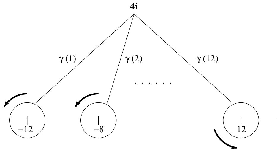
The fundamental group $\pi_{1}({\bf P}^{1}-{\rm Sing},\ast)$ acts on $H_{1}(E_{0},{\bf Z})$ as the monodromy group. We describe the generator system for it. Let $\gamma_{i}\enskip(i=1,\cdots,12)$ be a loop starting from $s_{0}$ and goes around $s_{i}$ in the positive sense on the upper half plain except the circuit around $s_{i}$ (see Fig.2 ).

By a direct observation we can calculate the monodromy transformation $T_{j}=T(\gamma_{j})$ of $H_{1}(E_{0},{\bf Z})$ along $\gamma_{j}$ with respect to the basis $\{\alpha_{1},\alpha_{2}\}$.

We choose a fixed point ${\underline{s}}$ in the lower half plane of ${\bf P}^{1}(s)$. Make cut lines $c_{i}$ by the line segment between ${\underline{s}}$ and $s_{i}\ \ (i=1,\cdots,12)$. By restricting $(S_{0},\pi_{1},{\bf P}^{1})$ on ${\bf P}^{1}-\cup_{i=1}^{12}c_{i}$ we have a topologically trivial fibration. So we can determine the cycles $\alpha_{1},\alpha_{2}$ of $H_{1}(\pi^{-1}(s),{\bf Z})$ for any $s\in{\bf P}^{1}-\cup_{i=1}^{12}c_{i}$ using this trivialization. If we make the continuation of the system $\{\alpha_{1},\alpha_{2}\}$ passing through the line $c_{i}$ from left to right, It is transformed according to Table 1.

Let $r$ be an oriented arc on ${\bf P}^{1}(s)$ starting from $s_{0}$. We make a 2-chain on $S_{0}$ by the continuation of a starting 1-cycle $\alpha\in H_{1}(E_{0},{\bf Z})$ along $r$, and denote it by

$$r\times\alpha.$$

Here we define its orientation as the ordered pair of the ones of $r$ and $\alpha$. Using this notation we make a system $\{\Gamma_{1},\cdots,\Gamma_{8}\}$ of 8 elements in $H_{2}(S_{0},{\bf Z})$ (see Fig.3, Fig.4, Fig.5, Fig.6):

	$\displaystyle\Gamma_{1}=\gamma(7)^{-1}\gamma(8)^{-1}\gamma(9)^{-1}\gamma(11)^{-1}\gamma(12)^{-1}\times\alpha_{1},$
	$\displaystyle\Gamma_{2}=\gamma(4)^{-1}\gamma(5)^{-1}\gamma(6)^{-1}\gamma(7)^{-1}\gamma(8)^{-1}\gamma(9)^{-1}\times\alpha_{2},$
	$\displaystyle\Gamma_{3}=\gamma(5)^{-1}\gamma(6)^{-1}\gamma(7)^{-1}\gamma(8)^{-1}\times\alpha_{1},$
	$\displaystyle\Gamma_{4}=\gamma(2)^{-1}\gamma(3)^{-1}\gamma(4)^{-1}\gamma(5)^{-1}\times\alpha_{2},$
	$\displaystyle\Gamma_{5}=\gamma(12)\times(\alpha_{1}+\alpha_{2})+\gamma(10)^{-1}\gamma(11)^{-1}\gamma(12)^{-1}\times(-\alpha_{2}),$
	$\displaystyle\Gamma_{6}=\gamma(6)\times(\alpha_{1}+\alpha_{2})+\gamma(4)^{-1}\gamma(5)^{-1}\gamma(6)^{-1}\times(-\alpha_{2}),$
	$\displaystyle\Gamma_{7}=\gamma(9)\times(\alpha_{1}-\alpha_{2})+\gamma(7)^{-1}\gamma(8)^{-1}\gamma(9)^{-1}\times(-\alpha_{1}),$
	$\displaystyle\Gamma_{8}=\gamma(3)\times(\alpha_{1}-\alpha_{2})+\gamma(1)^{-1}\gamma(2)^{-1}\gamma(3)^{-1}\times(-\alpha_{1}).$

where the composite arcs are performed from right to left.

We note that any of $\{\Gamma_{1},\cdots,\Gamma_{8}\}$ is a 2-cycle according to the monodromy action in Table 1. So we regard them a system in $H_{2}(S_{0},{\bf Z})$. Let $L(\Gamma)$ denote the sublattice $\oplus{\bf Z}\Gamma_{i}$.

Next we construct another system that is dual to $L(\Gamma)$. Let $r(i)$ be the oriented line segment from $s_{0}$ to $s_{i}$. Using this notation we construct 8 elements in $H_{2}(S_{0},{\bf Z})$ ( see Fig.7):

	$\displaystyle C_{1}=(r(6)-r(7))\times\alpha_{2},$
	$\displaystyle C_{2}=(r(9)-r(10))\times\alpha_{1},$
	$\displaystyle C_{3}=(r(7)-r(12))\times\alpha_{2},$
	$\displaystyle C_{4}=(r(4)-r(9))\times\alpha_{1},$
	$\displaystyle C_{5}=r(10)\times\alpha_{1}-r(11)\times(\alpha_{1}+\alpha_{2})-r(12)\times\alpha_{2},$
	$\displaystyle C_{6}=r(4)\times\alpha_{1}-r(5)\times(\alpha_{1}+\alpha_{2})-r(6)\times\alpha_{2},$
	$\displaystyle C_{7}=-r(7)\times\alpha_{2}-r(8)\times(\alpha_{1}-\alpha_{2})-r(9)\times\alpha_{1},$
	$\displaystyle C_{8}=-r(1)\times\alpha_{2}-r(2)\times(\alpha_{1}-\alpha_{2})-r(3)\times\alpha_{1}.$

We note that any element of $\{C_{1},\cdots,C_{8}\}$ ends with a vanishing cycle at the terminal point of the base arc. So it is a 2-cycle on $S_{0}$. Let $L(C)$ denote the sublattice $\oplus{\bf Z}C_{i}$.

[Proof]. We can calculate all the intersection numbers by a direct observation of the cycles. For example we consider $\Gamma_{1}\cdot\Gamma_{2}$. They have 2 intersections on a vertical line between $4$ and $\sqrt{19}$ of $\Gamma_{2}$ saying $p_{1},p_{2}$ (see Fig.8).

At the upper intersection $p_{1}$ the base arcs intersect with a negative sign, and the fibre cycles $\alpha_{1},\alpha_{2}$ intersect with a positive sign. By considering the definition of the orientation on $\Gamma_{i}$ we get there intersection number $+1$. The situation is quite the same for the intersection in the lower half plane. So we have $\Gamma_{1}\cdot\Gamma_{2}=2$. We can proceed this type of calculation until we get the full intersection matrices.

q.e.d.

Proof]. The first statement is a direct consequence of the fact that $(\Gamma_{i}\cdot C_{j})$ is a unimodular matrix.

Suppose $L(\Gamma)$ is not primitive. It means that there is an element $\lambda\in L-L(\Gamma)$ with $k\lambda\in L(\Gamma)$ for some integer $k$.Put

$$k\lambda=\sum_{i=1}^{8}k_{i}\Gamma_{i}.$$

Then we have

$$k(\lambda\cdot\check{\Gamma}_{i})=(k\lambda)\cdot\check{\Gamma}_{i}=k_{i}.$$

It indicates $k\mid k_{i}\ (i=1,\cdots,8)$. So it is deduced $\lambda\in L(\Gamma)$. This is a contradiction.

q.e.d

For the moment we study the divisors on the reference surface $S_{0}$. Let $P_{ij}^{\pm}$¡¡denote two intersections $H_{i}\cap H_{j}\ \ (1\leq i<j\leq 4)$, here we distinguish them by the signature of the $s$-coordinate ( see Proposition 1.1). The surface $S_{0}$ has an exceptional curve corresponding to every intersection $P_{ij}^{\pm}\ \ (1\leq i<j\leq 4)$. We denote them by $E_{ij}^{\pm}$. Let us consider the projection $\pi:S\rightarrow{\bf P}^{1}\times{\bf P}^{1}$. Let $F_{s}$ denote the pull back $\pi^{\ast}({\bf P}^{1}(s))\times\{t\})$ of the generic $s$-coordinate line, and let $F_{t}$ denote the pull back of the generic $t$-coordinate line. Set

$$G_{i}=\frac{1}{2}(\pi^{\ast}H_{i}-\sum_{j\not=i}(E_{ij}^{+}+E_{ij}^{-})),\ (i=1,2,3,4).$$

This is the reduced divisor coming from the 4 sections $H_{i}$ of the elliptic fibration $(S_{0},\pi_{1},{\bf P}^{1}(s))$.By an easy observation we have the following.

Proof]. Set the sublattices $L_{i}\ \ (i=1,2,3)$ as follows:

	$\displaystyle L_{1}=\langle G_{1},E_{14}^{+},E_{14}^{-},F_{t}-E_{23}^{+}\rangle,$
	$\displaystyle L_{2}=\langle G_{2},E_{24}^{+},E_{24}^{-},F_{t}-E_{13}^{+}\rangle,$
	$\displaystyle L_{3}=\langle G_{3},E_{34}^{+},E_{34}^{-},F_{t}-E_{12}^{+}\rangle.$

They are isometric with the lattice

$$D_{4}=\begin{pmatrix}-2&1&1&1\\ 1&-2&0&0\\ 1&0&-2&0\\ 1&0&0&-2\end{pmatrix},$$

and they are perpendicular each others. Set

	$\displaystyle\Delta_{1}=F_{s}+F_{t}-E_{12}^{+}-E_{13}^{+}-E_{23}^{+},$
	$\displaystyle\Delta_{2}=G_{1}+G_{2}+G_{3}-G_{4}+F_{s}+3F_{t}-E_{12}^{+}-E_{13}^{+}-E_{23}^{+},$

then we have

$$\Delta_{1}\cdot\Delta_{1}=-2,\Delta_{1}\cdot\Delta_{2}=0,\Delta_{2}\cdot\Delta_{2}=2.$$

Now we put

$$P=L_{1}\oplus L_{2}\oplus L_{3}\oplus\langle\Delta_{1}\rangle\oplus\langle\Delta_{2}\rangle.$$

Then it holds

	$\displaystyle P\subset L(div)\subset L(\Gamma)^{\perp},$
	$\displaystyle{\rm rank}\ P=14,{\rm discr}\ P=-2^{8}.$

On the other hand we have ${\rm discr}\ L(\Gamma)=2^{8}$. By considering the fact that $L$ is unimodular and $L(\Gamma)$ is a primitive sublattice, we get the conclusion that $P=L(div)=L(\Gamma)^{\perp}$.

q.e.d.

Now we extend Proposition 1.4 to the general situation.

[Proof]. We note that the family ${\cal F}=\{S(x)\}$ is fibred over the parameter space of ${\rm M}(2,{\bf C})^{4}$ . This fibration is locally topological trivial on a Zariski open subset in $X^{\circ}\subset{\rm M}(2,{\bf C})^{4}$. Using this trivialization we can proceed the same argument for a general member as for the specialized element $S_{0}$.In fact always $L(div)$ and $P$ are defined as a sublattice in ${\rm Pic}(S(x))$. We have the systems $L(\Gamma)$ and $L(C)$ also. So Proposition 1.4 is valid for every $S$ of $\mathcal{F}$. If the condition is satisfied, then $L(\Gamma)$ cannot contain any divisor class. Hence we obtain the required conclusion.

q.e.d

In this section we show the converse of Theorem 1. Before starting this argument we state some general properties of a $K3$ surface.

This is deduced from the Riemann-Roch theorem by a routine argument.

Let us consider the lattice

$\displaystyle P={D}_{4}^{3}\oplus\langle-2\rangle\oplus\langle 2\rangle,$

(2.1)

and we let $(\ast,\ast)$ denote the bilinear form on an abstract lattice $P$.

By the argument in Section 1 we can find the generator system of $P$:

$\displaystyle f_{s},\quad f_{t},\quad g_{i}\ \ (i=1,\cdots,4),\quad e_{ij}^{+},\ \ e_{ij}^{-}\ \ (i\neq j,1\leq i,j\leq 4),$

(2.2)

with the following properties among them :

(p1)

	$\displaystyle(g_{i},g_{i})=-2,\quad(f_{s},f_{t})=2,\quad(g_{i},f_{s})=(g_{i},f_{t})=1$
	$\displaystyle(g_{i},e_{ij}^{+})=(g_{i},e_{ij}^{-})=1,\quad(e_{ij}^{+},e_{ij}^{+})=(e_{ij}^{-},e_{ij}^{-})=-2,$

and all other intersections equal $0$,

(p2)

$\displaystyle f_{s}+f_{t}=2g_{i}+\sum_{j\neq i}(e_{ij}^{+}+e_{ij}^{-}).$

We note that this system is determined uniquely up to isometries of $P$.

[Proof]. Always we regard the element of $P$ under the identification in ${\rm(a)}$ or ${\rm(a^{\prime})}$. We show the first assertion.

(Claim 1)  We can assume that every $e_{ij}^{\pm}$ is effective.

Let $e$ be one of the twelve elments $e_{ij}^{\pm}$. Since $e\cdot e=-2$, either $e$ or $-e$ is effective. If $-e$ is effective then we perform the reflection $\gamma$ on ${\rm Pic}(S)$ determined by $e$. And we can use

$$\gamma(f_{s}),\quad\gamma(f_{t}),\quad\gamma(g_{i}),\quad\gamma(e_{ij}^{\pm})$$

instead of the system $(2.2)$. According to the orthogonality of the system $\{e_{ij}^{\pm}\}$ we can iterate this procedure until we get the required effective system. Since we have $\gamma(f_{s})=f_{s},\gamma(f_{t})=f_{t}$, the nef property for $f_{s},f_{t}$ is always satisfied throughout this process.

References

• [1] W. Barth, C. Peter and A. van de Ven, Compact complex surfaces, Springer(1984).
• [2] E. Freitag and C. F. Hermann, Some modular varieties of low dimension, preprint.
• [3] K. Kodaira, On analylic surfaces II, Ann. Math., 77(1963), 563 - 626.
• [4] K. Koike, The Kuga - Satake variety attached to the double covering of 𝐏1×𝐏1{\bf P}^{1}\times{\bf P}^{1} branched along four curves of bidegree (1,1)(1,1), preprint.
• [5] M. Kitazume, K. Koike, and H. Shiga, Notes on a certain integral orthogonal group and its quotient by the principal congruence subgroup of level 2, to be appeared in Kyushu J. Math. .
• [6] K. Matsumoto, Theta functions on the bounded symmetric domain of type I2,2I_{2,2} and the period map of a 4 - parameter family of K3 surfaces, Math. Ann., 295(1993), 383 - 409.
• [7] K. Matsumoto and T. Sasaki, On the system of differential equations associated with a quadric and hyperplanes, Kyushu J. Math., 50(1996), 93 - 131.
• [8] K. Matsumoto, T. Sasaki and M. Yoshida, The monodromy of the period map of a 4 - parameter family of K3 surfaces and the hypergeometric function of type (3,6), Int. J. Math., 3(1992), 1 - 164.
• [9] K. Matsumoto and M. Yoshida, Certain reflection groups acting on symmetric domains of type IV, Mem. Fac. Sci. Kyushu Univ., Ser. A, vol. 46(1992), 115 - 128.
• [10] V. V. Nikulin, Integral symmetric bilinear forms and some of their applications, Math. USSR Izv., 14(1980), 103 - 166.
• [11] K. Paranjape, Abelian varieties associated to certain K3 surfaces, Compositio Math., 68(1988), 11 - 22.
• [12] I. I. Pjateckiĭ - Šapiro and Šafarevič, A Torelli theorem for algebraic surfaces of type K3, Math. USSR Izv., 5(1971), No.3, 547 - 588.
• [13] I. Satake, Clifford algebras and families of Abelian varieties, Nagoya Math.J. 27(1966), 435-466.
• [14] M. Saito, B. Sturmfels and N. Takayama, Gröbner Deformations of Hypergeometric Differential Equations. Algorithms and Computation in Mathematics, Vol. 6, Springer(1999).
• [15] H. Shiga, On the arithmetic properties of the modular function induced from the hypergeometric differential equation of type (3,6)(3,6), Proc. 7th Int. Coll. Differential Equations Provdiv 1996, 381 - 388.
• [16] B. van Geemen, Kuga - Satake varieties and the Hodge conjecture, To appear in Proc. NATO ASI and CRM Summer School Banff 1998.
T. Tsutsui
Department of Mathematics and Informatics
Faculty of Science
Chiba University
Yayoi-cho Inage-ku Chiba 263-8522, JAPAN
K. Koike, H. Shiga
Graduate School of Science
N. Takayama
Department of Mathematics
Kobe University
Rokko Kobe 657-8501, JAPAN