Limiting distributions for a polynuclear growth model
with external sources

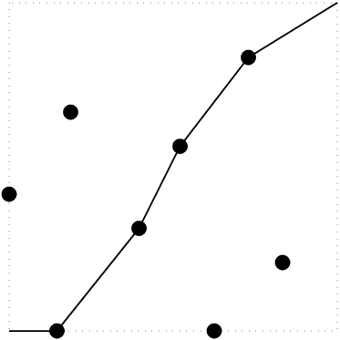
Our main object of study is the following combinatorial problem. Fix three real parameters $t>0$ and $\alpha_{\pm}\geq 0$. We construct a random set of points in the unit square $[0,1]\times[0,1]\subset\mathbb{R}^{2}$, as follows. Let $P(\lambda)$ denote a Poisson variable of density $\lambda$. We select $P(t^{2})$ points at random inside the square $(0,1)\times(0,1)$, $P(\alpha_{+}t)$ points at random on the open bottom edge $(0,1)\times\{0\}$, and $P(\alpha_{-}t)$ points at random on the open left edge $\{0\}\times(0,1)$. Hence no point is selected from the lower left vertex and from the closed top and right edges. For example, in Figure 1, 5 points are selected inside the square, and 2 and 1 points in the bottom and the left edges, respectively. A (weakly) up/right path is given by a sequence of points such that each point is (weakly) above and to the right of its predecessor; thus the solid line in the figure is a (weakly) up/right path from the lower left vertex to the upper right vertex.

The length of a (weakly) up/right path is defined by the number of points in the path; thus the up/right path of the example has length $4$.

We define $L(t)$ be the length of the longest (weakly) up/right path in this random configuration of points. (This, of course, implicitly depends on the values of $\alpha_{\pm}$.) E.g., the solid line in Figure 1 is the longest up/right path of the example. In general, there may be more than one longest path, but we are only interested in the length $L(t)$, hence the degeneracy is not an issue. We note that the above process can be thought of in an alternative way as a Poisson process of intensity $1$ in the open $\mathbb{R}_{+}^{2}$, together with a Poisson process of intensity $\alpha_{+}$ on the open half-line $\mathbb{R}_{+}\times\{0\}$ and a Poisson process of intensity $\alpha_{-}$ on the open half-line $\{0\}\times\mathbb{R}_{-}$. Then $L(t)$ is equal to the length of the longest (weakly) up/right path from $(0,0)$ to $(t,t)$.

The main interest in this paper is the statistics of $L(t)$ as $t\to\infty$, as this problem arose in a polynuclear growth (PNG) model considered by Prähofer and Spohn in [13]. PNG is a simplified model for layer by layer growth in one spatial dimension. At each random nucleation position, an island of height 1 is formed and spreads laterally with speed 1. When two islands meet, they form one island and keep spreading with the same speed. The question is the fluctuations of the height in the large time limit.

As a special case, suppose that a single island starts spreading at the origin and that further nucleation takes place only on top of this ground layer. Furthermore, suppose that there are external nucleation sources at the two ends of the ground layer. Then the height, for example, at the origin at time $\sqrt{2}t$ is equal to $L(t)$ in the above point selection process. We refer the interested readers to the papers [13, 12] for details of the mapping from PNG to $L(t)$ and many other related works.

In the above point selection process, a special case is when $\alpha_{\pm}=0$ : $P(t^{2})$ points are selected inside the square with no points on the edges. (This corresponds to a PNG model without external nucleation sources.) It is interesting that in this case, there is a combinatorial interpretation. Consider a random permutation of $S_{N}$. If we take $N$ as Poisson variable $P(t^{2})$, the longest increasing subsequence of a random permutation of $S_{N}$ has the same statistics as $L(t)$ (see [2] and references therein). The limiting fluctuation of $L(t)$ in this case is obtained in [2] : there is a distribution function $\FGUE(x)$ such that

The convergences of all the moments are also proved in the same paper. Here $\FGUE$ is the so-called GUE Tracy-Widom distribution function of random matrix theory. See Section 2 for the explicit formula of $\FGUE$, equation (2.9).

The “GUE” in $\FGUE$ refers to the Gaussian unitary ensemble, the set of all $N\times N$ Hermitian matrices together with the probability measure defined by

where $Z_{N}$ is a normalization constant (see e.g. [10, 5]). Tracy and Widom in [14] proved that as $N\to\infty$, the properly centered and scaled largest eigenvalue of a random GUE matrix converges in distribution to $\FGUE$. Therefore the above result (1.1) implies that in the limit, $L(t)$ with $\alpha_{\pm}=0$ and the largest eigenvalue of a random GUE matrix have the same fluctuations.

In this paper, we obtain similar limiting distributions in the presence of points on the edges. When $\alpha_{\pm}>0$, the longest path begins by following one of the edges for a while, then enters the square. Hence when $\alpha_{\pm}$ are small, the effect coming from edges is small, and we expect $L(t)$ to have the same statistics as when $\alpha_{\pm}=0$, i.e. GUE fluctuation. But when $\alpha_{\pm}$ is large, the longest path lies mostly on one of the edges, hence we expect Gaussian fluctuation. It turns out that the critical case is when $\alpha_{\pm}=1$. We need to distinguish four different cases to state the results. In each case, $\alpha_{\pm}$ are fixed.

• •

  When $\alpha_{\pm}<1$, we obtain $\FGUE$ in the limit.

• •

  When either of $\alpha_{\pm}$ is greater than $1$, we obtain Gaussian fluctuation.

• •

  When one of $\alpha_{\pm}$ is equal to $1$ and the other is strictly less than $1$, we obtain $\FGOE(x)^{2}$. In the above definition of the GUE, if we replace Hermitian matrices by real symmetric matrices, we obtain the Gaussian orthogonal ensemble (GOE). The limiting distribution of the (properly centered and scaled) largest eigenvalue of a random GOE matrix is given by $\FGOE$ in [15] (see Section 2 for the explicit formula). The above limit $\FGOE(x)^{2}$ can be interpreted as follows : take two random GOE matrices and superimpose their eigenvalues. The largest of the superimposition of eigenvalues has limiting fluctuation $\FGOE^{2}$.

• •

  When $\alpha_{\pm}=1$, we have a new limiting distribution which we denote $\F 0$, for which we do not yet have a random matrix interpretation. See Section 2 for the definition and discussions.

More explicitly, we have the following theorem.

The functions, $\FGUE$, $\FGOE$ and $\F 0$, in the above theorem are defined in Section 2, and we discuss their properties in the same section.

The above theorem shows that there are certain transitions around the points $\alpha_{\pm}=1$. It is of interest to investigate these transitions in detail. In Section 3, under proper scalings of $\alpha_{\pm}\to 1$, we obtain new classes of distribution functions interpolating the functions of the above theorem.

In addition to the above point selection process, there is a closely related lattice directed polymer model in 2-dimensional space, which is a generalization of the model considered by Johansson in [9]. This model and a related exclusion process are discussed in Section 4.

Finally the proofs of the theorems are discussed in Section 5.

Let $u(x)$ be the solution to the Painlevé II (PII) equation,

with the boundary condition

where $Ai$ is the Airy function. The proofs of the (global) existence and the uniqueness of the solution were established in [8]. The asymptotics as $x\to-\infty$ are given by (see e.g. [8, 7])

Recall that $Ai(x)\sim\frac{e^{-(2/3)x^{3/2}}}{2\sqrt{\pi}x^{1/4}}$ as $x\to+\infty$. Define

so that $v^{\prime}(x)=(u(x))^{2}$. We note another expression

which can be obtained by noting that the difference (i) has derivatives equal to zero by the PII equation, and (ii) becomes zero as $x\to\infty$ by (2.3).

The Tracy-Widom distribution functions are defined in terms of $u$ and $v$.

It is proved by Tracy and Widom in [14, 15] that under proper centering and scaling, the distribution of the largest eigenvalue of a random GUE/GOE/GSE matrix converges to $\FGUE(x)$ / $\FGOE(x)$ / $\FGSE(x)$ as the size of the matrix becomes large. The readers are referred to [10, 5] for definitions of various random matrix ensembles and their basic properties. We note that from the asymptotics (2.3) and (2.4), for some positive constant $c$,

Hence in particular, as $x\to+\infty$, all the above three functions become $1$, and as $x\to-\infty$, they become $0$. Monotonicity follows from the fact that they are limits of sequences of distribution functions, and therefore (2.9)-(2.11) are indeed distribution functions.

We need a new distribution function for the case when $\alpha_{\pm}=1$ in Theorem 1.1.

The asymptotics (2.3)-(2.5) imply that $\F 0(x)$ has limit $1$ as $x\to+\infty$ and $0$ as $x\to-\infty$. The monotonicity of $\F 0$ follows from the fact that it is a limit of distribution functions in Theorem 1.1. It would of interest to have random matrix interpretation of the function $\F 0$, but so far we have been unable to identity $\F 0$ as a quantity arising in random matrix theory.

One special property of this distribution function is that it has mean zero.

In this section, we investigate the transition around $\alpha_{\pm}=1$ in detail.

To state the results, Theorem 3.3, we need some preliminary definitions. Let $\Gamma$ be the real line $\mathbb{R}$, oriented from $+\infty$ to $-\infty$. Let $m(\cdot;x)$ be the solution to the Painlevé II Riemann-Hilbert problem :

Here $m_{+}(z;x)$ (resp., $m_{-}$) is the limit of $m(z^{\prime};x)$ as $z^{\prime}\to z$ from the left (resp., right) of the contour $\Gamma$ : $m_{\pm}(z;x)=\lim_{\epsilon\downarrow 0}m(z\mp i\epsilon;x)$. The relation between the above Riemann-Hilbert problem and the Painlevé II equation is the following (see, e.g., [7]). If we expand

we have

where $u(x)$ and $v(x)$ are defined in (2.1)-(2.5). The above Riemann-Hilbert problem is the special case of monodromy data $p=-q=1$, $r=0$ in the standard family of Painlevé II Riemann-Hilbert problems.

Define

From the jump condition of the Riemann-Hilbert problem (3.1), $a(x,w)$ and $b(x,w)$ are continuous at $w=0$. Indeed since $m_{-}v$ in the upper half plane of $\mathbb{C}$ is an analytic continuation of $m_{+}$ in the lower half plane of $\mathbb{C}$, $a(x,w)$ and $b(x,w)$ are analytic in $w$. We have the following properties of $a,b$.

We now define the following functions with parameters $w_{+},w_{-},w$.

From Lemma 3.1 (ii), $H$ and $G$ have the limit $1$ as $x\to\infty$ and has the limit $0$ as $x\to-\infty$ for each fixed $w_{+},w_{-},w$. Also theorem 3.3 below shows that they are limits of distribution functions. Therefore $H$ and $G$ are distribution functions. These distribution functions interpolate between the functions $\FGUE$, $\FGOE^{2}$ and $\F 0$ of theorem 1.1. The following results follow from Lemma 3.1 (iii), (vi).

Now the main theorem in this section is that if we take proper scaling of $\alpha_{\pm}\to 1$ in $t$, we obtain the above functions in the limit.

A special case of (ii) is when $w_{+}=-w_{-}$, which corresponds to $\alpha_{+}\alpha_{-}=1$. In this case, the limiting shape of PNG has curvature $0$ (see [13]). Hence we obtain a one-parameter family of distribution functions for fluctuations of a flat curvature PNG. We have the exact values of the means which include Proposition 2.1 as a special case when $w=0$.

In this section, we analyze a certain lattice directed polymer problem which is closely related to the point selection model discussed above.

Let $\mathbb{N}=\{1,2,3,\cdots\}$ and $\mathbb{N}^{*}=\{0,1,2,\cdots\}$. Let $0<q<1$, $\alpha_{\pm}\geq 0$ be fixed numbers such that $\alpha_{\pm}\sqrt{q}<1$. We denote by $g(q)$ the geometric distribution with parameter $q$ :