Gauß Cubature for the Surface of the Unit Sphere
Abstract
Gauß cubature (multidimensional numerical integration) rules are the natural generalisation of the 1D Gauß rules. They are optimal in the sense that they exactly integrate polynomials of as high a degree as possible for a particular number of points (function evaluations). For smooth integrands, they are accurate, computationally efficient formulae.
The construction of the points and weights of a Gauß rule requires the solution of a system of moment equations. In 1D, this system can be converted to a linear system, and a unique solution is obtained, for which the points lie within the region of integration, and the weights are all positive. These properties help ensure numerical stability, and we describe the rules as ‘good’. In the multidimensional case, the moment equations are nonlinear algebraic equations, and a solution is not guaranteed to even exist, let alone be good. The size and degree of the system grow with the degree of the desired cubature rule. Analytic solution generally becomes impossible as the degree of the polynomial equations to be solved goes beyond , and numerical approximations are required. The uncertainty of the existence of solutions, coupled with the size and degree of the system makes the problem daunting for numerical methods.
The construction of Gauß rules for (fully symmetric) -dimensional regions is easily specialised to the case of , the unit sphere in 3D. Despite the problems described above, for degrees up to , good Gauß rules for have been constructed/discovered.
1 Introduction
1.1 Multidimensional Gauß Cubature
Instead of directly considering the surface of the unit sphere , we will consider a more general case. For -dimensional regions , we will construct -point cubature rules of the form:
The are called the cubature points, and the are their respective weights. We want rules that are as accurate as possible for a given number of points (function evaluations). Smooth integrands may be accurately approximated by polynomials, hence Gauß rules, which exactly integrate all polynomials of as high a degree as possible, are a natural choice. For numerical stability, we also want rules with positive weights, and points which lie within (these things are automatic in 1D). Up until about 1975, the best rules known were the (Cartesian) product rules, which although good, are not optimal.
The theory behind multidimensional Gauß rules for ‘fully symmetric’ is a natural generalisation of the well-known 1D case. It originates in a foundation paper by Mantel and Rabinowitz (1977) [18]. The material has been applied to the case of [9], although no computed rules have been published.
We describe, in §2, the theory behind the construction of Gauß cubature rules for fully symmetric regions . The material is specialised to the case of in §3, which describes implementational details and some computer programs. For degrees up to , good cubature rules for have been found, and these are listed in Appendix B. By comparison, the (non-optimal) product rules for are simple to construct, and are not terribly inefficient. We describe them, and some programs for their computation, in §4. Alternative methods for cubature, such as Monte Carlo and lattice methods are discussed in §4.4. In general they are poor second choices when Gauß rules are available.
Before progressing, we sketch an application of the use of cubature for : the solution of the interior Dirichlet problem using a boundary integral equation. More significant applications are from statistics, where cubatures over many dimensions are required, and efficiency is critical.
1.2 Application: 3D Interior Dirichlet Problem
Definition 1.1 (3D Interior Dirichlet Problem)
Given a smooth, bounded domain , with boundary , find such that:
- 1.
satisfies Laplace’s equation within , that is , .
- 2.
is known on the boundary (the Dirichlet condition). That is, there is a continuous function such that: , .
We will consider only domains of class [12, pp 21-22], which we will loosely call ‘smooth’. (Their boundaries will be of class .) By , we mean the set of times continuously differentiable real-valued functions defined on . We will be interested in functions contained in .
The interior Dirichlet problem is a convenient model problem to work with. Its solution represents a potential function, that is readily related to physical observables (e.g. electrostatic force). It is mathematically attractive, as the existence of a unique solution is known. Where the boundary , and the boundary data are simple, it may even be possible to find an analytic solution. In general, however, this is not possible, and it is more sensible to construct a numerical approximation. Knowledge of the existence of a unique solution, for even quite nonsmooth boundaries, greatly encourages this. Techniques to (approximately) solve the interior Dirichlet problem may be able to be used as models for the solution of more sophisticated boundary value PDEs.
One method of solving the interior Dirichlet problem is to reformulate it in terms of a boundary integral equation on . This reformulation is a natural choice: it is involved in a constructive proof of the existence of a solution [12]. We begin by defining the ‘fundamental solution of Laplace’s equation in 3D’ as the function:11 1 A different function is defined for a different number of dimensions, notably .
For fixed , is harmonic (satisfies Laplace’s equation) in . Writing as the unit outward normal of at the point , we construct the solution to the interior Dirichlet problem in terms of the fundamental solution as follows:
Theorem 1.1 (Solution to the interior Dirichlet problem)
For , the double layer potential
with continuous density is a solution of the interior Dirichlet problem if is the solution of the following integral equation, for :
A numerical approximation to the solution of the BIE can be used to construct a numerical approximation to the double layer potential , and hence the solution to the Dirichlet problem [1]. Initially, we construct a cubature rule for approximating integrals over . This cubature rule is used with a Galerkin technique to approximate the solution of the BIE for . Lastly, is approximated within by application of the cubature rule to the Galerkin approximation. A cubature rule for the manifold may be constructed by pointwise projection from one for . An advantage of this is that for a particular number of desired points in the rule, a single rule for will suffice for any manifold. A disadvantage is that although the rule may be appropriate for , the mapping process may reduce its efficacy. An even point density on may lose its regularity when mapped, especially if is not concave. To illustrate this, [2] uses the following region in experiments:
A typical choice is . As decreases towards , the shape becomes less convex, eventually becoming like a peanut, and numerical methods lose accuracy.
2 Gauß Cubature for Fully Symmetric Regions
2.1 Motivation for Cubature
Let be an -dimensional region contained in ; and . Consider the numerical approximation of multiple integrals of the form:
Here, is a weighting function, typically defined to contain the ‘singularity’ of the integrand. For example if is , a typical weighting function is , and for a wide class of functions (e.g. polynomials), the integral will exist. Commonly will be unity, and will be spherically symmetric about the origin. For example, if is , we might have:
Accurate approximation of multidimensional integrals is in general a computationally expensive task. The rapid growth in expense with has been called the ‘curse of dimensionality’ (see §4.1). Fortunately, for many applications, has some symmetry (consider ), and this can greatly simplify both the construction and the application of rules. Here, we consider the case where has some symmetry (not an issue in 1D!), and the construction of Gauß rules, which minimise computational expense for a desired accuracy. The philosophy is that if and have a certain symmetry, then it will be natural to place equally-weighted cubature points within according to the same symmetry. This symmetry should considerably reduce the computations required to construct the rule.
2.2 Full Symmetry
One of the most natural symmetries to conceive for is full symmetry in Cartesian coordinates. A set of points is fully symmetric if any point can be reached from any other point by a series of orthogonal rotations about coordinate axes, and reflections in coordinate planes. Observe that in 3D, the set of vertices of the unit octahedron is fully symmetric; indeed a complete fully symmetric set of points is an orbit under the action of the group of symmetries of the octahedron. This group has order , and includes both rotations and reflections. In particular is composed of complete sets of fully symmetric points.
The use of symmetry for cubature rules dates back to Russian works in the 1960s, primarily in papers by Sobolev [24, 25, 23]. Other symmetries for 3D can be defined in terms of the symmetry groups of other Platonic solids. The immediately attractive case is that of the dodecahedron/icosahedron, but this is harder to visualise than that of the octahedron (where the vertices all lie on the coordinate axes), and leads to more difficult algebra to disentangle. In any case, alternative symmetries have little application beyond 3D, whilst the notion of full symmetry generalises perfectly. The notion of full symmetry dates back to Lyness (1965) [15], and the use of octahedral symmetry for cubature on was first put on a clear foundation by Lebedev (1976) [14]. Shortly after this, the foundation paper of Mantel and Rabinowitz (1977) [18] generalised the notion to arbitrary fully symmetric domains, implicitly using the octahedral symmetry, although not acknowledging the intellectual heritage. This presentation of the theory closely follows both [18] and a complementary paper by Keast and Lyness (1979) [11]. To begin, we formalise the notion of full symmetry.
Definition 2.1 (Full Symmetry between Two Points)
and are a pair of fully symmetric (FS) points in , denoted , if can be reached from by permutations and/or sign changes of the entries of .
Observe that “” is an equivalence relation, and thus it induces a partition of into equivalence classes. Suppose that point has non-zero coordinates, of which are distinct, and let the th distinct non-zero coordinate appear times (), so that . Trivially, . For this , a point can then be found such that:
| (2) |
Here we have chosen . This is called the generator of the equivalence class, and each class can be expressed uniquely in terms of a generator. The number of distinct points in the equivalence class containing generator can be shown to be:
The number of elements in each class thus varies between (for the equivalence class ) and (in general). The exact number will be important for our work.
Definition 2.2 (Full Symmetry for a Set of Points)
A set of points is called fully symmetric (FS) if and imply , that is the set contains only complete equivalence classes.
Clearly is an FS set of points. Other important examples of
FS sets of points (domains of integration) commonly found in the
literature are the -dimensional unit hypercube
; the -dimensional unit sphere
;
and its surface . In §3, we will be interested
in .
Definition 2.3 (Full Symmetry for a Function)
Given an FS domain , a function is said to be a fully symmetric (FS) function if: for all , means that .
It is not really necessary that the function be real-valued for this definition to make sense, but this will be sufficient. We will only consider integrals over FS regions involving FS weight functions, and will be approximating them using cubature rules on FS sets of points. Where is an -dimensional FS region, consider an integrand , which is not necessarily fully symmetric, and an FS weight function which is positive over a set of positive volume:
This is to be approximated by an -point cubature rule , such that and , for . The rule is then:
| (3) |
Recall that the degree of a polynomial in variables is the maximum sum of the exponents in any of its terms, not the maximum exponent of any one variable appearing in its terms. Thus is a polynomial in (or more!) variables, that is of degree (not ), whilst and are monomials of degree . The rule is exact for a function , if . If it is exact for all polynomials in variables of degree up to and including , then it is called an integration rule of degree (of exactness) . Cubature rules of high degrees of exactness should accurately integrate smooth functions (which can be accurately approximated by polynomials), but this does not necessarily carry over to non-smooth functions.
Definition 2.4 (Fully Symmetric Integration Rule)
A cubature rule is
called a fully symmetric integration rule if the evaluation
points form an FS set, and all points in an FS equivalence class
within the rule have the same weight.
Note that this does not require to be FS, only that the set of evaluation points are an FS set (and that the weights are constant over all members of the same equivalence class). An FS integration rule is then completely specified by a set of generators and their corresponding weights. This can greatly simplify computations by reducing the number of points in a rule. The degree of an FS integration rule can be related to properties of polynomial integrands :
- 1.
If is a monomial containing an odd power of some coordinate variable, then .
- 2.
If is a monomial containing only even powers of variables, then and depend only on the exponents and not on the ordering of the variables.
Thus, an FS integration rule which is exact for all monomials of degree up to and including is actually a rule of degree , and it suffices that it be exact for all monomials of the form:
where and for and . (Set the monomial to if .)
This rule can be written, for an appropriate set of generators , with elements , each of which has an equivalence class with elements :
| (4) |
That is, to evaluate :
- 1.
For each equivalence class , sum the function values over all elements of the class.
- 2.
Multiply the weight associated with each generator by its respective equivalence class sum, and sum these multiples.
2.3 Gauß Cubature for Fully Symmetric Regions
Cubature rules that have a minimal number of points for a specified degree are called ‘minimal rules’.
Definition 2.5 (Fully Symmetric Minimal Rule)
An -point FS rule of degree over an FS set is a fully symmetric minimal (FSM) rule if no other FS rule of degree over exists with less than evaluation points.
Note that an FSM rule is not necessarily unique. In 1D, FSM rules are the unique Gauß rules, for which the theory is well-known. We must be careful not to confuse Gauß rules with product rules (see §4), where Gauß-Legendre rules are used as basic rules in the construction of (Cartesian) product multidimensional cubature rules. Sometimes these rules are called Gauß product rules. Whilst they are Gauß rules, in the sense that they exactly integrate polynomials of as high a degree as possible (but only in one dimension), they are not minimal. We would like our rule to possess a couple of important properties:
Definition 2.6 (Good Rule)
An integration rule over is a good rule if its evaluation points lie within , and its weights are positive.
The first of these conditions is familiar from 1D Gauß quadrature, whilst the second is new. These properties seem natural, however there is nothing in the assumptions for cubature that demands them. In 1D, naïve approaches to quadrature, such as the (equally-spaced) Newton-Cotes family, do not preserve the positivity of weights for larger , whilst both these properties are satisfied by 1D Gauß rules. In higher dimensions, Gauß rules are not necessarily good. The properties of good rules, in particular the latter, assist numerical stability. Whilst a rule may theoretically exactly integrate the relevant polynomials, in practice, summation of large terms of alternating sign tends to reduce numerical precision. In §3, we consider the case where is , so the internal points condition will simply require points to lie on the surface of the unit sphere.
We use the concept of full symmetry to define several classes of rules for the cubature of integrals with FS weight functions where the moments22 2 That is, the integrals of appropriate polynomials over . exist (commonly ). A fully symmetric cubature rule of degree exactly integrates all polynomials of degree up to and including . A fully symmetric minimal (FSM) rule does so using a minimal number of cubature points. A fully symmetric good (FSG) rule does so where all weights are positive and all points lie within . A fully symmetric minimal good (FSMG) rule is both minimal and good. A fully symmetric good minimal (FSGM) rule is a good rule that is minimal, that is, although FS rules on fewer points may exist, none are good.
We seek firstly FSMG rules, and if there are none of these, FSGM rules, which always exist. At worst, FSGM rules are product rules (see §4), which (generally) require points to be of degree . For low-dimensional applications (small ), this may not be terribly inefficient, e.g. product rules for actually require points. Apart from such considerations, a rule that is minimal (or almost so) might be almost good in the sense that negative weights are very small, or that points are only just outside , or that failing these conditions, errors in integrating polynomials are minor. The quest for good rules may be an arduous search through these almost good rules.
2.4 Conditions for Gauß Cubature in 3D
The procedure for constructing Gauß rules becomes more complicated as the dimension increases. Here, we fully develop the 3D case, specialising this to the case of in §3. We will set up a system of (moment) equations to express the fact that an FS rule for will exactly integrate all polynomials of up to a specified degree, without presupposing the number or distribution (beyond being an FS set) of points, or the sign of weights.
To begin, we group generators into types, depending on the number of zeros and repeated elements in the entries of their equivalence classes. There will always be the (not very interesting) class , of unit multiplicity, and in general other types of classes, for a total of types of classes. For small , this is generally small, and may be found as the solution to the following problem:33 3 The framing of this problem is the basis for the higher-dimensional analysis in [11].
Given a positive integer , is the total number of strings of length up to , with distinct entries taken from the positive integers , of the form:
such that and .
Answers to this problem can be found by counting the strings, and this is implemented in C as findec.c (Appendix C). Output from this program (for ) is presented in Appendix A. Not surprisingly, grows rapidly with . (This is just for curiosity purposes; will only apply the case .)
For the case , there are types of classes of points, listed in Table 1. There could be a generator at the origin, so that’s one type, called type . Generators on a coordinate axis are of a second type, called type , in which there are members of each equivalence class. Generators of the form , in a class of size , are of type , etc.44 4 Each of these generator types can be thought of in terms of geometrical arrangements of points on the surface of a unit sphere, projected from the vertices, edges and faces of the unit octahedron [14]. More generally, the generator in (2) is of type , and the complete set of types of generators in 3D is included in Table 1. This notation (from [8]), is simplified for the case in [18], where there are generators of each type, for , and we shall use the latter notation. We shall refer to our rule as having structure (an ordered set), usually just written .
| Class | Class | Number of Generators | Class | |||
|---|---|---|---|---|---|---|
| Number | Type | ([8] and [18]) | Names of Generators and Weights | Size | ||
| , | if | |||||
| , | ||||||
| , | ||||||
| , | ||||||
| , | ||||||
| , | ||||||
| , | ||||||
Given a structure , there will be a total of points in our rule, given by:
| (5) |
To construct Gauß rules, we proceed without presupposing the structure, instead attempting to find a structure such that the conditions for Gauß cubature are satisfied, and is minimised. Taking (such that the desired degree is ), and a rule structure , we write down a system of (moment) equations involving an appropriate set of generators, based on the requirement that a Gauß rule exactly integrates all -variable polynomials of each degree up to . It is in fact a sufficient requirement that we integrate exactly (-variable) monomials of these degrees. The system of moment equations is a system of nonlinear algebraic equations. (This is also true in 1D, although clever artifice allows us to reduce its solution to that of a linear system.)
For FS , the variables are listed in Table 1, and the system (4) expands to that presented in Figure 1. We will call this system , in accordance with [18, pp 410-411], where it first appears explicitly. System splits naturally into three subsystems, defined by the number of non-zero indices in the monomial that we wish to integrate exactly. Recall that the are non-negative integers, and the other variables are real. Also, although , we include it in a sum for consistency, and apply the convention that if . If , subsystem III is ignored, and if , subsystem II is also ignored.
Subsystem I: Subsystem II: Subsystem III:
Row-wise examination of the variables in Table 1 shows that, given , there are a total of:
variables in . To determine the number of equations, let be a positive integer and, for , let be the number of solutions in positive integers of:
For , we say there’s one solution if , and none otherwise. is the dimension of the space spanned by:
This can be efficiently computed by:
For each , there are equations in subsystem I, in II and in III. Hence, for a rule of degree , the total number of equations involved is . For , these numbers are listed in Table 2.
| 1 | 1 | 1 | 0 | 0 | 2 |
|---|---|---|---|---|---|
| 2 | 0 | 1 | 1 | 0 | 4 |
| 3 | 0 | 1 | 1 | 1 | 7 |
| 4 | 0 | 1 | 2 | 1 | 11 |
| 5 | 0 | 1 | 2 | 2 | 16 |
| 6 | 0 | 1 | 3 | 3 | 23 |
| 7 | 0 | 1 | 3 | 4 | 31 |
| 8 | 0 | 1 | 4 | 5 | 41 |
| 9 | 0 | 1 | 4 | 7 | 53 |
| 10 | 0 | 1 | 5 | 8 | 67 |
| 11 | 0 | 1 | 5 | 10 | 83 |
| 12 | 0 | 1 | 6 | 12 | 102 |
| 13 | 0 | 1 | 6 | 14 | 123 |
| 14 | 0 | 1 | 7 | 16 | 147 |
| 15 | 0 | 1 | 7 | 19 | 174 |
| 16 | 0 | 1 | 8 | 21 | 204 |
| 17 | 0 | 1 | 8 | 24 | 237 |
| 18 | 0 | 1 | 9 | 27 | 274 |
| 19 | 0 | 1 | 9 | 30 | 314 |
| 20 | 0 | 1 | 10 | 33 | 358 |
In general, may not have a unique solution, and indeed, may have no solutions. The best analytic technique currently available for the solution of systems of multivariable polynomial equations is the use of Groebner bases, see for example [5]. (The computer algebra package Mathematica uses this method.) Symbolic computations are expensive, however, and will fail to yield answers for polynomial equations of degree greater than . We are quickly led to numerical techniques! Fortunately, experience with shows that solutions commonly do exist; we progress with this as a hope.
For a given degree , there are many different structures that will lead to a system . To deduce a possible structure, we would like to choose to minimise , such that is consistent. This is an optimisation problem, with constraints that will ensure the loosest possible consistency of . It turns out [11, 18] that the optimisation problem has linear constraints. Clearly the cost function (5) is linear, and the solutions are integers. The optimisation problem is thus a linear integer programming problem, with linear cost function. This is routine to solve, and many examples of solutions are provided by Rabinowitz et al. in [20] (for 2D) and [17, 18] (for 3D).
We will call the constraints on consistency conditions; their number will grow with dimension . Establishment of the consistency conditions is in general a formidable problem, and can only be done manually for two or three dimensions.55 5 Although a framework for the automatic construction of consistency conditions in any number of dimensions is presented in [11], it seems to be essential to use a machine to do this. For 3D, it initially appears that there could be as many as constraints, and in general, where has types of FS equivalence classes, there might be constraints. Fortunately, symmetries in reduce this number to a manageable level. For , this reduction can be done manually,66 6 See [18, pp 394-398], and extra details in [17]. and leads to the system of constraints presented in Figure 2. The data presented in Table 2 can be used to convert these constraints to a linear vector inequality.
Once the integer programming problem has been solved for a candidate structure , we write the specific version of for this structure, and attempt to solve it for generators and weights. The moments on the LHS of are available analytically for a wide range of FS (in particular ). There are a number of subtleties in this process:
- 1.
Whilst the IPP will always have a solution, this is not guaranteed to be unique. We will in general have a (small) number of possible rule structures to choose from, and we order them lexically.
- 2.
Unfortunately, is not guaranteed to be consistent for any particular rule structure deduced from the conditions (remember that they were chosen as the loosest possible), so we may have to try a number of possible structures before we succeed.
- 3.
Assuming that there is a solution for a particular rule structure, this is not guaranteed to be unique; typically there will be either a (small) finite, or an infinite number of solutions to .
- 4.
Rules deduced from solution of may not be good. They may still be acceptable, in cases where the points are not in , but they are ‘close’ to it; or where some weights are negative, but small in magnitude. For purity, we reject such solutions.
- 5.
If there are no rules for minimal , or those that do exist are not good, then we search for (FSGM) rules of a larger . To do this, we restart the IPP with an added constraint that be larger than the rejected solution. The new IPP will be solvable, and we continue with the solution of , iterating this procedure until we arrive at a good rule. This process is guaranteed to terminate, the worst possible case being that we actually construct a product rule (which always exist).
- 6.
The numerical solution of may be computationally intractable. It may be difficult to tell whether an algorithm is not converging because a solution does not exist, or because the system is so severely nonlinear that the software cannot handle it.
3 Gauß Cubature for
We specialise the theory presented in §2 to the case where is , and the weighting function is unity. As the ‘volume’ of is finite, integrals over it of any bounded function will be defined. We describe the spherical harmonic polynomials, which our cubature rule should integrate exactly, and comment that this is equivalent to our previous requirement that our rules integrate polynomials exactly. The construction of Gauß cubature rules follows, with simplifying assumptions that are obtained by considering the region of integration. The material presented is related to that of Keast [10, 9].
3.1 Spherical Harmonics
Spherical harmonic polynomials are the natural generalisation of orthogonal polynomials to the surface of the sphere. They satisfy Laplace’s equation [7], appearing in particular when separation of variables is used to solve the interior Dirichlet problem. They are orthogonal, and hence are a useful basis for approximating functions on . From [19], we take the following definitions and properties. Any point can be uniquely characterised by the ordered pair of coordinates of longitude and colatitude . The spherical harmonic polynomials , where , and are defined in terms of the associated Legendre polynomials as follows:
They are orthogonal functions, normalised such that the integral over of a product is unity only if and . Using to denote complex conjugation:
Using the relation
we can relate any spherical harmonic to an associated Legendre polynomial with . Table 3 lists some of the simplest spherical harmonics. As and increase, the degree of the trigonometric functions increases. Note that for , they are purely real.
Any function can be expanded in terms of spherical harmonics:
Gauß quadrature rules in 1D exactly integrate monomials of as high a degree as possible using a fixed number of quadrature points. In the case of the cubature of integrals defined on , the natural generalisation is that the rules must exactly integrate as many spherical harmonics as possible.77 7 The 1D analogue of is the unit circle , for which the orthogonal polynomials are and the points of Gauß rules are equally spaced. As in the 1D case, the cubature rule may not be optimal for any particular integrand, but should work well for smooth functions that are well approximated by (sums of) spherical harmonics. It turns out that exact integration of the spherical harmonics over is equivalent to applying the work in §2, with restrictions on the placement of points. We do not have to consider as a special case, and continue on from §2.4.
3.2 Application of the Gauß Cubature
For , the points of a good cubature rule (Table 1) must lie on , and so have some further constraints added to them. In particular and . Also, if then , if then , and if then . Furthermore:
In general for FS regions , there are a total of consistency conditions (Figure 2), but for these simplify drastically. There are only , and these listed in Figure 3. For , the appropriate right hand sides of the constraint equations in Figure 3 are presented in Table 4.
| 1 | 2 | 3 | 4 | 5 | 6 | 7 | 8 | 9 | 10 | 11 | 12 | 13 | 14 | 15 | 16 | 17 | 18 | 19 | 20 | |
|---|---|---|---|---|---|---|---|---|---|---|---|---|---|---|---|---|---|---|---|---|
| 1 | 2 | 3 | 4 | 5 | 7 | 8 | 10 | 12 | 14 | 16 | 19 | 21 | 24 | 27 | 30 | 33 | 37 | 40 | 44 | |
| 0 | 0 | 1 | 1 | 2 | 3 | 4 | 5 | 7 | 8 | 10 | 12 | 14 | 16 | 19 | 21 | 24 | 27 | 30 | 33 | |
| 0 | 0 | 0 | 0 | 0 | 1 | 1 | 2 | 3 | 4 | 5 | 7 | 8 | 10 | 12 | 14 | 16 | 19 | 21 | 24 | |
| 0 | 0 | 0 | 0 | 0 | 0 | 0 | 0 | 1 | 1 | 2 | 3 | 4 | 5 | 7 | 8 | 10 | 12 | 14 | 16 |
Given , for which we wish to construct a rule of degree , we firstly set up the integer programming problem to be solved for a rule structure . As in Table 2, the sum of the over , and gives the total number of equations in for .
Lebedev [14] published an important paper on Gauß cubature for just prior to that of the more general one by Mantel and Rabinowitz [18]. Lebedev makes some astute choices in the presupposition of rule structures, which sometimes result in optimal choices. The algebra is simplified by enforcing , and sometimes also ; and choosing , and such that the number of unknowns in is equal to the number of equations. The rules generated were a great improvement on the previously completely unsystematised collection of known rules (e.g. see Stroud [26]), but we are interested in the more general case.
3.2.1 Solution of the Integer Programming Problem for
For our chosen , we set up and solve the integer programming problem (including the constraints , and that is set to ), for the minimisation of , the number of points in the rule:
We require all the solutions to the IPP which have at least equal to the (integer) minimum, and less than some (user-specified) small multiple of this minimum. We firstly solve the programming problem without integer constraints. This yields a lower bound for , used when searching for all the integer solutions. This initial problem is solved using the Mathematica program IPPBasicSoln.M (Appendix E). Results (lower bounds for , and associated ‘pseudostructures’ ), for are presented in Table 5.
To find all the solutions of the IPP, we use a simple exhaustive search. Whilst this is crude, in this case it is reasonably efficient. For , there are only six variables to search through, and . We use the lower bound on , and as an upper bound we use a small multiple (say ) of the lower bound. This second phase is implemented as a C program ipp.c (Appendix C). This program takes the data in Table 5, and exhaustively searches for all integer solutions, subject to (reasonable) bounds , and an upper bound on set empirically so that we only collect about the first solutions. The output from ipp.c is (manually) sorted, so as to order the solutions firstly with increasing , and then lexically. The solutions corresponding to the first five integer minima, for are presented in Table 3.2.1.
These minima agree with those published by Keast [9, p 155 and pp 166-167]. (This paper presents all structures for the first consecutive minima in , for , corresponding to degrees .) Keast claims to have obtained FSMG rules from the structures, but does not actually describe them, but we do. (Keast’s paper also correctly identifies an error in the work of Lebedev [14, p 15], but fails to note that the Lebedev’s paper is less general, so that results cannot be compared directly.)
Following the notation of [18, p 400], the rules are assigned names. Say we have a rule of degree for with weighting function . Let this rule be found from the th instance (ordered lexically) of the th consecutive minima of the IPP, and have structure , and total number of points . We will name this rule:
Our rules for , with can be labelled as:
When has multiple solutions, the labelling is not unique, but this is not a problem. This nomenclature provides a basis for comparison with (published) rules derived by other means.
3.2.2 Moments for
Solution of for requires knowledge of the moments , for all combinations of integers , such that . (The moment is zero if any of the exponents are odd, and it is invariant under permutation of exponents.) Explicitly, we require analytical evaluation of integrals of the form:
Clearly . Using coordinates , the longitude, and , the latitude (not the co-latitude), the integral separates [26, p 33]:
These moments are calculated by U3Moments.M, a Mathematica program (Appendix E). Table 7 lists them, for , and this allows us to establish for Gauß rules of degrees .
3.2.3 Solution of the System of Moment Equations
Having constructed tables of moments and possible structures for various , we may consider solution of (the pared-down version of) for . Attempting to use Mathematica to do this succeeded for up to (sometimes with a little human assistance in making substitutions). Beyond , the high degree of the polynomials involved means that in general has only transcendental solutions. Approximate solution of is attempted using numerical software in matlab (and C).
We use the matlab routine fsolve, which numerically approximates the solution of a system of equations. This routine requires a user-specified function that evaluates the system . Initially, this was done as a matlab m-file. As the size of increases rapidly with , the large number of expensive function evaluations involved made this a slow procedure. Instead, momenteq.c, a matlab mex-file was written (Appendix D), which yielded a speedup of two orders of magnitude. As numerous experiments are required to find a satisfactory structure, this speedup is important. To aid debugging, a program writestar.c (Appendix C), takes inputs of and , and outputs a LaTeX file containing as a set of displayed equations.
4 Product Rules for
Product rules are an important approach to multidimensional cubature, and they are the main direct competitor with Gauß rules. Here we describe their construction for , and compare their efficiency with the Gauß rules discussed in §3. The material is largely abstracted from chapter 2 of Stroud [26].
4.1 Introduction
To introduce the concept of product rules, consider the case where is (the unit cube), and we have a unit weighting function. Let be the -point 1D Gauß-Legendre rule of degree , which exactly integrates all of:
For , we wish to integrate exactly:
Writing this as an iterated integral allows us to construct a product rule, which exactly integrates all of:
Let for all . We construct an -point rule for via:
The set of points is a Cartesian product:
This product rule will integrate exactly all monomials:
, for
.
The highest degree monomial that it will integrate exactly is
, of degree . It is not however, a rule of degree as it
does not exactly integrate all polynomials of this degree, for
instance, it does not exactly integrate . It
is a Gauß rule in that it exactly integrates all polynomials
of up to a certain degree, but only in one variable. However, as the
1D Gauß rules are good, this product rule is also good. This is a
general property of product rules.
The rule requires points. In general, a product rule on , of degree in each of the variables, will require points. This exponential growth in was called the ‘curse of dimensionality’ by authors in the 1960s, when it was believed that there was no escape from it.
For small product formulas are very useful. For example if one wanted a subroutine that used a fixed -point formula for a wide class of integrands for the -cube, , we believe that one could do no better than the product of three copies of the -point Gauß-Legendre formula. This formula has degree and there are, in fact, no nineteenth-degree formulas known for the -cube using fewer than points. (…a lower bound for the number of points in such a formula is .)
Stroud (1971), [26, p 25].
In fact [18] shows that in theory, an FSM rule for can be constructed using points, although there is no explicit calculation of such. It seems likely that an FSGM rule on less than points exists. This book [26] illustrates the limitations on the usefulness of product rules in terms of the relationship . Table 8 illustrates some upper limits on for various if a ceiling of function evaluations is enforced.
4.2 Product Rules for
Any point in can be uniquely characterised by the longitude , and the co-latitude . This simplifies the construction of product rules, as we can express such a rule as the product of rules that integrate over and , respectively. The following construction is abstracted from [26, pp 34-35 and 40-41].
For , let be the points and weights in the -point 1D Gauß-Jacobi rules:
For , this is the Gauß-Chebyshev rule of the first kind :
For , these are [13, p 114], given by the following formula (note that the weights are constant):
For , the formula is a Gauß-Legendre rule :
This is not expressible in a simple closed form, but calculation is routine and efficient (e.g. the implementation in gauss.m in Appendix D).
Now let , for , and define by:
A -point product rule of degree for is then given by:
Some substitutions and relabelling in the construction shows that it is actually simple, and we write the computations as an algorithm.
Algorithm to Construct Product Rules for
- 1.
Given , create a matrix , where . This matrix labels indices of the points in the rule.
- 2.
Compute the -point Gauß-Legendre rule .
- 3.
Set
as the evaluation points, and the corresponding weights of a product rule of degree .
Implementation as two matlab files is presented in Appendix D. Specific illustration of the points and weights of the rules generated is rather pointless, but a table of errors for integrating the appropriate polynomials generated by the function u3prod.m shows it to work perfectly (the errors are of order machine precision).
4.3 Comparison with Gauß Rules for
For the the case of , the curse of dimensionality for product rules is not the terrible scourge that it might have been. Table 9 compares the number of points required with varying degree for FSGM (or even FSMG) rules, as compared with the product rules. In many applications, we may have no reason to want rules of degree more than about . Observe that there is only a small factor of inefficiency in using the product rules, not the many orders of magnitude that appear when the dimension is higher.
| Ratio | |||
|---|---|---|---|
| Degree | FSMG | Product | % |
4.4 Alternative Philosophies
Gauß rules (and their ancestors the equally-spaced formulae) are based on exploiting the analytical properties of smooth integrands. They are optimal in the sense that in general they will be the best choice for approximating integrals involving smooth integrands. As mentioned in §2.2, the optimal multidimensional cubature can only be sensibly considered for regions with some symmetry, and we dealt with the case of full symmetry.
To deal with non-smooth integrands, possibly even random distributions, and with non-symmetric, possibly even disconnected domains of integration, alternative philosophies are usually more relevant. Textbooks on numerical integration commonly contain many pages describing minute implementational details to further refine the theory for optimal methods; and then devote a similar amount of space to describing real alternatives (e.g. [6, 26]). The main alternative technique is the Monte Carlo method, but a more recent idea is the ‘lattice’ method.
4.4.1 Monte Carlo ‘Simulation’ Methods
These techniques are based on averaging function values at a random selection of points within the region, and they are particularly appropriate for oddly-shaped regions and non-smooth integrands. They are widely used in statistical applications, where integrals of high dimension must be approximated. Performance is often about (the error incurred using points should be proportional to ). Volumes have been written about them (e.g. see [26, chapter 6]).
4.4.2 Lattice Methods
These methods generalise the idea of placement of equally-spaced points in 1D (with weights selected according to some generally simple formula, expressible in closed form). The idea is to catch as representative a sample of function values as possible. In 1D, this leads to the Newton-Cotes family of rules. For smooth integrands, these rules increase in accuracy algebraically with their number of evaluation points, although they are not always good. (Whilst this may be adequate, it is still inferior to the exponential accuracy of the Gauß rules.)
The problem with attempting to generalise this to the case of several dimensions is that the notion of ‘equal spacing’ of evaluation points becomes less well-defined. Placement of equally-spaced points on is equivalent to maximally covering it with nonintersecting equal circles, a problem thought to be intractable. The ‘best’ that can be done involves heuristic algorithms, and lots of computer time [3, 4].
Nevertheless, it may be reasonable to try to approximate the equally-spaced placement of points within our region. Recent research involving Sloan and Lyness [16, 21, 22], has achieved this using geometric construction techniques, called ‘lattice methods’. For periodic functions on , lattice methods generalise the trapezoidal rule, preserving the order of the error as . For , a placement called ‘spherical -designs’ is used [21].
4.4.3 Comparison with Gauß Cubature
For FS regions and weight functions, where the expected integrands are smooth, these alternatives are a poor second choice in comparison with Gauß rules. The Monte Carlo methods will only converge as , and the theory for the lattice methods is not very general, results only being available for one type of region at a time.
It cannot be overemphasised that where Gauß cubature is available, it should be used, particularly as the dimensionality increases. For evaluation of integrals over 2D manifolds, Gauß cubature is applicable.
Appendix A Number of Equivalence Classes with Dimension
Results from running findec.c (Appendix C) for are listed in Table 10, and graphically presented in Figure 4. For , the (optimised) program requires about CPU minutes on a SPARC-10 workstation. Data has been manually checked for .
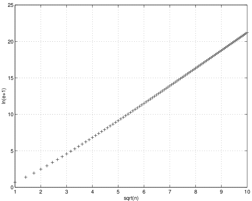
Appendix B Gauß Cubature Rules for
We present computed FS (usually FSMG) Gauß rules for , for (degrees ). For , Mathematica (or a combination of it and some manual substitutions) provides analytic solutions. For higher degrees, only transcendental solutions exist. Instead, we use the matlab program cubature.m to approximate a solution, and we have to trust that an approximation with a small residual corresponds to a transcendental solution. The analytic solutions for low degrees provide good test data for cubature.m. All of the rules presented have been discovered by cubature.m; where possible, analytic solutions have been substituted. Beyond , no solutions at all have been found, but they should be available with sufficient computational effort. For most cases the rules are FSMG from the first structure corresponding to the first minima of the IPP. For , the structure is from the second minima of the first structure. For there is no FSMG rule, but an FSGM rule from the first minima of the second structure is obtained.
- •
, degree . An FSMG rule is :
- •
, degree . An FSMG rule is :
- •
, degree . An FSMG rule is :
- •
, degree . An FSMG rule is :
- •
, degree . An FSMG rule is :
- •
, degree . An FSM rule is :
This rule is not good, as . A (non-unique) FSGM rule is :
- •
, degree . An FSMG rule is :
- •
, degree . An FSMG rule is :
Appendix C C Code
C.1 findec.c
/*
  Find the number of types of equivalence classes e+1, of fully
  symmetric points in n dimensions, by exhaustively enumerating them.
  A UNIX input line "findEC a b" will find e+1 for n = a, ..., b.

  Peter Adams and David  De Wit
  August 1  1993
*/

int string[100], ctr, n;

int checkrep(ind)
int ind;
{
  int repnums[100], rn, i, lv;

  for (i = 0; i < 100; i++)
    repnums[i] = 0;
  repnums[rn = 0] = 1;
  lv = 1;
  for (i = 1; i <= ind; i++) {
    if (string[i] == lv)
      repnums[rn]++;
    else {
      lv = string[i];
      repnums[++rn] = 1;
    }
  }
  for (i = 1; i < rn; i++)
    if (repnums[i] > repnums[i-1])
      return(0);
  return(1);
}

void build(lastv, ind)
int lastv, ind;
{
  int i;

  if (!checkrep(ind)) return;
  ctr++;
  if (ind == n) return;
  string[ind] = lastv;
  build(lastv, ind+1);
  if (lastv < n) {
    string[ind] = lastv + 1;
    build(lastv+1, ind+1);
  }
  string[ind] = 0;
}


main(argc, argv)
char *argv[];
{
  int i;

  printf(" n\t   e+1\n--------------\n", n, ctr);
  for (n = atoi(argv[1]); n <= atoi(argv[2]); n++)
  {
    ctr = 0;
    for (i = 0; i < n; i++)
      string[i] = 0;
    ctr++;
    string[0] = 1;
    build(1, 1);
    printf("%2d\t%6d\n", n, ctr);
  }
}
C.2 ipp.c
/*
    Exhaustively solve the IPP, using the precalculated lower bound for
    $ N $. This is a crude but fast and successful method. The data is
    output, for each m, in terms of increasing structure. Running the
    UNIX "sort" on the output orders it into increasing N, then structure.

    David  De Wit
    August 1 -- August 9  1993
*/

#include <stdio.h>

#define LIMIT   20
#define NUMofM  21

static int NLB[NUMofM] =
{
  0,   6,  14,  26,  38,  50,  74,  86, 110, 138, 162,
     190, 230, 258, 298, 342, 382, 426, 482, 526, 582
};
static int c[4][NUMofM] =
{
  {0, 1, 2, 3, 4, 5, 7, 8, 10, 12, 14, 16, 19, 21, 24, 27, 30, 33, 37, 40, 44},
  {0, 0, 0, 1, 1, 2, 3, 4,  5,  7,  8, 10, 12, 14, 16, 19, 21, 24, 27, 30, 33},
  {0, 0, 0, 0, 0, 0, 1, 1,  2,  3,  4,  5,  7,  8, 10, 12, 14, 16, 19, 21, 24},
  {0, 0, 0, 0, 0, 0, 0, 0,  0,  1,  1,  2,  3,  4,  5,  7,  8, 10, 12, 14, 16}
};
static double alpha[NUMofM] =
{
  0.00, 17.00, 7.00, 4.00, 3.00, 2.30, 1.80, 1.70, 1.45, 1.40, 1.35,
         1.25, 1.20, 1.20, 1.15, 1.13, 1.12, 1.11, 1.09, 1.08, 1.08
};


main()
{
  int     m, K1, K2, K3, K4, K5, K6, N, Nvars, nstruct[NUMofM], NUB[NUMofM];

  for (m = 1; m < NUMofM; m++) {
    nstruct[m] = 0;
    NUB[m] = (int) (alpha[m]*NLB[m]);
    for (K1 = 0; K1 <= 1; K1++)
    for (K2 = 0; K2 <= 1; K2++)
    for (K3 = 0; K3 <= LIMIT; K3++)
    for (K4 = 0; K4 <= 1; K4++)
    for (K5 = 0; K5 <= LIMIT; K5++)
    for (K6 = 0; K6 <= LIMIT; K6++) {
      N = 6*K1 + 12*K2 + 24*K3 + 8*K4 + 24*K5 + 48*K6;
      if (N > NUB[m])
         break;
      if (NLB[m] <= N &
          K1 + K2 + 2*K3 + K4 + 2*K5 + 3*K6 >= c[0][m] &
                           K4 + 2*K5 + 3*K6 >= c[1][m] &
                    2*K3             + 3*K6 >= c[2][m] &
                                       3*K6 >= c[3][m]) {
        Nvars = 2*K1 + 2*K2 + 3*K3 + 2*K4 + 3*K5 + 4*K6;
        printf("$ %2d $ & $ %3d $ & $ %1d $ & $ %1d $ & $ ", m, N, K1, K2);
        printf("%2d $ & $ %1d $ & $ %2d $ & $ ", K3, K4, K5);
        printf("%2d $ & $ %2d $ \\\\\n", K6, Nvars);
        nstruct[m]++;
      }
    }
    printf("\\hline\n %% For m = %d, there are %d structures in the range %d-%d\n\n",
           m, nstruct[m], NLB[m], NUB[m]);
  }
}
C.3 writestar.c
/*
  Write down the system of moment equations as a LaTeX file.  Input is
  m, and a structure K.  Includes the moment data created by the
  Mathematica function U3Moments.M. This code is not watertight!

  David  De Wit
  August 4  --  September 29  1993
*/

#include <stdio.h>
#define    pi    3.141592653589793238462643383280

main(argc, argv)
int  argc;
char *argv[];
{
  int    K[7], m, i, j1, j2, j3, J1, J2, J3, eqno, pflag, nflag;
  double mom[4][6][11];

/* Initialise some variables */
  if (argc == 8) {
    m = atoi(argv[1]);
    for (i = 1; i <= 6; i++)
      K[i] = atoi(argv[i+1]);
  }
  else {
    m = 3;  K[1] = 1;  K[2] = 1;  K[3] = 0;  K[4] = 1;  K[5] = 0;  K[6] = 0;
  }

  mom[0][0][0]  =  4*pi;            mom[0][0][1]  =  4*pi/3;
  mom[0][0][2]  =  4*pi/5;          mom[0][0][3]  =  4*pi/7;
  mom[0][0][4]  =  4*pi/9;          mom[0][0][5]  =  4*pi/11;
  mom[0][0][6]  =  4*pi/13;         mom[0][0][7]  =  4*pi/15;
  mom[0][0][8]  =  4*pi/17;         mom[0][0][9]  =  4*pi/19;
  mom[0][0][10] =  4*pi/21;         mom[0][1][1]  =  4*pi/15;
  mom[0][1][2]  =  4*pi/35;         mom[0][1][3]  =  4*pi/63;
  mom[0][1][4]  =  4*pi/99;         mom[0][1][5]  =  4*pi/143;
  mom[0][1][6]  =  4*pi/195;        mom[0][1][7]  =  4*pi/255;
  mom[0][1][8]  =  4*pi/323;        mom[0][1][9]  =  4*pi/399;
  mom[0][2][2]  =  4*pi/105;        mom[0][2][3]  =  4*pi/231;
  mom[0][2][4]  =  4*pi/429;        mom[0][2][5]  =  4*pi/715;
  mom[0][2][6]  =  4*pi/1105;       mom[0][2][7]  =  4*pi/1615;
  mom[0][2][8]  =  4*pi/2261;       mom[0][3][3]  =  20*pi/3003;
  mom[0][3][4]  =  4*pi/1287;       mom[0][3][5]  =  4*pi/2431;
  mom[0][3][6]  =  4*pi/4199;       mom[0][3][7]  =  4*pi/6783;
  mom[0][4][4]  =  28*pi/21879;     mom[0][4][5]  =  28*pi/46189;
  mom[0][4][6]  =  4*pi/12597;      mom[0][5][5]  =  12*pi/46189;
  mom[1][1][1]  =  4*pi/105;        mom[1][1][2]  =  4*pi/315;
  mom[1][1][3]  =  4*pi/693;        mom[1][1][4]  =  4*pi/1287;
  mom[1][1][5]  =  4*pi/2145;       mom[1][1][6]  =  4*pi/3315;
  mom[1][1][7]  =  4*pi/4845;       mom[1][1][8]  =  4*pi/6783;
  mom[1][2][2]  =  4*pi/1155;       mom[1][2][3]  =  4*pi/3003;
  mom[1][2][4]  =  4*pi/6435;       mom[1][2][5]  =  4*pi/12155;
  mom[1][2][6]  =  4*pi/20995;      mom[1][2][7]  =  4*pi/33915;
  mom[1][3][3]  =  4*pi/9009;       mom[1][3][4]  =  4*pi/21879;
  mom[1][3][5]  =  4*pi/46189;      mom[1][3][6]  =  4*pi/88179;
  mom[1][4][4]  =  28*pi/415701;    mom[1][4][5]  =  4*pi/138567;
  mom[2][2][2]  =  4*pi/5005;       mom[2][2][3]  =  4*pi/15015;
  mom[2][2][4]  =  4*pi/36465;      mom[2][2][5]  =  12*pi/230945;
  mom[2][2][6]  =  4*pi/146965;     mom[2][3][3]  =  4*pi/51051;
  mom[2][3][4]  =  4*pi/138567;     mom[2][3][5]  =  4*pi/323323;
  mom[2][4][4]  =  4*pi/415701;     mom[3][3][3]  =  20*pi/969969;
  mom[3][3][4]  =  20*pi/2909907;

/* Introduce the output */
  printf("Output from running ‘writestar’: m = %d, ", m);
  printf("K = %d %d %d %d %d %d:\n\n", K[1], K[2], K[3], K[4], K[5], K[6]);

/* Deal with Subsystem I */
  printf("\\be\n\%% Subsystem I/1:\n");
  pflag = 0;  eqno++;
  printf("  I \\[ 1 \\]\n  \\eq\n  ");
  if (K[1]) {
    pflag = 1;  printf("6 a_1");
  }
  if (K[2]) {
    if (pflag) printf(" +\n  ");  pflag = 1;
    printf("12 b_1");
  }
  if (K[3]) {
    if (pflag) printf(" +\n  ");  pflag = 1;
    if (K[3] > 1)
      printf("24 \\sum_{i=1}^{%d} c_i", K[3]);
    else
      printf("24 c_1");
  }
  if (K[4]) {
    if (pflag) printf(" +\n  ");  pflag = 1;
    printf("8 d_1");
  }
  if (K[5]) {
    if (pflag) printf(" +\n  ");  pflag = 1;
    if (K[5] > 1)
      printf("24 \\sum_{i=1}^{%d} e_i", K[5]);
    else
      printf("24 e_1");
  }
  if (K[6]) {
    if (pflag) printf(" +\n  ");  pflag = 1;
    if (K[6] > 1)
      printf("48 \\sum_{i=1}^{%d} f_i", K[6]);
    else
      printf("48 f_1");
  }
  printf("\n  \\\\\n");

  printf("\%% Subsystem I/2:\n");
  for (j1 = 1; j1 <= m; j1++)
  {
    J1 = 2*j1;  eqno++;
    printf("  I \\[ x^{%d} \\]\n  \\eq\n  ", J1);
    if (K[1]) {
      pflag = 1;  printf("2 a_1 \\alpha_1^{%d}", J1);
    }
    if (K[2]) {
      if (pflag) printf(" +\n  ");  pflag = 1;
      printf("8 b_1 \\beta_1^{%d}", J1);
    }
    if (K[3]) {
      if (pflag) printf(" +\n  ");  pflag = 1;
      if (K[3] > 1)
        printf("8 \\sum_{i=1}^{%d} c_i \\( \\gamma_i^{%d} + \\delta_i^{%d} \\)", K[3], J1, J1);
      else
        printf("8 c_1 \\( \\gamma_1^{%d} + \\delta_1^{%d} \\)", J1, J1);
    }
    if (K[4]) {
      if (pflag) printf(" +\n  ");  pflag = 1;
      printf("8 d_1 \\epsilon_1^{%d}", J1);
    }
    if (K[5]) {
      if (pflag) printf(" +\n  ");  pflag = 1;
      if (K[5] > 1)
        printf("8 \\sum_{i=1}^{%d} e_i \\( 2 \\zeta_i^{%d} + \\eta_i^{%d} \\)", K[5], J1, J1);
      else
        printf("8 e_1 \\( 2 \\zeta_1^{%d} + \\eta_1^{%d} \\)", J1, J1);
    }
    if (K[6]) {
      if (pflag) printf(" +\n  ");  pflag = 1;
      if (K[6] > 1) {
        printf("16 \\sum_{i=1}^{%d} f_i ", K[6]);
        printf("\\( \\theta_i^{%d} + \\mu_i^{%d} + \\lambda_i^{%d} \\)", J1, J1, J1);
      }
      else
        printf("16 f_1 \\( \\theta_1^{%d} + \\mu_1^{%d} + \\lambda_1^{%d} \\)", J1, J1, J1);
    }
    printf("\n  \\\\\n");
  }

/* Deal with Subsystem II */
  if (m >= 2) {
  printf("\%% Subsystem II:\n");
  for (j1 = 1; j1 <= m; j1++)
  for (j2 = j1; j2 <= m-j1; j2++) {
    pflag = 0;  J1 = 2*j1;  J2 = 2*j2;
    eqno++;
    printf("  I \\[ x^{%d} y^{%d} \\]\n  \\eq\n  ", J1, J2);
    if (K[2]) {
      pflag = 1;  printf("4 b_1 \\beta_1^{%d}", J1+J2);
    }
    if (K[3]) {
      if (pflag) printf(" +\n  ");  pflag = 1;
      if (K[3] > 1) {
        printf("4 \\sum_{i=1}^{%d} c_i \\( \\gamma_i^{%d} \\delta_i^{%d} ", K[3], J1, J2);
        printf("+ \\gamma_i^{%d} \\delta_i^{%d} \\)", J2, J1);
      }
      else {
        printf("4 c_1 \\( \\gamma_1^{%d} \\delta_1^{%d} ", J1, J2);
        printf("+ \\gamma_1^{%d} \\delta_1^{%d} \\)", J2, J1);
      }
    }
    if (K[4]) {
      if (pflag) printf(" +\n  ");  pflag = 1;
      printf("8 d_1 \\epsilon_1^{%d}", J1+J2);
    }
    if (K[5]) {
      if (pflag) printf(" +\n  ");  pflag = 1;
      if (K[5] > 1) {
        printf("8 \\sum_{i=1}^{%d} e_i \\( \\zeta_i^{%d} + ", K[5], J1+J2);
        printf("\\zeta_i^{%d} \\eta_i^{%d} + \\zeta_i^{%d} \\eta_i^{%d} \\)", J1, J2, J2, J1);
      }
      else {
        printf("8 e_1 \\( \\zeta_1^{%d} + ", J1+J2);
        printf("\\zeta_1^{%d} \\eta_1^{%d} + \\zeta_1^{%d} \\eta_1^{%d} \\)", J1, J2, J2, J1);
      }
    }
    if (K[6]) {
      if (pflag) printf(" +\n  ");  pflag = 1;
      if (K[6] > 1) {
        printf("  \\\\\n  & & \\qquad8 \\sum_{i=1}^{%d} f_i \\( ", K[6]);
        printf("\\theta_i^{%d} \\mu_i^{%d} + ", J1, J2);
        printf("\\theta_i^{%d} \\mu_i^{%d} + ", J2, J1);
        printf("\\theta_i^{%d} \\lambda_i^{%d} + ", J1, J2);
        printf("\\theta_i^{%d} \\lambda_i^{%d} +", J2, J1);
        printf("\\mu_i^{%d} \\lambda_i^{%d} + ", J1, J2);
        printf("\\mu_i^{%d} \\lambda_i^{%d} \\)", J2, J1);
      }
      else {
        printf("  \\\\\n  & & \\qquad8 f_1 \\( ");
        printf("\\theta_1^{%d} \\mu_1^{%d} + ", J1, J2);
        printf("\\theta_1^{%d} \\mu_1^{%d} + ", J2, J1);
        printf("\\theta_1^{%d} \\lambda_1^{%d} + ", J1, J2);
        printf("\\theta_1^{%d} \\lambda_1^{%d} + ", J2, J1);
        printf("\\mu_1^{%d} \\lambda_1^{%d} + ", J1, J2);
        printf("\\mu_1^{%d} \\lambda_1^{%d} \\)", J2, J1);
      }
    }
    printf("\n  \\\\\n");
  } }

/* Deal with Subsystem III */
  if (m >= 3) {
  printf("\%% Subsystem III:\n");
  for (j1 = 1; j1 <= m; j1++)
  for (j2 = j1; j2 <= m-j1; j2++)
  for (j3 = j2; j3 <= m-j1-j2; j3++) {
    pflag = 0;  J1 = 2*j1;  J2 = 2*j2;  J3 = 2*j3;  eqno++;
    printf("  I \\[ x^{%d} y^{%d} z^{%d} \\]\n  \\eq\n  ", J1, J2, J3);
    if (K[4]) {
      pflag = 1;  printf("8 d_1 \\epsilon_1^{%d}", J1+J2+J3);
    }
    if (K[5]) {
      if (pflag) printf(" +\n  ");  pflag = 1;
      if (K[5] > 1) {
        printf("8 \\sum_{i=1}^{%d} e_i \\( \\zeta_i^{%d} \\eta_i^{%d} + ", K[5], J1+J2, J3);
        printf("\\zeta_i^{%d} \\eta_i^{%d} + ", J1+J3, J2);
        printf("\\zeta_i^{%d} \\eta_i^{%d} \\)", J2+J3, J1);
      }
      else {
        printf("8 e_1 \\( \\zeta_1^{%d} \\eta_1^{%d} + ", J1+J2, J3);
        printf("\\zeta_1^{%d} \\eta_1^{%d} + ", J1+J3, J2);
        printf("\\zeta_1^{%d} \\eta_1^{%d} \\)", J2+J3, J1);
      }
    }
    if (K[6]) {
      if (pflag) printf(" +\n  ");  pflag = 1;
      if (K[6] > 1) {
        printf("  \\\\\n  & & \\qquad8 \\sum_{i=1}^{%d} f_i \\( ", K[6]);
        printf("\\theta_i^{%d} \\mu_i^{%d} \\lambda_i^{%d} + ", J1, J2, J3);
        printf("\\theta_i^{%d} \\mu_i^{%d} \\lambda_i^{%d} + ", J1, J3, J2);
        printf("\\theta_i^{%d} \\mu_i^{%d} \\lambda_i^{%d} + ", J2, J1, J3);
        printf("\\theta_i^{%d} \\mu_i^{%d} \\lambda_i^{%d} + ", J2, J3, J1);
        printf("\\theta_i^{%d} \\mu_i^{%d} \\lambda_i^{%d} + ", J3, J1, J2);
        printf("\\theta_i^{%d} \\mu_i^{%d} \\lambda_i^{%d} \\)", J3, J2, J1);
      }
      else {
        printf("  \\\\\n  & & \\qquad8 f_1 \\( ");
        printf("\\theta_1^{%d} \\mu_1^{%d} \\lambda_1^{%d} + ", J1, J2, J3);
        printf("\\theta_1^{%d} \\mu_1^{%d} \\lambda_1^{%d} + ", J1, J3, J2);
        printf("\\theta_1^{%d} \\mu_1^{%d} \\lambda_1^{%d} + ", J2, J1, J3);
        printf("\\theta_1^{%d} \\mu_1^{%d} \\lambda_1^{%d} + ", J2, J3, J1);
        printf("\\theta_1^{%d} \\mu_1^{%d} \\lambda_1^{%d} + ", J3, J1, J2);
        printf("\\theta_1^{%d} \\mu_1^{%d} \\lambda_1^{%d} \\)", J3, J2, J1);
      }
    }
    printf("\n  \\\\\n");
  } }

  nflag = 0;
  printf("\%% Also Sprach:\n");
  if (K[1]) {
    printf("  1\n  \\eq\n  \\alpha_1\n");  nflag = 1;  eqno++;
  }
  if (K[2]) {
    if (nflag) printf("  \\\\\n");  nflag = 1;
    printf("  1/\\sqrt{2}\n  \\eq\n  \\beta_1\n");  eqno++;
  }
  if (K[3]) {
    if (nflag) printf("  \\\\\n");  nflag = 1;
    if (K[3] > 1)
      printf("  1\n  \\eq\n  \\gamma_i^2 + \\delta_i^2 \\qquad i = 1, \\dots, %d\n", K[3]);
    else
      printf("  1\n  \\eq\n  \\gamma_1^2 + \\delta_1^2\n");
    eqno += K[3];
  }
  if (K[4]) {
    if (nflag) printf("  \\\\\n");  nflag = 1;
    printf("  1/\\sqrt{3}\n  \\eq\n  \\epsilon_1\n");  eqno++;
  }
  if (K[5]) {
    if (nflag) printf("  \\\\\n");  nflag = 1;
    if (K[5] > 1)
      printf("  1\n  \\eq\n  2 \\zeta_i^2 + \\eta_i^2 \\qquad i = 1, \\dots, %d\n", K[5]);
    else
      printf("  1\n  \\eq\n  2 \\zeta_1^2 + \\eta_1^2\n");
    eqno += K[5];
  }
  if (K[6]) {
    if (nflag) printf("  \\\\\n");  nflag = 1;
    if (K[6] > 1) {
      printf("  1\n  \\eq\n  \\theta_i^2 + \\mu_i^2 + \\lambda_i^2 ");
      printf("\\qquad i = 1, \\dots, %d\n", K[6]);
    }
    else
      printf("  1\n  \\eq\n  \\theta_1^2 + \\mu_1^2 + \\lambda_1^2\n");
    eqno += K[6];
  }
  printf("\\ee\n\nThere are a total of %d equations.\n\n", eqno);
}
Output from running ‘writestar’: m = 4, K = 1 0 1 1 0 0:
There are a total of 14 equations.
Appendix D MATLAB Code
D.1 Gauß Rules
D.1.1 cubature.m
% Solve the system (*) of moment equations, for input parameters
% m and K, to obtain a cubature rule of degree 2m+1.
%
%  David  De Wit
%  September 20  --  October 27  1993


function x = cubature(m, j, t)

format compact;      format long

if (m == 1)
  K = [1 0 0 0 0 0];
elseif (m == 2)
  K = [1 0 0 1 0 0];
elseif (m == 3)
  K = [1 1 0 1 0 0];
elseif (m == 4)
% K = [1 0 0 1 1 0];
  K = [1 0 1 1 0 0];
elseif (m == 5)
  K = [1 1 0 1 1 0];
elseif (m == 6)
  K = [1 1 1 1 1 0];
% K = [1 0 1 0 2 0];
elseif (m == 7)
  K = [1 0 1 1 2 0];
elseif (m == 8)
  K = [1 0 1 1 3 0];
elseif (m == 9)
  K = [1 1 0 1 3 1];
% K = [1 1 1 1 2 1];
elseif (m == 10)
  K = [1 1 1 1 3 1];
% K = [1 1 2 1 2 1];
end

M = [2 2 3 2 3 4]’;
L(1) = 0;
for i = 2:6
  L(i) = L(i-1) + M(i-1)*K(i-1);
end

x0 = rand(K*M,1);
if (K(1)), x0(L(1)+2) = 1; end
if (K(2)), x0(L(2)+2) = 1/sqrt(2); end
if (K(4)), x0(L(4)+2) = 1/sqrt(3); end

options = [1 eps eps 0 1];  options(14) = 10000;

%  Pass the values to the solution routine.
x = fsolve(’momenteq’, x0, options, [], m, K, L);

disp(’m, j, t, K are:’); disp([m j t K]);

%  Decode the resulting x into known variables:
if (K(1))
  a = x(1), alpha = x(2)
end
if (K(2))
 b = x(L(2)+1), beta = x(L(2)+2)
end
if (K(3))
  c       = x(L(3)+1:L(3)+K(3))
  gamma   = x(L(3)+K(3)+1:L(3)+2*K(3));    delta = x(L(3)+2*K(3)+1:L(3)+3*K(3))
end
if (K(4))
  d = x(L(4)+1), epsilon = x(L(4)+2)
end
if (K(5))
  e       = x(L(5)+1:L(5)+K(5))
  zeta    = x(L(5)+K(5)+1:L(5)+2*K(5));      eta = x(L(5)+2*K(5)+1:L(5)+3*K(5))
end
if (K(6))
  f       = x(L(6)+1:L(6)+K(6));           theta = x(L(6)+K(6)+1:L(6)+2*K(6))
  mu      = x(L(6)+2*K(6)+1:L(6)+3*K(6)); lambda = x(L(6)+3*K(6)+1:L(6)+4*K(6))
end
D.1.2 momenteq.c
/*
  C code that compiles into a MATLAB .mex file that ‘evaluates’
  the moment equations (*).

  David  De Wit and Martin Sharry and Peter Adams
  September 24  --  September 29  1993
*/


#include <math.h>
#include "mex.h"

/* Input and Output Arguments */

#define  x_IN  prhs[0]
#define  m_IN  prhs[1]
#define  K_IN  prhs[2]
#define  L_IN  prhs[3]
#define  F_OUT  plhs[0]

static int Neq[10] = {2, 4, 7, 11, 16, 23, 31, 41, 53, 67};
static int M[6] = {2, 2, 3, 2, 3, 4};

mexFunction(nlhs, plhs, nrhs, prhs)
int    nlhs, nrhs;
Matrix *plhs[], *prhs[];
{
  double *F, *x, m, *K, *L;
  int    i, mm;

  /* Check for proper number of arguments */
  if (nrhs != 4) {
    mexErrMsgTxt("momenteq requires four input arguments.");
  } else if (nlhs > 1) {
    mexErrMsgTxt("momenteq requires one output argument.");
  }

  /* Assign pointers to the various parameters */

  x = mxGetPr(x_IN);  m = mxGetScalar(m_IN);
  K = mxGetPr(K_IN);  L = mxGetPr(L_IN);

  mm = Neq[(int) m - 1];
  for (i = 0; i < 6; i++)
    mm += K[i]*(M[i] - 1);
  F_OUT = mxCreateFull(mm, 1, REAL);
  F = mxGetPr(F_OUT);

  momenteq(F, x, m, K, L);
}


#define  pi  3.141592653589793238462643383280
double   mom[4][6][11];

void setmom()
{
  mom[0][0][0]  =  4*pi;            mom[0][0][1]  =  4*pi/3;
  mom[0][0][2]  =  4*pi/5;          mom[0][0][3]  =  4*pi/7;
  mom[0][0][4]  =  4*pi/9;          mom[0][0][5]  =  4*pi/11;
  mom[0][0][6]  =  4*pi/13;         mom[0][0][7]  =  4*pi/15;
  mom[0][0][8]  =  4*pi/17;         mom[0][0][9]  =  4*pi/19;
  mom[0][0][10] =  4*pi/21;         mom[0][1][1]  =  4*pi/15;
  mom[0][1][2]  =  4*pi/35;         mom[0][1][3]  =  4*pi/63;
  mom[0][1][4]  =  4*pi/99;         mom[0][1][5]  =  4*pi/143;
  mom[0][1][6]  =  4*pi/195;        mom[0][1][7]  =  4*pi/255;
  mom[0][1][8]  =  4*pi/323;        mom[0][1][9]  =  4*pi/399;
  mom[0][2][2]  =  4*pi/105;        mom[0][2][3]  =  4*pi/231;
  mom[0][2][4]  =  4*pi/429;        mom[0][2][5]  =  4*pi/715;
  mom[0][2][6]  =  4*pi/1105;       mom[0][2][7]  =  4*pi/1615;
  mom[0][2][8]  =  4*pi/2261;       mom[0][3][3]  =  20*pi/3003;
  mom[0][3][4]  =  4*pi/1287;       mom[0][3][5]  =  4*pi/2431;
  mom[0][3][6]  =  4*pi/4199;       mom[0][3][7]  =  4*pi/6783;
  mom[0][4][4]  =  28*pi/21879;     mom[0][4][5]  =  28*pi/46189;
  mom[0][4][6]  =  4*pi/12597;      mom[0][5][5]  =  12*pi/46189;
  mom[1][1][1]  =  4*pi/105;        mom[1][1][2]  =  4*pi/315;
  mom[1][1][3]  =  4*pi/693;        mom[1][1][4]  =  4*pi/1287;
  mom[1][1][5]  =  4*pi/2145;       mom[1][1][6]  =  4*pi/3315;
  mom[1][1][7]  =  4*pi/4845;       mom[1][1][8]  =  4*pi/6783;
  mom[1][2][2]  =  4*pi/1155;       mom[1][2][3]  =  4*pi/3003;
  mom[1][2][4]  =  4*pi/6435;       mom[1][2][5]  =  4*pi/12155;
  mom[1][2][6]  =  4*pi/20995;      mom[1][2][7]  =  4*pi/33915;
  mom[1][3][3]  =  4*pi/9009;       mom[1][3][4]  =  4*pi/21879;
  mom[1][3][5]  =  4*pi/46189;      mom[1][3][6]  =  4*pi/88179;
  mom[1][4][4]  =  28*pi/415701;    mom[1][4][5]  =  4*pi/138567;
  mom[2][2][2]  =  4*pi/5005;       mom[2][2][3]  =  4*pi/15015;
  mom[2][2][4]  =  4*pi/36465;      mom[2][2][5]  =  12*pi/230945;
  mom[2][2][6]  =  4*pi/146965;     mom[2][3][3]  =  4*pi/51051;
  mom[2][3][4]  =  4*pi/138567;     mom[2][3][5]  =  4*pi/323323;
  mom[2][4][4]  =  4*pi/415701;     mom[3][3][3]  =  20*pi/969969;
  mom[3][3][4]  =  20*pi/2909907;
}

momenteq(F, x, m, K, L)
double  F[], x[], m, K[], L[];
{
  int        iK[6], iL[6], i, im, j1, j2, j3, p;
  double     *a, *alpha, *b, *beta, *c,  *gammah, *delta, *d, *epsilon,
             *e, *zeta, *eta, *f, *theta, *mu, *lambda, J1, J2, J3;
  static int havesetmom = 0;

  if(!havesetmom) {
    setmom();  havesetmom = 1;
  }
  im = (int) m;
  for (i = 0; i < 6; i++) {
    iK[i] = (int) K[i];  iL[i] = (int) L[i];
  }

  a       = (double *) malloc ( iK[0] * sizeof(double) );
  alpha   = (double *) malloc ( iK[0] * sizeof(double) );
  b       = (double *) malloc ( iK[1] * sizeof(double) );
  beta    = (double *) malloc ( iK[1] * sizeof(double) );
  c       = (double *) malloc ( iK[2] * sizeof(double) );
  gammah  = (double *) malloc ( iK[2] * sizeof(double) );
  delta   = (double *) malloc ( iK[2] * sizeof(double) );
  d       = (double *) malloc ( iK[3] * sizeof(double) );
  epsilon = (double *) malloc ( iK[3] * sizeof(double) );
  e       = (double *) malloc ( iK[4] * sizeof(double) );
  zeta    = (double *) malloc ( iK[4] * sizeof(double) );
  eta     = (double *) malloc ( iK[4] * sizeof(double) );
  f       = (double *) malloc ( iK[5] * sizeof(double) );
  theta   = (double *) malloc ( iK[5] * sizeof(double) );
  mu      = (double *) malloc ( iK[5] * sizeof(double) );
  lambda  = (double *) malloc ( iK[5] * sizeof(double) );

  for (i = 0; i < iK[0]; i++) {
    a[i] = x[iL[0]+i];   alpha[i] = x[iL[0]+1*iK[0]+i];
  }
  for (i = 0; i < iK[1]; i++) {
   b[i] = x[iL[1]+i];     beta[i] = x[iL[1]+1*iK[1]+i];
  }
  for (i = 0; i < iK[2]; i++) {
    c[i] = x[iL[2]+i];  gammah[i] = x[iL[2]+1*iK[2]+i]; delta[i] = x[iL[2]+2*iK[2]+i];
  }
  for (i = 0; i < iK[3]; i++) {
    d[i] = x[iL[3]+i]; epsilon[i] = x[iL[3]+1*iK[3]+i];
  }
  for (i = 0; i < iK[4]; i++) {
    e[i] = x[iL[4]+i];    zeta[i] = x[iL[4]+1*iK[4]+i]; eta[i] = x[iL[4]+2*iK[4]+i];
  }
  for (i = 0; i < iK[5]; i++) {
    f[i] = x[iL[5]+i];   theta[i] = x[iL[5]+1*iK[5]+i]; mu[i] = x[iL[5]+2*iK[5]+i];
                        lambda[i] = x[iL[5]+3*iK[5]+i];
  }

/* Subsystem I */
  F[p = 0] = - mom[0][0][0];
  for (i = 0; i < iK[0]; i++) F[p] +=  6*a[i];
  for (i = 0; i < iK[1]; i++) F[p] += 12*b[i];
  for (i = 0; i < iK[2]; i++) F[p] += 24*c[i];
  for (i = 0; i < iK[3]; i++) F[p] +=  8*d[i];
  for (i = 0; i < iK[4]; i++) F[p] += 24*e[i];
  for (i = 0; i < iK[5]; i++) F[p] += 48*f[i];

  for (j1 = 1; j1 <= im; j1++) {
    J1 = 2.0*j1;
    F[++p] = - mom[0][0][j1];
    for (i = 0; i < iK[0]; i++)
      F[p] +=  2*a[i]*pow(alpha[i],J1);
    for (i = 0; i < iK[1]; i++)
      F[p] +=  8*b[i]*pow(beta[i],J1);
    for (i = 0; i < iK[2]; i++)
      F[p] +=  8*c[i]*(pow(gammah[i],J1) + pow(delta[i],J1));
    for (i = 0; i < iK[3]; i++)
      F[p] +=  8*d[i]*pow(epsilon[i],J1);
    for (i = 0; i < iK[4]; i++)
      F[p] +=  8*e[i]*(2*pow(zeta[i],J1) + pow(eta[i],J1));
    for (i = 0; i < iK[5]; i++)
      F[p] += 16*f[i]*(pow(theta[i],J1) + pow(mu[i],J1) + pow(lambda[i],J1));
  }

/* Subsystem II  */
  if (im >= 2)
    for (j1 = 1; j1 <= im; j1++) {
      J1 = 2.0*j1;
      for (j2 = j1; j2 <= im-j1; j2++) {
        J2 = 2.0*j2;
        F[++p] = - mom[0][j1][j2];
        for (i = 0; i < iK[1]; i++)
          F[p] +=  4*b[i]*pow(beta[i],J1+J2);
        for (i = 0; i < iK[2]; i++)
          F[p] +=  4*c[i]*(
                   pow(gammah[i],J1)*pow(delta[i],J2) + pow(gammah[i],J2)*pow(delta[i],J1));
        for (i = 0; i < iK[3]; i++)
          F[p] +=  8*d[i]*pow(epsilon[i],J1+J2);
        for (i = 0; i < iK[4]; i++)
          F[p] +=  8*e[i]*(
                   pow(zeta[i],J1+J2) +
                   pow(zeta[i],J1)*pow(eta[i],J2) +
                   pow(zeta[i],J2)*pow(eta[i],J1));
        for (i = 0; i < iK[5]; i++)
          F[p] += 8*f[i]*(
                  pow(theta[i],J1)*pow(mu[i],J2) + pow(theta[i],J2)*pow(mu[i],J1) +
                  pow(theta[i],J1)*pow(lambda[i],J2) + pow(theta[i],J2)*pow(lambda[i],J1) +
                  pow(mu[i],J1)*pow(lambda[i],J2) + pow(mu[i],J2)*pow(lambda[i],J1));
    } }

/* Subsystem III  */
  if (im >= 3)
    for (j1 = 1; j1 <= im; j1++) {
      J1 = 2.0*j1;
      for (j2 = j1; j2 <= im-j1; j2++) {
        J2 = 2.0*j2;
        for (j3 = j2; j3 <= im-j1-j2; j3++) {
          J3 = 2.0*j3;
          p++;
          F[p] = - mom[j1][j2][j3];
          for (i = 0; i < iK[3]; i++)
            F[p] +=  8*d[i]*pow(epsilon[i],J1+J2+J3);
          for (i = 0; i < iK[4]; i++)
            F[p] +=  8*e[i]*(
                     pow(zeta[i],J1+J2)*pow(eta[i],J3) +
                     pow(zeta[i],J1+J3)*pow(eta[i],J2) +
                     pow(zeta[i],J2+J3)*pow(eta[i],J1));
          for (i = 0; i < iK[5]; i++)
            F[p] += 8*f[i]*(
                    pow(theta[i],J1)*pow(mu[i],J2)*pow(lambda[i],J3) +
                    pow(theta[i],J1)*pow(mu[i],J3)*pow(lambda[i],J2) +
                    pow(theta[i],J2)*pow(mu[i],J1)*pow(lambda[i],J3) +
                    pow(theta[i],J2)*pow(mu[i],J3)*pow(lambda[i],J1) +
                    pow(theta[i],J3)*pow(mu[i],J1)*pow(lambda[i],J2) +
                    pow(theta[i],J3)*pow(mu[i],J2)*pow(lambda[i],J1));
    } } };

/* Also Sprach  */
  for (i = 0; i < iK[0]; i++)
    F[++p] = alpha[i] - 1;
  for (i = 0; i < iK[1]; i++)
    F[++p] = beta[i] - 1/sqrt(2.0);
  for (i = 0; i < iK[2]; i++)
    F[++p] = pow(gammah[i],2.0) + pow(delta[i],2.0) - 1;
  for (i = 0; i < iK[3]; i++)
    F[++p] = epsilon[i] - 1/sqrt(3.0);
  for (i = 0; i < iK[4]; i++)
    F[++p] = 2*pow(zeta[i],2.0) + pow(eta[i],2.0) - 1;
  for (i = 0; i < iK[5]; i++)
    F[++p] = pow(theta[i],2.0) + pow(mu[i],2.0) + pow(lambda[i],2.0) - 1;

  free(a); free(alpha); free(b); free(beta); free(c); free(gammah); free(delta);
  free(d); free(epsilon); free(e); free(zeta); free(eta);
  free(f); free(theta); free(mu); free(lambda);
}
D.2 Product Rules
D.2.1 u3prod.m
function [y, A] = u3prod(M)

% function [y, A] = u3prod(M)
%
% Product rule cubature for U_3. On input, M is the number of points in
% the basic rules. Gives a Gauss product rule of degree 2M - 1 on 2 M^2
% Cartesian points -+ y, with weights A. y is an M^2 x 3 matrix, A an
% M^2 column vector.  To obtain a rule of degree p, a rule on
% (p + 1)^2 / 2 points is required.  Requires gauss.m, which returns
% the points and weights of the $ M $-point 1D Gauss-Legendre rule.
% See Stroud (1971), p 41.
%
% David  De Wit
% February 11  -  February 12  1993

if ~exist(’M’), M = 5; end

[yG, AG] = gauss(M,-1,1);
j = [1:M]’;

yCI = cos((2*j - 1)*pi/(2*M));    ACI = ones(size(j))*pi/M;

y1 = sqrt(1 - yCI.^2) * sqrt(1 - yG.^2)’;
y2 = yCI * sqrt(1 - yG.^2)’;
y3 = ones(M,1) * yG’;
A = ACI * AG’;

y = [y1(:) y2(:) y3(:)];          A = A(:);

plot3(y(:,1),y(:,2),y(:,3),’+r’);

% Test by integrating all functions of x, y and z of degree < M.
% Works beautifully!

% t = M-1;        m = 1;
% for j = 0:t, for k = j:t, for l = k:t
%   if (j+k+l <= t)
%     i = [j k l];
%     tabi(m,:) = i;
%     table(m) = 2*(y(:,1).^(2*i(1)).*y(:,2).^(2*i(2)) ...
%                .*y(:,3).^(2*i(3)))’*A - ...
%                2*prod(gamma(i+1/2))/gamma(3/2+sum(i));
%     m = m + 1;
%   end
% end, end, end
% tabi
% table’
% m
D.2.2 gauss.m
function [x, w] = gauss(n, a, b)

% function [x, w] = gauss(n, a, b)
% Returns {x, w}, the weights and of the n-point Gauss- Legendre
% quadrature rule on the interval  [a, b]
%
% Graeme Chandler 1992

if (n==1)
    x = (a+b)/2 ; w = b-a ; return
end

m = 1:2:2*n-1 ;
m = (1:n-1) ./ sqrt(m(1:n-1).*m(2:n));   %  m is off-diagonal of matrix
[w, x] = eig(diag(m,-1)+diag(m,1));      %  Find spectrum of matrix
x = (a+b)/2 + ((b-a)/2)*diag(x);         %  x are the eigenvalues
w = (b-a)*(w(1,:).^2)’;                  %  w from first components
[x, m] = sort(x);        w = w(m);       %  ascending order
Appendix E Mathematica Code
E.1 IPPBasicSolution.M
(*
  Find basic solutions to the IPP, ignoring the integer requirement,
  for m = 1, ..., 20.

  David  De Wit
  August 4  1993
*)

mmax = 20
A = {
  { 1,  1,  2,  1,  2,  3},
  { 0,  0,  0,  1,  2,  3},
  { 0,  0,  2,  0,  0,  3},
  { 0,  0,  0,  0,  0,  3},
  {-1,  0,  0,  0,  0,  0},
  { 0, -1,  0,  0,  0,  0},
  { 0,  0,  0, -1,  0,  0}
}
c = {6, 12, 24, 8, 24, 48}
b = Transpose[ {
  { 0,  1,  2,  3,  4,  5,  7,  8, 10, 12, 14, 16, 19, 21, 24, 27, 30, 33, 37, 40, 44},
  { 0,  0,  0,  1,  1,  2,  3,  4,  5,  7,  8, 10, 12, 14, 16, 19, 21, 24, 27, 30, 33},
  { 0,  0,  0,  0,  0,  0,  1,  1,  2,  3,  4,  5,  7,  8, 10, 12, 14, 16, 19, 21, 24},
  { 0,  0,  0,  0,  0,  0,  0,  0,  0,  1,  1,  2,  3,  4,  5,  7,  8, 10, 12, 14, 16},
  {-1, -1, -1, -1, -1, -1, -1, -1, -1, -1, -1, -1, -1, -1, -1, -1, -1, -1, -1, -1, -1},
  {-1, -1, -1, -1, -1, -1, -1, -1, -1, -1, -1, -1, -1, -1, -1, -1, -1, -1, -1, -1, -1},
  {-1, -1, -1, -1, -1, -1, -1, -1, -1, -1, -1, -1, -1, -1, -1, -1, -1, -1, -1, -1, -1}
}]
sol = Table[0, {i, mmax+1}, {j, 6}]
nmin = Table[0, {i, mmax+1}]
For [m = 1, m <= mmax+1, m++,
  sol[[m]] = LinearProgramming[c, A, b[[m]]]
]
nmin = c . Transpose[sol]

stmp = OpenWrite["IPPBasicSolnData.tex.bak"]
For [m = 1, m <= mmax+1, m++,
  WriteString[{"stdout", stmp}, "$ ", m-1, " $ & $ ", nmin[[m]]
  ];
  For [n = 1, n <=6, n++,
    WriteString [{"stdout", stmp}, " $ & $ ", InputForm[sol[[m,n]]]
    ];
  ];
  WriteString[ {"stdout", stmp}, " $ \\\\\n" ];
];
Close[stmp]
E.2 U3Moments.M
(*
  Find the moments for integrals of polynomials over U_3, and output
  into a file suitable for inclusion as a LaTeX table. The output is
  also included in the programs momenteq.c and writestar.c. The method
  is extremely crude, but operational!

  David  De Wit
  August 4  -- August 12  1993
*)

stmp = OpenWrite["U3MomentData.tex"]
For [j1 = 0, j1 <= 10, j1++,
For [j2 = j1, j2 <= 10-j1, j2++,
For [j3 = j2, j3 <= 10-j2-j1, j3++,
  f[t_] = (Cos[t])^(2 j1) (Sin[t])^(2 j2);
  g[t_] = (Cos[t])^(2 j1 + 2 j2 + 1) (Sin[t])^(2 j3);
  Int = Integrate[g[t], {t,-Pi/2,Pi/2}] Integrate[f[t], {t,-Pi,Pi}];
  WriteString[
    {"stdout", stmp},
    "$ ", j1, " $ & $ ", j2, " $ & $ ", j3, " $ & $ ", InputForm[Int], " $ \\\\", "\n"]
] ] ]
Close[stmp]
References
- [1] Kendall E. Atkinson. Numerical integration on the sphere. Journal of the Australian Mathematical Society (Series B), 23:332–347, 1982.
- [2] Kendall E. Atkinson. The numerical solution of Laplace’s equation in three dimensions. SIAM Journal on Numerical Analysis, 19(2):263–274, April 1982.
- [3] B. W. Clare and D. L. Keppert. The closest packing of equal circles on a sphere. Proceedings of the Royal Society of London, A 405:329–344, 1986.
- [4] B. W. Clare and D. L. Keppert. The optimal packing of circles on a sphere. Journal of Mathematical Chemistry, 6:325–349, 1991.
- [5] David Cox, John Little, and Donal O’Shea. Ideals, Varieties, and Algorithms. Undergraduate Texts in Mathematics. Springer-Verlag, New York, Berlin, etc., 1992.
- [6] Philip J. Davis and Philip Rabinowitz. Methods of Numerical Integration. Academic Press, Orlando, 2nd edition, 1984.
- [7] Ernest William Hobson. The Theory of Spherical and Ellipsoidal Harmonics. Cambridge University Press, Cambridge, 1931.
- [8] Patrick Keast. Some fully symmetric quadrature formulae for product spaces. Journal of the Institute of Mathematics and its Applications, 23:251–264, 1979.
- [9] Patrick Keast. Cubature formulas for the surface of the sphere. Journal of Computational and Applied Mathematics, 17(1–2):151–172, 1987.
- [10] Patrick Keast and Julio C. Diaz. Fully symmetric integration formulas for the surface of the sphere in dimensions. SIAM Journal on Numerical Analysis, 20(2):406–419, April 1983.
- [11] Patrick Keast and James N. Lyness. On the structure of fully symmetric multidimensional quadrature rules. SIAM Journal on Numerical Analysis, 16(1):11–29, February 1979.
- [12] Rainer Kress. Linear Integral Equations, volume 82 of Applied Mathematical Sciences. Springer-Verlag, Berlin, Heidelberg, 1989.
- [13] Vladimir Ivanovich Krylov. Approximate Calculation of Integrals. Macmillan, New York, 1962. Translated from the first Russian edition (1959) by A. H. Stroud.
- [14] V. I. Lebedev. Quadratures on a sphere. USSR Computational Mathematics and Mathematical Physics, 16(2):10–24, 1976. Translated from the Russian original, Zhurnal Vychistlitel’noi Matematiki i Matematicheskoi Fiziki, 16(2):293–306, 1976.
- [15] James N. Lyness. Symmetric integration rules for hypercubes. I. Error coefficients. Mathematics of Computation, 19:260–276, 1965.
- [16] James N. Lyness and Ian H. Sloan. Some properties of rank-2 lattice rules. Mathematics of Computation, 53(188):627–637, 1989.
- [17] Francis Mantel and Philip Rabinowitz. The application of integer programming to the computation of fully symmetric integration formulas in three dimensions. I. Theory, II. New integration rules. Technical report, Department of Applied Mathematics, Weizmann Institute of Science, Rehovot, Israel, August 1974.
- [18] Francis Mantel and Philip Rabinowitz. The application of integer programming to the computation of fully symmetric integration formulas in two and three dimensions. SIAM Journal on Numerical Analysis, 14(3):391–425, June 1977.
- [19] William H. Press, Brian P. Flannery, Saul A. Teukolsky, and William T. Vetterling. Numerical Recipes in C: the Art of Scientific Computing. Cambridge University Press, Cambridge; New York; Melbourne, 1988.
- [20] Philip Rabinowitz and Nira Richter. Perfectly symmetric two-dimensional integration formulas with minimal numbers of points. Mathematics of Computation, 23(108):765–780, October 1969.
- [21] Ian H. Sloan. Interpolation and hyperinterpolation. Technical Report 91 – 22, Mathematical Sciences Institute, Cornell University, May 1991. Applied Mathematics Preprint AM91/16.
- [22] Ian H. Sloan and James N. Lyness. The representation of lattice quadrature-rules as multiple sums. Mathematics of Computation, 52(185):81–94, 1989.
- [23] Sergei L’vovich Sobolev. Cubature formulas on the sphere invariant under finite groups of rotations. Soviet Mathematics – Doklady, 3:1307–1310, 1962. An English translation of the original Russian, Doklady Akademii Nauk SSSR, 146:310–313, 1962.
- [24] Sergei L’vovich Sobolev. The number of nodes in cubature formulas on the sphere. Soviet Mathematics – Doklady, 3:1391–1394, 1962. An English translation of the original Russian, Doklady Akademii Nauk SSSR, 146:770–773, 1962.
- [25] Sergei L’vovich Sobolev. On mechanical quadrature formulae on the surface of a sphere. Sibirskii Matematicheskii Zhurnal, 3(5):486–496, 1962.
- [26] A. H. Stroud. Approximate Calculation of Multiple Integrals. Prentice-Hall Series in Automatic Computation. Prentice-Hall, Englewood Cliffs, New Jersey, 1971.