On iterated torus knots and transversal knots
Abstract
A knot type is exchange reducible if an arbitrary closed –braid representative of can be changed to a closed braid of minimum braid index by a finite sequence of braid isotopies, exchange moves and –destabilizations. (See Figure 1). In the manuscript [BW] a transversal knot in the standard contact structure for is defined to be transversally simple if it is characterized up to transversal isotopy by its topological knot type and its self-linking number. Theorem 2 of [BW] establishes that exchange reducibility implies transversally simplicity. Theorem 1.1, the main result in this note, establishes that iterated torus knots are exchange reducible. It then follows as a Corollary that iterated torus knots are transversally simple.
keywords
Contact structures, braids, torus knots, cabling, exchange reducibilityhttp://www.math.buffalo.edu/˜menasco
57M27, 57N16, 57R17 \secondaryclass37F20
eometry & opology Volume 5 (2001) 651–682\nlPublished: 15 August 2001
Email:\stdspace\theemail
URL:\stdspace\theurl
Abstract
AMS Classification numbers Primary: \theprimaryclass
Secondary: \thesecondaryclass
Keywords \thekeywords
Proposed: Yasha Eliashberg Received: 27 March 2001\nlSeconded: Robion Kirby, Joan Birman Revised: 17 July 2001
1 Introduction
Let be an oriented knot, let be a solid torus neighborhood of and let be a peripheral torus for . The oriented simple closed curve on that represents the homotopy class of , where is the meridian homotopy class, is the preferred longitude homotopy class and , is called the cable of . We will use the notion to indicate the resulting oriented knot of this cabling operation. If is the oriented unknot and is a co-prime pair then the cabling operation produces a –torus knot. (Our discussion and results can be adapted to the situation where is not co-prime, but since we will be concerned with the iteration of the cabling operation, to avoid ambiguity we require that the cabling produce a knot.)
We can, of course, iterate the cabling operation. Starting with an initial knot and a sequence of co-prime –tuples of integers , with , we can construct the oriented knot
If is the oriented unknot then any iteration of the cabling operation produces an iterated torus knot. Letting , the final iteration produces an oriented knot, , which is on the peripheral torus of the next to last knot in the iteration; mainly,
In Section 2 of [BW] three moves are discussed which take closed braids to closed braids, preserving knot type: braid isotopy, exchange moves and destabilization. Braid isotopy means an isotopy in the complement of the braid axis which preserves the braid structure. The exchange move is a special type of Reidemeister II move illustrated in Figure 1(a). Destabilization means reducing the braid index by eliminating a (positive or negative) trivial loop, as shown in Figure 1(b). Notice that braid isotopy and exchange moves preserve both algebraic crossing number and braid index, whereas destabilization changes both.
 \nocolon
As defined in [BW], a knot type is exchange reducible if an arbitrary closed –braid representative of can be changed to a closed braid representative of minimum braid index, , by a finite sequence of braid isotopies, exchange moves and –destabilizations. The main result of [BM1] established the exchange reducibility of the unknot. The main theorem in this paper is an analogous result for iterated torus knots.
Theorem 1.1.
Iterated torus knots are exchange reducible.
It should be noted that in [BM4] it was shown that there are knots that can be represented by two non-conjugate closed –braids where the differing conjugacy classes are not related to each other by an exchange move. (In fact, they are related to each other by a braid preserving flype.)
The proof of Theorem 1.1 involves adapting the braid-foliation machinery developed in [BM3] to the situation where there is a torus in which is being foliated and a knot is embedded on this torus. It employs the result from [Sch] that an oriented iterated torus knot has an unique braid representative of minimal braid index .
Theorem 1.1 has an immediate application to transversal knots. Let be the standard contact structure in oriented . The structure can be thought of as a plane field that is totally non-integrable. A knot is transversal if and only if intersects each plane in the plane field transversally. A transversal isotopy of is an isotopy of in through transversal knots. (See [El].) If and are two transversal knots that are transversally isotopic, then they are representatives of the same transversal knot type, .
A classical invariant of transversal knot types is a self-linking number, the Bennequin number, . The self-linking is defined by pushing the transversal knot off itself in a direction which is in the contact plane. A well-defined direction exists because is parallelizable. See [BW] for a precise description. A transversal knot type is transversally simple if it is determined by its topological knot type and its self-linking number. In [El] it was first shown that the unknot is transversally simple. In [Et] it was established that positive transversal torus knots are transversally simple. In [BW] a more general framework for understanding transversally simple knots was established.
Theorem 1.2 (See [BW]).
If is a transversal knot type with associated topological knot type , where is exchange reducible, then is transversally simple.
Corollary 1.3.
Let be a transversal knot type with associated topological knot type that of the iterated torus knot . Then is transversally simple.
The outline for this note is as follows. In Section 2 we review and adapt the braid-foliation machinery for the torus that was initially introduced in [BM3]. We will be concerned with the situation where we are given a torus which contains a knot and bounds a solid torus. However, we do not have a natural way of identifying the core curve of the solid torus. Hence, we will use as notation for the given torus containing . The foliation machinery on will involve understanding the manipulation of three different types of foliations—circular, mixed and tiled foliations. (These foliations will be defined in Section 2.) In Section 3 we will prove Theorem 1.1 in the special case where has a circular foliation. The overriding strategy of the remaining sections is to reduce the mixed and tiled foliations to circular foliations. In Section 4 we show how destabilizations and exchange moves allow one to replace a mixed foliation with a circular foliation. Similarly, in Section 5 we show how destabilizations and exchange moves allow one to replace a tiled foliation with a circular foliation.
Acknowledgments This work was partially supported by NSF grant DMS-9626884. The author wishes to thanks Joan Birman and Nancy Wrinkle for encouraging him to think about a proof of Theorem 1.1 during his brief sabbatical stay at Columbia University. That stay was partially supported by NSF grant DMS-9705019 .
2 The braid foliation machinery for the torus
In this section we adapt the combinatorics of [BM3] to the pair , where is an iterated torus knot which lies on the torus . Since the exposition in [BF] supplies us with a centralized source for most of the previously developed machinery, we will use it almost exclusively as our primary reference. Although the arguments in this note rely heavily on results in the existing literature, a reader need only consult [BF] and [BM3] in almost all cases.
Let be an oriented closed –braid with axis . Then we can choose a –disc fibration of the open solid torus . We will refer to as this 2–disc fibration of . Each is a disc with boundary . We consider the intersection of the ’s with —the induced singular foliation on by . We have a sequence of lemmas that begin to standardize this foliation. These lemmas imitate the similar set of lemmas in Section 1 of [BM3] which dealt with an essential torus in the complement of a closed braid. Since our present case is slightly different (the closed braid is actually a homotopically non-trivial curve on the torus), we will only supply the additional details needed to adapt the proofs of [BM3] to this case.
Lemma 2.1.
We may assume that:
- (i)
The intersections of with are finite in number and transverse. Also, if then has a neighborhood on which is radially foliated by its arcs of intersection with fibers of .
- (ii)
All but finitely many fibers meet transversally, and those which do not (the singular fibers) are each tangent to at exactly one point in the interior of both and . Moreover, the tangencies (which are contained in singular leaves) are either local maxima, or minima, or saddle points.
- (iii)
A leaf that does not contain a singular point (a non-singular leaf) is either an arc having endpoints on or a simple closed curve.
Proof.
We use exactly the same general position argument as in [BM3].∎
We refer to the leaves of the foliation of as –arcs and –circles. Each –arc and each –circle lies in both and in some fiber . Since , for all generic , each point of is contained in a –arc or –circle. Finally, since intersects each disc fiber of coherently, must intersect each non-singular leaf coherently.
A –arc, , is essential if either , or both sides of split along are intersected by . A –circle, , is essential if . The definition of essential –arcs and –arcs is an adaptation of the definition in [BM3], however inessential –arcs (–circles) are still arcs (respectively, circles) splitting off sub-discs (respectively, bounding subdiscs) of disc fibers that are not intersected by .
Lemma 2.2.
Assume that satisfies (i)–(iii) of Lemma 2.1. Then is isotopic to a cabling torus, , such that the foliation of also satisfies (i)–(iii) and in addition:
- 1.
All –arcs are essential.
- 2.
All –circles are essential.
- 3.
Any –circle in the foliation is homotopically non-trivial on .
Moreover, the restriction of the isotopy to is the identity.
Proof.
The argument for eliminating inessential –arcs is exactly the same as the argument used in the proof of Lemma 2 of [BM3]. Similarly, if is a –circle in the foliation which is homotopically trivial on , we must have since cannot intersect a homotopically trivial circle on coherently. Then we can, again, employ the argument in the proof of Lemma 2 [BM3], which relies on the fact that bounds a sub-disc in the disc fiber that does not intersect . ∎
We now consider the different types of singularities which can occur in the foliation of . Having two possible non-singular leaves allows for the occurrence of three possible types of singularities: a –singularity resulting from two –arcs “meeting” at a saddle point; a –singularity resulting from a –arc and a –circle forming a saddle point; and –singularity resulting from two –circles. See Figure 2.
 \nocolon
Lemma 2.3.
–singularities do not occur.
Proof.
A surgery between two –circles will produce a homotopically trivial –circle, violating statement 3 of Lemma 2.2. ∎
We can now repeat the discussion in Section 1 of [BM3] which is based on the observation that the existence of two different types of singularities implies the occurrence of two different tiles: –tiles and –tiles as illustrated in Figure 2. (The reader should note that a –tile is in fact annular.)
Proposition 2.4.
There are three possibilities for the foliation of :
- •
A circular foliation: every leaf is a –circle. There are no singularities.
- •
A mixed foliation: there are both –arcs and –circles. This foliation needs the occurrence of –tiles, but allows the occurrence of –tiles.
- •
A tiling: that is, a foliation involving only –arcs and, thus, only –tiles. (An example of a tiled torus is given in Figure 7.)
At this point an interested reader can reach the punch-line in rapid fashion by reviewing the statements of Propositions 4.1 and 5.1, and then proceeding to the argument in Section 3. No understanding of the machinery in the intervening subsections is needed to understand the proof of Theorem 1.1 in Section 3. (To understand Remark 3.2 it is useful to have reviewed the discussion on foliations in Section 2.1 and Section 2.2.)
2.1 Isotopies of in
In this section we discuss how the positioning of in the foliation of at times allows us to perform destabilizations and exchange moves on . The reader should note that any isotopy of induces an isotopy of .
We adopt the terminology of the literature, referring to the points of as vertices. A vertex is adjacent to a leaf in the foliation if is an endpoint of the leaf. The valence of a vertex is the number of singular leaves which end at .
A meridian curve is a curve which intersects coherently –times and bounds a disc in , with . We may assume that and that is transverse to the leaves of the foliation on . Being transverse to leaves makes a closed braid and we orient so that it has positive linking number with . The orientation on is consistent with the forward direction of the foliation on .
The disc is contained in the solid torus where . We also assign an orientation to such that the positive side of “points” towards . This choice of orientation allows us to make parity assignments to the vertices and singularities in the foliation of . A vertex or singularity is positive if the orientation of agrees with the orientation of the positive normal vector of at the vertex or singularity, otherwise it is negative. (We will deal with meridian curves and discs in Section 5. Their introduction at this point was only necessary for understanding parity assignments to vertices and singularities.)
Lemma 2.5.
Let be a sub-disc such that where and is an arc contained in a singular leaf of the foliation. Furthermore, suppose that contains exactly one vertex and no singular points. (See Figure 3.) Then an isotopy of across to a new position which is transverse to the leaves of the foliation corresponds to a destabilization of the braid .

Proof.
If we split along we produce an annulus having two copies of as its boundary. The foliation of this annulus will contain a valence one vertex, , and the foliated neighborhood of will be a type (a) vertex as described in Section 2.3 of [BF]. (See Figure 3.) As in [BF], the isotopy of across corresponds to a destabilization of . ∎
Lemma 2.6.
Let be a sub-disc such that , where is included in a –singular leaf of the foliation and where is a subarc of the knot . (See Figure 4.) Suppose that the arcs and have one endpoint at a common vertex and that contains exactly one vertex and no singular points. Then an isotopy of through to corresponds to an exchange move on the braid , as illustrated in Figure 1(a).
 \nocolon
Proof.
Again, we split along to produce an annulus whose boundary consists of two copies of . The foliation of this annulus will contain a valence two vertex, . The foliated neighborhood of (see Figure 4) will correspond to a type (a,b) vertex as described in Section 2.4 of [BF]. As in [BF], the isotopy of across such a neighborhood corresponds to an exchange move. ∎
2.2 Manipulating the foliation of
Two operations, change of foliation and elimination of a valence two vertex, played an important role in establishing control over the foliation of the torus in [BM3]. We now discuss how these two operations are adapted to our present situation, where we must deal not just with the foliation of the torus , but with the pair .
Change of foliation\quaLet be the topological disc that is closure of a connected region foliated by –arcs having common endpoints at vertices . (The subscripts indicate the parity.) Let be the two singularities that are on the boundary of and assume that their parity is the same. The existence of such a region is the central assumption in the discussion in Section 2.1 of [BF]. Specifically, Theorem 2.1 of [BF] allows the two singular points to be either or singularities. Figure 5 shows how the application of this result from [BF] alters the foliation of . To adapt the [BF] change of foliation to our present situation we need only check that the presence of the knot does not obstruct the change in foliation.

How might intersect ? We consider an arc . Since is transverse to the foliation of we know that is transverse to all of the –arcs of and is away from the singular and vertex points of . We can list the possible cases for a component as follows:
- 1.
The arc splits the disc into two discs, one containing the two singular points and a vertex, and the other containing only one vertex.
- 2.
The arc splits the disc into two discs, each of which contains a vertex and a singular point.
We recall (see [BF]) that there are two possible ways the foliation of can be altered. If case 1 occurs then either of these foliation changes is permissible. (See Figure 5.) If case 2 occurs then only one of the changes in foliation is possible because only one of the changes results in still being transverse to the foliation. Figure 5 illustrates how a case 2 arc determines the local change in foliation in . The proof that these changes in foliation correspond to braid isotopies of the pair is straight forward, but has numerous details. We will not repeat the argument in [BF]. We will refer to this braid isotopy (which only alters the foliation of in a disc neighborhood of ) as a change of foliation. The following lemma describes the main features of the change in foliation that we need:
Lemma 2.7.
Let be the closure of a region foliated by –arcs such that there are vertices and singularities . Then there exists a change of foliation such that the valence of these two vertices has been decreased.
Elimination of valence two vertices\quaWe next consider the configuration in the left sketch in Figure 6. (For the moment the reader should ignore the arcs labeled in Figure 6. They will be referred to in the proof of Lemma 2.8.)

Let be a vertex of valence . Let be the topological disc which is the closure of the union of all the –arcs having as an endpoint. Let be the parity of then contains exactly two additional vertices, and , which will necessarily have parity . By Lemma 3.1 of [BF], must contain both and singular points. So let be the singular points of positive and negative parity, respectively. In this situation we have the following lemma.
Lemma 2.8.
Let be a valence two vertex, with topologically a disc. Suppose contains vertices and singularities . Then, after an isotopy of involving only exchange moves, destabilizations and braid isotopies, we can locally eliminate vertices and (or and ) and singularities and in the foliation of , as illustrated in the right sketch in Figure 6. Moreover, away from the foliation of remains unchanged.
Proof.
By Theorem 2.2 of [BF], we know that if then it is possible to perform an exchange move on such that the foliation of remains unchanged (except for a change in the cyclic ordering of the vertices along ). After the exchange move, the –arcs of will be outermost, ie, for –arc , if then splits off a sub-disc such that . Furthermore, if then can be isotopied along , eliminating and, say, , and the two singularities, and . The foliation away from remains unchanged, but globally it has two fewer vertices and two fewer singularities.
How might we eliminate if ? As with the change of foliation, we consider an arc . Since is transverse to the foliation of we know that is transverse to all of the –arcs in and does not intersect the singular points and vertices of . We list the possibilities for a component :
- 1.
The arc splits the disc into two discs, one containing the two singularities and two of the three vertices, and the other containing only one vertex. (See Figure 6.)
- 2.
The arc splits the disc into two discs, one containing and a single singularity (say ), and the other containing , and . (See Figure 6.)
To deal with case 1, we must in fact consider two situations: there exists –arcs of that do not intersect ; and intersects every –arc of . If some –arc of is not intersected by then after the exchange move there will necessarily be –arcs that are inessential. The situation where intersects every –arc of requires a little more work.
Notice that if intersects every –arc of , there is necessarily an arc contained in a singular leaf and having endpoints which must intersect incoherently. The topology of , thus, forces the existence of a sub-arc , a path , and a sub-disc such that: ; and . Since , inherits a foliation that basically mimics that of a Seifert disc for the unknot. Theorem 4.3 of [BF] allows us to isotop through using exchange moves and destabilizations until is moved off and we have an arc that corresponds to case 2.
3 Proof of Theorem 1.1 in the case of a circular foliation on
In this section we assume that is contained in a torus that does not intersect the axis , ie, has a circular foliation. With this assumption our argument for proving Theorem 1.1 is inductive and we need the following result.
Corollary 3.1.
Let be an exchange reducible knot type. Then is also exchange reducible.
Proof.
Let be any closed braid representative of and be a cabling torus. By Proposition 5.1 we know that if the foliation of is a tiling then through a sequence of exchange moves and destabilizations we can replace this tiling with a mixed foliation. By Proposition 4.1 we can, through a sequence of exchange moves and destabilizations, replace a mixed foliation of with a circular foliation. The core of this circularly foliated torus is a braid representative of the cabling knot which we call . By assumption represents an exchange reducible knot type.
Now, referring back to Figure 1, we notice that we can alter the destabilizing move in (b) by replacing the weight of with a weight of , ie, we think of parallel strands instead of strand. Similarly, in (a) we can replace the weight of on the strands involved in the exchange move isotopy with a weight of . Thus, a destabilization of results in destabilizations of , and an exchange move on results in an exchange move on —the peripheral torus of is the cabling torus circularly foliated. By a classical result in [Sch] (cf Satz 23.2), once is of minimal braid index, we will have achieving its minimal braid index when the cabling torus is circularly foliated. ∎
Now, let be the unknot. By Theorem 1 of [BM1], is exchange reducible. Then, by Corollary 3.1 is exchange reducible.
Inductively, suppose that
is exchange reducible. Then, again, by Theorem 1 of [BM1]
is exchange reducible. Thus, is exchange reducible and Theorem 1.1 is established for this special case of the foliation of .
 \nocolon
Remark 3.2.
The ease with which we are able to prove Theorem 1.1 for this special case is due to the fact that the core of can be canonically chosen as a closed braid in the complement of , ie, can be taken as the union of the “centers” of the sub-discs in the disc fibers of that are bounded by –circle. The difficulty with the remaining two cases—mixed and tiled foliations—is that there is no similar canonical choice for the core of . In Figure 7, we give an example of a tiled containing the –torus knot . This can be seen as the peripheral torus of an unknot that is represented by the union of four arcs that have their endpoints on and are contained in disc fibers of . The insert in Figure 7 depicts this representation of the unknot—a core of . Since this core intersects at four points, will necessarily intersect in eight points, ie four times two. Because of Euler characteristic considerations, the tiling of will then have eight tiles. Notice that there are several possible ways we can –push this unknotted core off so that resulting is transverse to . In particular, it is possible to produce a transverse such that any –arc with splits the set in , for . That is, all of the –arcs of are essential in the complement of . Using an exchange move or destabilization isotopy of to induce an isotopy of then becomes unworkable. Thus, the key strategy in the remaining two cases will be to find inessential –arcs on in the knot complement that will enable us to simplify .
4 Replacing mixed foliations with circular foliations
In this section we assume that we are given the braid–torus pair , and that the induced foliation on satisfies the conclusions of Lemmas 2.1, 2.2 and 2.3. Moreover, we assume that the foliation of contains –circles. Our goal is to reduce this case to the special case when the foliation contains only –circles.
Proposition 4.1.
Let have a mixed foliation. Then after a sequence of exchange moves and destabilizations of and isotopies of the foliation of may be assumed to be circular.
Proof.
Following the discussion in Section 3 of [BM3], we observe that a singularity between a –arc and a –circle foliates a –annulus. Moreover, since a –circle must have a –singularity both in the forward and backward direction, these –annuli occur in pairs.
If we adjoin two –annuli along their common –circle we will produce an annular region, , that has each boundary curve the union of two –arcs and, thus, contains two vertices. See Figure 8.
 \nocolon
We can cut open along two new disjoint edges, and , each having its endpoints at vertices which are on distinct components of , as in the bottom of Figure 8. We see that is the union of two –tiles where the boundary of a –tile has two –arcs and two of the new –arcs. The number of –tiles constructed in a mixed foliation is exactly equal to the number of –annuli. The vertices in the –tiling still correspond to the points of .
The cellular decomposition of coming from the –tiling yields an “Euler characteristic” formula (equation (1) of [BM3]). Namely, let be the number of vertices in the –tiling of that is adjacent to –arcs and –arcs. Then we have:
where both the left hand side and the right hand side are non-negative.
Referring to the discussion in [BM3] we recall that , since both a –vertex (respectively, –vertex) cannot be geometrically realized. A –vertex (respectively, –vertex) is one that is cyclically adjacent to –arcs and then –arcs (respectively, –arcs and then, after a singularity, to –arcs and then –arcs ). This vertex notation generalizes in the obvious manner. If then we have a –vertex. Such a vertex, , must be adjacent to singular leaves of both positive and negative parity (cf Lemma 3.1, [BF]). Thus, since is of odd valence, will contain a sub-disc region satisfying the assumptions of Lemma 2.7. We can then perform the change of foliation decreasing the valence of so that it becomes a –vertex.
If then there exists a vertex, , that is a –vertex. will satisfy the assumption of Lemma 2.8. After possibly some sequence of exchange moves and destabilizations, we can simplify the tiling of so that .
Since we can now assume the left side of equation (1) is zero, we can assume that the only possible vertices in the tiling of are –vertices. Figure 9 illustrates the foliation of the annular neighborhood around such valence four vertices. Notice that the –circles must be intersected coherently –times by . If does intersect all of the –arcs of this local foliation then there will exist a sub-disc satisfying the assumptions of Lemma 2.5. We can then destabilize so that, as in Figure 9, there will be –arcs that does not intersect. An innermost such annulus (one having consecutive vertices on ) will then have an inessential –arc. We may eliminate it by an isotopy of . ∎

5 Replacing tilings with mixed foliations
As in the previous section, we start by assuming that we are given the braid–torus pair such that the induced foliation on satisfies the conclusions of Lemmas 2.1, 2.2 and 2.3. But, in this section, we assume that the foliation of contains no –circles. Our goal in this section is to prove that after a sequence of exchange moves, braid isotopies and destabilizations of , and isotopies of , we may assume that the foliation of can be assumed to be mixed.
Recall is a meridian curve and is a meridian disc. Since is a spanning surface having a closed braid boundary, the induced foliation on the disc satisfies the conclusion of Theorem 1.1, part (i), of [BF]. We review the most important features of this foliation, all of which are developed in detail in [BF]. If we consider , where is a generic disc fiber, we see that this intersection contains two types of arcs: the first, called –arcs, have one endpoint on and one endpoint on ; the second, called –arcs, have both endpoints on . The singularities are of three types: –singularities (saddle-point singularities formed by two –arcs); –singularities (saddle-point singularities formed by an –arc and a –arc); and –singularities (saddle-point singularities formed by two –arcs). Note that the orientation on induces an orientation on , and that this allows us to assign parities to the vertices (points in ) and singularities in the foliation in the same manner as we did in Section 2 for .
The argument in this section will involve “simplifying”, first, the pair then, second, the triple and, finally, the quadruple . Our goal is to prove the following proposition.
Proposition 5.1.
Let be a knot–torus pair such that the foliation of is a tiling. Then, after a sequence of exchange moves and destabilizations of , the foliation of may be assumed to be mixed.
5.1 The knot–torus pair
In this subsection we define the complexity of to be , where is the braid index of and is the number of vertices in the foliation of . We use lexicographical ordering on the –tuples to give an ordering on .
Following the discussion in Section 2 of [BM3], we recall that the foliation of (absent of –circles) yields a tiling of by –tiles. This tiling in turn gives us a cellular decomposition of and, thus, an “Euler characteristic” formula (compare with equation (1) of [BM3]). Let be the number of vertices in the –tiling of that are adjacent to –arcs. We have:
where both the left hand side and the right hand side are non-negative.
If then we have (as in [BM3]) a –vertex, . Since must contain both positive and negative singularities (see Lemma 3.1 of [BF]), it must contain a sub-disc region satisfying the assumptions of Lemma 2.7. After a change of foliation we can assume that the valence of is two. We can then apply the procedure in Lemma 2.8 to reduce and, thus, .
If then we can apply the procedure in Lemma 2.8 straight away to reduce . After some number of changes of these two types we may assume that the LHS of Equation (2) is zero. But then the RHS is too. We can conclude that the only possibility is that is non-zero. Moreover, if is a –vertex then the four singular leaves which intersect at are in that cyclic order. (Otherwise, a change of foliation could be performed to reduce the valence of to three.) The salient features of this standard tiling are: all vertices of are valence four; the parity pattern on the tiling is a “checkerboard” pattern; and all –arcs are essential. The following proposition summarizes the above discussion.
Proposition 5.2.
Let be a knot–torus pair where the foliation of is a tiling. If the tiling of is non-standard then, through the use of exchange moves, we may replace the knot–torus pair with such that has a foliation that is either a standard tiling or a mixed foliation. Moreover, .
Next, we define four graphs, , , and in . The vertices of are the vertices of having parity and the edges of are sub-arcs of singular leaves which join the two vertices in the –tiles having a singularity of parity . Notice that the definition of these graphs forces () to be disjoint from (respectively, ). Moreover, the parity checkerboard pattern to the standard tiling implies that each vertex of any of the four graphs is adjacent to exactly two graph edges. Thus, each component of is a simple closed curve (scc) on which, by Lemma 3.8(i) of [BF], is also homotopically non-trivial on . (For a more complete analysis of , see Section 3 of [BF].)
Lemma 5.3.
Let be a curve such that . Then we can apply either a destabilization or an exchange move to in the following situations.
- (a)
Suppose that as is traversed, a sub-arc has the following sequential intersections with our four graphs: . Then we can destabilize along .
- (b)
Suppose that as is traversed, a sub-arc has the following sequential intersections with our four graphs: . Then admits an exchange move along .
Proof.

Lemma 5.4.
Let be a curve such that . If intersects a component of incoherently then, after a sequence of exchange moves, we can reduce the braid index of using a destabilization.
Proof.
Suppose that intersects incoherently. Then there exists sub-arcs and and a sub-disc such that . Without loss of generality, we can assume that . Now, notice that the standard tiling of forces the existence of a sub-arc which satisfies the sequential intersection pattern (a) or (b) of Lemma 5.3. Moreover, it can be assumed that the existence of the type (a) or (ab) vertex from the proofs of Lemmas 2.5 and 2.6 (which the intersection sequences of Lemma 5.3 invoke) are contained in .
If the sequence in Lemma 5.3(a) occurs then we immediately have the conclusion of our lemma. If the sequence in Lemma 5.3(b) occurs then, after performing the exchange move on , we will again have sub-arcs and . But, they now bound a sub-disc that has fewer vertices in its induced foliation than . Iterating this procedure we conclude that at some point must have an intersection sequence with the graphs that corresponds to the sequence in Lemma 5.3(a). ∎
We now focus on understanding how is contained in the foliation of . Specifically, we have the following application of Lemma 5.4.
Proposition 5.5.
Let be a knot–torus pair where has a standard tiling. Then there exists a knot that is transverse to the foliation of and is obtained from through a sequence of exchange moves and destabilizations, with at every change, such that coherently intersects components of the graphs and .
Proof.
If does not intersect graph components coherently then, after repeated application of Lemma 5.4, we can assume that has been replaced by satisfying the conclusion of the proposition. If any of the –arcs of are now inessential, we perform the necessary isotopy of to remove them. The new foliation of will have fewer vertices and singularities. We then repeat the applications of Lemmas 2.7 and 2.8, emulating the argument at the begin of this section, so that and of equation (2) are again zero and the tiling of is checkerboard by the singularity parity values. All operations on and the tiling of are non-increasing on the complexity measure. ∎
For a scc transverse to the foliation of , let be the closure of the union of all the –arcs that intersects in the foliation of . We call the –support of . The definition of –support implies a useful fact about the “width” of : If is properly embedded (that is, , which is the union of –arcs) then is in fact a single –arc which is non-parallel to the boundary of . We will refer to this fact as .
Next, we define two modifications of the –support of .
Exchange move with type-I support\quaLet be two vertices such that if is a –arc having as an endpoint then is also an endpoint of . More descriptively, these conditions correspond to having as an outside corner and is an inside corner of . For each point of we can find an arc neighborhood such that has the sequential intersection pattern of as depicted in Figure 10(b). The alteration in the –support that results from performing the exchange move in Figure 11 to each arc intersecting is referred to as an exchange move with type-I support.

Exchange move with type-II support\quaLet be four vertices such that if is a –arc having as an endpoint then its other endpoint is contained in . Let be three –arcs such that is an endpoint of , . Assume the superscript is in correspondence with the angular order of the –arcs around the vertex . Descriptively, the vertex is at a tee vertex of . The singular leaf that is common to vertices has its singular point on . This singular point, , is a tee singularity of . For any point of we can find an arc neighborhood such that either (path 1) intersects in order , or (path 2) intersects in order where is a –arc having as an endpoint but not . If only path 1 occurs then is a type of corner vertex of and we have the situation described in the exchange move with type-I support. So assume that both path 1 and path 2 –arcs occur. Since the sequential intersection pattern for path 1 –arcs corresponds to that of Figure 10(b), we can perform a sequence of exchange moves to until no longer exists as a tee of . Figure 12 shows the alternation to due to such a sequence of exchange moves. We refer to this alteration as an exchange move with type-II support.

A few final remarks about exchange moves with types I and II support will be useful. First, the four possible states of a fixed vertex on are: inside corner; outside corner; tee; and null, ie neither corner nor tee. Second, suppose as we transverse a boundary component we encounter sequentially vertices . Assume is an outside corner. If (or ) has a null state then after an exchange move with type-I support at , we will have (or ) being an outside corner. If (or ) is an inside corner then after an exchange move with type-I support at it has a null state. If (or ) is a tee then after an exchange move with type-I support at it has a null state. Notice if is coherent with respect to neither nor may be an outside corner. Now, assume is a tee vertex. If and states are null then after an exchange move with type-II support at , one vertex, say , will be a tee vertex and the other vertex, , will be an inside corner vertex. If is an outside corner vertex then after an exchange move with type-II support at , state will be null. If there is a tee singularity being and then after an exchange move with type-II support at , will become a tee vertex. Notice by the assumption that is coherent with respect to we cannot have either or being an inside corner or tee vertex.
We now consider the possible subsurface types the –support might assume.
Lemma 5.6.
Let be a knot–torus pair where has a standard tiling. Assume that intersects all components of the graphs and coherently and that the –support of is an annulus in . If contains a corner then there exists a that is obtained from by a sequence of exchange moves such that .
Proof.
First, notice that if is an outside or inside corner and the unique –arc in that has as its endpoint is an outermost essential arc, then, after an exchange move with type-I support at , this –arc will become inessential.
Second, suppose that as we transverse a boundary component we encounter sequentially vertices , where is the only corner vertex in our list. Furthermore, suppose that is adjacent to an outermost essential –arc, . We can then “walk” the corner at up to : perform an exchange move with type-I support which will result in being a corner; and iterate this process along until is a corner. Finally, we perform an exchange move with type-I support at to make inessential.
Removing the inessential –arc will produce a new knot–torus pair having decreased complexity. ∎
Lemma 5.7.
Let be a knot–torus pair where has a standard tiling. Assume that intersects all components of the graphs and coherently and that is a scc which bounds a disc . If is the number of vertices in the interior of then there exists an exchange move with special support that will reduce .
Proof.
Since is the union of edge-paths in the graphs and since the tiling of is standard (specifically, all vertices are valence four), we know that must contain either an inside corner or a tee vertex. If contains an inside corner then after an exchange move with type-I support, the number of vertices contained in the interior of will decrease. If contains a tee vertex then after an exchange move with type-II support, again, the number of vertices contained in the interior of will decrease. ∎
Proposition 5.8.
Let be a knot–torus pair where has a standard tiling and assume that coherently intersects all components of the graphs and . Then there exists a knot that is transverse to the foliation of and is obtained from through a sequence of exchange moves, with , such that either:
- (i)
is an annulus with where is a component of and is a component of ;
- (ii)
is a torus-minus-a-disc with where and are arcs in and and are arcs in . In particular, does not contain any corner vertices.
Proof.
Since and is an annulus, we can distinguish the cases for topologically as being either an annulus, an annulus minus discs, or a torus minus discs.
- (i-a)
If is an annulus then, by Lemma 5.6 we have the annulus in (i).
- (i-b)
If is an annulus minus discs let be a component that bounds a disc . By Lemma 5.7 we can reduce the number of vertices contained in iteratively until we eliminate a component of . Thus, an annulus minus discs can be reduced to an annulus. Appealing to Lemma 5.6 again, we reduce to the annulus in (i).
- (ii)
If is a torus minus discs, we can apply the argument above to reduce the number of components of to one component. If this single boundary component contains a corner then, as in the proof of Lemma 5.6, we can “walk” that corner past any outermost essential –arc in . So will be a torus minus a disc as described in (ii). ∎
5.2 The knot, torus, meridian triple
We now consider the triple where is a meridian curve that intersects coherently –times. We expand our measure of complexity to be the –tuple where is the braid index of and, as before, is the braid index of and is the number of vertices in the foliation of .
Proposition 5.9.
Let be a knot–torus–meridian triple where the pair satisfies the conclusion of Proposition 5.5. Then there exists a meridian curve that is transverse to the foliation of and is obtained from through a sequence of exchange moves and destabilization such that intersects all components of the graphs and coherently . Moreover, .
Proof.
We model our proof on the proof of Proposition 5.5. If does not intersect graph components coherently then, after repeated application of Lemma 5.4, we can assume that has been replaced by satisfying the conclusion of the proposition. Notice that if is destabilized using the isotopy in Figure 10, this isotopy will occur away from . Moreover, if is isotopied through a Figure 10 exchange move then will still intersect –times. All operations on are non-increasing on the complexity measure. ∎
Let and be two vertices in the foliation of which are endpoints of a common –arc. Consider the rectangular region in that is the closure of the union of all the –arcs that have and as their endpoints. We shall call such a region a –rectangle.
We introduce the notation of a parallel push-off of a meridian curve . Specifically, we can choose a scc such that: there exists an annulus with ; the induced foliation on has only –singularities; and each vertex in the foliation of is adjacent to two singular leaves. See Figure 13. The oriented arc is isotopic on to the oppositely oriented arc . We use the notation for the –support of the meridian curve .

Proposition 5.10.
Proof.
By Lemma 5.6, we know that is either an annulus or a torus minus a disc. Moreover, we also know by the same lemma that has no corners.
Using the same argument that was used in the proof of Lemma 5.6, we can assume that each boundary component of has at most one outside (inside) corner.
If is an annulus of the type-(ii) in Proposition 5.8 and has no corners then we immediately have the conclusion of the proposition. If has any corners then we can “walk” these corners (as in the proof of Lemma 5.6) so that the corners of are away from . After this repositioning, will be disjoint –rectangles.
It is easily seen that if is not a disjoint union of –rectangles then will be a disjoint union of –rectangles where is a parallel push-off of . ∎
5.3 The knot, torus, meridian and meridian-disc
We now consider the quadruple where is a meridian disc which bounds inside the solid torus which bounds. Recall that the fibration induces a foliation on . Again, we expand our measure of complexity to be the –tuple where and , and are as before. If then the foliation of contains –circles and we can appeal to the arguments in Section 4.
Before we proceed further it will be useful to review the induced foliation on . Again, a comprehensive reference is [BF]. When , is radially foliated by –arcs adjacent to the unique vertex. When , the singular foliation of contains the vertices and saddle singularities of three possible types—–, – and –singularities. Thus, is tiled by , and tiles. Since induces on an orientation, we can assign a parity to each vertex and singularity using the same assignment scheme employed in the foliation of . Having a parity assignment on vertices and singularities allows us to define graphs and as before with the proviso that we treat as if it were a negative vertex. (This implies that and will contain edges having endpoints on .)
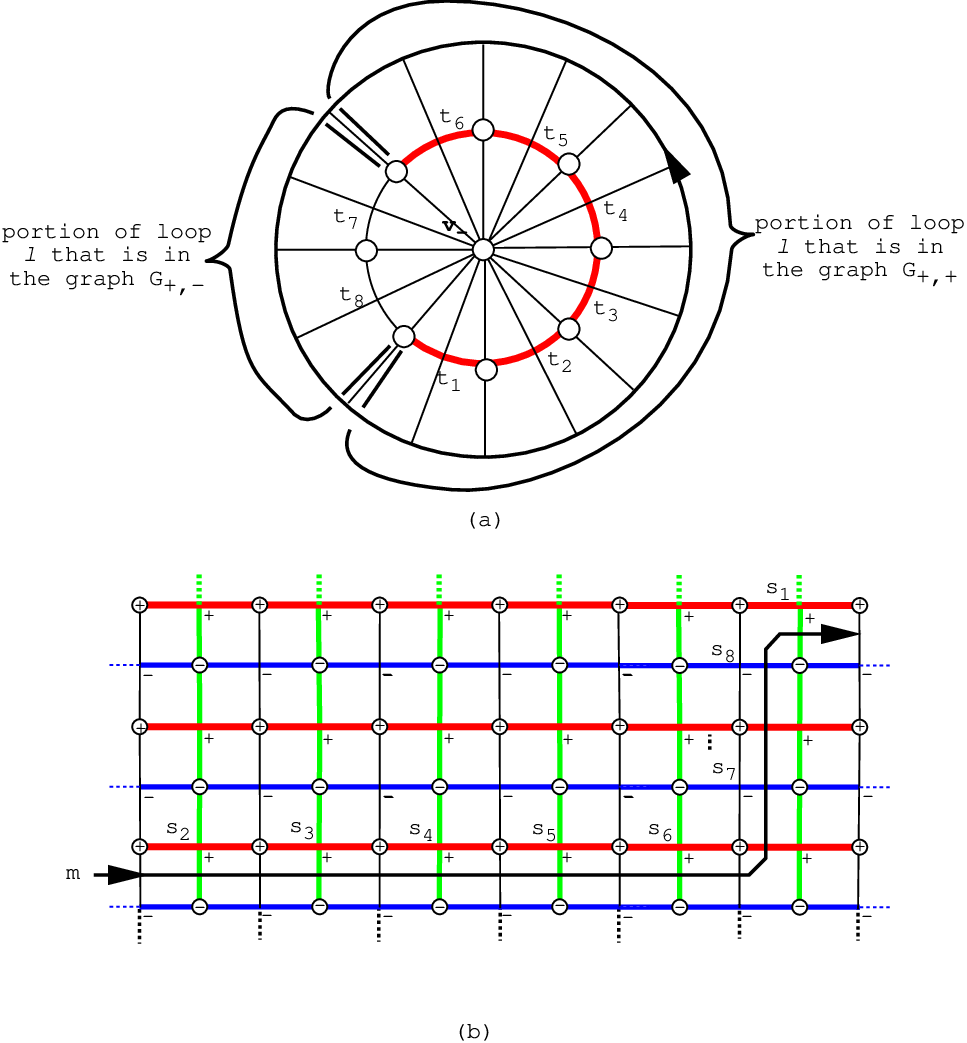
Now consider how the foliations of and are related to one another, when is a parallel push-off of . Let be the annulus in Figure 13 that has and as its boundary curves. Notice that the core circle in that is contained in a union of all of the singular leaves in the induced foliation of is a union of sub-arcs of the graphs . Similar in flavor to the arguments in Proposition 5.8, we can produce a sequence of exchange moves by applying Lemma 5.3 so that either contains no corners, or each component of contains exactly one inside corner and one outside corner. If contains no corners then the foliation of will have singularities all of the same parity. If each component of has exactly one inside and outside corner then the core circle in is the union of an arc in and an arc in .
Now the foliation of is simply the foliation of . Specifically, for each singularity in there is a singularity (coming from the “ portion” of ) that is in a regular neighborhood of on the negative side of the oriented . It is easily checked by appealing to the –sequence of that if is a positive (negative) singularity then is the singularity that occurs immediately before (after) . (See Figure 14.) If contains no corners then the of contains a loop—the core circle coming from . But by Lemma 3.8 of [BF] such a loop cannot exist. So we are left having containing a loop (which is the core circle of ) that is the union of an arc in the graph and an arc in the graph . This loop contains all of the positive vertices of . As noted above, a singularity will in sequentially correspond to a singularity . An application of the argument in Lemma 3.8 (ii) allows us to conclude this discussion of the foliation of with the following summarizing result.
Lemma 5.11.
Let be a quadruple where the triple satisfies the conclusions of Propositions 5.5, 5.8, 5.9 and 5.10. We can assume that the initial foliation of satisfies the following conditions.
- (a)
There are only –singularities.
- (b)
There exists a closed loop that is the union of an arc in and an arc in .
- (c)
When , there is a single negative vertex . When , there is a negative vertex adjacent to two singularities of common parity that are consecutive on .
Moreover, the singularities contained in each component of are in one-to-one correspondence with, and in sequentially correspond to, the singularities contained in . (See Figure 14.)
We now use this initial tiling of to reduce the complexity of the quadruple . Notice that the number of singularities in the loop is naturally two or greater. The next lemma shows us that when contains exactly two singularities the foliation of a tiled must have an inessential –arc.
Lemma 5.12.
Proof.
If then must have contained one positive and one negative singularity. Thus, referring to the terminology of [BM3], must be a type k torus. A type k torus embedding has the property that a meridian curve on can be represented by the union of two –arcs, each being outermost in a disc fiber of . Since can only intersect one of these two –arcs, must contain an inessential –arc. (Refer back to Remark 3.2 and Figure 7 for an example of a type k torus.) ∎
We next deal with the case where contains more than two singularities.
Lemma 5.13.
 \nocolon
Proof.
If then we employ the negative vertex in condition (c) of Lemma 5.11. Figure 15(a) illustrates this situation when the parity of these two singularities is positive. In Figure 15(a) these singularities are labeled and . The common positive vertex that is adjacent to both of their associated singular leaves is . A regular neighborhood of the portion of that contains endpoints of –arcs adjacent to is labeled . If we look at the image of in the foliation of we see that intersects a positive singular leaf containing the singular point associated to ; then a negative singular leaf; then another positive singular leaf containing the singular point associated to . In the –sequence of we know by the discussion in the proof of Lemma 5.11 that occurs immediately before and occurs immediately before .
By Proposition 5.10, there are now three possibilities for the arc : (1) ; (2) intersects the singular leaf belonging to first, then the negative singular leaf and then ; or (3) intersects the singular leaf belonging to first, then intersects some number of times, and then intersects the negative singular leaf.
If (3) occurs we replace with , altering so that its foliation again satisfies the initial condition foliation of Lemma 5.11. This produces a new which corresponds to possibility (2). Now notice in the situation of (2) we can isotopy in so that intersects between the time crosses the singular leaf and the time it crosses the singular leaf. Thus, we can assume that .
 \nocolon
Since and are of the same parity and adjacent to the unique negative vertex in , we can perform a change of foliation. (This is an application to the foliation of of the alteration in Figure 5.) Figure 16(a) show how this change of foliation results in a type (a) vertex, , which locally has the same foliation as that in Figure 3. The boundary of this valence vertex contains . (See Figure 16(a).) We now destabilize through this valence vertex and, since , we can drag along through this destabilization of without altering the embedding of . Figure 16(b) illustrates how the foliation of is altered by this destabilization of . Notice that two new vertices are introduced into the foliation of , one positive and one negative, and that both of these new vertices are valence . We can now appeal to Figure 6 to eliminate four vertices of . This reduces and, thus, the complexity of our quadruple.
Finally, it should be noted that we have made a choice of the parity of for reasons having to do with the clarity of the expository. This does not reduce the generality of the argument. ∎
References
- [1]
- [BF] J Birman, E Finkelstein, Studying surfaces via closed braids, Journal of Knot Theory and its Ramifications, 7 (1998) 267–334
- [BM1] J Birman, W Menasco, Studying Links via Closed Braids V: Closed braid representations of the unlink, Transactions of the AMS, 329 (1992) 585–606
- [BM2] J Birman, W Menasco, Studying Links via Closed Braids IV: Split links and composite links, Inventiones Mathematicae, 102 (1990) 115–139
- [BM3] J Birman, W Menasco, Special positions for essential tori in link complements, Topology, 33 (1994) 525–556
- [BM4] J Birman, W Menasco, Studying Links via Closed Braids IV: Closed links which are –braids, Pacific Journal of Mathematics, 161 (1993) 25–113
- [BW] J Birman, N C Wrinkle, On transversally simple knots, preprint (1999)
- [El] Y Eliashberg, Legendrian and transversal knots in tight contact –manifolds, Topological Methods in Modern Mathematics, (1991) 171–193
- [Et] J Etnyre, Transversal torus knots, Geometry and Topology, 3 (1999) 253–268
- [J] W Jaco, Lectures on Three–Manifold Topology, AMS Regional conference series, No. 43
- [L] J Los, Knots, braid index and dynamical type, Topology, 33 (1994) 257–270
- [R] D Rolfsen, Knots and Links, Mathematics Lecture Series 7, Publish or Perish, Inc. (1976)
- [Sch] H Schubert, Knoten und Vollringe, Acta Math. 90 (1953) 131–226