On the combinatorics of Forrester-Baxter modelsThanks: Research supported by the Australian Research Council (ARC)

Omar Foda and Trevor A. Welsh Thanks: foda@maths.mu.oz.au Thanks: trevor@maths.mu.oz.au Affiliation: Department of Mathematics and Statistics, Affiliation: The University of Melbourne, Victoria, Australia.

Abstract

We provide further boson-fermion $q$ -polynomial identities for the ‘finitised’ Virasoro characters $\chi^{p,p^{\prime}}_{r,s}$ of the Forrester-Baxter minimal models $M(p,p^{\prime})$ , for certain values of $r$ and $s$ . The construction is based on a detailed analysis of the combinatorics of the set ${\mathcal{P}}^{p,p^{\prime}}_{a,b,c}(L)$ of $q$ -weighted, length- $L$ Forrester-Baxter paths, whose generating function $\chi^{p,p^{\prime}}_{a,b,c}(L)$ provides a finitisation of $\chi^{p,p^{\prime}}_{r,s}$ . In this paper, we restrict our attention to the case where the startpoint $a$ and endpoint $b$ of each path both belong to the set of ‘Takahashi lengths’. In the limit $L\to\infty$ , these polynomial identities reduce to $q$ -series identities for the corresponding characters.

We obtain two closely related fermionic polynomial forms for each (finitised) character. The first of these forms uses the classical definition of the Gaussian polynomials, and includes a term that is a (finitised) character of a certain $M(\hat{p},\hat{p}^{\prime})$ where $\hat{p}^{\prime}<p^{\prime}$ . We provide a combinatorial interpretation for this form using the concept of ‘particles’. The second form, which was first obtained using different methods by the Stony-Brook group, requires a modified definition of the Gaussian polynomials, and its combinatorial interpretation requires not only the concept of particles, but also the additional concept of ‘particle annihilation’.

0 Introduction

0.1 Motivation

The physical spectrum of exactly-solvable lattice models can be described in the language of highest-weight infinite dimensional representations of affine and Virasoro algebras [16]. The characters of these representations are $q$ -series that contain detailed information on the structure and symmetries of the corresponding models. In the following discussion, we wish to restrict attention to the characters of Virasoro highest-weight representations.

The earliest known expressions for these characters are due to Feigen and Fuchs [9] and Rocha-Caridi [17]. These expressions have alternating-signs. A number of years ago, the Stony Brook group discovered completely new expressions for the character formulae²² 2 For references to the original Stony Brook papers, please refer to [6].. These expressions have constant-signs³³ 3 The characterisation of the different expressions of the characters as ‘alternating-sign’ and ‘constant-sign’ $q$ -series is valid only for Virasoro but not for affine characters..

For physical reasons that are beyond the scope of this work, the original alternating-sign expressions are also known as ‘bosonic characters’. Correspondingly, the constant-sign expressions are also known as ‘fermionic characters’ ⁴⁴ 4 For a complete discussion of the physical motivation of the terms ‘bosonic’ and ‘fermionic’, please refer to the original literature on the subject as cited in [6]..

The structure of these new character formulae hints at the presence of a completely new formulation of exactly-solvable models⁵⁵ 5 Analogous developments in the context of highest-weight representations of affine algebras also took place. They are outside the scope of this work.. This possibility has attracted attention for a number of reasons. One of these reasons is the fact that certain physical problems, such as the long-distance asymptotics of the correlation functions, are too difficult to handle in the current formulation. Further, there are reasons to believe that the new formulation could be the right starting point to tackle them (see [6] and references therein). At a more technical level, the availability of two distinct formulations is mathematically enriching, as we can use one to learn about the other.

However, although the bosonic characters are technically simple to write down, and are completely known for all Virasoro representations, the structure of the fermionic characters is strictly-speaking known explicitly only in special cases, and generally only conceptually. In particular, the characters of the ‘non-unitary’ Virasoro representations have turned out to be rather resistant to a complete formulation in fermionic form⁶⁶ 6 The reason for that may of course eventually turn out to be the fact that we are not using the most efficient tools to tackle this problem..

This work is part of a series of papers that aim at a complete and explicit derivation of the fermionic characters of a certain class of models first discussed by Forrester and Baxter [14]. The characters of the Forrester-Baxter models correspond to the complete set of Virasoro characters of the discrete, though not necessarily unitary, Virasoro algebras with central charge $c<1$ , first discussed in [4]. As such, they form the largest class of Virasoro characters with no $W$ -symmetries.

As in previous works, our approach is purely combinatorial. Further, the exposition is self-contained, in the sense that we have included all concepts required in the derivations. Our main result is a combinatorial derivation of two related finitised fermionic forms for the characters of a certain class of Forrester-Baxter models. The first of these requires the use of the classical form of Gaussian polynomials and can be interpreted combinatorially using the concept of particles. The second has already appeared in the works of Berkovich, McCoy and Schilling [7], requires the use of a modified form of Gaussian polynomials, and has a combinatorial interpretation in terms of particles and particle annihilation.

In a forthcoming paper, we further extend and refine the techniques of this work to obtain a complete and explicit derivation of the fermionic characters of the complete set of Forrester-Baxter models [13].

0.2 Overview of content of paper

The aim of this paper is to obtain fermionic expressions for ${\chi}^{p,p^{\prime}}_{a,b,c}(L)$ , the generating function for the set ${\mathcal{P}}^{p,p^{\prime}}_{a,b,c}(L)$ of restricted length- $L$ paths that have startpoint $a$ and endpoint $b$ .

These functions⁷⁷ 7 To be precise, a certain renormalisation thereof. first arose in the calculation of one-point functions of the Forrester-Baxter models [14]. The weighting originally assigned in [14] to the paths is significantly different from that used here. The weighting described in the current paper arose by obtaining a ‘weight-preserving’ bijection between partitions with prescribed hook-differences that were considered in [3], and the paths of [14]. This bijection is described in [10].

The paths in ${\mathcal{P}}^{p,p^{\prime}}_{a,b,c}(L)$ may be depicted on a $(p^{\prime}-2)\times L$ grid that we refer to as the $(p,p^{\prime})$ -model, as described in Section 1.1. Of particular importance is the shading of the $(p,p^{\prime})$ -model, which determines the weights ${wt}(h)$ that we assign to the paths $h$ .

A bosonic expression for ${\chi}^{p,p^{\prime}}_{a,b,c}(L)$ is given in Section 1.3. This expression is readily proved using $L$ -recurrence relations [14], or by using the generating function for partitions with prescribed hook-differences given in [3], and the bijection of [10]. The polynomial ${\chi}^{p,p^{\prime}}_{a,b,c}(L)$ is seen to be a finitisation of a Virasoro character.

In this paper, we tackle the particular cases where $a$ and $b$ are each one of the Takahashi lengths $\mathcal{T}$ , or one of $\mathcal{T}^{\prime}=\{p^{\prime}-s:s\in\mathcal{T}\}$ . These values depend on $p$ and $p^{\prime}$ , and are defined in Section 5.1. Our methods and results are a common generalisation of those of [10, 12].

On equating the bosonic expression for ${\chi}^{p,p^{\prime}}_{a,b,c}(L)$ with either of the fermionic expressions, we obtain boson-fermion polynomial identities. Taking the $L\to\infty$ limit (using, for example, the variable change employed in [10, 11]), these become $q$ -series identities. Amongst them, in particular, are the Rogers-Ramanujan identities, and their generalisations by Andrews and Gordon [2]. In fact, the techniques employed by Agarwal and Bressoud [1, 8] in their combinatorial proof of the Andrews-Gordon identities provided the genesis of the techniques employed here.

Before we develop a generalisation of Agarwal and Bressoud’s ‘Volcanic activity’, we define in Section 2, a slightly different set ${\mathcal{P}}^{p,p^{\prime}}_{a,b,e,f}(L)$ of paths, which have assigned pre-segments and post-segments that are determined by $e,f\in\{0,1\}$ . Their generating function $\tilde{\chi}^{p,p^{\prime}}_{a,b,e,f}(L)$ is defined in terms of a path weighting that differs slightly from that defined earlier.

The ${\mathcal{B}}$ -transform, which is described in Section 3, enables $\tilde{\chi}^{p,p^{\prime}+p}_{a^{\prime},b^{\prime},e,f}(L^{\prime})$ , for certain $a^{\prime},b^{\prime}$ to be expressed in terms of $\tilde{\chi}^{p,p^{\prime}+p}_{a,b,e,f}(L)$ . We derive this transform combinatorially in three steps. The first step is known as the ${\mathcal{B}}_{1}$ -transform and enlarges the features of a path, so that the resultant path resides in a larger model. The second step, referred to as a ${\mathcal{B}}_{2}(k)$ -transform, lengthens a path by appending $k$ pairs of segments to the path. Each of these pairs is known as a particle. The third step, the ${\mathcal{B}}_{3}(\lambda)$ -transform deforms the path in a particular way. This process may be viewed as the particles moving through the path. The resulting transformation of generating functions is given in Corollary 3.14.

In Section 4, we see that $\tilde{\chi}^{p^{\prime}-p,p^{\prime}}_{a,b,1-e,1-f}(L)$ may be obtained from $\tilde{\chi}^{p,p^{\prime}}_{a,b,e,f}(L)$ in a combinatorially trivial way. This process is referred to as a ${\mathcal{D}}$ -transform. In fact, it is more convenient to use the ${\mathcal{D}}$ -transform combined with the ${\mathcal{B}}$ -transform. The resulting transformation of generating functions is given in Corollary 4.6.

To obtain a particular generating function $\tilde{\chi}^{p,p^{\prime}}_{a,b,e,f}(L)$ , where $p$ and $p^{\prime}$ are co-prime, we begin with one of the trivial generating functions $\tilde{\chi}^{1,3}_{a^{\prime},b^{\prime},e^{\prime},f^{\prime}}(L)$ given in Lemma 2.5, and perform a sequence of ${\mathcal{B}}$ - and ${\mathcal{B}}{\mathcal{D}}$ -transforms. This sequence is determined by the continued fraction of $p^{\prime}/p$ which is described in Section 5.1.

In fact, a basic application of the transforms does not generate all elements of ${\mathcal{P}}^{p,p^{\prime}}_{a,b,e,f}(L)$ in some cases. In these instances, the set generated is deficient in the full set of paths that do not rise above (or below) a certain height. Various results obtained in Section 6 enable us to keep track of this height. Lemma 6.4 shows that this height bounds a portion of the $(p,p^{\prime})$ -model which is identical to a smaller $(\hat{p},\hat{p}^{\prime})$ -model. This property enables (in one case), the final generating function to be expressed using the generating function for paths in the $(\hat{p},\hat{p}^{\prime})$ -model.

Section 7 provides one further ingredient for the final construction. There, it is shown how appending or removing the first segment of the path affects the generating function.

Everything is now in place to carry out the proof of the main results. These results are stated in Section 8.1. We provide two similar expressions for ${\chi}^{p,p^{\prime}}_{a,b,c}(L)$ . These are Theorems 8.1 and 8.2. The first of these makes use of the classical definition of the Gaussian polynomial:

\left[{A\atop B}\right]_{q}=\left\{\begin{array}[]{cl}\frac{\displaystyle(q)_{A}}{\displaystyle(q)_{A-B}(q)_{B}}&\quad\mbox{if }0\leq B\leq A;\\[8.53581pt] 0&\quad\mbox{otherwise},\end{array}\right.

(1)

where $(q)_{0}=1$ and $(q)_{n}=\prod_{i=1}^{n}(1-q^{i})$ for $n>0$ . In some cases, the expression also includes a term ${\chi}^{\hat{p},\hat{p}^{\prime}}_{a,b,c}(L)$ for $\hat{p}^{\prime}<\hat{p}$ . Thus this expression may be viewed as a recursive fermionic expression for ${\chi}^{p,p^{\prime}}_{a,b,c}(L)$ . In the cases where this additional term is not present (for $a$ and $b$ further restricted in a certain way), the expressions were first stated in [5].

The expression of Theorem 8.2 makes use of a modified definition of the Gaussian polynomial ([15]):

\left[{A\atop B}\right]^{\prime}_{q}=\left\{\begin{array}[]{cl}\frac{\displaystyle(q^{A-B+1})_{B}}{\displaystyle(q)_{B}}&\quad\mbox{if }0\leq B;\\[8.53581pt] 0&\quad\mbox{otherwise},\end{array}\right.

(2)

where $(z)_{0}=1$ and $(z)_{n}=\prod_{i=0}^{n-1}(1-zq^{i})$ for $n>0$ . These expressions were first presented and proved in [7]. In fact, invoking the definition (2) is somewhat overkill, since the only value of $\left[{A\atop B}\right]^{\prime}$ that we require that differs from $\left[{A\atop B}\right]$ is $\left[{-1\atop 0}\hbox to0.0pt{$\phantom{A\atop B}$\hss}\right]^{\prime}=1$ .

In [7], expressions for ${\chi}^{p,p^{\prime}}_{a,b,c}(L)$ are presented, where $b$ is now any value with $1\leq b\leq p^{\prime}-1$ . However, only $a\in\mathcal{T}\cup\mathcal{T}^{\prime}$ is still permitted. In [13], we show that it is Theorem 8.1, and not Theorem 8.2, that generalises to provide fermionic expressions for the most general ${\chi}^{p,p^{\prime}}_{a,b,c}(L)$ .

The remainder of Section 8 is concerned with the detailed derivation of the expression for first $\tilde{\chi}^{p,p^{\prime}}_{a,b,e,f}(L)$ , and then converting it to ${\chi}^{p,p^{\prime}}_{a,b,c}(L)$ . Section 8.3 describes the $m$ $n$ -system which aids the actual evaluation of the fermionic expressions obtained. Section 8.4 describes how the proof for Theorem 8.1 modifies to provide a proof for Theorem 8.2. Here we see that the appearance of $\left[{-1\atop 0}\hbox to0.0pt{$\phantom{A\atop B}$\hss}\right]^{\prime}$ may be viewed in terms of ‘particle annihilation’.

1 Paths

1.1 Paths and the $(p,p^{\prime})$ -model

Let $p$ and $p^{\prime}$ be positive co-prime integers for which $0<p<p^{\prime}$ . Then, given $a,b,c,L\in{\tensym Z}_{\geq 0}$ such that $1\leq a,b,c\leq p^{\prime}-1$ , $b=c\pm 1$ , $L+a-b\equiv 0$ ( $\mbox{mod}\,2$ ), a path $h\in{\mathcal{P}}^{p,p^{\prime}}_{a,b,c}(L)$ is a sequence $h_{0},h_{1},h_{2},\ldots,h_{L},$ of integers such that:

1.

$1\leq h_{i}\leq p^{\prime}-1$ for $0\leq i\leq L$ ,
2.

$h_{i+1}=h_{i}\pm 1$ for $0\leq i<L$ ,
3.

$h_{0}=a,h_{L}=b.$

Note that the values of $p$ and $c$ do not feature in the above restrictions. As described below, they specify how the elements of ${\mathcal{P}}^{p,p^{\prime}}_{a,b,c}(L)$ are weighted.

The integers $h_{0},h_{1},h_{2},\ldots,h_{L},$ are readily depicted as a sequence of heights on a two-dimensional $L\times(p^{\prime}-2)$ grid. Adjacent heights are connected by line segments passing from $(i,h_{i})$ to $(i+1,h_{i+1})$ for $0\leq i<L$ .

Scanning the path from left to right, each of these line segments points either in the NE direction or in the SE direction. Fig. 1 shows a typical path in the set ${\mathcal{P}}^{3,8}_{2,4,3}(14)$ . The shadings in Fig. 1 are explained below.

Refer to caption — Figure 1: Typical path.

In the grid introduced above, the horizontal strip between adjacent heights is referred to as a band. There are $p^{\prime}-2$ bands. The $h$ th band lies between heights $h$ and $h+1$ .

We now assign a parity to each band: the $h$ th band is said to be an even band if $\lfloor hp/p^{\prime}\rfloor=\lfloor(h+1)p/p^{\prime}\rfloor$ ; and an odd band if $\lfloor hp/p^{\prime}\rfloor\neq\lfloor(h+1)p/p^{\prime}\rfloor$ . The array of odd and even bands so obtained will be referred to as the $(p,p^{\prime})$ -model. It may immediately be deduced that the $(p,p^{\prime})$ -model has $p^{\prime}-p-1$ even bands and $p-1$ odd bands. In addition, it is easily shown that for $1\leq r<p$ , the band lying between heights $\lfloor rp^{\prime}/p\rfloor$ and $\lfloor rp^{\prime}/p\rfloor+1$ is odd: it will be referred to as the $r$ th odd band.

When drawing the $(p,p^{\prime})$ -model, we distinguish the bands by shading the odd bands. This was done in Fig. 1 for the $(3,8)$ -model.

We note that the band structure of the $(p,p^{\prime})$ -model is up-down symmetrical, and that if $p^{\prime}>2p$ then the 1st band and the $(p^{\prime}-2)$ th band are both even, and there are no two adjacent odd bands.

For $2\leq a\leq p^{\prime}-2$ , we say that $a$ is interfacial if $\lfloor(a+1)p/p^{\prime}\rfloor=\lfloor(a-1)p/p^{\prime}\rfloor+1$ . Thus $a$ is interfacial if and only if $a$ lies between an odd and even band in the $(p,p^{\prime})$ -model. Thus for the case of the $(3,8)$ -model depicted in Fig. 1, $a$ is interfacial for $a=2,3,5,6$ . Note that if $a$ is interfacial, the odd band that it borders is the $\lfloor(a+1)p/p^{\prime}\rfloor$ th.

As is easily seen, the $(p^{\prime}-p,p^{\prime})$ -model differs from the $(p,p^{\prime})$ -model in that each band has changed parity. It follows that if $a$ is interfacial in the $(p,p^{\prime})$ -model then $a$ is also interfacial in the $(p^{\prime}-p,p^{\prime})$ -model.

1.2 Weighting the paths

Given a path $h$ of length $L$ , for $1\leq i<L$ , the values of $h_{i-1}$ , $h_{i}$ and $h_{i+1}$ determine the shape of the vertex at the point $i$ . The four possible shapes are given in Fig. 2.

The four types of vertices shown in Fig. 2 are referred to as a straight-up vertex, a straight-down vertex, a peak-up vertex and a peak-down vertex respectively. Each vertex is also assigned a parity: this is the parity of the band in which the segment between $(i,h_{i})$ and $(i+1,h_{i+1})$ lies. Thus, there are eight types of paritied vertex.

For paths $h\in{{\mathcal{P}}}^{p,p^{\prime}}_{a,b,c}(L)$ , we define $h_{L+1}=c$ , whereupon the shape and parity of the vertex at $i=L$ is well-defined.

The weight function for the paths is best specified in terms of a $(x,y)$ -coordinate system which is inclined at $45^{o}$ to the original $(i,h)$ -coordinate system and whose origin is at the path’s initial point at $(i=0,h=a)$ . Specifically,

x={{i-(h-a)}\over{2}},\qquad y={{i+(h-a)}\over{2}}.

Note that at each step in the path, either $x$ or $y$ is incremented and the other is constant. In this system, the path depicted in Fig. 1 has its first few coordinates at $(0,0)$ , $(0,1)$ , $(0,2)$ , $(0,3)$ , $(1,3)$ , $(1,4)$ , $(1,5)$ , $(1,6)$ , $(2,6)$ , $\ldots$

Now, for $1\leq i\leq L$ , we define the weight $c_{i}=c(h_{i-1},h_{i},h_{i+1})$ of the $i$ th vertex according to its shape, its parity and its $(x,y)$ -coordinate, as specified in Table 1.

Vertex	${c}_{i}$	Vertex	${c}_{i}$
	$x$		$0$
	$y$		$0$
	$0$		$x$
	$0$		$y$

Table 1: Vertex weights.

In Table 1, the lightly shaded bands can be either even or odd bands (or when $h_{i}=p^{\prime}-1$ or $h_{i}=1$ in the lowermost four cases, not a band in the model at all). Note that for each vertex shape, only one parity case has non-zero weight in general. We shall refer to those four vertices, with assigned parity, for which in general, the weight is non-zero, as scoring vertices. The other four vertices will be termed non-scoring.

We now define:

{wt}(h)=\sum_{i=1}^{L}c_{i}.

(3)

To illustrate this procedure, consider again the path $h$ depicted in Fig. 1. The above table indicates that there are scoring vertices at $i=3$ , $4$ , $5$ , $7$ , $8$ , $13$ and $14$ . This leads to

{wt}(h)=0+3+1+1+6+7+6=24.

The generating function ${\chi}^{p,p^{\prime}}_{a,b,c}(L)$ for the set of paths ${{\mathcal{P}}}^{p,p^{\prime}}_{a,b,c}(L)$ is defined to be:

{\chi}^{p,p^{\prime}}_{a,b,c}(L;q)=\sum_{h\in{{\mathcal{P}}}^{p,p^{\prime}}_{a,b,c}(L)}q^{{wt}(h)}.

(4)

Often, we drop the base $q$ from the notation so that ${\chi}^{p,p^{\prime}}_{a,b,c}(L)={\chi}^{p,p^{\prime}}_{a,b,c}(L;q)$ . The same will be done for other functions without comment.

1.3 Bosonic generating function

By setting up recurrence relations for ${\chi}^{p,p^{\prime}}_{a,b,c}(L)$ , it may be readily verified that:

	$\displaystyle\chi^{p,p^{\prime}}_{a,b,c}(L)$	$\displaystyle=$	$\displaystyle\sum_{\lambda=-{\infty}}^{\infty}q^{\lambda^{2}pp^{\prime}+\lambda(p^{\prime}r-pa)}\left[{L\atop{\frac{L+a-b}{2}}-p^{\prime}\lambda}\right]_{q}$		(5)
			$\displaystyle\qquad\qquad\qquad-\sum_{\lambda=-\infty}^{\infty}q^{(\lambda p+r)(\lambda p^{\prime}+a)}\left[{L\atop{\frac{L+a-b}{2}}-p^{\prime}\lambda-a}\right]_{q},$		(5)

where

r=\lfloor pc/p^{\prime}\rfloor+(b-c+1)/2.

(6)

In the limit $L\mapsto\infty$ , we obtain

\lim_{L\to\infty}\chi^{p,p^{\prime}}_{a,b,c}(L)=\chi^{p,p^{\prime}}_{r,a},

(7)

where $r$ is defined in (6) and

\chi^{p,p^{\prime}}_{r,s}={\frac{1}{(q)_{\infty}}}\sum_{\lambda=-\infty}^{\infty}(q^{\lambda^{2}pp^{\prime}+\lambda(p^{\prime}r-ps)}-q^{(\lambda p+r)(\lambda p^{\prime}+s)})

(8)

is, up to a normalisation, the Rocha-Caridi expression [17] for the Virasoro character of central charge $c=1-{6(p^{\prime}-p)^{2}}/{pp^{\prime}}$ and conformal dimension $\Delta^{p,p^{\prime}}_{r,s}={\left((p^{\prime}r-ps)^{2}-(p^{\prime}-p)^{2}\right)}/{4pp^{\prime}}$ . Therefore, $\chi^{p,p^{\prime}}_{a,b,c}(L)$ provides a finite analogue of the character $\chi^{p,p^{\prime}}_{r,a}$ .

2 Winged generating functions

For $h\in{\mathcal{P}}^{p,p^{\prime}}_{a,b,c}(L)$ , the values of $b$ and $c$ serve to specify a path post-segment that extends between $(L,b)$ and $(L+1,c)$ . We now define another set of paths which specifies both the direction of a post-segment and a pre-segment.

Let $p$ and $p^{\prime}$ be positive co-prime integers for which $0<p<p^{\prime}$ . Then, given $a,b,L\in{\tensym Z}_{\geq 0}$ such that $1\leq a,b\leq p^{\prime}-1$ , $L+a-b\equiv 0$ ( $\mbox{mod}\,2$ ), and $e,f\in\{0,1\}$ , a path $h\in{\mathcal{P}}^{p,p^{\prime}}_{a,b,e,f}(L)$ is a sequence $h_{0},h_{1},h_{2},\ldots,h_{L},$ of integers such that:

1.

$1\leq h_{i}\leq p^{\prime}-1$ for $0\leq i\leq L$ ,
2.

$h_{i+1}=h_{i}\pm 1$ for $0\leq i<L$ ,
3.

$h_{0}=a,h_{L}=b.$

If $f=0$ (resp. $f=1$ ) then the post-segment of each $h\in{\mathcal{P}}^{p,p^{\prime}}_{a,b,e,f}(L)$ is defined to be in the NE (resp. SE) direction. If $e=0$ (resp. $e=1$ ) then the pre-segment of each $h\in{\mathcal{P}}^{p,p^{\prime}}_{a,b,e,f}(L)$ is defined to be in the SE (resp. NE) direction. This enables a shape and a parity to be assigned to both the zeroth and the $L$ th vertices of $h$ . For $h\in{\mathcal{P}}^{p,p^{\prime}}_{a,b,e,f}(L)$ , we define $e(h)=e$ and $f(h)=f$ .

We now define a weight $\tilde{wt}(h)$ , for $h\in{\mathcal{P}}^{p,p^{\prime}}_{a,b,e,f}(L)$ . For $1\leq i<L$ , set $\tilde{c}_{i}=c(h_{i-1},h_{i},h_{i+1})$ as above. Then, set

\tilde{c}_{L}=\left\{\begin{array}[]{ll}x&\mbox{if }h_{L}-h_{L-1}=\phantom{-}1\mbox{ and }f(h)=1;\\[4.2679pt] y&\mbox{if }h_{L}-h_{L-1}=-1\mbox{ and }f(h)=0;\\[4.2679pt] 0&\mbox{otherwise,}\end{array}\right.

where $(x,y)$ is the coordinate of the $L$ th vertex of $h$ . We then designate this vertex as scoring if it is a peak vertex ( $h_{L}=h_{L-1}-(-1)^{f(h)}$ ), and as non-scoring otherwise.

We define:

\tilde{wt}(h)=\sum_{i=1}^{L}\tilde{c}_{i}.

(9)

Consider the corresponding path $h^{\prime}\in{\mathcal{P}}^{p,p^{\prime}}_{a,b,c}(L)$ with $c=b+(-1)^{f}$ , defined by $h_{i}^{\prime}=h_{i}$ for $0\leq i\leq L$ . From Table 1, we see that $\tilde{wt}(h)={wt}(h^{\prime})$ if the post-segment of $h$ lies in an even band.

In what follows, we work entirely in terms of $\tilde{wt}(h)$ , and the generating functions that we derive from it. Only at the end of our work, do we revert back to ${wt}(h)$ to obtain fermionic expressions for ${\chi}^{p,p^{\prime}}_{a,b,c}(L)$ .

Define the generating function

\tilde{\chi}^{p,p^{\prime}}_{a,b,e,f}(L;q)=\sum_{h\in{{\mathcal{P}}}^{p,p^{\prime}}_{a,b,e,f}(L)}q^{\tilde{wt}(h)},

(10)

where $\tilde{wt}(h)$ is given by (9). Of course, $\tilde{\chi}^{p,p^{\prime}}_{a,b,0,f}(L)=\tilde{\chi}^{p,p^{\prime}}_{a,b,1,f}(L)$ .

2.1 Striking sequence of a path

For each path $h$ , define $\pi(h)\in\{0,1\}$ to be the parity of the band between heights $h_{0}$ and $h_{1}$ (if $L(h)=0$ , we set $h_{1}=h_{0}+(-1)^{f(h)}$ ). Thus, for the path $h$ shown in Fig. 1, we have $\pi(h)=1$ . In addition, define $d(h)=0$ when $h_{1}-h_{0}=1$ and $d(h)=1$ when $h_{1}-h_{0}=-1$ . We then see that if $e(h)+d(h)+\pi(h)\equiv 0\,(\mbox{mod}\,2)$ then the $0$ th vertex is a scoring vertex, and if $e(h)+d(h)+\pi(h)\equiv 1\,(\mbox{mod}\,2)$ then it is a non-scoring vertex.

Now consider each path $h\in{{\mathcal{P}}}^{p,p^{\prime}}_{a,b,e,f}(L)$ as a sequence of straight lines, alternating in direction between NE and SE. Then, reading from the left, let the lines be of lengths $w_{1}$ , $w_{2}$ , $w_{3},\ldots,w_{l},$ for some $l$ , with $w_{i}>0$ for $1\leq i\leq l$ . Thence $w_{1}+w_{2}+\cdots+w_{l}=L(h)$ , where $L(h)=L$ is the length of $h$ .

For each of these lines, the last vertex will be considered to be part of the line but the first will not. Then, the $i$ th of these lines contains $w_{i}$ vertices, the first $w_{i}-1$ of which are straight vertices. Then write $w_{i}=a_{i}+b_{i}$ so that $b_{i}$ is the number of scoring vertices in the $i$ th line. The striking sequence of $h$ is then the array:

\left(\begin{array}[]{ccccc}a_{1}&a_{2}&a_{3}&\cdots&a_{l}\\ b_{1}&b_{2}&b_{3}&\cdots&b_{l}\end{array}\right)^{(e(h),f(h),d(h))}.

With $\pi=\pi(h)$ , $e=e(h)$ and $d=d(h)$ , we define

m(h)=\left\{\begin{array}[]{ll}(e+d+\pi)\,\mbox{mod}\,2+\sum_{i=1}^{l}a_{i}&\mbox{if }L>0;\\[4.2679pt] |f-e|&\mbox{if }L=0,\end{array}\right.

whence $m(h)$ is the number of non-scoring vertices possessed by $h$ (altogether, $h$ has $L(h)+1$ vertices). We also define $\alpha(h)=(-1)^{d}((w_{1}+w_{3}+\cdots)-(w_{2}+w_{4}+\cdots))$ and for $L>0$ ,

\beta(h)=\left\{\begin{array}[]{l}(-1)^{d}((b_{1}+b_{3}+\cdots)-(b_{2}+b_{4}+\cdots))\\ \hskip 113.81102pt\mbox{if }e+d+\pi\equiv 0\,(\mbox{mod}\,2);\\[4.2679pt] (-1)^{d}((b_{1}+b_{3}+\cdots)-(b_{2}+b_{4}+\cdots))+(-1)^{e}\\ \hskip 113.81102pt\mbox{otherwise.}\end{array}\right.

For $L=0$ , we set $\beta(h)=f-e$ .

For example, for the path shown in Fig. 1 for which $d(h)=0$ and $\pi(h)=1$ , the striking sequence is:

\left({2\enskip 0\enskip 1\enskip 1\enskip 1\enskip 2\enskip 0\atop 1\enskip 1\enskip 2\enskip 1\enskip 0\enskip 1\enskip 1}\right)^{(e,1,0)}.

In this case, $m(h)=8-e$ , $\alpha(h)=2$ , and $\beta(h)=2-e$ .

We note that given the startpoint $h_{0}=a$ of the path, the path can be reconstructed from its striking sequence⁸⁸ 8 We only need $w_{1},w_{2},\ldots,w_{l}$ together with $d$ .. In particular, $h_{L}=b=a+\alpha(h)$ . In addition, the nature of the final vertex may be deduced from $a_{l}$ and $b_{l}$ ⁹⁹ 9 Thus the value of $f$ in the striking sequence is redundant — we retain it for convenience.

Lemma 2.1

Let the path $h$ have the striking sequence $\left({a_{1}\atop b_{1}}\,{a_{2}\atop b_{2}}\,{a_{3}\atop b_{3}}\,{\cdots\atop\cdots}\,{a_{l}\atop b_{l}}\right)^{(e,f,d)}\!,$ with $w_{i}=a_{i}+b_{i}$ for $1\leq i\leq l$ . Then

\tilde{wt}(h)=\sum_{i=1}^{l}b_{i}(w_{i-1}+w_{i-3}+\cdots+w_{1+i\bmod 2}).

Proof: For $L=0$ , both sides are clearly $0$ . So assume $L>0$ . First consider $d=0$ . For $i$ odd, the $i$ th line is in the NE direction and its $x$ -coordinate is $w_{2}+w_{4}+\cdots+w_{i-1}$ . By the prescription of the previous section, and the definition of $b_{i}$ , this line thus contributes $b_{i}(w_{2}+w_{4}+\cdots+w_{i-1})$ to the weight $\tilde{wt}(h)$ of $h$ . Similarly, for $i$ even, the $i$ th line is in the SE direction and contributes $b_{i}(w_{1}+w_{3}+\cdots+w_{i-1})$ to $\tilde{wt}(h)$ . The lemma then follows for $d=0$ . The case $d=1$ is similar. $\Box$

2.2 Path parameters

We make the following definitions:

\begin{array}[]{ll}\alpha^{p,p^{\prime}}_{a,b}&=\>b-a;\\[1.42262pt] \beta^{p,p^{\prime}}_{a,b,e,f}&=\>\left\lfloor\frac{bp}{p^{\prime}}\right\rfloor-\left\lfloor\frac{ap}{p^{\prime}}\right\rfloor+f-e;\\[7.11317pt] \delta^{p,p^{\prime}}_{a,e}&=\>\left\{\begin{array}[]{ll}0&\mbox{if }\left\lfloor\frac{(a+(-1)^{e})p}{p^{\prime}}\right\rfloor=\left\lfloor\frac{ap}{p^{\prime}}\right\rfloor;\\[8.53581pt] 1&\mbox{if }\left\lfloor\frac{(a+(-1)^{e})p}{p^{\prime}}\right\rfloor\neq\left\lfloor\frac{ap}{p^{\prime}}\right\rfloor.\end{array}\right.\\ \end{array}

(The superscripts of $\alpha^{p,p^{\prime}}_{a,b}$ are superfluous, of course.) It may be seen that the value of $\delta^{p,p^{\prime}}_{a,e}$ gives the parity of the band in which the path pre-segment resides.

Lemma 2.2

Let $h\in{{\mathcal{P}}}^{p,p^{\prime}}_{a,b,e,f}(L)$ . Then $\alpha(h)=\alpha^{p,p^{\prime}}_{a,b}$ and $\beta(h)=\beta^{p,p^{\prime}}_{a,b,e,f}$ .

Proof: That $\alpha(h)=\alpha^{p,p^{\prime}}_{a,b}$ follows immediately from the definitions.

The second result is proved by induction on $L$ . If $h\in{{\mathcal{P}}}^{p,p^{\prime}}_{a,b,e,f}(0)$ then $a=b$ , whence $\beta^{p,p^{\prime}}_{a,b,e,f}=f-e=\beta(h)$ , immediately from the definitions.

For $L>0$ , let $h\in{{\mathcal{P}}}^{p,p^{\prime}}_{a,b,e,f}(L)$ and assume that the result holds for all $h^{\prime}\in{{\mathcal{P}}}^{p,p^{\prime}}_{a,b^{\prime},e,f^{\prime}}(L-1)$ . We consider a particular $h^{\prime}$ by setting $h_{i}^{\prime}=h_{i}$ for $0\leq i<L$ , $b^{\prime}=h_{L-1}$ and choosing $f^{\prime}\in\{0,1\}$ so that $f^{\prime}=0$ if either $b-b^{\prime}=1$ and the $L$ th segment of $h$ lies in an even band, or $b-b^{\prime}=-1$ and the $L$ th segment of $h$ lies in an odd band; and $f^{\prime}=1$ otherwise. It may easily be checked that the $(L-1)$ th vertex of $h^{\prime}$ is scoring if and only if the $(L-1)$ th vertex of $h$ is scoring. Then, from the definition of $\beta(h)$ , we see that:

\beta(h)=\left\{\begin{array}[]{ll}\beta(h^{\prime})+1&\mbox{if }b-b^{\prime}=\phantom{-}1\mbox{ and }f=1;\\ \beta(h^{\prime})-1&\mbox{if }b-b^{\prime}=-1\mbox{ and }f=0;\\ \beta(h^{\prime})&\mbox{otherwise.}\end{array}\right.

The induction hypothesis gives $\beta(h^{\prime})=\lfloor b^{\prime}p/p^{\prime}\rfloor-\lfloor ap/p^{\prime}\rfloor+f^{\prime}-e$ . Then when the $L$ th segment of $h$ lies in an even band so that $\lfloor bp/p^{\prime}\rfloor=\lfloor b^{\prime}p/p^{\prime}\rfloor$ , consideration of the four cases of $b-b^{\prime}=\pm 1$ and $f\in\{0,1\}$ shows that $\beta(h)=\lfloor bp/p^{\prime}\rfloor-\lfloor ap/p^{\prime}\rfloor+f-e$ . When the $L$ th segment of $h$ lies in an odd band so that $\lfloor bp/p^{\prime}\rfloor=\lfloor b^{\prime}p/p^{\prime}\rfloor+b-b^{\prime}$ , consideration of the four cases of $b-b^{\prime}=\pm 1$ and $f\in\{0,1\}$ again shows that $\beta(h)=\lfloor bp/p^{\prime}\rfloor-\lfloor ap/p^{\prime}\rfloor+f-e$ . The result follows by induction. $\Box$

2.3 Scoring generating functions

We now define a generating function for paths that have a particular number of non-scoring vertices. First define ${{\mathcal{P}}}^{p,p^{\prime}}_{a,b,e,f}(L,m)$ to be the subset of ${{\mathcal{P}}}^{p,p^{\prime}}_{a,b,e,f}(L)$ comprising those paths $h$ for which $m(h)=m$ . Then define:

{\chi}^{p,p^{\prime}}_{a,b,e,f}(L,m;q)=\sum_{h\in{{\mathcal{P}}}^{p,p^{\prime}}_{a,b,e,f}(L,m)}q^{\tilde{wt}(h)}.

(11)

Lemma 2.3

Let $\beta=\beta^{p,p^{\prime}}_{a,b,e,f}$ . Then

{\chi}^{p,p^{\prime}}_{a,b,e,f}(L)=\sum_{\scriptstyle m\equiv L+\beta\atop\scriptstyle(\mbox{\scriptsize\rm mod}\,2)}{\chi}^{p,p^{\prime}}_{a,b,e,f}(L,m).

Proof: Let $h\in{\mathcal{P}}^{p,p^{\prime}}_{a,b,e,f}(L)$ . We claim that $m(h)+L(h)+\beta(h)\equiv 0\,(\mbox{mod}\,2)$ . This will follow from showing that $L(h)-m(h)+(-1)^{d(h)}\beta(h)$ is even. If $h$ has striking sequence $\left({a_{1}\atop b_{1}}\>{a_{2}\atop b_{2}}\>{a_{3}\atop b_{3}}\>{\cdots\atop\cdots}\>{a_{l}\atop b_{l}}\right)^{(e,f,d)},$ then $L(h)-m(h)=(b_{1}+b_{2}+\cdots+b_{l})-(e+d+\pi)\,\mbox{mod}\,2$ , where $\pi=\pi(h)$ . For $e+d+\pi\equiv 0\,(\mbox{mod}\,2)$ , we immediately obtain $L(h)-m(h)+(-1)^{d}\beta(h)=2(b_{1}+b_{3}+\ldots)$ . For $e+d+\pi\not\equiv 0\,(\mbox{mod}\,2)$ , we obtain $L(h)-m(h)+(-1)^{d}\beta(h)=2(b_{1}+b_{3}+\ldots)-1+(-1)^{d+e}$ , whence the claim is proved in all cases. The lemma then follows, once it is noted, via Lemma 2.2, that $\beta(h)=\beta^{p,p^{\prime}}_{a,b,e,f}$ . $\Box$

Note 2.4

Since each element of ${{\mathcal{P}}}^{p,p^{\prime}}_{a,b,e,f}(L,m)$ has $L+1$ vertices, it follows that ${\chi}^{p,p^{\prime}}_{a,b,e,f}(L,m)$ is non-zero only if $0\leq m\leq L+1$ . Therefore the sum in Lemma 2.3 may be further restricted to $0\leq m\leq L+1$ .

2.4 A seed

The following result provides a seed on which the results of later sections will act.

Lemma 2.5

If $L\geq 0$ is even then:

{\chi}^{1,3}_{1,1,0,0}(L,m)={\chi}^{1,3}_{2,2,1,1}(L,m)=\delta_{m,0}q^{\frac{1}{4}L^{2}}.

If $L>0$ is odd then:

{\chi}^{1,3}_{1,2,0,1}(L,m)={\chi}^{1,3}_{2,1,1,0}(L,m)=\delta_{m,0}q^{\frac{1}{4}(L^{2}-1)}.

Proof: The $(1,3)$ -model comprises one even band. Thus when $L$ is even, there is precisely one $h\in{\mathcal{P}}^{1,3}_{1,1,0,0}(L)$ . It has $h_{i}=1$ for $i$ even, and $h_{i}=2$ for $i$ odd. We see that $h$ has striking sequence $\left({0\atop 1}\>{0\atop 1}\>{0\atop 1}\>{\cdots\atop\cdots}\>{0\atop 1}\right)^{(0,0,0)}$ and $m(h)=0$ . Lemma 2.1 then yields $\tilde{wt}(h)=0+1+1+2+2+3+\cdots+(\frac{1}{2}L-1)+\frac{1}{2}L=(L/2)^{2}$ , as required.

The other expressions follow in a similar way. $\Box$

2.5 Partitions

A partition $\lambda=(\lambda_{1},\lambda_{2},\ldots,\lambda_{k})$ is a sequence of $k$ integer parts $\lambda_{1},\lambda_{2},\ldots,\lambda_{k},$ satisfying $\lambda_{1}\geq\lambda_{2}\geq\cdots\geq\lambda_{k}>0$ . It is to be understood that $\lambda_{i}=0$ for $i>k$ . The weight ${\rm wt\,}(\lambda)$ of $\lambda$ is given by ${\rm wt\,}(\lambda)=\sum_{i=1}^{k}\lambda_{i}$ .

We define ${\mathcal{Y}}(k,m)$ to be the set of all partitions $\lambda$ with at most $k$ parts, and for which $\lambda_{1}\leq m$ . A proof of the following well known result may be found in [2].

Lemma 2.6

The generating function,

\sum_{\lambda\in{\mathcal{Y}}(k,m)}q^{{\rm wt\,}(\lambda)}=\left[{m+k\atop m}\right]_{q}.

3 The ${\mathcal{B}}$ -transform

In this section, we introduce the ${\mathcal{B}}$ -transform which maps paths ${{\mathcal{P}}}^{p,p^{\prime}}_{a,b,e,f}(L)$ into ${{\mathcal{P}}}^{p,p^{\prime}+p}_{a^{\prime},b^{\prime},e,f}(L^{\prime})$ for certain $a^{\prime}$ , $b^{\prime}$ and various $L^{\prime}$ .

The band structure of the $(p,p^{\prime}+p)$ -model is easily obtained from that of the $(p,p^{\prime})$ -model. Indeed, according to Section 1.1, for $1\leq r<p$ , the $r$ th odd band of the $(p,p^{\prime}+p)$ -model lies between heights $\lfloor r(p^{\prime}+p)/p\rfloor=\lfloor rp^{\prime}/p\rfloor+r$ and $\lfloor r(p^{\prime}+p)/p\rfloor+1=\lfloor rp^{\prime}/p\rfloor+r+1$ . Thus the height of the $r$ th odd band in the $(p,p^{\prime}+p)$ -model is $r$ greater than that in the $(p,p^{\prime})$ -model. Therefore, the $(p,p^{\prime}+p)$ -model may be obtained from the $(p,p^{\prime})$ -model by increasing the distance between neighbouring odd bands by one unit and appending an extra even band to both the top and the bottom of the grid. For example, compare the $(3,8)$ -model of Fig. 1 with the $(3,11)$ -model of Fig. 3.

The ${\mathcal{B}}$ -transform has three components, which we refer to as path-dilation, particle-insertion, and particle-motion. These three components will also be known as the ${\mathcal{B}}_{1}$ -, ${\mathcal{B}}_{2}$ - and ${\mathcal{B}}_{3}$ -transforms respectively. In fact, particle-insertion is dependent on a parameter $k\in{\tensym Z}_{\geq 0}$ , and particle-motion is dependent on a partition $\lambda$ that has certain restrictions. Consequently, we sometimes refer to particle-insertion and particle-motion as ${\mathcal{B}}_{2}(k)$ - and ${\mathcal{B}}_{3}(\lambda)$ -transforms respectively. Then, combining the ${\mathcal{B}}_{1}$ -, ${\mathcal{B}}_{2}(k)$ - and ${\mathcal{B}}_{3}(\lambda)$ -transforms produces the ${\mathcal{B}}(k,\lambda)$ -transform.

3.1 Path-dilation

The ${\mathcal{B}}_{1}$ -transform acts on a path $h\in{{\mathcal{P}}}^{p,p^{\prime}}_{a,b,e,f}(L)$ to yield a path $h^{(0)}\in{{\mathcal{P}}}^{p,p^{\prime}+p}_{a^{\prime},b^{\prime},e,f}(L^{(0)})$ , for certain $a^{\prime}$ , $b^{\prime}$ and $L^{(0)}$ . First, the starting point $a^{\prime}$ of the new path $h^{(0)}$ is specified to be:

a^{\prime}=a+\left\lfloor\frac{ap}{p^{\prime}}\right\rfloor+e.

If $r=\lfloor ap/p^{\prime}\rfloor$ then $r$ is the number of odd bands below $h=a$ in the $(p,p^{\prime})$ -model. Since the height of the $r$ th odd band in the $(p,p^{\prime}+p)$ -model is $r$ greater than that in the $(p,p^{\prime})$ -model, we thus see that under path-dilation, the height of the startpoint above the next lowermost odd band (or if there isn’t one, the bottom of the grid) has either increased by one or remained constant.

We define $d(h^{(0)})=d(h)$ . The above definition specifies that $e(h^{(0)})=e(h)$ and $f(h^{(0)})=f(h)$ .

In the case that $L=0$ and $e=f$ , we specify $h^{(0)}$ by setting $L^{(0)}=L(h^{(0)})=0$ . When $L=0$ and $e\neq f$ , we leave the action of the ${\mathcal{B}}_{1}$ -transform on $h$ undefined (it will not be used in this case). Thus in Lemmas 3.3, 3.6, 3.7, 3.10, 3.13, 4.4, 4.5 and and Corollary 3.4, we implicitly exclude consideration of the case $L=0$ and $e\neq f$ . However, it must be considered in the proofs of Corollaries 3.14 and 4.6.

In the case $L>0$ consider, as in Section 2.1, $h$ to comprise $l$ straight lines that alternate in direction, the $i$ th of which is of length $w_{i}$ and possesses $b_{i}$ scoring vertices. $h^{(0)}$ is then defined to comprise $l$ straight lines that alternate in direction (since $d(h^{(0)})=d(h)$ , the direction of the first line in $h^{(0)}$ is the same as that in $h$ ), the $i$ th of which has length

w^{\prime}_{i}=\left\{\begin{array}[]{l}\hbox to71.13188pt{$w_{i}+b_{i}$\hss}\mbox{if }i\geq 2\mbox{ or }e(h)+d(h)+\pi(h)\equiv 0\,(\mbox{mod}\,2);\\[2.84526pt] w_{1}+b_{1}+2\pi(h)-1\\ \hskip 71.13188pt\mbox{if }i=1\mbox{ and }e(h)+d(h)+\pi(h)\not\equiv 0\,(\mbox{mod}\,2).\end{array}\right.

In particular, this determines $L^{(0)}=L(h^{(0)})$ and $b^{\prime}=h^{(0)}_{L^{(0)}}$ .

As an example, consider the path $h$ shown in Fig. 1 as an element of ${\mathcal{P}}^{3,8}_{2,4,e,1}(14)$ . Here $d(h)=0$ , $\pi(h)=1$ and $\lfloor ap/p^{\prime}\rfloor=0$ .

Thus when $e=0$ , the action of path-dilation on $h$ produces the path given in Fig. 3.

This path is an element of ${\mathcal{P}}^{3,11}_{2,6,e,1}(22)$ .

When $e=1$ , the action of path-dilation on $h$ produces the element of ${\mathcal{P}}^{3,11}_{3,6,e,1}(21)$ given in Fig. 4.

The situation at the start point may be considered as falling into one of eight cases, corresponding to $e(h),d(h),\pi(h)\in\{0,1\}$ .¹⁰¹⁰ 10 Theses cases may be seen to correspond to the eight cases of vertex type as listed in Table 1. In Table 2, we illustrate the four cases that arise when $d(h)=0$ (the four cases for $d(h)=1$ may be obtained from these by an up-down reflection and changing the value of $e(h)$ ).¹¹¹¹ 11 The examples here are such that $w_{1}\geq 3$ .

[Uncaptioned image] — Table 2: ${\mathcal{B}}_{1}$ -transforms at the startpoint.

Lemma 3.1

Let $1\leq p<p^{\prime}$ , $1\leq a<p^{\prime}$ , $e\in\{0,1\}$ and $a^{\prime}=a+\lfloor ap/p^{\prime}\rfloor+e$ . Then $\lfloor a^{\prime}p/(p^{\prime}+p)\rfloor=\lfloor ap/p^{\prime}\rfloor$ and $\delta^{p,p^{\prime}+p}_{a^{\prime},e}=0$ .

Proof: Let $r=\lfloor ap/p^{\prime}\rfloor$ whence $p^{\prime}r\leq pa<p^{\prime}(r+1)$ . Then, for $x\in\{0,1\}$ , we have $(p^{\prime}+p)r\leq p(a+r+x)<(p^{\prime}+p)r+p^{\prime}+xp$ , so that $\lfloor(a+r+x)p/(p^{\prime}+p)\rfloor=r$ . In particular, $\lfloor a^{\prime}p/(p^{\prime}+p)\rfloor=r$ , and $\lfloor(a+r+e+(-1)^{e})p/(p^{\prime}+p)\rfloor=r$ . Thus $r=\lfloor a^{\prime}p/(p^{\prime}+p)\rfloor=\lfloor(a^{\prime}+(-1)^{e})p/(p^{\prime}+p)\rfloor$ which gives the required results. $\Box$

This result asserts, amongst other things, that the pre-segment of $h^{(0)}$ always lies in an even band. This is also evident from Table 2.

Note 3.2

The action of path-dilation on $h\in{\mathcal{P}}^{p,p^{\prime}}_{a,b,e,f}(L)$ yields a path $h^{(0)}\in{\mathcal{P}}^{p,p^{\prime}+p}_{a^{\prime},b^{\prime},e,f}(L^{(0)})$ that has, including the vertex at $i=0$ , no adjacent scoring vertices, except in the case where $\pi(h)=1$ and $e(h)=d(h)$ , when a single pair of scoring vertices occurs in $h^{(0)}$ at $i=0$ and $i=1$ .

Also note that $\pi(h^{(0)})=\pi(h)$ unless $\pi(h)=1$ and $e(h)=d(h)$ , in which case $\pi(h^{(0)})=0$ .

Now compare the $i$ th line of $h^{(0)}$ (which has length $w^{\prime}_{i}$ ) with the $i$ th line of $h$ (which has length $w_{i}$ ). Now for the sake of the following argument, assume that there are odd bands immediately below (i.e. between heights $0$ and $1$ ), and immediately above (i.e. between heights $p^{\prime}-1$ and $p^{\prime}$ ) the $(p,p^{\prime})$ -model and do likewise for the $(p,p^{\prime}+p)$ -model.

If the lines in question are in the NE direction, we claim that the height of the final vertex of that in $h^{(0)}$ above the next lower odd band is one greater than that in $h$ . If the lines in question are in the SE direction, we claim that the height of the final vertex of that in $h^{(0)}$ below the next higher odd band is one greater than that in $h$ . In particular, if either the first or last segment of the $i$ th line is in an odd band, then the corresponding segment of $h^{(0)}$ lies in the same odd band.

We also claim that if that of $h$ has a straight vertex that passes into the $k$ th odd band in the $(p,p^{\prime})$ -model then that of $h^{(0)}$ has a straight vertex that passes into the $k$ th odd band in the $(p,p^{\prime}+p)$ -model.

These claims follow because in passing from the $(p,p^{\prime})$ -model to the $(p,p^{\prime}+p)$ -model, the distance between neighbouring odd bands has increased by one, and because the length of each line has increased by one for every scoring vertex and possibly a small adjustment made to the length of the first line. In effect, a new straight vertex has been inserted immediately prior to each scoring vertex and, if $e(h)+d(h)+\pi(h)\not\equiv 0\,(\mbox{mod}\,2)$ , adjusting the length of the resulting first line by $2\pi(h)-1$ .

Lemma 3.3

Let $h\in{\mathcal{P}}^{p,p^{\prime}}_{a,b,e,f}(L)$ have striking sequence $\left({a_{1}\atop b_{1}}{a_{2}\atop b_{2}}{a_{3}\atop b_{3}}{\cdots\atop\cdots}{a_{l}\atop b_{l}}\right)^{(e,f,d)}\!,$ and let $h^{(0)}\in{\mathcal{P}}^{p,p^{\prime}+p}_{a^{\prime},b^{\prime},e,f}(L^{(0)})$ be obtained from the action of the ${\mathcal{B}}_{1}$ -transform on $h$ . If $e(h)+d(h)+\pi(h)\equiv 0\,(\mbox{mod}\,2)$ then $h^{(0)}$ has striking sequence:

\left(\begin{array}[]{ccccc}a_{1}+b_{1}&a_{2}+b_{2}&a_{3}+b_{3}&\cdots&a_{l}+b_{l}\\ b_{1}&b_{2}&b_{3}&\cdots&b_{l}\end{array}\right)^{(e,f,d)},

and if $e(h)+d(h)+\pi(h)\not\equiv 0\,(\mbox{mod}\,2)$ then $h^{(0)}$ has striking sequence:

\left(\begin{array}[]{ccccc}a_{1}+b_{1}+\pi-1&a_{2}+b_{2}&a_{3}+b_{3}&\cdots&a_{l}+b_{l}\\ b_{1}+\pi&b_{2}&b_{3}&\cdots&b_{l}\end{array}\right)^{(e,f,d)}.

Moreover, if $m=m(h)$ :

•

$m(h^{(0)})=L$ ;
•

$L^{(0)}=\left\{\begin{array}[]{ll}2L-m+2&\mbox{if }\pi=1\mbox{ and }e=d,\\[4.2679pt] 2L-m&\mbox{otherwise};\end{array}\right.$
•

$\alpha(h^{(0)})=\alpha(h)+\beta(h)$ ;
•

$\beta(h^{(0)})=\beta(h)$ .

Proof: The form of the striking sequence for $h^{(0)}$ follows because, for $i>1$ , every scoring vertex in the $i$ th line of $h$ accounts for an extra non-scoring vertex in that line. The same is true when $i=1$ , except in the case $(e(h)+d(h)+\pi(h))\equiv 1$ (throughout this paper, in proofs, we take all equivalences, modulo 2.) when the length of the new $1$ st line becomes $a_{1}+2b_{1}+2\pi-1$ . That there are $b_{1}+\pi$ scoring vertices in this case, follows from examining Table 2.

Let $e=e(h)$ , $d=d(h)$ , $\pi=\pi(h)$ and $\pi^{\prime}=\pi(h^{(0)})$ . Then $e(h^{(0)})=e$ and $d(h^{(0)})=d$ .

If $(e+d+\pi)\equiv 0$ then $(e+d+\pi^{\prime})\equiv 0$ by Note 3.2. Thereupon $m^{(0)}=\sum_{i=1}^{l}(a_{i}+b_{i})=L$ . Additionally, $L^{(0)}=\sum_{i=1}^{l}(a_{i}+2b_{i})=2L-\sum_{i=1}^{l}a_{i}=2L-m$ . That $\beta(h^{(0)})=\beta(h)$ and $\alpha(h^{(0)})=\alpha(h)+\beta(h)$ both follow immediately in this case.

On the other hand, if $(e+d+\pi)\not\equiv 0$ then $\pi=0\Rightarrow e\neq d$ and $\pi=1\Rightarrow e=d$ . In each instance, Note 3.2 implies that $\pi^{\prime}=0$ . Thereupon, $m^{(0)}=(e+d+\pi^{\prime})\,\mbox{mod}\,2+\pi-1+\sum_{i=1}^{l}(a_{i}+b_{i})=\sum_{i=1}^{l}(a_{i}+b_{i})=L$ . Additionally, $L^{(0)}=2\pi-1+\sum_{i=1}^{l}(a_{i}+2b_{i})=2L-(1+\sum_{i=1}^{l}a_{i})+2\pi=2L-m+2\pi$ . This is the required value. Now in this case, $\beta(h)=(-1)^{d}((b_{1}+b_{3}+\cdots)-(b_{2}+b_{4}+\cdots))+(-1)^{e}$ . When $\pi=0$ so that $(e+d+\pi^{\prime})\equiv 1$ then $\beta(h^{(0)})=\beta(h)$ follows immediately. When $\pi=1$ , we have $\beta(h^{(0)})=(-1)^{d}((b_{1}+1+b_{3}+\cdots)-(b_{2}+b_{4}+\cdots))$ . $\beta(h^{(0)})=\beta(h)$ now follows in this case because $(e+d+\pi)\not\equiv 0$ implies that $e=d$ . Finally, $\alpha(h^{(0)})=\alpha(h)+(-1)^{d}((b_{1}+b_{3}+\cdots)-(b_{2}+b_{4}+\cdots))+(-1)^{d}(2\pi-1)$ . Since $(-1)^{d}(2\pi-1)=-(-1)^{d}(-1)^{\pi}=(-1)^{e}$ , the lemma then follows. $\Box$

Corollary 3.4

Let $h\in{{\mathcal{P}}}^{p,p^{\prime}}_{a,b,e,f}(L)$ and $h^{(0)}\in{\mathcal{P}}^{p,p^{\prime}+p}_{a^{\prime},b^{\prime},e,f}(L^{(0)})$ be the path obtained by the action of the ${\mathcal{B}}_{1}$ -transform on $h$ . Then $a^{\prime}=a+\lfloor ap/p^{\prime}\rfloor+e$ and $b^{\prime}=b+\lfloor bp/p^{\prime}\rfloor+f$ .

Proof: $a^{\prime}=a+\lfloor ap/p^{\prime}\rfloor+e$ is by definition. Lemma 3.3 gives $\alpha(h^{(0)})=\alpha(h)+\beta(h)$ , whence Lemma 2.2 implies that $\alpha^{p,p^{\prime}+p}_{a^{\prime},b^{\prime}}=\alpha^{p,p^{\prime}}_{a,b}+\beta^{p,p^{\prime}}_{a,b,e,f}$ . Expanding this gives $b^{\prime}-a^{\prime}=b-a+\lfloor bp/p^{\prime}\rfloor-\lfloor ap/p^{\prime}\rfloor+f-e$ , whence $b^{\prime}=b+\lfloor bp/p^{\prime}\rfloor+f$ . $\Box$

The above result implies that the ${\mathcal{B}}_{1}$ -transform maps ${{\mathcal{P}}}^{p,p^{\prime}}_{a,b,e,f}(L)$ into a set of paths that have the same startpoint as one another and the same endpoint as one another. However, the lengths of these paths are not necessarily equal. We also see that the transformation of the endpoint is analogous to that which occurs at the startpoint. In particular, Lemma 3.1 implies that $\delta^{p,p^{\prime}+p}_{b^{\prime},f}=0$ so that the path post-segment of $h^{(0)}$ always resides in an even band. For the four cases where $h_{L}=h_{L-1}-1$ , the ${\mathcal{B}}_{1}$ -transform affects the endpoint as in Table 3 (the value $\pi^{\prime}(h)$ is the parity of the band in which the $L$ th segment of $h$ lies).

Lemma 3.5

Let $1\leq p<p^{\prime}$ , $1\leq a,b<p^{\prime}$ , $e,f\in\{0,1\}$ , $a^{\prime}=a+\lfloor ap/p^{\prime}\rfloor+e$ , and $b^{\prime}=b+\lfloor bp/p^{\prime}\rfloor+f$ . Then $\alpha^{p,p^{\prime}+p}_{a^{\prime},b^{\prime}}=\alpha^{p,p^{\prime}}_{a,b}+\beta^{p,p^{\prime}}_{a,b,e,f}$ and $\beta^{p,p^{\prime}+p}_{a^{\prime},b^{\prime},e,f}=\beta^{p,p^{\prime}}_{a,b,e,f}$ .

Proof: Lemma 3.1 implies that $\lfloor a^{\prime}p/(p^{\prime}+p)\rfloor=\lfloor ap/p^{\prime}\rfloor$ , $\lfloor b^{\prime}p/(p^{\prime}+p)\rfloor=\lfloor bp/p^{\prime}\rfloor$ . The results then follow immediately from the definitions. $\Box$

Lemma 3.6

\tilde{wt}(h^{(0)})=\tilde{wt}(h)+{\frac{1}{4}}\left((L^{(0)}-m^{(0)})^{2}-\beta^{2}\right),

where $m^{(0)}=m(h^{(0)})$ and $\beta=\beta^{p,p^{\prime}}_{a,b,e,f}$ .

\tilde{wt}(h^{(0)})-\tilde{wt}(h)=(b_{1}+b_{3}+b_{5}+\cdots)(b_{2}+b_{4}+b_{6}+\cdots).

Via Lemma 3.3, we obtain $L^{(0)}-m^{(0)}=L-m(h)=b_{1}+b_{2}+\cdots+b_{l}$ . Then since $\beta(h)=\pm((b_{1}+b_{3}+b_{5}+\cdots)-(b_{2}+b_{4}+b_{6}+\cdots))$ , it follows that

\tilde{wt}(h^{(0)})-\tilde{wt}(h)={{1}\over{4}}((L^{(0)}-m^{(0)})^{2}-\beta(h)^{2}).

If $(e+d+\pi)\not\equiv 0\,(\mbox{mod}\,2)$ , then Lemmas 3.3 and 2.1 show that

	$\displaystyle\tilde{wt}(h^{(0)})-\tilde{wt}(h)$	$\displaystyle=$	$\displaystyle(2\pi-1+b_{1}+b_{3}+b_{5}+\cdots)(b_{2}+b_{4}+b_{6}+\cdots)$
		$\displaystyle=$	$\displaystyle{{1}\over{4}}((L^{(0)}-m^{(0)})^{2}-\beta(h)^{2}),$

the second equality resulting because $L^{(0)}-m^{(0)}=L-m(h)+2\pi=b_{1}+b_{2}+\cdots+b_{l}+2\pi-1$ and

	$\displaystyle\beta(h)$	$\displaystyle=$	$\displaystyle(-1)^{d}((b_{1}+b_{3}+b_{5}+\cdots)-(b_{2}+b_{4}+b_{6}+\cdots))+(-1)^{e}$
		$\displaystyle=$	$\displaystyle\pm((2\pi-1+b_{1}+b_{3}+b_{5}+\cdots)-(b_{2}+b_{4}+b_{6}+\cdots)),$

on using $(-1)^{e+d}=-(-1)^{\pi}=2\pi-1$ .

Finally, Lemma 2.2 gives $\beta(h)=\beta^{p,p^{\prime}}_{a,b,e,f}=\beta$ . $\Box$

3.2 Particle insertion

Let $p^{\prime}>2p$ so that the $(p,p^{\prime})$ -model has no two neighbouring odd bands, and let $\delta^{p,p^{\prime}}_{a^{\prime},e}=0$ . Then if $h^{(0)}\in{\mathcal{P}}^{p,p^{\prime}}_{a^{\prime},b^{\prime},e,f}(L^{(0)})$ , the pre-segment of $h^{(0)}$ lies in an even band. By inserting a particle into $h^{(0)}$ , we mean displacing $h^{(0)}$ two positions to the right and inserting two segments: the leftmost of these is in the NE (resp. SE) direction if $e=0$ (resp. $e=1$ ), and the rightmost is in the opposite direction, which is thus the direction of the pre-segment of $h^{(0)}$ . In this way, we obtain a path $h^{(1)}$ of length $L^{(0)}+2$ . We assign $e(h^{(1)})=e$ and $f(h^{(1)})=f$ . Note also that $d(h^{(1)})=e$ and $\pi(h^{(1)})=0$ .

Thereupon, we may repeat this process of particle insertion. After inserting $k$ particles into $h^{(0)}$ , we obtain a path $h^{(k)}\in{\mathcal{P}}^{p,p^{\prime}}_{a^{\prime},b^{\prime},e,f}(L^{(0)}+2k)$ . We say that $h^{(k)}$ has been obtained by the action of a ${\mathcal{B}}_{2}(k)$ -transform on $h^{(0)}$ .

In the case of the element of ${\mathcal{P}}^{3,11}_{3,6,1,1}(21)$ shown in Fig. 4, the insertion of two particles produces the element of ${\mathcal{P}}^{3,11}_{3,6,1,1}(25)$ shown in Fig. 5.

Lemma 3.7

Let $h\in{\mathcal{P}}^{p,p^{\prime}}_{a,b,e,f}(L)$ . Apply a ${\mathcal{B}}_{1}$ -transform to $h$ to obtain the path $h^{(0)}\in{\mathcal{P}}^{p,p^{\prime}+p}_{a^{\prime},b^{\prime},e,f}(L^{(0)})$ . Then obtain $h^{(k)}\in{\mathcal{P}}^{p,p^{\prime}+p}_{a^{\prime},b^{\prime},e,f}(L^{(k)})$ by applying a ${\mathcal{B}}_{2}(k)$ -transform to $h^{(0)}$ . If $m^{(k)}=m(h^{(k)})$ , then $L^{(k)}=L^{(0)}+2k$ , $m^{(k)}=m^{(0)}$ and

\tilde{wt}(h^{(k)})=\tilde{wt}(h)+{{1}\over{4}}((L^{(k)}-m^{(k)})^{2}-\beta^{2}),

(12)

where $\beta=\beta^{p,p^{\prime}}_{a,b,e,f}$ .

Proof: That $L^{(k)}=L^{(0)}+2k$ follows immediately from the definition of a ${\mathcal{B}}_{2}$ -transform. Lemma 3.6 yields:

\tilde{wt}(h^{(0)})=\tilde{wt}(h)+{{1}\over{4}}\left((L^{(0)}-m(h^{(0)}))^{2}-\beta^{2}\right).

Let the striking sequence of $h^{(0)}$ be $\left({a_{1}\atop b_{1}}\>{a_{2}\atop b_{2}}\>{\cdots\atop\cdots}\>{a_{l}\atop b_{l}}\right)^{(e,f,d)},$ and let $\pi=\pi(h^{(0)})$ .

If $e=d$ , we are restricted to the case $\pi=0$ , since $\delta^{p,p^{\prime}+p}_{a^{\prime},e}=0$ by Lemma 3.1. The striking sequence of $h^{(1)}$ is then $\left({0\atop 1}\>{0\atop 1}\>{a_{1}\atop b_{1}}\>{a_{2}\atop b_{2}}\>{\cdots\atop\cdots}\>{a_{l}\atop b_{l}}\right)^{(e,f,e)}$ . Thereupon $m(h^{(1)})=\sum_{i=1}^{l}a_{i}=m(h^{(0)})$ . In this case, Lemma 2.1 shows that $\tilde{wt}(h^{(1)})-\tilde{wt}(h^{(0)})=1+b_{1}+b_{2}+\cdots+b_{l}=L^{(0)}-m^{(0)}+1$ .

If $e\neq d$ , the striking sequence of $h^{(1)}$ is $\left({0\atop 1}\>{a_{1}+1-\pi\atop b_{1}+\pi}\>{a_{2}\atop b_{2}}\>{\cdots\atop\cdots}\>{a_{l}\atop b_{l}}\right)^{(e,f,e)}$ . Then $m(h^{(1)})=1-\pi+\sum_{i=1}^{l}a_{i}$ which equals $m(h^{(0)})=(e+d+\pi)\,\mbox{mod}\,2+\sum_{i=1}^{l}a_{i}$ for both $\pi=0$ and $\pi=1$ . Here, Lemma 2.1 shows that $\tilde{wt}(h^{(1)})-\tilde{wt}(h^{(0)})=\pi+b_{1}+b_{2}+\cdots+b_{l}$ . Since $L^{(0)}-m^{(0)}=-(e+d+\pi)\,\mbox{mod}\,2+b_{1}+b_{2}+\cdots+b_{l}$ , we once more have $\tilde{wt}(h^{(1)})-\tilde{wt}(h^{(0)})=L^{(0)}-m^{(0)}+1$ .

Repeated application of these results, yields $m(h^{(k)})=m(h^{(0)})$ and

\tilde{wt}(h^{(k)})=\tilde{wt}(h^{(0)})+k\left(L^{(0)}-m(h^{(0)})\right)+k^{2}.

Then, on using (12) and $L^{(k)}=L^{(0)}+2k$ , the lemma follows. $\Box$

3.3 Particle moves

In this section, we once more restrict to the case $p^{\prime}>2p$ so that the $(p,p^{\prime})$ -model has no two neighbouring odd bands, and consider only paths $h\in{\mathcal{P}}^{p,p^{\prime}}_{a^{\prime},b^{\prime},e,f}(L^{\prime})$ , where $\delta^{p,p^{\prime}}_{a^{\prime},e}=\delta^{p,p^{\prime}}_{b^{\prime},f}=0$ .

We specify six types of local deformations of a path. These deformations will be known as particle moves. In each of the six cases, a particular sequence of four segments of a path is changed to a different sequence, the remainder of the path being unchanged. The moves are as follows — the path portion to the left of the arrow is changed to that on the right:

Move 1.

[Uncaptioned image]

Move 2.

[Uncaptioned image]

Move 3.

Move 4.

[Uncaptioned image]

Move 5.

[Uncaptioned image]

Move 6.

Since $p^{\prime}>2p$ , each odd band is straddled by a pair of even bands. Thus, there is no impediment to enacting moves 2 and 5 for paths in ${\mathcal{P}}^{p,p^{\prime}}_{a,b,e,f}(L)$ .

Note that moves 4–6 are inversions of moves 1–3. Also note that moves 2 and 3 (likewise moves 5 and 6) may be considered to be the same move since in the two cases, the same sequence of three edges is changed.

In addition to the six moves described above, we permit certain deformations of a path close to its left and right extremities in certain circumstances. Each of these moves will be referred to as an edge-move. They, together with their validity, are as follows:

If $e=1$ :

Edge-move 1.

If $e=0$ :

Edge-move 2.

If $f=0$ :

Edge-move 3.

If $f=1$ :

Edge-move 4.

In fact, the above four edge-moves may be considered as instances of moves 1 and 4 described beforehand, if for edge-moves 1 and 2, we append the appropriate pre-segment to the path, and for edge-moves 3 and 4, we append the appropriate post-segment to the path.

Lemma 3.8

Let the path $\hat{h}$ differ from the path $h$ in that four consecutive segments have changed according to one of the six moves described above, or in that three consecutive segments have changed according to one of the four edge-moves described above (subject to their restrictions). Then

\tilde{wt}(\hat{h})=\tilde{wt}(h)+1.

Additionally, $L(\hat{h})=L(h)$ and $m(\hat{h})=m(h)$ .

Proof: For each of the six moves and four edge-moves, take the $(x,y)$ -coordinate of the leftmost point of the depicted portion of $h$ to be $(x_{0},y_{0})$ . Now consider the contribution to the weight of the three vertices in question before and after the move (although the vertex at $(x_{0},y_{0})$ may change, its contribution doesn’t). In each of the ten cases, the contribution is $x_{0}+y_{0}+1$ before the move and $x_{0}+y_{0}+2$ afterwards. Thus $\tilde{wt}(\hat{h})=\tilde{wt}(h)+1$ . The other statements are immediate on inspecting all ten moves. $\Box$

Now observe that for each of the ten moves specified above, the sequence of path segments before the move consists of an adjacent pair of scoring vertices followed by a non-scoring vertex. The specified move replaces this combination with a non-scoring vertex followed by two scoring vertices. As anticipated above, the pair of adjacent scoring vertices is viewed as a particle. Thus each of the above ten moves describes a particle moving to the right by one step.

When $p^{\prime}>2p$ , so that there are no two adjacent odd bands in the $(p,p^{\prime})$ -model, and noting that $\delta^{p,p^{\prime}}_{b^{\prime},f}=0$ , we see that each sequence comprising two scoring vertices followed by a non-scoring vertex is present amongst the ten configurations prior to a move, except for the case depicted in Fig. 6 and its up-down reflection.

Only in these cases, where the 0th and 1st segments are scoring and the first two segments are in the same direction, do we not refer to the adjacent pair of scoring vertices as a particle.

Also note that when $p^{\prime}>2p$ and $\delta^{p,p^{\prime}}_{a^{\prime},e}=\delta^{p,p^{\prime}}_{b^{\prime},f}=0$ , each sequence of a non-scoring vertex followed by two scoring vertices appears amongst the ten configurations that result from a move. In such cases, the move may thus be reversed.

3.4 The ${\mathcal{B}}_{3}$ -transform

Since in each of the moves described in Section 3.3, a pair of scoring vertices shifts to the right by one step, we see that a succession of such moves is possible until the pair is followed by another scoring vertex. If this itself is followed by yet another scoring vertex, we forbid further movement. However, if it is followed by a non-scoring vertex, further movement is allowed after considering the latter two of the three consecutive scoring vertices to be the particle (instead of the first two).

As in Section 3.2, let $h^{(k)}$ be a path resulting from a ${\mathcal{B}}_{2}(k)$ -transform acting on a path that itself is the image of a ${\mathcal{B}}_{1}$ transform. We now consider moving the $k$ particles that have been inserted.

Lemma 3.9

Let $\delta^{p,p^{\prime}}_{b^{\prime},f}=0$ . There is a bijection between the set of paths obtained by moving the particles in $h^{(k)}$ and ${\mathcal{Y}}(k,m)$ , where $m=m(h^{(k)})$ . This bijection is such that if $\lambda\in{\mathcal{Y}}(k,m)$ is the bijective image of a particular $h$ then

\tilde{wt}(h)=\tilde{wt}(h^{(k)})+{\rm wt\,}(\lambda).

Additionally, $L(h)=L(h^{(k)})$ and $m(h)=m(h^{(k)})$ .

Proof: Since each particle moves by traversing a non-scoring vertex, and there are $m$ of these to the right of the rightmost particle in $h^{(k)}$ , and there are no consecutive scoring vertices to its right, this particle can make $\lambda_{1}$ moves to the right, with $0\leq\lambda_{1}\leq m$ . Similarly, the next rightmost particle can make $\lambda_{2}$ moves to the right with $0\leq\lambda_{2}\leq\lambda_{1}$ . Here, the upper restriction arises because the two scoring vertices would then be adjacent to those of the first particle. Continuing in this way, we obtain that all possible final positions of the particles are indexed by $\lambda=(\lambda_{1},\lambda_{2},\ldots,\lambda_{k})$ with $m\geq\lambda_{1}\geq\lambda_{2}\geq\cdots\geq\lambda_{k}\geq 0$ , that is, by partitions of at most $k$ parts with no part exceeding $m$ . Moreover, since by Lemma 3.8 the weight increases by one for each move, the weight increase after the sequence of moves specified by a particular $\lambda$ is equal to ${\rm wt\,}(\lambda)$ . The final statement also follows from Lemma 3.8. $\Box$

We say that a path obtained by moving the particles in $h^{(k)}$ according to the partition $\lambda$ has been obtained by the action of a ${\mathcal{B}}_{3}(\lambda)$ -transform.

Having defined ${\mathcal{B}}_{1}$ , ${\mathcal{B}}_{2}(k)$ for $k\geq 0$ and ${\mathcal{B}}_{3}(\lambda)$ for $\lambda$ a partition with at most $k$ parts, we now define a ${\mathcal{B}}(k,\lambda)$ -transform as the composition ${\mathcal{B}}(k,\lambda)={\mathcal{B}}_{3}(\lambda)\circ{\mathcal{B}}_{2}(k)\circ{\mathcal{B}}_{1}$ .

Lemma 3.10

Let $h^{\prime}\in{\mathcal{P}}^{p,p^{\prime}+p}_{a^{\prime},b^{\prime},e,f}(L^{\prime})$ be obtained from $h\in{\mathcal{P}}^{p,p^{\prime}}_{a,b,e,f}(L)$ by the action of the ${\mathcal{B}}(k,\lambda)$ -transform. If $\pi=\pi(h)$ and $m=m(h)$ then:

\begin{array}[]{l}\bullet\quad L^{\prime}=\left\{\begin{array}[]{ll}2L-m+2k+2&\mbox{if }\pi=1\mbox{ and }e=d,\\[4.2679pt] 2L-m+2k&\mbox{otherwise};\end{array}\right.\\[2.84526pt] \bullet\quad m(h^{\prime})=L;\\[2.84526pt] \bullet\quad\tilde{wt}(h^{\prime})=\tilde{wt}(h)+\frac{1}{4}\left((L^{\prime}-L)^{2}-\beta^{2}\right)+{\rm wt\,}(\lambda),\end{array}

where $\beta=\beta^{p,p^{\prime}}_{a,b,e,f}$ .

Proof: These results follow immediately from Lemmas 3.3, 3.7 and 3.9. $\Box$

Note 3.11

Since particle insertion and the particle moves don’t change the startpoint, endpoint or value $e(h)$ or $f(h)$ of a path $h$ , then in view of Lemma 3.1 and Corollary 3.4, we see that the action of a ${\mathcal{B}}$ -transform on $h\in{\mathcal{P}}^{p,p^{\prime}}_{a,b,e,f}(L)$ yields a path $h^{\prime}\in{\mathcal{P}}^{p,p^{\prime}+p}_{a^{\prime},b^{\prime},e,f}(L^{\prime})$ , where $a^{\prime}=a+\lfloor ap/p^{\prime}\rfloor+e$ , $b^{\prime}=b+\lfloor bp/p^{\prime}\rfloor+f$ , and $\delta^{p,p^{\prime}+p}_{a^{\prime},e}=\delta^{p,p^{\prime}+p}_{b^{\prime},f}=0$ .

3.5 Particle content of a path

Again restrict to the case $p^{\prime}>2p$ so that the $(p,p^{\prime})$ -model has no two neighbouring odd bands, and let $h^{\prime}\in{\mathcal{P}}^{p,p^{\prime}}_{a^{\prime},b^{\prime},e,f}(L^{\prime})$ . In the following lemma, we once more restrict to the cases for which $\delta^{p,p^{\prime}}_{a,e}=\delta^{p,p^{\prime}}_{b,f}=0$ , and thus only consider the cases for which the pre-segment and the post-segment of $h^{\prime}$ lie in even bands.

Lemma 3.12

For $1\leq p<p^{\prime}$ with $p^{\prime}>2p$ , let $1\leq a^{\prime},b^{\prime}<p^{\prime}$ and $e,f\in\{0,1\}$ , with $\delta^{p,p^{\prime}}_{a^{\prime},e}=\delta^{p,p^{\prime}}_{b^{\prime},f}=0$ . If $h^{\prime}\in{\mathcal{P}}^{p,p^{\prime}}_{a^{\prime},b^{\prime},e,f}(L^{\prime})$ , then there is a unique triple $(h,k,\lambda)$ where $h\in{\mathcal{P}}^{p,p^{\prime}-p}_{a,b,e,f}(L)$ for some $a,b,L$ , such that the action of a ${\mathcal{B}}(k,\lambda)$ -transform on $h$ results in $h^{\prime}$ .

Proof: This is proved by reversing the constructions described in the previous sections. Locate the leftmost pair of consecutive scoring vertices in $h^{\prime}$ , and move them leftward by reversing the particle moves, until they occupy the $0$ th and $1$ st positions. This is possible in all cases when $\delta^{p,p^{\prime}}_{a^{\prime},e}=\delta^{p,p^{\prime}}_{b^{\prime},f}=0$ . Now ignoring these two vertices, do the same with the next leftmost pair of consecutive scoring vertices, moving them leftward until they occupy the third and fourth positions. Continue in this way until all consecutive scoring vertices occupy the leftmost positions of the path. Denote this path by $h^{(\cdot)}$ . At the leftmost end of $h^{(\cdot)}$ , there will be a number of even segments (possibly zero) alternating in direction. Let this number be $2k$ or $2k+1$ according to whether is it even or odd. Clearly $h^{\prime}$ results from $h^{(\cdot)}$ by a ${\mathcal{B}}_{3}(\lambda)$ -transform for a particular $\lambda$ with at most $k$ parts.

Removing the first $2k$ segments of $h^{(\cdot)}$ yields a path $h^{(0)}\in{\mathcal{P}}^{p,p^{\prime}}_{a^{\prime},b^{\prime},e,f}$ . This path thus has no two consecutive scoring vertices, except possibly at the $0$ th and $1$ st positions, and then only if the first vertex is a straight vertex (as in Fig. 6). Moreover, $h^{(k)}$ arises by the action of a ${\mathcal{B}}_{2}(k)$ -transform on $h^{(0)}$ .

Ignoring for the moment the case where there are scoring vertices at the $0$ th and $1$ st positions, $h^{(0)}$ has by construction no pair of consecutive scoring vertices. Therefore, beyond the $0$ th vertex, we may remove a non-scoring vertex before every scoring vertex to obtain a path $h\in{\mathcal{P}}^{p,p^{\prime}-p}_{a,b,e,f}(L)$ for some $a,b,L$ , from which $h^{(0)}$ arises by the action of a ${\mathcal{B}}_{1}$ -transform.

On examining the third case depicted in Table 2, we see that the case where $h^{(0)}$ has a pair of scoring vertices at the $0$ th and $1$ st positions, arises similarly from a particular $h\in{\mathcal{P}}^{p,p^{\prime}-p}_{a,b,e,f}(L)$ for some $a,b,L$ . The lemma is then proved. $\Box$

The value of $k$ obtained above will be referred to as the particle content of $h^{\prime}$ .

Lemma 3.13

For $1\leq p<p^{\prime}$ , let $1\leq a,b<p^{\prime}$ and $e,f\in\{0,1\}$ , with $\delta^{p,p^{\prime}}_{a,e}=0$ . Set $a^{\prime}=a+e+\lfloor ap/p^{\prime}\rfloor$ and $b^{\prime}=b+f+\lfloor bp/p^{\prime}\rfloor$ . Fix $m_{0},m_{1}\geq 0$ . Then the map $(h,k,\lambda)\mapsto h^{\prime}$ effected by the action of a ${\mathcal{B}}(k,\lambda)$ -transform on $h$ , is a bijection between $\bigcup_{k}{\mathcal{P}}^{p,p^{\prime}}_{a,b,e,f}(m_{1},2k+2m_{1}-m_{0})\times{\mathcal{Y}}(k,m_{1})$ and ${\mathcal{P}}^{p,p^{\prime}+p}_{a^{\prime},b^{\prime},e,f}(m_{0},m_{1})$ . Moreover,

\tilde{wt}(h^{\prime})=\tilde{wt}(h)+\frac{1}{4}\left((m_{0}-m_{1})^{2}-\beta^{2}\right)+{\rm wt\,}(\lambda),

where $\beta=\beta^{p,p^{\prime}}_{a,b,e,f}$ .

Proof: Given $h\in{\mathcal{P}}^{p,p^{\prime}}_{a,b,e,f}(m_{1},m)$ , let $h^{\prime}$ be the result of a ${\mathcal{B}}(k,\lambda)$ -transform on $h$ .

Since $\delta^{p,p^{\prime}}_{a,e}=0$ so that $\lfloor(a+(-1)^{e})p/p^{\prime})\rfloor=\lfloor ap/p^{\prime}\rfloor$ , it follows that if $\pi(h)=1$ then $e(h)\neq d(h)$ . Then, with $m=2m_{1}+2k-m_{0}$ , we obtain $h^{\prime}\in{\mathcal{P}}^{p,p^{\prime}+p}_{a^{\prime},b^{\prime},e,f}(m_{0},m_{1})$ via Lemma 3.10.

Lemma 3.1 shows that $\delta^{p,p^{\prime}+p}_{a^{\prime},e}=\delta^{p,p^{\prime}+p}_{b^{\prime},f}=0$ . Thereupon, Lemma 3.12 shows that each $h^{\prime}\in{\mathcal{P}}^{p,p^{\prime}+p}_{a^{\prime},b^{\prime},e,f}(m_{0},m_{1})$ arises from a unique triple $(h,k,\lambda)$ , with $h\in{\mathcal{P}}^{p,p^{\prime}}_{a,b,e,f}(m_{1},m)$ for some $m$ . The bijection then follows.

The expression for $\tilde{wt}(h^{\prime})$ also results from Lemma 3.10. $\Box$

Note that the above lemma excludes consideration of the case for which $\delta^{p,p^{\prime}}_{a,e}=1$ . In fact, similar results fail in that case. Nonetheless, it is necessary to tackle the $\delta^{p,p^{\prime}}_{a,e}=1$ case for a restricted set of paths in the more general analysis of [13].

Corollary 3.14

\tilde{\chi}^{p,p^{\prime}+p}_{a^{\prime},b^{\prime},e,f}(m_{0},m_{1})=q^{\frac{1}{4}\left((m_{0}-m_{1})^{2}-\beta^{2}\right)}\sum_{\scriptstyle m\equiv m_{0}\atop\scriptstyle(\mbox{\scriptsize\rm mod}\,2)}\left[{\frac{1}{2}(m_{0}+m)\atop m_{1}}\right]_{q}\tilde{\chi}^{p,p^{\prime}}_{a,b,e,f}(m_{1},m),

where $\beta=\beta^{p,p^{\prime}}_{a,b,e,f}$ .

Proof: Apart from the case where $m_{1}=0$ and $e\neq f$ , this follows immediately from Lemma 3.13 on setting $m=2m_{1}+2k-m_{0}$ , once it is noted, via Lemma 2.6, that $\left[{k+m_{1}\atop m_{1}}\right]_{q}$ is the generating function for ${\mathcal{Y}}(k,m_{1})$ .

For the case $m_{1}=0$ and $e\neq f$ , both sides are zero unless $a=b$ and $m_{0}$ is odd. In this case, ${\mathcal{P}}^{p,p^{\prime}+p}_{a^{\prime},b^{\prime},e,f}(m_{0},0)$ has precisely one element $h$ for which (via the same calculation as in the proof of 2.5) $\tilde{wt}(h)=\frac{1}{4}(m_{0}^{2}-1)$ . Thus the two sides are also equal in this case. $\Box$

4 The ${\mathcal{D}}$ -transform

The ${\mathcal{D}}$ -transform is defined to act on each $h\in{\mathcal{P}}^{p,p^{\prime}}_{a,b,e,f}(L)$ to yield a path $\hat{h}\in{\mathcal{P}}^{p^{\prime}-p,p^{\prime}}_{a,b,1-e,1-f}(L)$ with exactly the same sequence of integer heights, i.e., $\hat{h}_{i}=h_{i}$ for $0\leq i\leq L$ . Note that, by definition, $e(\hat{h})=1-e(h)$ and $f(\hat{h})=1-f(h)$ .

Since the band structure of the $(p^{\prime}-p,p^{\prime})$ -model is obtained from that of the $(p,p^{\prime})$ -model simply by replacing odd bands by even bands and vice-versa, then, ignoring the vertex at $i=0$ , each scoring vertex maps to a non-scoring vertex and vice-versa. That $e(h)$ and $e(\hat{h})$ differ implies that the vertex at $i=0$ is both scoring or both non-scoring in $h$ and $\hat{h}$ .

Lemma 4.1

Let $\hat{h}\in{\mathcal{P}}^{p^{\prime}-p,p^{\prime}}_{a,b,1-e,1-f}(L)$ be obtained from $h\in{\mathcal{P}}^{p,p^{\prime}}_{a,b,e,f}(L)$ by the action of the ${\mathcal{D}}$ -transform. Then $\pi(\hat{h})=1-\pi(h)$ . Moreover, if $m=m(h)$ then:

\begin{array}[]{l}\bullet\quad L(\hat{h})=L;\\[5.69054pt] \bullet\quad m(\hat{h})=\left\{\begin{array}[]{ll}L-m&\mbox{if }e+d+\pi(h)\equiv 0\,(\mbox{mod}\,2),\\[4.2679pt] L-m+2&\mbox{if }e+d+\pi(h)\not\equiv 0\,(\mbox{mod}\,2);\end{array}\right.\\[5.69054pt] \bullet\quad\tilde{wt}(\hat{h})=\frac{1}{4}\left(L^{2}-\alpha(h)^{2}\right)-\tilde{wt}(h).\end{array}

Proof: Let $h$ have striking sequence $\left({a_{1}\atop b_{1}}\>{a_{2}\atop b_{2}}\>{a_{3}\atop b_{3}}\>{\cdots\atop\cdots}\>{a_{l}\atop b_{l}}\right)^{(e,f,d)}$ . Since, beyond the zeroth vertex, the ${\mathcal{D}}$ -transform exchanges scoring vertices for non-scoring vertices and vice-versa, it follows that the striking sequence for $\hat{h}$ is $\left({b_{1}\atop a_{1}}\>{b_{2}\atop a_{2}}\>{b_{3}\atop a_{3}}\>{\cdots\atop\cdots}\>{b_{l}\atop a_{l}}\right)^{(1-e,f,d)}$ . It is immediate that $L(\hat{h})=L$ , $\pi(\hat{h})=1-\pi(h)$ , $e(\hat{h})=1-e(h)$ and $d(\hat{h})=d(h)$ . Then $m(\hat{h})=(e(\hat{h})+d(\hat{h})+\pi(\hat{h}))\,\mbox{mod}\,2+\sum_{i=1}^{l}b_{i}=(e+d+\pi(h))\,\mbox{mod}\,2+L-\sum_{i=1}^{l}a_{i}=2((e+d+\pi(h))\,\mbox{mod}\,2)+L-m(h)$ .

Now let $w_{i}=a_{i}+b_{i}$ for $1\leq i\leq l$ . Then, using Lemma 2.1, we obtain

$\displaystyle\tilde{wt}(h)+\tilde{wt}(\hat{h})$	$\displaystyle=$	$\displaystyle\sum_{i=1}^{l}b_{i}(w_{i-1}+w_{i-3}+\cdots+w_{1+i\bmod 2})$
		$\displaystyle\qquad+\sum_{i=1}^{l}a_{i}(w_{i-1}+w_{i-3}+\cdots+w_{1+i\bmod 2})$
	$\displaystyle=$	$\displaystyle\sum_{i=1}^{l}w_{i}(w_{i-1}+w_{i-3}+\cdots+w_{1+i\bmod 2})$
	$\displaystyle=$	$\displaystyle(w_{1}+w_{3}+w_{5}+\cdots)(w_{2}+w_{4}+w_{6}+\cdots).$

The lemma then follows because $(w_{1}+w_{3}+w_{5}+\cdots)+(w_{2}+w_{4}+w_{6}+\cdots)=L$ and $(w_{1}+w_{3}+w_{5}+\cdots)-(w_{2}+w_{4}+w_{6}+\cdots)=\pm\alpha(h)$ . $\Box$

Lemma 4.2

Let $1\leq p<p^{\prime}$ with $p$ co-prime to $p^{\prime}$ and $1\leq a<p^{\prime}$ . Then $\lfloor a(p^{\prime}-p)/p^{\prime}\rfloor=a-1-\lfloor ap/p^{\prime}\rfloor$ .

If, in addition, $a$ is interfacial in the $(p,p^{\prime})$ -model and $\delta^{p,p^{\prime}}_{a,e}=0$ then $a$ is interfacial in the $(p^{\prime}-p,p^{\prime})$ -model and $\delta^{p^{\prime}-p,p^{\prime}}_{a,1-e}=0$ .

Proof: Since $p$ and $p^{\prime}$ are co-prime, $\lfloor ap/p^{\prime}\rfloor<ap/p^{\prime}$ . Hence $\lfloor ap/p^{\prime}\rfloor+\lfloor a(p^{\prime}-p)/p^{\prime}\rfloor=a-1$ .

Since the $(p,p^{\prime})$ -model differs from the $(p^{\prime}-p,p^{\prime})$ -model only in that corresponding bands are of the opposite parity, $a$ being interfacial in one model implies that it also is in the other. The final part then follows immediately. $\Box$

Corollary 4.3

If $1\leq p<p^{\prime}$ with $p$ co-prime to $p^{\prime}$ , $1\leq a,b<p^{\prime}$ and $e,f\in\{0,1\}$ then $\alpha^{p^{\prime}-p,p^{\prime}}_{a,b}=\alpha^{p,p^{\prime}}_{a,b}$ and $\beta^{p^{\prime}-p,p^{\prime}}_{a,b,1-e,1-f}+\beta^{p,p^{\prime}}_{a,b,e,f}=\alpha^{p,p^{\prime}}_{a,b}$ .

Proof: Lemma 4.2 gives $\lfloor ap/p^{\prime}\rfloor+\lfloor a(p^{\prime}-p)/p^{\prime}\rfloor=a-1$ and likewise, $\lfloor bp/p^{\prime}\rfloor+\lfloor b(p^{\prime}-p)/p^{\prime}\rfloor=b-1$ . The required results then follow immediately. $\Box$

4.1 The ${\mathcal{B}}{\mathcal{D}}$ -pair

It will often be convenient to consider the combined action of a ${\mathcal{D}}$ -transform followed immediately by a ${\mathcal{B}}$ -transform. Such a pair will naturally be referred to as a ${\mathcal{B}}{\mathcal{D}}$ -transform and maps a path $h\in{\mathcal{P}}^{p^{\prime}-p,p^{\prime}}_{a,b,e,f}(L)$ to a path $h^{\prime}\in{\mathcal{P}}^{p,p^{\prime}+p}_{a^{\prime},b^{\prime},1-e,1-f}(L^{\prime})$ , where $a^{\prime},b^{\prime},L^{\prime}$ are determined by our previous results.

In what follows, the ${\mathcal{B}}{\mathcal{D}}$ -transform will always follow a ${\mathcal{B}}$ -transform. Thus we restrict consideration to where $2(p^{\prime}-p)<p^{\prime}$ .

Lemma 4.4

With $p^{\prime}<2p$ , let $h\in{{\mathcal{P}}}^{p^{\prime}-p,p^{\prime}}_{a,b,e,f}(L)$ . Let $h^{\prime}\in{\mathcal{P}}^{p,p^{\prime}+p}_{a^{\prime},b^{\prime},1-e,1-f}(L^{\prime})$ result from the action of a ${\mathcal{D}}$ -transform on $h$ , followed by a ${\mathcal{B}}(k,\lambda)$ -transform. Then:

\begin{array}[]{l}\bullet\quad L^{\prime}=\left\{\begin{array}[]{ll}L+m(h)+2k-2&\mbox{if }\pi(h)=1\mbox{ and }e=d(h),\\[4.2679pt] L+m(h)+2k&\mbox{otherwise};\end{array}\right.\\[5.69054pt] \bullet\quad m(h^{\prime})=L;\\[5.69054pt] \bullet\quad\tilde{wt}(h^{\prime})=\frac{1}{4}\left(L^{2}+(L^{\prime}-L)^{2}-\alpha^{2}-\beta^{2}\right)+{\rm wt\,}(\lambda)-\tilde{wt}(h),\end{array}

where $\alpha=\alpha^{p,p^{\prime}}_{a,b}$ and $\beta=\beta^{p,p^{\prime}}_{a,b,1-e,1-f}$ .

Proof: Let $\hat{h}$ result from the action of the ${\mathcal{D}}$ -transform on $h$ , and let $d=d(h)$ , $\pi=\pi(h)$ , $\hat{e}=e(\hat{h})$ $\hat{d}=d(\hat{h})$ , $\hat{\pi}=\pi(\hat{h})$ . Then we immediately have $\hat{d}=d$ , $\hat{e}=1-e$ , and $\hat{\pi}=1-\pi$ .

In the case where $\pi=0$ and $e\neq d$ , we then have, using Lemmas 3.10 and 4.1, $L^{\prime}=2L(\hat{h})-m(\hat{h})+2k+2=2L-(L-m(h)+2)+2k+2=L+m(h)+2k$ .

In the case where $\pi=1$ and $e=d$ , we then have, using Lemmas 3.10 and 4.1, $L^{\prime}=2L(\hat{h})-m(\hat{h})+2k=2L-(L-m(h)+2)+2k=L+m(h)+2k-2$ .

In the other cases, $e+d+\pi\equiv 0\,(\mbox{mod}\,2)$ and so $\hat{e}+\hat{d}+\hat{\pi}\equiv 0\,(\mbox{mod}\,2)$ . Lemmas 3.10 and 4.1 yield $L^{\prime}=2L(\hat{h})-m(\hat{h})+2k=2L-(L-m(h))+2k=L+m(h)+2k$ .

The expressions for $m(h^{\prime})$ and $\tilde{wt}(h^{\prime})$ also follow immediately from Lemmas 3.10 and 4.1. $\Box$

We now obtain analogues of Lemma 3.13 and Corollary 3.14 which combine the ${\mathcal{D}}$ -transform with the ${\mathcal{B}}$ -transform. As above, we restrict to where $p^{\prime}<2p$ .

Lemma 4.5

For $1\leq p<p^{\prime}<2p$ , let $1\leq a,b<p^{\prime}$ and $e,f\in\{0,1\}$ , with $\delta^{p^{\prime}-p,p^{\prime}}_{a,e}=0$ . Set $a^{\prime}=a+1-e+\lfloor ap/p^{\prime}\rfloor$ and $b^{\prime}=b+1-f+\lfloor bp/p^{\prime}\rfloor$ . Fix $m_{0},m_{1}\geq 0$ . Then the map $(h,k,\lambda)\mapsto h^{\prime}$ effected by the action of a ${\mathcal{D}}$ -transform on $h$ followed by a ${\mathcal{B}}(k,\lambda)$ -transform, is a bijection between $\bigcup_{k}{\mathcal{P}}^{p^{\prime}-p,p^{\prime}}_{a,b,e,f}(m_{1},m_{0}-m_{1}-2k)\times{\mathcal{Y}}(k,m_{1})$ and ${\mathcal{P}}^{p,p^{\prime}+p}_{a^{\prime},b^{\prime},1-e,1-f}(m_{0},m_{1})$ . Moreover,

\tilde{wt}(h^{\prime})=\frac{1}{4}\left(m_{1}^{2}+(m_{0}-m_{1})^{2}-\alpha^{2}-\beta^{2}\right)+{\rm wt\,}(\lambda)-\tilde{wt}(h),

where $\alpha=\alpha^{p,p^{\prime}}_{a,b}$ and $\beta=\beta^{p,p^{\prime}}_{a,b,1-e,1-f}$ .

Proof: Given $h\in{\mathcal{P}}^{p^{\prime}-p,p^{\prime}}_{a,b,e,f}(m_{1},m)$ , let $\hat{h}$ result from the action of a ${\mathcal{D}}$ -transform on $h$ , and let $h^{\prime}$ be the result of a ${\mathcal{B}}(k,\lambda)$ -transform on $\hat{h}$ .

Since $\delta^{p^{\prime}-p,p^{\prime}}_{a,e}=0$ so that $\lfloor(a+(-1)^{e})(p^{\prime}-p)/p^{\prime})\rfloor=\lfloor a(p^{\prime}-p)/p^{\prime}\rfloor$ , it follows that if $\pi(h)=1$ then $e(h)\neq d(h)$ . Then, for $m=m_{0}-m_{1}-2k$ , we obtain $h^{\prime}\in{\mathcal{P}}^{p,p^{\prime}+p}_{a^{\prime},b^{\prime},1-e,1-f}(m_{0},m_{1})$ via Lemma 4.4.

Lemma 3.1 gives $\delta^{p,p^{\prime}+p}_{a^{\prime},1-e}=\delta^{p,p^{\prime}+p}_{b^{\prime},1-f}=0$ . Lemma 3.12 then shows that for arbitrary $h^{\prime}\in{\mathcal{P}}^{p,p^{\prime}+p}_{a^{\prime},b^{\prime},1-e,1-f}(m_{0},m_{1})$ , there is a unique triple $(\hat{h},k,\lambda)$ , with $\hat{h}\in{\mathcal{P}}^{p,p^{\prime}}_{a,b,1-e,1-f}(m_{1},m^{\prime})$ for some $m^{\prime}$ , such that the action of the ${\mathcal{B}}(k,\lambda)$ -transform on $\hat{h}$ yields $h^{\prime}$ . Then, via the ${\mathcal{D}}$ -transform, we obtain a unique $h\in{\mathcal{P}}^{p^{\prime}-p,p^{\prime}}_{a,b,e,f}(m_{1},m^{\prime\prime})$ , for some $m^{\prime\prime}$ . The bijection then follows.

The expression for $\tilde{wt}(h)$ also results from Lemma 4.4. $\Box$

Note that the above lemma excludes the case for which $\delta^{p^{\prime}-p,p^{\prime}}_{a,e}=1$ . Once more, similar results fail in that case.

Corollary 4.6

\begin{array}[]{l}\displaystyle\tilde{\chi}^{p,p^{\prime}+p}_{a^{\prime},b^{\prime},1-e,1-f}(m_{0},m_{1};q)=\\[5.69054pt] \hskip 8.53581pt\displaystyle q^{\frac{1}{4}\left(m_{1}^{2}+(m_{0}-m_{1})^{2}-\alpha^{2}-\beta^{2}\right)}\hskip-11.38109pt\sum_{\scriptstyle m\equiv m_{0}-m_{1}\atop\scriptstyle(\mbox{\scriptsize\rm mod}\,2)}\left[{\frac{1}{2}(m_{0}+m_{1}-m)\atop m_{1}}\right]_{q}\tilde{\chi}^{p^{\prime}-p,p^{\prime}}_{a,b,e,f}(m_{1},m;q^{-1}),\end{array}

where $\alpha=\alpha^{p,p^{\prime}}_{a,b}$ and $\beta=\beta^{p,p^{\prime}}_{a,b,1-e,1-f}$ .

Proof: Apart from the case where $m_{1}=0$ and $e\neq f$ , this follows immediately from Lemma 4.5 on setting $m=m_{0}-m_{1}-2k$ , once it is noted, via Lemma 2.6, that $\left[{k+m_{1}\atop m_{1}}\right]_{q}$ is the generating function for ${\mathcal{Y}}(k,m_{1})$ .

The case $m_{1}=0$ and $e\neq f$ is dealt with exactly as in the proof of Corollary 3.14. $\Box$

Lemma 4.7

Let $1\leq p<p^{\prime}<2p$ with $p$ co-prime to $p^{\prime}$ , $1\leq a,b<p^{\prime}$ and $e,f\in\{0,1\}$ and set $a^{\prime}=a+1-e+\lfloor ap/p^{\prime}\rfloor$ and $b^{\prime}=b+1-f+\lfloor bp/p^{\prime}\rfloor$ . Then $\lfloor a^{\prime}p/(p^{\prime}+p)\rfloor=a-1-\lfloor a(p^{\prime}-p)/p^{\prime}\rfloor$ and $\lfloor b^{\prime}p/(p^{\prime}+p)\rfloor=b-1-\lfloor b(p^{\prime}-p)/p^{\prime}\rfloor$ . In addition, $\alpha^{p,p^{\prime}+p}_{a^{\prime},b^{\prime}}=2\alpha^{p^{\prime}-p,p^{\prime}}_{a,b}-\beta^{p^{\prime}-p,p^{\prime}}_{a,b,e,f}$ and $\beta^{p,p^{\prime}+p}_{a^{\prime},b^{\prime},1-e,1-f}=\alpha^{p^{\prime}-p,p^{\prime}}_{a,b}-\beta^{p^{\prime}-p,p^{\prime}}_{a,b,e,f}$ .

Proof: By Lemma 4.2 and Corollary 4.3, $\lfloor ap/p^{\prime}\rfloor=a-1-\lfloor a(p^{\prime}-p)/p^{\prime}\rfloor$ , $\lfloor bp/p^{\prime}\rfloor=b-1-\lfloor b(p^{\prime}-p)/p^{\prime}\rfloor$ , $\alpha^{p,p^{\prime}}_{a,b}=\alpha^{p^{\prime}-p,p^{\prime}}_{a,b}$ and $\beta^{p,p^{\prime}}_{a,b,1-e,1-f}=\alpha^{p^{\prime}-p,p^{\prime}}_{a,b}-\beta^{p^{\prime}-p,p^{\prime}}_{a,b,e,f}$ . The current lemma then follows immediately from Lemma 3.5. $\Box$

5 The structure of the $(p,p^{\prime})$ -model

5.1 Continued fractions

If $p^{\prime}$ and $p$ are positive co-prime integers and

\frac{p^{\prime}}{p}={c_{0}+\frac{\displaystyle 1}{\displaystyle c_{1}+\frac{\displaystyle 1}{\displaystyle c_{2}+\frac{\displaystyle 1}{\frac{\lower-5.0pt\hbox{$\vdots$}}{\displaystyle c_{n-1}+\frac{\displaystyle 1}{\displaystyle c_{n}}}}}}}

with $c_{0}\geq 0$ , $c_{i}\geq 1$ for $0<i<n$ , and $c_{n}\geq 2$ , then $(c_{0},c_{1},c_{2},\ldots,c_{n})$ is said to be the continued fraction for $p^{\prime}/p$ .

We refer to $n$ as the height of $p^{\prime}/p$ . We set $t=c_{0}+c_{1}+\cdots+c_{n}-2$ and refer to it as the rank of $p^{\prime}/p$ . The height and rank of ${{\mathcal{P}}}^{p,p^{\prime}}_{a,b,c}(L)$ are then defined to be equal to those of $p^{\prime}/p$ .

For $0\leq k\leq n+1$ , we also define

t_{k}=-1+\sum_{i=0}^{k-1}c_{i}.

(13)

Then $t_{n+1}=t+1$ and $t_{n}\leq t-1$ . We say that the index $j$ with $0\leq j\leq t_{n+1}$ is in zone $k$ if $t_{k}<j\leq t_{k+1}$ . We then write $k=\zeta(j)$ . Note that there are $n+1$ zones and that for $0\leq k\leq n$ , zone $k$ contains $c_{k}$ indices.

5.2 The Takahashi and string lengths

Given positive co-prime integers $p$ and $p^{\prime}$ with $p^{\prime}/p$ having rank $t$ , define the set $\{\kappa_{i}\}_{i=0}^{t}$ of Takahashi lengths, the set $\{\tilde{\kappa}_{i}\}_{i=0}^{t}$ of truncated Takahashi lengths, and the set $\{l_{i}\}_{i=0}^{t}$ of string lengths as follows. First define $y_{k}$ and $z_{k}$ for $-1\leq k\leq n+1$ by:

\begin{array}[]{lcllcl}y_{-1}&=&0;&z_{-1}&=&1;\\ y_{0}&=&1;&z_{0}&=&0;\\ y_{k}&=&c_{k-1}y_{k-1}+y_{k-2};&z_{k}&=&c_{k-1}z_{k-1}+z_{k-2},\quad(1\leq k\leq n+1).\end{array}

Now for $t_{k}<j\leq t_{k+1}$ and $0\leq k\leq n$ , set

$\displaystyle\kappa_{j}$	$\displaystyle=$	$\displaystyle y_{k-1}+(j-t_{k})y_{k};$
$\displaystyle\tilde{\kappa}_{j}$	$\displaystyle=$	$\displaystyle z_{k-1}+(j-t_{k})z_{k};$
$\displaystyle l_{j}$	$\displaystyle=$	$\displaystyle y_{k-1}+(j-t_{k}-1)y_{k}.$

Note that $\kappa_{j}=l_{j+1}$ unless $j=t_{k}$ for some $k$ , in which case $\kappa_{t_{k}}=y_{k}$ and $l_{t_{k}+1}=y_{k-1}$ . We define ${\mathcal{T}}=\{\kappa_{i}\}_{i=0}^{t-1}$ and ${\mathcal{T}}^{\prime}=\{p^{\prime}-\kappa_{i}\}_{i=0}^{t-1}$ . (We don’t include $\kappa_{t}$ in the former since it is present in the latter.) Then, for $n>0$ , $\mathcal{T}\cap\mathcal{T}^{\prime}=\emptyset$ .¹²¹² 12 In fact, when $n=0$ , $\mathcal{T}\cap\mathcal{T}^{\prime}=\{2,3,\ldots,p^{\prime}-2\}$ . Then, if $2\leq a\leq p^{\prime}-2$ , different fermionic expressions for ${\mathcal{P}}^{p,p^{\prime}}_{a,b,c}(L)$ arise by considering either $a\in\mathcal{T}$ or $a\in\mathcal{T}^{\prime}$ . The same holds for $2\leq b\leq p^{\prime}-2$ . This $n=0$ case was fully examined in [12].

For example, in the case $p^{\prime}=38$ , $p=11$ , for which the continued fraction is $(3,2,5)$ , so that $n=2$ , $(t_{1},t_{2},t_{3})=(2,4,9)$ and $t=8$ . We then obtain:

\begin{array}[]{l}(y_{-1},y_{0},y_{1},y_{2},y_{3})=(0,1,3,7,38),\\ (z_{-1},z_{0},z_{1},z_{2},z_{3})=(1,0,1,2,11),\\ (\kappa_{0},\kappa_{1},\kappa_{2},\kappa_{3},\kappa_{4},\kappa_{5},\kappa_{6},\kappa_{7})=(1,2,3,4,7,10,17,24),\\ (l_{1},l_{2},l_{3},l_{4},l_{5},l_{6},l_{7},l_{8})=(1,2,1,4,3,10,17,24),\\ (\tilde{\kappa}_{0},\tilde{\kappa}_{1},\tilde{\kappa}_{2},\tilde{\kappa}_{3},\tilde{\kappa}_{4},\tilde{\kappa}_{5},\tilde{\kappa}_{6},\tilde{\kappa}_{7})=(1,1,1,1,2,3,5,7).\end{array}

An induction argument readily establishes that if $1\leq k\leq n+1$ , then $y_{k}z_{k-1}-y_{k-1}z_{k}=(-1)^{k}$ , that $y_{k}$ is co-prime to $z_{k}$ , and that $y_{k}/z_{k}$ has continued fraction $(c_{0},c_{1},\ldots,c_{k-1})$ . Thus, in particular, $y_{n+1}=p^{\prime}$ and $z_{n+1}=p$ .

6 Segmenting the model

6.1 Model comparisons

Here, we relate the parameters associated with the $(p,p^{\prime})$ -model for which the continued fraction is $(c_{0},c_{1},\ldots,c_{n})$ to those associated with certain ‘simpler’ models. In particular, if $c_{0}>1$ , we compare them with those associated with the $(p,p^{\prime}-p)$ -model and, if $c_{0}=1$ , we compare them with those associated with the $(p^{\prime}-p,p^{\prime})$ -model.

In the following two lemmas, the parameters associated with those simpler models will be primed to distinguish them from those associated with the $(p,p^{\prime})$ -model. In particular if $c_{0}>1$ , $(p^{\prime}-p)/p$ has continued fraction $(c_{0}-1,c_{1},\ldots,c_{n})$ , so that in this case, $t^{\prime}=t-1$ , $n^{\prime}=n$ and $t_{k}^{\prime}=t_{k}-1$ for $1\leq k\leq n$ . If $c_{0}=1$ , $p^{\prime}/(p^{\prime}-p)$ has continued fraction $(c_{1}+1,c_{2},\ldots,c_{n})$ , so that in this case, $t^{\prime}=t$ , $n^{\prime}=n-1$ and $t_{k}^{\prime}=t_{k+1}$ for $1\leq k\leq n^{\prime}$ .

Lemma 6.1

Let $c_{0}>1$ . For $1\leq k\leq n$ and $0\leq j\leq t$ , let $y_{k}$ , $z_{k}$ , $\kappa_{j}$ and $\tilde{\kappa}_{j}$ be the parameters associated with the $(p,p^{\prime})$ -model as defined in Section 5.2. For $1\leq k\leq n$ and $0\leq j\leq t^{\prime}$ , let $y_{k}^{\prime}$ , $z_{k}^{\prime}$ , $\kappa_{j}^{\prime}$ and $\tilde{\kappa}_{j}^{\prime}$ be the corresponding parameters for the $(p,p^{\prime}-p)$ -model. Then:

•

$y_{k}=y_{k}^{\prime}+z_{k}^{\prime}\quad(0\leq k\leq n)$ ;
•

$z_{k}=z_{k}^{\prime}\quad(0\leq k\leq n)$ ;
•

$\kappa_{j}=\kappa_{j-1}^{\prime}+\tilde{\kappa}_{j-1}^{\prime}\quad(1\leq j\leq t)$ ;
•

$\tilde{\kappa}_{j}=\tilde{\kappa}_{j-1}^{\prime}\quad(1\leq j\leq t)$ .

Proof: This result is a straightforward consequence of the definitions. $\Box$

Lemma 6.2

Let $c_{0}=1$ . For $1\leq k\leq n$ and $0\leq j\leq t$ , let $y_{k}$ , $z_{k}$ , $\kappa_{j}$ and $\tilde{\kappa}_{j}$ be the parameters associated with the $(p,p^{\prime})$ -model as defined in Section 5.2. For $1\leq k\leq n^{\prime}$ and $0\leq j\leq t$ , let $y_{k}^{\prime}$ , $z_{k}^{\prime}$ , $\kappa_{j}^{\prime}$ and $\tilde{\kappa}_{j}^{\prime}$ be the corresponding parameters for the $(p^{\prime}-p,p^{\prime})$ -model. Then:

•

$y_{k}=y_{k-1}^{\prime}\quad(1\leq k\leq n)$ ;
•

$z_{k}=y_{k-1}^{\prime}-z_{k-1}^{\prime}\quad(1\leq k\leq n)$ ;
•

$\kappa_{j}=\kappa_{j}^{\prime}\quad(1\leq j\leq t)$ ;
•

$\tilde{\kappa}_{j}=\kappa_{j}^{\prime}-\tilde{\kappa}_{j}^{\prime}\quad(1\leq j\leq t)$ .

Proof: Again, this result is a straightforward consequence of the definitions. $\Box$

Lemma 6.3

If $t_{1}\leq j\leq t$ then¹³¹³ 13 We use the notation $\delta^{(2)}_{i,j}=1$ if $i\equiv j\,(\mbox{mod}\,2)$ and $\delta^{(2)}_{i,j}=0$ if $i\not\equiv j\,(\mbox{mod}\,2)$ .

\left\lfloor\frac{\tilde{\kappa}_{j}p^{\prime}}{p}\right\rfloor=\kappa_{j}-\delta^{(2)}_{\zeta(j),1},

and if $0\leq j\leq t$ then

\left\lfloor\frac{\kappa_{j}p}{p^{\prime}}\right\rfloor=\tilde{\kappa}_{j}-\delta^{(2)}_{\zeta(j),0}.

Proof: We prove the first of these two results by induction on the sum of the height and rank of $p^{\prime}/p$ . Since $\kappa_{t_{1}}=c_{0}$ and $\tilde{\kappa}_{t_{1}}=1$ and $\zeta(t_{1})=0$ , the required result always holds for the case $j=t_{1}$ . In particular, it certainly holds in the case where the sum of the height and rank of $p^{\prime}/p$ is at most 2.

Now assume that the first part holds in the case that sum of height and rank is $n+t-1$ , and consider the case where $p^{\prime}/p$ has height $n$ and rank $t$ . First assume that $p^{\prime}>2p$ . For $j\geq t_{1}$ , the induction hypothesis implies that $\kappa^{\prime}_{j-1}-\delta^{(2)}_{\zeta^{\prime}(j-1),1}<\tilde{\kappa}^{\prime}_{j-1}(p^{\prime}-p)/p<\kappa^{\prime}_{j-1}-\delta^{(2)}_{\zeta^{\prime}(j-1),1}+1$ , where the primed quantities pertain to the continued fraction of $(p^{\prime}-p)/p$ . Using Lemma 6.1 and noting that $\zeta^{\prime}(j-1)=\zeta(j)$ , readily yields $\kappa_{j}-\delta^{(2)}_{\zeta(j),1}<\tilde{\kappa}_{j}p^{\prime}/p<\kappa_{j}-\delta^{(2)}_{\zeta(j),1}+1$ . This immediately gives the required result.

In the case $p^{\prime}<2p$ , first let $j\geq t_{2}$ . The induction hypothesis implies that $\kappa^{\prime}_{j}-\delta^{(2)}_{\zeta^{\prime}(j),1}<\tilde{\kappa}^{\prime}_{j}p^{\prime}/(p^{\prime}-p)<\kappa^{\prime}_{j}-\delta^{(2)}_{\zeta^{\prime}(j),1}+1$ , where the primed quantities pertain to the continued fraction of $p^{\prime}/(p^{\prime}-p)$ . Using Lemma 6.2 and noting that $\zeta^{\prime}(j)=\zeta(j)-1$ , readily yields $\kappa_{j}-\delta^{(2)}_{\zeta(j),1}(p^{\prime}-p)/p<\tilde{\kappa}_{j}p^{\prime}/p<\kappa_{j}+(1-\delta^{(2)}_{\zeta(j),1})(p^{\prime}-p)/p$ . Since $(p^{\prime}-p)/p<1$ , this implies the required result.

When $p^{\prime}<2p$ , we have $c_{0}=1$ so that $t_{1}=0$ and $t_{2}=c_{1}$ . Then $\tilde{\kappa}_{j}=j$ for $t_{1}<j\leq t_{2}$ , whereupon in view of the continued fraction expression for $p^{\prime}/p$ , we immediately obtain $\lfloor\tilde{\kappa}_{j}p^{\prime}/p\rfloor=j=\kappa_{j}-1$ , as required.

The first part of the lemma then follows by induction. For $t_{1}\leq j\leq t$ , the second part readily follows from the first. For $0\leq j\leq t_{1}\leq t$ , both sides are clearly equal to 0. $\Box$

If $t_{1}\leq j\leq t$ , it follows from this result that, with $k$ such that $t_{k}<j\leq t_{k+1}$ , the $\tilde{\kappa}_{j}$ th odd band in the $(p,p^{\prime})$ -model lies between heights $\kappa_{j}-1$ and $\kappa_{j}$ when $k$ is odd, and between heights $\kappa_{j}$ and $\kappa_{j}+1$ when $k$ is even. Since there are no adjacent odd bands when $p^{\prime}>2p$ , it follows that $\kappa_{j}$ is interfacial when $j\geq t_{1}$ . On switching the parity of each band, we then obtain in the case $p^{\prime}<2p$ that $\kappa_{j}$ is interfacial when $j\geq t_{2}$ .

Lemma 6.4

If $1\leq p<p^{\prime}$ and $p$ is co-prime to $p^{\prime}$ , then for $1\leq s\leq y_{n}-2$ , the $s$ th band of the $(p,p^{\prime})$ -model is of the same parity as the $s$ th band of the $(z_{n},y_{n})$ -model.

Proof: We must establish that $\lfloor sz_{n}/y_{n}\rfloor=\lfloor sz_{n+1}/y_{n+1}\rfloor$ for $1\leq s\leq y_{n}-1$ .

With $s$ such that $1\leq s<y_{n}$ , let $r=\lfloor sz_{n+1}/y_{n+1}\rfloor$ . Using $y_{n}z_{n+1}=y_{n+1}z_{n}+(-1)^{n}$ then yields:

ry_{n}-(-1)^{n}\frac{s}{y_{n+1}}\leq sz_{n}<(r+1)y_{n}-(-1)^{n}\frac{s}{y_{n+1}}.

Since $1\leq s<y_{n}<y_{n+1}$ , the first inequality here implies that $sz_{n}/y_{n}\geq r$ . For the same reasons, and noting that $sz_{n}/y_{n}$ is not integral, the second inequality here implies that $sz_{n}/y_{n}<r+1$ . The lemma then follows. $\Box$

This lemma shows that the $(z_{n},y_{n})$ -model resides within the $(p,p^{\prime})$ -model, between heights $1$ and $y_{n}-1$ . The up-down symmetry of the $(p,p^{\prime})$ -model then also implies that the $(z_{n},y_{n})$ -model also resides within the $(p,p^{\prime})$ -model, between heights $p^{\prime}-y_{n}+1$ and $p^{\prime}-1$ .

6.2 Interfacial retention

We now show that if $h$ attains an interfacial height, then the path resulting from the action of a ${\mathcal{B}}$ -transform on $h$ attains the corresponding interfacial height.

Lemma 6.5

Let $h\in{\mathcal{P}}^{p,p^{\prime}}_{a,b,e,f}(L)$ , and let $h\in{\mathcal{P}}^{p,p^{\prime}+p}_{a^{\prime},b^{\prime},e,f}(L^{\prime})$ result from the action of a ${\mathcal{B}}(k,\lambda)$ -transform on $h$ . Let $s$ be interfacial in the $(p,p^{\prime})$ -model with $a\neq s\neq b$ , and set $r=\lfloor(s+1)p/p^{\prime}\rfloor$ . Then $s+r$ is interfacial in the $(p,p^{\prime}+p)$ -model.

If $h_{i}=s$ for $0\leq i\leq L$ then $h^{\prime}_{j}=s+r$ for some $j$ with $0\leq j\leq L^{\prime}$ . On the other hand, if $h^{\prime}_{j}=s+r$ for $0\leq j\leq L^{\prime}$ then $h_{i}=s$ for some $i$ with $0\leq i\leq L$ .

Proof: First note that $s$ borders the $r$ th odd band in the $(p,p^{\prime})$ -model. If $s$ is at the lower (resp. upper) edge of the $r$ th odd band in the $(p,p^{\prime})$ -model then $s+r$ is at the lower (resp. upper) edge of the $r$ th odd band in the $(p,p^{\prime}+p)$ -model. In particular, this implies that $s+r$ is interfacial in the $(p,p^{\prime}+p)$ -model. Then note that in the $(p,p^{\prime})$ -model, there is at least one even band between the two odd bands on either side of $s$ (assume that there is an odd band immediately above and immediately below the $(p,p^{\prime})$ -model grid if necessary). Thus there are at least two even bands between the two odd bands on either side of $s+r$ in the $(p,p^{\prime}+p)$ -model.

Let $h^{(0)}$ result from the action of the ${\mathcal{B}}_{1}$ -transform on $h$ . The definition of this transform implies that if $h_{i}=s$ for some $i$ then $h^{(0)}_{j}=s+r$ for some $j$ and vice-versa (when $\delta^{p,p^{\prime}}_{a,e}=1$ or $\delta^{p,p^{\prime}}_{b,f}=1$ , this statement relies on $a\neq s\neq b$ ).

If $h^{(k)}$ results from the action of the ${\mathcal{B}}_{2}(k)$ -transform on $h^{(0)}$ , then if $h^{(0)}_{j}=s+r$ for some $j$ then $h^{(k)}_{j^{\prime}}=s+r$ for some $j^{\prime}$ and vice-versa (this statement relies on the two odd bands either side of $s+r$ having at least two even bands between them).

If $h^{\prime}$ results from the action of the ${\mathcal{B}}_{3}(\lambda)$ -transform on $h^{(k)}$ , then if $h^{(0)}_{j}=s+r$ for some $j$ , examination of the ten particle moves and edge-moves described in Section 3.3, shows that $h^{(k)}_{j^{\prime}}=s+r$ for some $j^{\prime}$ and vice-versa (this statement also relies on the two odd bands either side of $s+r$ having at least two even bands between them). Combining these results proves the lemma. $\Box$

We also need the analogue of this result for the ${\mathcal{B}}{\mathcal{D}}$ -transform.

Lemma 6.6

Let $h\in{\mathcal{P}}^{p^{\prime}-p,p^{\prime}}_{a,b,e,f}(L)$ and let $h^{\prime}\in{\mathcal{P}}^{p,p^{\prime}+p}_{a^{\prime},b^{\prime},1-e,1-f}(L^{\prime})$ result from the action of a ${\mathcal{D}}$ -transform on $h$ followed by a ${\mathcal{B}}(k,\lambda)$ -transform. Let $s$ be interfacial in the $(p,p^{\prime})$ -model with $a\neq s\neq b$ , and set $r=\lfloor(s+1)p/p^{\prime}\rfloor$ . Then $s+r$ is interfacial in the $(p,p^{\prime}+p)$ -model.

Proof: This follows immediately from the above result after noting that if $s$ is interfacial in the $(p^{\prime}-p,p^{\prime})$ -model then it is also in the $(p,p^{\prime})$ -model. $\Box$

A set $\mathcal{S}$ is said to be interfacial in the $(p,p^{\prime})$ -model if each $s\in\mathcal{S}$ is interfacial in the $(p,p^{\prime})$ -model. We now define ${\mathcal{P}}^{p,p^{\prime}}_{a,b,e,f}(L,m)\{\mathcal{S}\}$ to be the subset of ${\mathcal{P}}^{p,p^{\prime}}_{a,b,e,f}(L,m)$ comprising those paths $h$ for which for each $s\in\mathcal{S}$ , there exists $i$ with $0\leq i\leq L$ such that $h_{i}=s$ . The generating function for this set is

\tilde{\chi}^{p,p^{\prime}}_{a,b,e,f}(L;q)\{\mathcal{S}\}=\sum_{h\in{\mathcal{P}}^{p,p^{\prime}}_{a,b,e,f}(L)\{\mathcal{S}\}}q^{\tilde{wt}(h)}.

Of course, ${\mathcal{P}}^{p,p^{\prime}}_{a,b,e,f}(L,m)\{\emptyset\}={\mathcal{P}}^{p,p^{\prime}}_{a,b,e,f}(L,m)$ .

Given $\mathcal{S}$ as above, we now define $\mathcal{S}^{\prime}=\{s+\lfloor(s+1)p/p^{\prime}\rfloor:s\in\mathcal{S}\}$ .

Corollary 6.7

For $1\leq p<p^{\prime}$ , let $1\leq a,b<p^{\prime}$ and $e,f\in\{0,1\}$ , with $\delta^{p,p^{\prime}}_{a,e}=0$ . Let $\mathcal{S}$ be interfacial in the $(p,p^{\prime})$ -model with $a\neq s\neq b$ for all $s\in\mathcal{S}$ . Set $a^{\prime}=a+e+\lfloor ap/p^{\prime}\rfloor$ and $b^{\prime}=b+f+\lfloor bp/p^{\prime}\rfloor$ . Fix $m_{0},m_{1}\geq 0$ . Then

\begin{array}[]{l}\displaystyle\tilde{\chi}^{p,p^{\prime}+p}_{a^{\prime},b^{\prime},e,f}(m_{0},m_{1})\{\mathcal{S}^{\prime}\}\\[5.69054pt] \hskip 56.9055pt\displaystyle=q^{\frac{1}{4}\left((m_{0}-m_{1})^{2}-\beta^{2}\right)}\sum_{\scriptstyle m\equiv m_{0}\atop\scriptstyle(\mbox{\scriptsize\rm mod}\,2)}\left[{\frac{1}{2}(m_{0}+m)\atop m_{1}}\right]_{q}\tilde{\chi}^{p,p^{\prime}}_{a,b,e,f}(m_{1},m)\{\mathcal{S}\},\end{array}

where $\beta=\beta^{p,p^{\prime}}_{a,b,e,f}$ .

Proof: Combining Lemmas 3.13 and 6.5 implies that the map $(h,k,\lambda)\mapsto h^{\prime}$ effected by the action of a ${\mathcal{B}}(k,\lambda)$ -transform on $h$ , is a bijection between $\bigcup_{k}{\mathcal{P}}^{p,p^{\prime}}_{a,b,e,f}(m_{1},2k+2m_{1}-m_{0})\{\mathcal{S}\}\times{\mathcal{Y}}(k,m_{1})$ and ${\mathcal{P}}^{p,p^{\prime}+p}_{a^{\prime},b^{\prime},e,f}(m_{0},m_{1})\{\mathcal{S}^{\prime}\}$ . The result then follows as in the proof of Corollary 3.14. $\Box$

Corollary 6.8

For $1\leq p<p^{\prime}<2p$ , let $1\leq a,b<p^{\prime}$ and $e,f\in\{0,1\}$ , with $\delta^{p^{\prime}-p,p^{\prime}}_{a,e}=0$ . Let $\mathcal{S}$ be interfacial in the $(p,p^{\prime})$ -model with $a\neq s\neq b$ for all $s\in\mathcal{S}$ . Set $a^{\prime}=a+1-e+\lfloor ap/p^{\prime}\rfloor$ and $b^{\prime}=b+1-f+\lfloor bp/p^{\prime}\rfloor$ . Fix $m_{0},m_{1}\geq 0$ . Then

\begin{array}[]{l}\displaystyle\tilde{\chi}^{p,p^{\prime}+p}_{a^{\prime},b^{\prime},1-e,1-f}(m_{0},m_{1};q)\{\mathcal{S}^{\prime}\}\\[11.38109pt] \hskip 28.45274pt\displaystyle=q^{\frac{1}{4}\left(m_{1}^{2}+(m_{0}-m_{1})^{2}-\alpha^{2}-\beta^{2}\right)}\\ \displaystyle\hskip 68.2866pt\times\sum_{\scriptstyle m\equiv m_{0}-m_{1}\atop\scriptstyle(\mbox{\scriptsize\rm mod}\,2)}\hskip-2.84526pt\left[{\frac{1}{2}(m_{0}+m_{1}-m)\atop m_{1}}\right]_{q}\tilde{\chi}^{p^{\prime}-p,p^{\prime}}_{a,b,e,f}(m_{1},m;q^{-1})\{\mathcal{S}\},\end{array}

where $\alpha=\alpha^{p,p^{\prime}}_{a,b}$ and $\beta=\beta^{p,p^{\prime}}_{a,b,1-e,1-f}$ .

Proof: Combining Lemmas 4.5 and 6.6 implies that the map $(h,k,\lambda)\mapsto h^{\prime}$ effected by the action of a ${\mathcal{D}}$ -transform on $h$ immediately followed by a ${\mathcal{B}}(k,\lambda)$ -transform, is a bijection between $\bigcup_{k}{\mathcal{P}}^{p^{\prime}-p,p^{\prime}}_{a,b,e,f}(m_{1},m_{0}-m_{1}-2k)\{\mathcal{S}\}\times{\mathcal{Y}}(k,m_{1})$ and ${\mathcal{P}}^{p,p^{\prime}+p}_{a^{\prime},b^{\prime},1-e,1-f}(m_{0},m_{1})\{\mathcal{S}^{\prime}\}$ . The result then follows as in the proof of Corollary 4.6. $\Box$

7 Extending and truncating paths

7.1 Extending paths

In this section, we specify a process by which a path $h\in{\mathcal{P}}^{p,p^{\prime}}_{a,b,e,f}(L)$ may be extended by a single unit to its left, or by a single unit to its right. One extension may follow the other to yield a path of length $L+2$ .

Path extension on the left is restricted to where $\delta^{p,p^{\prime}}_{a,e}=0$ so that the pre-segment of $h$ lies in the even band.

We obtain $h^{\prime}$ by defining $h^{\prime}_{0}=a^{\prime}=a+(-1)^{e}$ and $h^{\prime}_{i}=h_{i-1}$ for $1\leq i\leq L+1$ . In particular, $\pi(h^{\prime})=0$ . We also define $e(h^{\prime})=e^{\prime}=1-e$ , so that then $h^{\prime}\in{\mathcal{P}}^{p,p^{\prime}}_{a^{\prime},b,e^{\prime},f}(L+1)$ .

This extending process is depicted in Fig. 7.

Lemma 7.1

Let $h\in{\mathcal{P}}^{p,p^{\prime}}_{a,b,e,f}(L)$ , where $\delta^{p,p^{\prime}}_{a,e}=0$ . Let $h^{\prime}\in{\mathcal{P}}^{p,p^{\prime}}_{a^{\prime},b,e^{\prime},f}(L^{\prime})$ be obtained from $h$ by the above process of path extension. If $\Delta=a^{\prime}-a$ then $\Delta=(-1)^{e}=-(-1)^{e^{\prime}}$ , and

\begin{array}[]{l}\bullet\quad L^{\prime}=L+1;\\[2.84526pt] \bullet\quad m(h^{\prime})=m(h);\\[2.84526pt] \bullet\quad\tilde{wt}(h^{\prime})=\tilde{wt}(h)+\frac{1}{2}(L-m(h)+\Delta\beta(h)).\end{array}

Furthermore, $\alpha^{p,p^{\prime}}_{a^{\prime},b}=\alpha^{p,p^{\prime}}_{a,b}-\Delta$ and $\beta^{p,p^{\prime}}_{a^{\prime},b,e^{\prime},f}=\beta^{p,p^{\prime}}_{a,b,e,f}-\Delta$ .

Proof: That $\Delta=(-1)^{e}=-(-1)^{e^{\prime}}$ is immediate from the definition. Let $h$ have striking sequence $\left({a_{1}\atop b_{1}}\>{a_{2}\atop b_{2}}\>{a_{3}\atop b_{3}}\>{\cdots\atop\cdots}\>{a_{l}\atop b_{l}}\right)^{(e,f,d)}$ .

If $e=d$ , we are restricted to the case $\pi(h)=0$ , since $\delta^{p,p^{\prime}}_{a,e}=0$ . The striking sequence of $h^{\prime}$ is then $\left({0\atop 1}\>{a_{1}\atop b_{1}}\>{a_{2}\atop b_{2}}\>{\cdots\atop\cdots}\>{a_{l}\atop b_{l}}\right)^{(e^{\prime},f,e^{\prime})}$ . Thereupon, since $\pi(h^{\prime})=0$ , we obtain $m(h^{\prime})=m(h)$ . In this case we immediately obtain, via Lemma 2.1, that $\tilde{wt}(h^{\prime})=\tilde{wt}(h)+(b_{1}+b_{3}+\cdots)$ . Thereupon, since $\Delta=(-1)^{e}=(-1)^{d}$ , $\beta(h)=(-1)^{d}((b_{1}+b_{3}+\cdots)-(b_{2}+b_{4}+\cdots))$ and $m(h)=(a_{1}+a_{2}+a_{3}+\cdots)$ , we obtain $\tilde{wt}(h^{\prime})=\tilde{wt}(h)+(L-m(h)+\Delta\beta(h))/2$ .

If $e\neq d$ , the striking sequence of $h^{\prime}$ is $\left({a_{1}+1-\pi\atop b_{1}+\pi}\>{a_{2}\atop b_{2}}\>{\cdots\atop\cdots}\>{a_{l}\atop b_{l}}\right)^{(e^{\prime},f,e^{\prime})}$ . Then $m(h^{\prime})=1-\pi+\sum_{i=1}^{l}a_{i}$ which equals $m(h)=(e+d+\pi)\,\mbox{mod}\,2+\sum_{i=1}^{l}a_{i}$ for both $\pi=0$ and $\pi=1$ . Here Lemma 2.1 implies that $\tilde{wt}(h^{\prime})=\tilde{wt}(h)+(b_{2}+b_{4}+\cdots)$ . Thereupon, since $\Delta=(-1)^{e}=-(-1)^{d}$ , $\beta(h)=(-1)^{d}((b_{1}+b_{3}+\cdots)-(1-\pi+b_{2}+b_{4}+\cdots))$ and $m(h)=(1-\pi+a_{1}+a_{2}+a_{3}+\cdots)$ , we also obtain $\tilde{wt}(h^{\prime})=\tilde{wt}(h)+(L-m(h)+\Delta\beta(h))/2$ .

That $\alpha^{p,p^{\prime}}_{a^{\prime},b}=\alpha^{p,p^{\prime}}_{a,b}-\Delta$ is immediate. Since $\pi(h^{\prime})=0$ then $\lfloor a^{\prime}p/p^{\prime}\rfloor=\lfloor ap/p^{\prime}\rfloor$ . That $\beta^{p,p^{\prime}}_{a^{\prime},b,e^{\prime},f}=\beta^{p,p^{\prime}}_{a,b,e,f}-\Delta$ now follows. $\Box$

In the following lemma, we consider the special case when $2p<p^{\prime}<3p$ so that the first and second bands of the $(p,p^{\prime})$ -model are even and odd respectively. We then only consider path extension into the first or the $(p^{\prime}-2)$ th band of the $(p,p^{\prime})$ -model.

Lemma 7.2

Let $2<2p<p^{\prime}<3p$ and either $a=2$ and $e=1$ , or $a=p^{\prime}-2$ and $e=0$ . Then $a$ is interfacial in the $(p,p^{\prime})$ -model. Let $\mathcal{S}$ be interfacial in the $(p,p^{\prime})$ -model, and set $\Delta=(-1)^{e}$ , $a^{\prime}=a+\Delta$ and $e^{\prime}=1-e$ . Then:

\tilde{\chi}^{p,p^{\prime}}_{a^{\prime},b,e^{\prime},f}(L,m)\{\mathcal{S}\cup\{a\}\}=q^{\frac{1}{2}(L-1-m+\Delta\beta)}\tilde{\chi}^{p,p^{\prime}}_{a,b,e,f}(L-1,m)\{\mathcal{S}\},

where $\beta=\beta^{p,p^{\prime}}_{a,b,e,f}$ .

In addition, $\alpha^{p,p^{\prime}}_{a^{\prime},b}=\alpha^{p,p^{\prime}}_{a,b}-\Delta$ , $\beta^{p,p^{\prime}}_{a^{\prime},b,e^{\prime},f}=\beta^{p,p^{\prime}}_{a,b,e,f}-\Delta$ .

Proof: Since $2p<p^{\prime}<3p$ , it follows that $0=\lfloor 2p/p^{\prime}\rfloor\neq\lfloor 3p/p^{\prime}\rfloor$ wherepon $2$ and $p^{\prime}-2$ are both interfacial in the $(p,p^{\prime})$ -model, and $\delta^{p,p^{\prime}}_{a,e}=0$ .

Let $h\in{\mathcal{P}}^{p,p^{\prime}}_{a,b,e,f}(L-1,m)\{\mathcal{S}\}$ . Extend $h$ on the left to obtain $h^{\prime}$ with $h^{\prime}_{0}=a^{\prime}=a+\Delta$ . Clearly, $h^{\prime}$ attains $a$ . Then, Lemma 7.1 implies that $h^{\prime}\in{\mathcal{P}}^{p,p^{\prime}}_{a^{\prime},b,e^{\prime},f}(L,m)\{\mathcal{S}\cup\{a\}\}$ .

Conversely, any such $h^{\prime}$ arises from some $h\in{\mathcal{P}}^{p,p^{\prime}}_{a,b,e,f}(L-1,m)\{\mathcal{S}\}$ in this way since either $h^{\prime}_{0}=1$ and $e^{\prime}=0$ , or $h^{\prime}_{0}=p^{\prime}-1$ and $e^{\prime}=1$ . The result then follows from the expression for $\tilde{wt}(h^{\prime})$ given in Lemma 7.1, and $\beta(h)=\beta^{p,p^{\prime}}_{a,b,e,f}$ from Lemma 2.2.

The final statement also follows from Lemma 7.1. $\Box$

For $h\in{\mathcal{P}}^{p,p^{\prime}}_{a,b,e,f}(L)$ , we now define path extension to the right in a similar way. Here we restrict path extension to the cases where $\delta^{p,p^{\prime}}_{b,f}=0$ so that the post-segment of $h$ lies in the even band.

We obtain $h^{\prime}$ by defining $h^{\prime}_{i}=h_{i}$ for $0\leq i\leq L$ and $h^{\prime}_{L+1}=b^{\prime}=b+(-1)^{f}$ and We also define $f(h^{\prime})=f^{\prime}=1-f$ , so that then $h^{\prime}\in{\mathcal{P}}^{p,p^{\prime}}_{a,b^{\prime},e,f^{\prime}}(L+1)$ .

This extending process is depicted in Fig. 8.

Lemma 7.3

Let $h\in{\mathcal{P}}^{p,p^{\prime}}_{a,b,e,f}(L)$ , where $\delta^{p,p^{\prime}}_{b,f}=0$ . Let $h^{\prime}\in{\mathcal{P}}^{p,p^{\prime}}_{a,b^{\prime},e,f^{\prime}}(L^{\prime})$ be obtained from $h$ by the above process of path extension. If $\Delta=b^{\prime}-b$ then $\Delta=(-1)^{f}=-(-1)^{f^{\prime}}$ , and

\begin{array}[]{l}\bullet\quad L^{\prime}=L+1;\\[2.84526pt] \bullet\quad m(h^{\prime})=m(h);\\[2.84526pt] \bullet\quad\tilde{wt}(h^{\prime})=\tilde{wt}(h)+\frac{1}{2}(L-\Delta\alpha(h)).\end{array}

Furthermore, $\alpha^{p,p^{\prime}}_{a,b^{\prime}}=\alpha^{p,p^{\prime}}_{a,b}+\Delta$ and $\beta^{p,p^{\prime}}_{a,b^{\prime},e,f^{\prime}}=\beta^{p,p^{\prime}}_{a,b,e,f}+\Delta$ .

Proof: That $\Delta=(-1)^{f}=-(-1)^{f^{\prime}}$ is immediate from the definition. Let $h$ have striking sequence $\left({a_{1}\atop b_{1}}\>{a_{2}\atop b_{2}}\>{a_{3}\atop b_{3}}\>{\cdots\atop\cdots}\>{a_{l}\atop b_{l}}\right)^{(e,f,d)}$ . It is easily checked that the $L$ th vertex of $h^{\prime}$ is scoring if and only if the $L$ th vertex of $h$ is scoring.

Then, if the extending segment is in the same direction as the $L$ th segment, $h^{\prime}$ has striking sequence $\left({a_{1}\atop b_{1}}\>{a_{2}\atop b_{2}}\>{a_{3}\atop b_{3}}\>{\cdots\atop\cdots}\>{a_{l}\atop b_{l}+1}\right)^{(e,f^{\prime},d)}$ and $\Delta=-(-1)^{d+l}$ . That $m(h^{\prime})=m(h)$ is immediate.

When the extending segment is in the direction opposite to that of the $L$ th segment, $h^{\prime}$ has striking sequence $\left({a_{1}\atop b_{1}}\>{a_{2}\atop b_{2}}\>{\cdots\atop\cdots}\>{a_{l}\atop b_{l}}\>{0\atop 1}\right)^{(e,f^{\prime},d)}$ and $\Delta=(-1)^{d+l}$ . We immediately obtain $m(h^{\prime})=m(h)$ in this case.

For $1\leq i\leq l$ , let $w_{i}=a_{i}+b_{i}$ . We find $\alpha(h)=-(-1)^{d+l}((w_{l}+w_{l-2}\cdots)-(w_{l-1}+w_{l-3}+\cdots))$ . In the first case above, Lemma 2.1 gives $\tilde{wt}(h^{\prime})=\tilde{wt}(h)+(w_{l-1}+w_{l-3}+w_{l-5}+\cdots)$ , whereupon we obtain $\tilde{wt}(h^{\prime})=\tilde{wt}(h)+\frac{1}{2}(L(h)-\Delta\alpha(h))$ . In the second case above, Lemma 2.1 gives $\tilde{wt}(h^{\prime})=\tilde{wt}(h)+(w_{l}+w_{l-2}+w_{l-4}+\cdots)$ , and we again obtain $\tilde{wt}(h^{\prime})=\tilde{wt}(h)+\frac{1}{2}(L(h)-\Delta\alpha(h))$ .

That $\alpha^{p,p^{\prime}}_{a,b^{\prime}}=\alpha^{p,p^{\prime}}_{a,b}+\Delta$ is immediate. That $\beta^{p,p^{\prime}}_{a,b^{\prime},e,f^{\prime}}=\beta^{p,p^{\prime}}_{a,b,e,f}+\Delta$ now follows because $\lfloor bp/p^{\prime}\rfloor=\lfloor b^{\prime}p/p^{\prime}\rfloor$ . $\Box$

Lemma 7.4

Let $2<2p<p^{\prime}<3p$ and either $b=2$ and $f=1$ , or $b=p^{\prime}-2$ and $f=0$ . Then $b$ is interfacial in the $(p,p^{\prime})$ -model. Let $\mathcal{S}$ be interfacial in the $(p,p^{\prime})$ -model, and set $\Delta=(-1)^{f}$ , $b^{\prime}=b+\Delta$ and $f^{\prime}=1-f$ . Then:

\tilde{\chi}^{p,p^{\prime}}_{a,b^{\prime},e,f^{\prime}}(L,m)\{\mathcal{S}\cup\{b\}\}=q^{\frac{1}{2}(L-1-\Delta\alpha)}\tilde{\chi}^{p,p^{\prime}}_{a,b,e,f}(L-1,m)\{\mathcal{S}\},

where $\alpha=\alpha^{p,p^{\prime}}_{a,b}$ .

In addition, $\alpha^{p,p^{\prime}}_{a,b^{\prime}}=\alpha^{p,p^{\prime}}_{a,b}+\Delta$ and $\beta^{p,p^{\prime}}_{a,b^{\prime},e,f^{\prime}}=\beta^{p,p^{\prime}}_{a,b,e,f}+\Delta$ .

Proof:

Let $h\in{\mathcal{P}}^{p,p^{\prime}}_{a,b,e,f}(L-1,m)\{\mathcal{S}\}$ . Extend this path on the right to obtain $h^{\prime}$ with $h^{\prime}_{L}=b^{\prime}=b+\Delta$ . Clearly, $h^{\prime}$ attains height $b$ . Then, via Lemma 7.3, $h^{\prime}\in{\mathcal{P}}^{p,p^{\prime}}_{a,b^{\prime},e,f^{\prime}}(L,m)\{\mathcal{S}\cup\{b\}\}$ . Conversely, any such $h^{\prime}$ arises in this way from some $h\in{\mathcal{P}}^{p,p^{\prime}}_{a,b,e,f}(L-1,m)\{\mathcal{S}\}$ , since either $h^{\prime}_{L}=1$ and $f^{\prime}=1$ , or $h^{\prime}_{L}=p^{\prime}-1$ and $f^{\prime}=0$ . The required result then follows from the expression for $\tilde{wt}(h^{\prime})$ given in Lemma 7.3, and $\alpha(h)=\alpha^{p,p^{\prime}}_{a,b}$ from Lemma 2.2.

The final statement follows from Lemma 7.3. $\Box$

7.2 Truncating paths

In this section, we specify a process by which a path $h\in{\mathcal{P}}^{p,p^{\prime}}_{a,b,e,f}(L)$ , for $L>0$ may be shortened by removing just the leftmost (first) segment, or by removing just the rightmost ( $L$ th) segment. Consequently, the new path $h^{\prime}$ is of length $L^{\prime}=L-1$ . One shortening may follow the other to yield a path of length $L-2$ .

In fact, we will only use these shortening processes when $p^{\prime}>2p$ , so that in particular, the 1st and the $(p^{\prime}-2)$ th bands of the $(p,p^{\prime})$ -model are even.

Shortening on the left side will occur only when $a=1$ or $a=p^{\prime}-1$ so that the removed segment is in an even band, and will occur when the 0th vertex is scoring.

Lemma 7.5

Let $p^{\prime}>2p$ and either $a=1$ and $e=0$ , or $a=p^{\prime}-1$ and $e=1$ . Let $\mathcal{S}$ be interfacial in the $(p,p^{\prime})$ -model, with $a\notin\mathcal{S}$ . Define $\Delta=-(-1)^{e}$ , $e^{\prime}=1-e$ and $a^{\prime}=a-\Delta$ . Then

\begin{array}[]{l}\displaystyle\tilde{\chi}^{p,p^{\prime}}_{a^{\prime},b,e^{\prime},f}(L,m)\{\mathcal{S}\}=q^{-\frac{1}{2}(L+1-m+\Delta\beta)}\tilde{\chi}^{p,p^{\prime}}_{a,b,e,f}(L+1,m)\{\mathcal{S}\},\end{array}

where $\beta=\beta^{p,p^{\prime}}_{a,b,e,f}$ .

In addition, $\alpha^{p,p^{\prime}}_{a^{\prime},b}=\alpha^{p,p^{\prime}}_{a,b}+\Delta$ , and $\beta^{p,p^{\prime}}_{a^{\prime},b,e^{\prime},f}=\beta^{p,p^{\prime}}_{a,b,e,f}+\Delta$ .

Proof: Let $h\in{\mathcal{P}}^{p,p^{\prime}}_{a,b,e,f}(L+1,m)\{\mathcal{S}\}$ , and note that necessarily $h_{1}=a^{\prime}$ . Let $h^{\prime}\in{\mathcal{P}}^{p,p^{\prime}}_{a^{\prime},b,e^{\prime},f}(L,m)\{\mathcal{S}\}$ be defined by $h^{\prime}_{i}=h_{i+1}$ for $0\leq i\leq L$ . The lemma then follows on noting that $\delta^{p,p^{\prime}}_{a^{\prime},e^{\prime}}=0$ and using Lemma 7.1 after switching the roles of $h$ and $h^{\prime}$ there. $\Box$

Shortening on the right side will occur only when $b=1$ or $b=p^{\prime}-1$ so that the removed segment is in an even band, and will occur when the $L$ th vertex is scoring.

Lemma 7.6

Let $p^{\prime}>2p$ and either $b=1$ and $f=0$ , or $b=p^{\prime}-1$ and $f=1$ . Let $\mathcal{S}$ be interfacial in the $(p,p^{\prime})$ -model, with $b\notin\mathcal{S}$ . Define $\Delta=-(-1)^{f}$ , $f^{\prime}=1-f$ and $b^{\prime}=b-\Delta$ . Then

\tilde{\chi}^{p,p^{\prime}}_{a,b^{\prime},e,f^{\prime}}(L,m)\{\mathcal{S}\}=q^{-\frac{1}{2}(L+1-\Delta\alpha)}\tilde{\chi}^{p,p^{\prime}}_{a,b,e,f}(L+1,m)\{\mathcal{S}\},

where $\alpha=\alpha^{p,p^{\prime}}_{a,b}$ .

In addition, $\alpha^{p,p^{\prime}}_{a,b^{\prime}}=\alpha^{p,p^{\prime}}_{a,b}-\Delta$ , and $\beta^{p,p^{\prime}}_{a,b^{\prime},e,f^{\prime}}=\beta^{p,p^{\prime}}_{a,b,e,f}-\Delta$ .

Proof: Let $h\in{\mathcal{P}}^{p,p^{\prime}}_{a,b,e,f}(L+1,m)\{\mathcal{S}\}$ , and note that necessarily $h_{L}=b^{\prime}$ . Let $h^{\prime}\in{\mathcal{P}}^{p,p^{\prime}}_{a,b^{\prime},e,f^{\prime}}(L,m)\{\mathcal{S}\}$ be defined by $h^{\prime}_{i}=h_{i}$ for $0\leq i\leq L$ . The lemma then follows on noting that $\delta^{p,p^{\prime}}_{b^{\prime},f^{\prime}}=0$ and using Lemma 7.3 after switching the roles of $h$ and $h^{\prime}$ there. $\Box$

8 Fermionic expressions

8.1 Results

In this section, we fix co-prime $p$ and $p^{\prime}$ , and fix $a,b\in\mathcal{T}\cup\mathcal{T}^{\prime}$ , with $1\leq a,b<p^{\prime}$ . We make use of the definitions of 5.1 and 5.2. For certain $c$ , we present two fermionic expressions for ${\mathcal{P}}^{p,p^{\prime}}_{a,b,c}(L)$ . The value of $c$ depends on $b$ and, for $p^{\prime}>2p$ , is given by:

c=\left\{\begin{array}[]{ll}2&\mbox{if }b=1;\\[4.2679pt] b-1&\mbox{if }1<b\leq t_{1};\\[4.2679pt] p^{\prime}-2&\mbox{if }b=p^{\prime}-1;\\[4.2679pt] b+1&\mbox{if }p^{\prime}-t_{1}\leq b<p^{\prime}-1;\\[4.2679pt] b\pm 1&\mbox{otherwise.}\end{array}\right.

(14)

For $p^{\prime}<2p$ , change $t_{1}$ to $t_{2}$ in this definition.

The statement of these fermionic expressions requires the following notation. For convenience, set $a^{L}=a$ and $a^{R}=b$ . Now, for $A\in\{L,R\}$ , define $\sigma^{A}$ such that:

\kappa_{\sigma^{A}}=\quad\left\{\begin{array}[]{ll}\displaystyle a^{A}&\mbox{if }a^{A}\in\mathcal{T};\\[2.84526pt] \displaystyle p^{\prime}-a^{A}&\mbox{if }a^{A}\in\mathcal{T}^{\prime}.\end{array}\right.

(15)

For $0\leq j\leq t$ , define¹⁴¹⁴ 14 In this paper, all vectors $Q$ , $m$ , $\hat{\mbox{\boldmath$m$}}$ , $n$ , $u$ , $\Delta$ and $e$ should be considered as column vectors. However, for typographical convenience, we shall express their components in row vector form. $\mbox{\boldmath$e$}_{j}=(e_{1},e_{2},\ldots,e_{t})$ with $e_{i}=\delta_{ij}$ . Then define

{\mbox{\boldmath$u$}}^{A}=\mbox{\boldmath$e$}_{\sigma^{A}}-\sum_{k:\sigma^{A}\leq t_{k}<t}\mbox{\boldmath$e$}_{t_{k}}+\left\{\begin{array}[]{ll}\displaystyle 0&\mbox{if }a^{A}\in\mathcal{T};\\[2.84526pt] \displaystyle\mbox{\boldmath$e$}_{t}&\mbox{if }a^{A}\in\mathcal{T}^{\prime},\end{array}\right.

(16)

and

{\mbox{\boldmath$\Delta$}}^{A}=\left\{\begin{array}[]{ll}\displaystyle-\mbox{\boldmath$e$}_{\sigma^{A}}+\sum_{k:\sigma^{A}\leq t_{k}<t}\mbox{\boldmath$e$}_{t_{k}}&\mbox{if }a^{A}\in\mathcal{T};\\[14.22636pt] \displaystyle-\mbox{\boldmath$e$}_{t}+\mbox{\boldmath$e$}_{\sigma^{A}}-\sum_{k:\sigma^{A}\leq t_{k}<t}\mbox{\boldmath$e$}_{t_{k}}&\mbox{if }a^{A}\in\mathcal{T}^{\prime}.\end{array}\right.

(17)

We define the matrix $C$ to be the $t\times t$ tri-diagonal matrix with entries $\mbox{\boldmath$C$}_{ij}$ for $0\leq i,j\leq t-1$ where, when the indices are in this range,

\begin{array}[]{cccl}\mbox{\boldmath$C$}_{j,j-1}=-1,&\mbox{\boldmath$C$}_{j,j}=1,&\mbox{\boldmath$C$}_{j,j+1}=\phantom{-}1,&\hbox{if $j=t_{k},\quad k=1,2,\ldots,n$;}\\ \mbox{\boldmath$C$}_{j,j-1}=-1,&\mbox{\boldmath$C$}_{j,j}=2,&\mbox{\boldmath$C$}_{j,j+1}=-1,&\hbox{$0\leq j<t$ otherwise.}\end{array}

(18)

It is also useful to define $\hat{\mbox{\boldmath$C$}}$ to be the $t\times t$ upper-triangular matrix with entries $\hat{\mbox{\boldmath$C$}}_{ij}={\mbox{\boldmath$C$}}_{ij}$ , as above, with $1\leq i\leq t$ and $0\leq j\leq t-1$ .

For example, in the case $p=9$ and $p^{\prime}=31$ , where the continued fraction of $p^{\prime}/p$ is $(3,2,4)$ and $t_{1}=2$ , $t_{2}=4$ and $t_{3}=8$ , we have:

\mbox{\boldmath$C$}=\left(\vbox{\halign{&$\scriptstyle\hfil\; #$\cr 2&-1&.\,&.\,&.\,&.\,&.\,\cr-1&2&-1&.\,&.\,&.\,&.\,\cr.\,&-1&1&1&.\,&.\,&.\,\cr.\,&.\,&-1&2&-1&.\,&.\,\cr.\,&.\,&.\,&-1&1&1&.\,\cr.\,&.\,&.\,&.\,&-1&2&-1\cr.\,&.\,&.\,&.\,&.\,&-1&2\cr}}\right),\qquad\hat{\mbox{\boldmath$C$}}=\left(\vbox{\halign{&$\scriptstyle\hfil\; #$\cr-1&2&-1&.\,&.\,&.\,&.\,\cr.\,&-1&1&1&.\,&.\,&.\,\cr.\,&.\,&-1&2&-1&.\,&.\,\cr.\,&.\,&.\,&-1&1&1&.\,\cr.\,&.\,&.\,&.\,&-1&2&-1\cr.\,&.\,&.\,&.\,&.\,&-1&2\cr.\,&.\,&.\,&.\,&.\,&.\,&-1\cr}}\right).

Since $\hat{\mbox{\boldmath$C$}}$ is upper-triangular, its inverse is readily obtained. Given a $t$ -dimensional vector $u$ , we then define $Q_{i}\in\{0,1\}$ for $0\leq i<t$ , by¹⁵¹⁵ 15 For $\mbox{\boldmath$v$}=(v_{1},v_{2},\ldots,v_{t})$ , we define $\mbox{\boldmath$v$}\,\mbox{mod}\,2=(v_{1}\,\mbox{mod}\,2,v_{2}\,\mbox{mod}\,2,\ldots,v_{t}\,\mbox{mod}\,2,)$ .

(Q_{0},Q_{1},Q_{2},\ldots,Q_{t-1})^{T}=\hat{\mbox{\boldmath$C$}}{}^{-1}\mbox{\boldmath$u$}\;\mbox{mod}\,2.

(19)

We thus define the parity vector $\mbox{\boldmath$Q$}(\mbox{\boldmath$u$})=(Q_{1},Q_{2},\ldots,Q_{t-1})$ .

Now, given a $t$ -dimensional vector $\mbox{\boldmath$u$}=(u_{1},u_{2},\ldots,u_{t})$ , define the $(t-1)$ -dimensional vector $\mbox{\boldmath$u$}^{\flat}=(u^{\flat}_{1},u^{\flat}_{2},\ldots,u^{\flat}_{t-1})$ by:

u^{\flat}_{j}=\left\{\begin{array}[]{cl}0&\quad\mbox{if }t_{k}<j\leq t_{k+1},\;k\equiv 0\,(\mbox{mod}\,2);\\[1.42262pt] u_{j}&\quad\mbox{if }t_{k}<j\leq t_{k+1},\;k\not\equiv 0\,(\mbox{mod}\,2),\end{array}\right.

(20)

and the $(t-1)$ -dimensional vector $\mbox{\boldmath$u$}^{\sharp}=(u^{\sharp}_{1},u^{\sharp}_{2},\ldots,u^{\sharp}_{t-1})$ by:

u^{\sharp}_{j}=\left\{\begin{array}[]{cl}u_{j}&\quad\mbox{if }t_{k}<j\leq t_{k+1},\;k\equiv 0\,(\mbox{mod}\,2);\\[1.42262pt] 0&\quad\mbox{if }t_{k}<j\leq t_{k+1},\;k\not\equiv 0\,(\mbox{mod}\,2).\end{array}\right.

(21)

Then, of course, $(\mbox{\boldmath$u$})_{j}=(\mbox{\boldmath$u$}^{\flat}+\mbox{\boldmath$u$}^{\sharp})_{j}$ for $1\leq j<t$ . For convenience, we sometimes write $\mbox{\boldmath$u$}_{\flat}$ and $\mbox{\boldmath$u$}_{\sharp}$ for $\mbox{\boldmath$u$}^{\flat}$ and $\mbox{\boldmath$u$}^{\sharp}$ respectively.

Finally, we define a value $\gamma$ that depends on $\mbox{\boldmath$\Delta$}^{L}$ and $\mbox{\boldmath$\Delta$}^{R}$ . This value is obtained by iteratively generating the sequences $(\beta_{t},\beta_{t-1},\ldots,\beta_{0})$ , $(\alpha_{t},\alpha_{t-1},\ldots,\alpha_{0})$ , and $(\gamma_{t},\gamma_{t-1},\ldots,\gamma_{0})$ as follows. Let $\alpha_{t}=\beta_{t}=\gamma_{t}=0$ . Now, for $j=t,t-1,\ldots,1$ , obtain $\alpha_{j-1}$ , $\beta_{j-1}$ , and $\gamma_{j-1}$ from $\alpha_{j}$ , $\beta_{j}$ , and $\gamma_{j}$ in the following three stages. Firstly, obtain:

(\beta^{\prime}_{j-1},\gamma^{\prime}_{j-1})=(\beta_{j}+(\mbox{\boldmath$\Delta$}^{L})_{j}-(\mbox{\boldmath$\Delta$}^{R})_{j},\gamma_{j}+2\alpha_{j}(\mbox{\boldmath$\Delta$}^{R})_{j}).

(22)

Then obtain:

(\alpha^{\prime\prime}_{j-1},\gamma^{\prime\prime}_{j-1})=(\alpha_{j}+\beta^{\prime}_{j-1},\gamma^{\prime}_{j-1}-(\beta^{\prime}_{j-1})^{2}).

(23)

Finally, set

\begin{array}[]{l}(\alpha_{j-1},\beta_{j-1},\gamma_{j-1})\\[5.69054pt] \quad=\left\{\begin{array}[]{cl}(\alpha^{\prime\prime}_{j-1},\alpha^{\prime\prime}_{j-1}-\beta^{\prime}_{j-1},-(\alpha^{\prime\prime}_{j-1})^{2}-\gamma^{\prime\prime}_{j-1})&\mbox{if }j=t_{k}+1,\;1\leq k\leq n;\\ (\alpha^{\prime\prime}_{j-1},\beta^{\prime}_{j-1},\gamma^{\prime\prime}_{j-1})&\mbox{otherwise}.\end{array}\right.\end{array}

(24)

We then set $\gamma=\gamma_{0}$ .

Theorem 8.1

If $a,b\in\mathcal{T}\cup\mathcal{T}^{\prime}$ , define everything as above. Then:

\begin{array}[]{l}\displaystyle\hskip-5.69054pt{\chi}^{p,p^{\prime}}_{a,b,c}(L)=\\[4.2679pt] \displaystyle\hskip 14.22636pt\sum_{\mbox{\boldmath$\scriptstyle m$}\equiv\mbox{\boldmath$\scriptstyle Q$}(\mbox{\boldmath$\scriptstyle u$}^{L}+\mbox{\boldmath$\scriptstyle u$}^{R})}\hskip-14.22636ptq^{\frac{1}{4}\hat{\mbox{\boldmath$\scriptstyle m$}}^{T}\mbox{\boldmath$\scriptstyle C$}\hat{\mbox{\boldmath$\scriptstyle m$}}-\frac{1}{4}L^{2}-\frac{1}{2}(\mbox{\boldmath$\scriptstyle u$}^{L}_{\flat}+\mbox{\boldmath$\scriptstyle u$}^{R}_{\sharp})\cdot\mbox{\boldmath$\scriptstyle m$}+\frac{1}{4}\gamma}\prod_{j=1}^{t-1}\left[{m_{j}-\frac{1}{2}(\hat{\mbox{\boldmath$C$}}\hat{\mbox{\boldmath$m$}}\!-\!\mbox{\boldmath$u$}^{L}\!-\!\mbox{\boldmath$u$}^{R})_{j}\atop m_{j}}\right]_{q}\\[22.76219pt] \displaystyle\hskip 85.35826pt+\left\{\begin{array}[]{ll}\chi^{z_{n},y_{n}}_{a,b,c}(L)&\mbox{if }a<y_{n}\mbox{ and }b<y_{n};\\[4.2679pt] \chi^{z_{n},y_{n}}_{p^{\prime}-a,p^{\prime}-b,p^{\prime}-c}(L)&\mbox{if }a>p^{\prime}-y_{n}\mbox{ and }b>p^{\prime}-y_{n};\\[4.2679pt] 0,&\mbox{otherwise}.\end{array}\right.\end{array}

With $\mbox{\boldmath$Q$}(\mbox{\boldmath$u$}^{L}+\mbox{\boldmath$u$}^{R})=(Q_{1},Q_{2},\ldots,Q_{t-1})$ , the summation here is over all vectors $\mbox{\boldmath$m$}=(m_{1},m_{2},\ldots,m_{t-1})$ such that $m_{j}\in{\tensym Z}_{\geq 0}$ and $m_{j}\equiv Q_{j}\,(\mbox{mod}\,2)$ for $1\leq j<t$ . Then $\hat{\mbox{\boldmath$m$}}=(L,m_{1},m_{2},\ldots,m_{t-1})$ .

The second fermionic expression for ${\chi}^{p,p^{\prime}}_{a,b,c}(L)$ that we present, involves the modified form $\left[{A\atop B}\right]^{\prime}_{q}$ of the Gaussian polynomial defined in (2).

Theorem 8.2

If $a,b\in\mathcal{T}\cup\mathcal{T}^{\prime}$ , define everything as above. Then, if $L\geq 0$ :

\begin{array}[]{l}\displaystyle\hskip-5.69054pt{\chi}^{p,p^{\prime}}_{a,b,c}(L)=\\[4.2679pt] \displaystyle\hskip 8.53581pt\sum_{\mbox{\boldmath$\scriptstyle m$}\equiv\mbox{\boldmath$\scriptstyle Q$}(\mbox{\boldmath$\scriptstyle u$}^{L}+\mbox{\boldmath$\scriptstyle u$}^{R})}\hskip-14.22636ptq^{\frac{1}{4}\hat{\mbox{\boldmath$\scriptstyle m$}}^{T}\mbox{\boldmath$\scriptstyle C$}\hat{\mbox{\boldmath$\scriptstyle m$}}-\frac{1}{4}L^{2}-\frac{1}{2}(\mbox{\boldmath$\scriptstyle u$}^{L}_{\flat}+\mbox{\boldmath$\scriptstyle u$}^{R}_{\sharp})\cdot\mbox{\boldmath$\scriptstyle m$}+\frac{1}{4}\gamma}\prod_{j=1}^{t-1}\left[{m_{j}-\frac{1}{2}(\hat{\mbox{\boldmath$C$}}\hat{\mbox{\boldmath$m$}}\!-\!\mbox{\boldmath$u$}^{L}\!-\!\mbox{\boldmath$u$}^{R})_{j}\atop m_{j}}\right]^{\prime}_{q}\!.\end{array}

8.2 Carrying out the induction

With $p$ and $p^{\prime}$ fixed, employ the definitions of Section 5.1. Then, for $0\leq i\leq t$ , let $k(i)$ be such that $t_{k(i)}\leq i<t_{k(i)+1}$ (i.e. $k(i)=\zeta(i+1)$ ), and define $p_{i}$ and $p_{i}^{\prime}$ to be the positive co-prime integers for which $p_{i}^{\prime}/p_{i}$ has continued fraction $(t_{k(i)+1}+1-i,c_{k(i)+1},\ldots,c_{n})$ . Thus $p_{i}^{\prime}/p_{i}$ has rank $t-i$ . As in Section 5.2, we obtain Takahashi lengths $\{\kappa^{(i)}_{j}\}_{j=0}^{t-i}$ and truncated Takahashi lengths $\{\tilde{\kappa}^{(i)}_{j}\}_{j=0}^{t-i}$ for $p_{i}^{\prime}/p_{i}$ .

Lemma 8.3

Let $1\leq i\leq t$ . If $i\neq t_{k(i)}$ then:

\begin{array}[]{lll}p^{(i-1)\prime}=&p^{(i)\prime}+p^{(i)};\\[1.42262pt] p^{(i-1)}=&p^{(i)};\\[1.42262pt] \kappa^{(i-1)}_{j}=&\kappa^{(i)}_{j-1}+\tilde{\kappa}^{(i)}_{j-1}&(1\leq j\leq t^{(i-1)});\\[1.42262pt] \tilde{\kappa}^{(i-1)}_{j}=&\tilde{\kappa}^{(i)}_{j-1}&(1\leq j\leq t^{(i-1)}).\end{array}

If $i=t_{k(i)}$ then:

\begin{array}[]{lll}p^{(i-1)\prime}=&2p^{(i)\prime}-p^{(i)};\\[1.42262pt] p^{(i-1)}=&p^{(i)\prime}-p^{(i)};\\[1.42262pt] \kappa^{(i-1)}_{j}=&2\kappa^{(i)}_{j-1}-\tilde{\kappa}^{(i)}_{j-1}&(2\leq j\leq t^{(i-1)});\\[1.42262pt] \tilde{\kappa}^{(i-1)}_{j}=&\tilde{\kappa}^{(i)}_{j-1}-\tilde{\kappa}^{(i)}_{j-1}&(2\leq j\leq t^{(i-1)}).\end{array}

Proof: If $i\neq t_{k(i)}$ then $k(i-1)=k(i)$ . Then $p^{(i)\prime}/p^{(i)}$ and $p^{(i-1)\prime}/p^{(i-1)}$ have continued fractions $(t_{k(i)}+1-i,c_{k(i)+1},\ldots,c_{n})$ and $(t_{k(i)}+2-i,c_{k(i)+1},\ldots,c_{n})$ respectively. That $p^{(i-1)\prime}=p^{(i)\prime}+p^{(i)}$ and $p^{(i-1)}=p^{(i)}$ follows immediately. The expressions for $\kappa^{(i-1)}_{j}$ and $\tilde{\kappa}^{(i-1)}_{j}$ then follow from Lemma 6.1.

If $i=t_{k(i)}$ then $k(i-1)=k(i)-1$ . Then $p^{(i)\prime}/p^{(i)}$ and $p^{(i-1)\prime}/p^{(i-1)}$ have continued fractions $(c_{k(i)},c_{k(i)+1},\ldots,c_{n})$ and $(2,c_{k(i)},c_{k(i)+1},\ldots,c_{n})$ respectively. That $p^{(i-1)\prime}=2p^{(i)\prime}-p^{(i)}$ and $p^{(i-1)}=p^{(i)\prime}-p^{(i)}$ follows immediately. The expressions for $\kappa^{(i-1)}_{j}$ and $\tilde{\kappa}^{(i-1)}_{j}$ then follow from combining Lemma 6.2 with Lemma 6.1. $\Box$

As above, take $A\in\{R,L\}$ . If $a^{A}\in\mathcal{T}$ , set

\begin{array}[]{ll}a^{A}_{i}=&\left\{\begin{array}[]{ll}1&\mbox{if }\sigma^{A}\leq i<t;\\ \kappa^{(i)}_{\sigma^{A}-i}&\mbox{if }0\leq i\leq\sigma^{A},\end{array}\right.\\[14.22636pt] a^{A\prime}_{i}=&\left\{\begin{array}[]{ll}1+\delta_{i,t_{k(i)}}&\mbox{if }\sigma^{A}\leq i<t;\\ \kappa^{(i-1)}_{\sigma^{A}-i+1}&\mbox{if }0\leq i<\sigma^{A},\end{array}\right.\end{array}

and if $a^{A}\in\mathcal{T}^{\prime}$ , set

\begin{array}[]{ll}a^{A}_{i}=&\left\{\begin{array}[]{ll}p_{i}^{\prime}-1&\mbox{if }\sigma^{A}\leq i<t;\\ p_{i}^{\prime}-\kappa^{(i)}_{\sigma^{A}-i}&\mbox{if }0\leq i\leq\sigma^{A}.\end{array}\right.\\[14.22636pt] a^{A\prime}_{i}=&\left\{\begin{array}[]{ll}p_{i}^{\prime}-1-\delta_{i,t_{k(i)}}&\mbox{if }\sigma^{A}\leq i<t;\\ p_{i}^{\prime}-\kappa^{(i-1)}_{\sigma^{A}-i+1}&\mbox{if }0\leq i<\sigma^{A}.\end{array}\right.\end{array}

In addition, define $k^{A}$ to be such that $t_{k^{A}}<\sigma^{A}\leq t_{k^{A}+1}$ . Then, if $a^{A}\in\mathcal{T}$ , set

e^{A}_{i}=\left\{\begin{array}[]{ll}0&\mbox{if }\sigma^{A}\leq i<t;\\ \delta^{(2)}_{k,k^{A}}&\mbox{if }0\leq i<\sigma^{A},\end{array}\right.

and if $a^{A}\in\mathcal{T}^{\prime}$ , set

e^{A}_{i}=\left\{\begin{array}[]{ll}1&\mbox{if }\sigma^{A}\leq i<t;\\ 1-\delta^{(2)}_{k,k^{A}}&\mbox{if }0\leq i<\sigma^{A}.\end{array}\right.

Lemma 8.4

Let $1\leq i<t$ . Then for $A\in\{L,R\}$ :

a^{A\prime}_{i}=\left\{\begin{array}[]{ll}\displaystyle a^{A}_{i}+\left\lfloor\frac{a^{A}_{i}p_{i}}{p^{\prime}_{i}}\right\rfloor+e^{A}_{i}&\mbox{if }i\neq t_{k(i)};\\[9.95845pt] \displaystyle 2a^{A}_{i}-\left\lfloor\frac{a^{A}_{i}p_{i}}{p^{\prime}_{i}}\right\rfloor-e^{A}_{i}&\mbox{if }i=t_{k(i)}.\end{array}\right.

Proof: For $p^{\prime}_{i}/p_{i}$ , in view of the continued fraction specified above, the analogues of the quantities defined in (13) are $t^{\prime}_{j}=t_{k(i)+j}-i$ for $1\leq j\leq n-k(j)+1$ . For $i<\sigma^{A}$ , the various cases are then readily proved using Lemmas 6.3 and 8.3. For $i\geq\sigma^{A}$ , the results follow immediately. $\Box$

For each $t$ -dimensional vector $\mbox{\boldmath$u$}=(u_{1},u_{2},\ldots,u_{t})$ , define the $(t-1)$ -dimensional vector $\mbox{\boldmath$u$}^{(\flat,k)}=(u^{(\flat,k)}_{1},u^{(\flat,k)}_{2},\ldots,u^{(\flat,k)}_{t-1})$ by

u^{(\flat,k)}_{j}=\left\{\begin{array}[]{cl}0&\quad\mbox{if }t_{k^{\prime}}<j\leq t_{k^{\prime}+1},\;k^{\prime}\equiv k\;(\mbox{mod}\,2);\\[1.42262pt] u_{j}&\quad\mbox{if }t_{k^{\prime}}<j\leq t_{k^{\prime}+1},\;k^{\prime}\not\equiv k\;(\mbox{mod}\,2),\end{array}\right.

(25)

and the $(t-1)$ -dimensional vector $\mbox{\boldmath$u$}^{(\sharp,k)}=(u^{(\sharp,k)}_{1},u^{(\sharp,k)}_{2},\ldots,u^{(\sharp,k)}_{t-1})$ by

u^{(\sharp,k)}_{j}=\left\{\begin{array}[]{cl}u_{j}&\quad\mbox{if }t_{k^{\prime}}<j\leq t_{k^{\prime}+1},\;k^{\prime}\equiv k\;(\mbox{mod}\,2);\\[1.42262pt] 0&\quad\mbox{if }t_{k^{\prime}}<j\leq t_{k^{\prime}+1},\;k^{\prime}\not\equiv k\;(\mbox{mod}\,2),\end{array}\right.

(26)

For convenience, we sometimes write $\mbox{\boldmath$u$}_{(\flat,k)}$ instead of $\mbox{\boldmath$u$}^{(\flat,k)}$ , and $\mbox{\boldmath$u$}_{(\sharp,k)}$ instead of $\mbox{\boldmath$u$}^{(\sharp,k)}$ .

Now for $0\leq i\leq t-2$ , define:

\begin{array}[]{l}\displaystyle F^{(i)}_{a,b}(\mbox{\boldmath$u$}^{L},\mbox{\boldmath$u$}^{R},m_{i},m_{i+1};q)=\\[8.53581pt] \quad\displaystyle\sum\left(q^{\frac{1}{4}\hat{\mbox{\boldmath$\scriptstyle m$}}^{(i+1)T}\mbox{\boldmath$\scriptstyle C$}\hat{\mbox{\boldmath$\scriptstyle m$}}^{(i+1)}+\frac{1}{4}m_{i}^{2}-\frac{1}{2}m_{i}m_{i+1}-\frac{1}{2}(\mbox{\boldmath$\scriptstyle u$}^{L}_{(\flat,k(i))}+\mbox{\boldmath$\scriptstyle u$}^{R}_{(\sharp,k(i))})\cdot\mbox{\boldmath$\scriptstyle m$}^{(i)}+\frac{1}{4}\gamma^{\prime\prime}_{i}}\hskip-56.9055pt\phantom{\prod_{j=i+1}^{t-1}}\right.\\[8.53581pt] \displaystyle\hskip 128.0374pt\left.\prod_{j=i+1}^{t-1}\left[{m_{j}-\frac{1}{2}(\hat{\mbox{\boldmath$C$}}\hat{\mbox{\boldmath$m$}}^{(i)}\!-\!\mbox{\boldmath$u$}^{L}\!-\!\mbox{\boldmath$u$}^{R})_{j}\atop m_{j}}\right]_{q}\right),\end{array}

(27)

where the sum here is taken over all vectors $(m_{i+2},m_{i+3},\ldots,m_{t-1})\equiv(Q_{i+2},Q_{i+3},\ldots,Q_{t-1})$ , where $(Q_{1},Q_{2},\ldots,Q_{t-1})=\mbox{\boldmath$Q$}(\mbox{\boldmath$u$}^{L}+\mbox{\boldmath$u$}^{R})$ . The $(t-1)$ -dimensional vector $\mbox{\boldmath$m$}^{(i)}=(0,0,\ldots,0,m_{i+1},m_{i+2},m_{i+3},\ldots,m_{t-1})$ has its first $i$ components equal to zero. The $t$ -dimensional vector $\hat{\mbox{\boldmath$m$}}^{(i)}=(0,0,\ldots,0,m_{i},m_{i+1},m_{i+2},\ldots,m_{t-1})$ has its first $i$ components equal to zero.

We also define:

F^{(t-1)}_{a,b}(\mbox{\boldmath$u$}^{L},\mbox{\boldmath$u$}^{R},m_{t-1},m_{t};q)=q^{\frac{1}{4}m_{t-1}^{2}+\frac{1}{4}\gamma^{\prime\prime}_{i}}\delta_{m_{t},0}.

(28)

For convenience, we set $Q_{t}=0$ .

Since $\left[{m+n\atop m}\right]_{q^{-1}}=q^{-mn}\left[{m+n\atop m}\right]_{q}$ , it follows that for $0\leq i\leq t-2$ :

\begin{array}[]{l}\displaystyle F^{(i)}_{a,b}(\mbox{\boldmath$u$}^{L},\mbox{\boldmath$u$}^{R},m_{i},m_{i+1};q^{-1})=\\[8.53581pt] \quad\displaystyle\sum\left(q^{\frac{1}{4}\hat{\mbox{\boldmath$\scriptstyle m$}}^{(i+1)T}\mbox{\boldmath$\scriptstyle C$}\hat{\mbox{\boldmath$\scriptstyle m$}}^{(i+1)}-\frac{1}{4}m_{i}^{2}-\frac{1}{2}(\mbox{\boldmath$\scriptstyle u$}^{L}_{(\flat,k(i)-1)}+\mbox{\boldmath$\scriptstyle u$}^{R}_{(\sharp,k(i)-1)})\cdot\mbox{\boldmath$\scriptstyle m$}^{(i)}-\frac{1}{4}\gamma^{\prime\prime}_{i}}\phantom{\prod_{j=i+1}^{t-1}}\right.\\[8.53581pt] \displaystyle\hskip 136.57323pt\left.\prod_{j=i+1}^{t-1}\left[{m_{j}-\frac{1}{2}(\hat{\mbox{\boldmath$C$}}\hat{\mbox{\boldmath$m$}}^{(i)}\!-\!\mbox{\boldmath$u$}^{L}\!-\!\mbox{\boldmath$u$}^{R})_{j}\atop m_{j}}\right]_{q}\right),\end{array}

(29)

where the sum here is taken over all vectors $(m_{i+2},m_{i+3},\ldots,m_{t-1})\equiv(Q_{i+2},Q_{i+3},\ldots,Q_{t-1})$ , as above. Of course, we also have:

F^{(t-1)}_{a,b}(\mbox{\boldmath$u$}^{L},\mbox{\boldmath$u$}^{R},m_{t-1},m_{t};q^{-1})=q^{-\frac{1}{4}m_{t-1}^{2}-\frac{1}{4}\gamma^{\prime\prime}_{i}}\delta_{m_{t},0}.

(30)

Lemma 8.5

Let $0\leq i<t$ , $m_{i}\equiv Q_{i}$ and $m_{i+1}\equiv Q_{i+1}$ . If

\mathcal{S}^{(i)}=\left\{\begin{array}[]{ll}\left\{\kappa^{(i)}_{t_{n}-i}\right\}&\mbox{if }i<t_{n},\sigma^{L}<t_{n},\sigma^{R}<t_{n}\mbox{ and }a,b\in\mathcal{T};\\[4.2679pt] \left\{p^{\prime}_{i}-\kappa^{(i)}_{t_{n}-i}\right\}&\mbox{if }i<t_{n},\sigma^{L}<t_{n},\sigma^{R}<t_{n}\mbox{ and }a,b\in\mathcal{T}^{\prime};\\[4.2679pt] \emptyset&\mbox{otherwise},\end{array}\right.

then:

\tilde{\chi}^{p_{i},p_{i}^{\prime}}_{a^{L}_{i},a^{R}_{i},e^{L}_{i},e^{R}_{i}}(m_{i},m_{i+1})\left\{\mathcal{S}^{(i)}\right\}=F^{(i)}_{a,b}(\mbox{\boldmath$u$}^{L},\mbox{\boldmath$u$}^{R},m_{i},m_{i+1}).

(31)

In addition, $\alpha^{p_{i},p_{i}^{\prime}}_{a^{L}_{i},a^{R}_{i}}=\alpha_{i}^{\prime\prime}$ and $\beta^{p_{i},p_{i}^{\prime}}_{a^{L}_{i},a^{R}_{i},e^{L}_{i},e^{R}_{i}}=\beta_{i}^{\prime}$ .

Proof: For $i=t-1$ , we have $p_{i}^{\prime}=3$ , $p_{i}=1$ , and if $a^{A}\in\mathcal{T}$ then $a^{A}_{i}=1$ , $e^{A}_{i}=0$ , $(\mbox{\boldmath$\Delta$}^{A})_{t}=0$ ; and if $a^{A}\in\mathcal{T}^{\prime}$ then $a^{A}_{i}=2$ , $e^{A}_{i}=1$ , $(\mbox{\boldmath$\Delta$}^{A})_{t}=-1$ . Furthermore, we have $i\geq t_{n}$ . Via (22) and (23), we obtain $\alpha_{t-1}^{\prime\prime}=\beta_{t-1}^{\prime}=(\mbox{\boldmath$\Delta$}^{L})_{t}-(\mbox{\boldmath$\Delta$}^{R})_{t}$ and $\gamma_{t-1}^{\prime\prime}=-((\mbox{\boldmath$\Delta$}^{L})_{t}-(\mbox{\boldmath$\Delta$}^{R})_{t})^{2}$ . For $i=t-1$ , the first statement of our induction proposition is now seen to hold via Lemma 2.5. The definitions of $\alpha^{p_{i},p_{i}^{\prime}}_{a^{L}_{i},a^{R}_{i}}$ and $\beta^{p_{i},p_{i}^{\prime}}_{a^{L}_{i},a^{R}_{i},e^{L}_{i},e^{R}_{i}}$ then yield the two final statements.

Now assume the result holds for a particular $i$ with $1\leq i\leq t-1$ . As above, let $k(i)$ be such that $t_{k(i)}\leq i<t_{{k(i)}+1}$ . First consider the case $t_{k(i)}<i<t_{{k(i)}+1}$ . Equation (24) gives $\alpha_{i}=\alpha_{i}^{\prime\prime}$ , $\beta_{i}=\beta_{i}^{\prime}$ and $\gamma_{i}=\gamma_{i}^{\prime\prime}$ . Let $m_{i-1}\equiv Q_{i-1}$ . On setting $M=m_{i-1}+u^{L}_{i}+u^{R}_{i}$ , equation (19) implies that $M\equiv Q_{i+1}$ . Then, use of the induction hypothesis, Lemmas 3.14 or Lemma 6.7 as appropriate, and Lemmas 8.3 and 8.4 yields:

\begin{array}[]{l}\displaystyle\tilde{\chi}^{p_{i-1},p_{i-1}^{\prime}}_{a^{L\prime}_{i},a^{R\prime}_{i},e^{L}_{i},e^{R}_{i}}(M,m_{i})\left\{\mathcal{S}^{(i-1)}\right\}\\[5.69054pt] \hskip 14.22636pt\displaystyle=\sum_{m_{i+1}\equiv Q_{i+1}}q^{\frac{1}{4}(M-m_{i})^{2}-\frac{1}{4}\beta^{2}_{i}}\left[{\frac{1}{2}(M+m_{i+1})}\atop m_{i}\right]_{q}F^{(i)}_{a,b}(\mbox{\boldmath$u$}^{L},\mbox{\boldmath$u$}^{R},m_{i},m_{i+1}).\end{array}

(32)

Here, Lemma 3.5 also gives $\alpha^{p_{i-1},p_{i-1}^{\prime}}_{a^{L\prime}_{i},a^{R\prime}_{i}}=\alpha_{i}+\beta_{i}$ , and $\beta^{p_{i-1},p_{i-1}^{\prime}}_{a^{L\prime}_{i},a^{R\prime}_{i},e^{L}_{i},e^{R}_{i}}=\beta_{i}$ .

That $\left\{\mathcal{S}^{(i-1)}\right\}$ appears on the leftside here is because, via Lemma 6.3, if $i<t_{n}$ then $\kappa^{(i)}_{t_{n}-i}$ is interfacial in the $(p_{i},p_{i}^{\prime})$ -model, and borders the $\tilde{\kappa}^{(i)}_{t_{n}-i}$ th odd band, and then $\kappa^{(i)}_{t_{n}-i}+\tilde{\kappa}^{(i)}_{t_{n}-i}=\kappa^{(i-1)}_{t_{n}-i+1}$ , by Lemma 8.3, and finally noting that $i\neq t_{n}$ so that if $i\geq t_{n}$ then $i-1\geq t_{n}$ . (The up-down symmetry of the $(p,p^{\prime})$ -model implies that if $i<t_{n}$ then $p^{\prime}_{i}-\kappa^{(i)}_{t_{n}-i}$ is interfacial in the $(p_{i},p_{i}^{\prime})$ -model, and borders the $(p_{i}-\tilde{\kappa}^{(i)}_{t_{n}-i})$ th odd band. Then we use $(p^{\prime}_{i}-\kappa^{(i)}_{t_{n}-i})+(p_{i}-\tilde{\kappa}^{(i)}_{t_{n}-i})=p^{\prime}_{i-1}-\kappa^{(i-1)}_{t_{n}-i+1}$ , from Lemma 8.3.)

Since $M=m_{i-1}+u^{L}_{i}+u^{R}_{i}$ , on noting that $t_{k}<i<t_{k+1}$ , we have:

M+m_{i+1}=2m_{i}-(\hat{\mbox{\boldmath$C$}}\hat{\mbox{\boldmath$m$}}^{(i-1)}-\mbox{\boldmath$u$}^{L}-\mbox{\boldmath$u$}^{R})_{i},

and

\begin{array}[]{l}\displaystyle\hat{\mbox{\boldmath$m$}}^{(i+1)T}\mbox{\boldmath$C$}\hat{\mbox{\boldmath$m$}}^{(i+1)}+m_{i}^{2}-2m_{i}m_{i+1}+(M-m_{i})^{2}\\ \qquad=\hat{\mbox{\boldmath$m$}}^{(i)T}\mbox{\boldmath$C$}\hat{\mbox{\boldmath$m$}}^{(i)}+M^{2}-2Mm_{i}\\ \qquad=\hat{\mbox{\boldmath$m$}}^{(i)T}\mbox{\boldmath$C$}\hat{\mbox{\boldmath$m$}}^{(i)}+m_{i-1}^{2}-2m_{i}m_{i-1}\\ \hskip 85.35826pt+2(m_{i-1}-m_{i})(u^{L}_{i}+u^{R}_{i})+(u^{L}_{i}+u^{R}_{i})^{2}.\end{array}

(In the case $i=t-1$ , we require this expression after substituting $m_{t}=0$ .) Thence,

\begin{array}[]{l}\displaystyle\hskip-2.84526pt\tilde{\chi}^{p_{i-1},p_{i-1}^{\prime}}_{a^{L\prime}_{i},a^{R\prime}_{i},e^{L}_{i},e^{R}_{i}}(m_{i-1}+u^{L}_{i}+u^{R}_{i},m_{i})\left\{\mathcal{S}^{(i-1)}\right\}\\[11.38109pt] \displaystyle=\sum\left(q^{\frac{1}{4}\hat{\mbox{\boldmath$\scriptstyle m$}}^{(i)T}\mbox{\boldmath$\scriptstyle C$}\hat{\mbox{\boldmath$\scriptstyle m$}}^{(i)}-\frac{1}{2}m_{i}m_{i-1}+\frac{1}{2}(m_{i-1}-m_{i})(u^{L}_{i}+u^{R}_{i})-\frac{1}{2}(\mbox{\boldmath$\scriptstyle u$}^{L}_{(\flat,k(i))}+\mbox{\boldmath$\scriptstyle u$}^{R}_{(\sharp,k(i))})\cdot\mbox{\boldmath$\scriptstyle m$}^{(i)}}\vrule height=20.0pt,depth=2.0pt,width=0.0pt\hskip-28.45274pt\right.\\[8.53581pt] \hskip 42.67912pt\displaystyle\left.q^{\frac{1}{4}m_{i-1}^{2}+\frac{1}{4}(u^{L}_{i}+u^{R}_{i})^{2}+\frac{1}{4}\gamma_{i}-\frac{1}{4}\beta_{i}^{2}}\prod_{j=i}^{t-1}\left[{m_{j}-\frac{1}{2}(\hat{\mbox{\boldmath$C$}}\hat{\mbox{\boldmath$m$}}^{(i-1)}\!-\!\mbox{\boldmath$u$}^{L}\!-\!\mbox{\boldmath$u$}^{R})_{j}\atop m_{j}}\right]_{q}\right),\end{array}

where the sum is over all $(m_{i+1},m_{i+2},\ldots,m_{t-1})\equiv(Q_{i+1},Q_{i+2},\ldots,Q_{t-1})$ .

If $i=\sigma^{R}$ then $u^{R}_{i}=1$ . In this case, by definition, we have either $a^{R\prime}_{i}=1$ , $e^{R}_{i}=0$ , $a^{R}_{i-1}=2$ and $e^{R}_{i-1}=1$ , or $a^{R\prime}_{i}=p^{\prime}_{i-1}-1$ , $e^{R}_{i}=1$ , $a^{R}_{i-1}=p^{\prime}_{i-1}-2$ and $e^{R}_{i-1}=0$ . It is easily checked that $a^{R\prime}_{i}\notin\mathcal{S}^{(i-1)}$ . Then, use of Lemma 7.6 yields:

\begin{array}[]{l}\displaystyle\hskip-2.84526pt\tilde{\chi}^{p_{i-1},p_{i-1}^{\prime}}_{a^{L\prime}_{i},a^{R\prime}_{i-1},e^{L}_{i},e^{R}_{i-1}}(m_{i-1}+u^{L}_{i},m_{i})\left\{\mathcal{S}^{(i-1)}\right\}\\[8.53581pt] \hskip 28.45274pt\displaystyle=q^{-\frac{1}{2}u^{R}_{i}(m_{i-1}+u^{L}_{i}+u^{R}_{i})+\frac{1}{2}(\mbox{\boldmath$\scriptstyle\Delta$}^{R})_{i}(\alpha_{i}+\beta_{i})}\\[5.69054pt] \hskip 99.58464pt\displaystyle\tilde{\chi}^{p_{i-1},p_{i-1}^{\prime}}_{a^{L\prime}_{i},a^{R\prime}_{i},e^{L}_{i},e^{R}_{i}}(m_{i-1}+u^{L}_{i}+u^{R}_{i},m_{i})\!\left\{\mathcal{S}^{(i-1)}\right\}\!.\end{array}

(33)

If $i\neq\sigma^{R}$ then (noting that $i\neq t_{k}$ ) $u^{R}_{i}=(\mbox{\boldmath$\Delta$}^{R})_{i}=0$ , $e^{R}_{i-1}=e^{R}_{i}$ and $a^{R}_{i-1}=a^{R\prime}_{i}$ . The preceding expression thus also holds in this case.

We also immediately obtain

\begin{array}[]{ll}\alpha^{p_{i-1},p_{i-1}^{\prime}}_{a^{L\prime}_{i},a^{R}_{i-1}}&=\alpha_{i}+\beta_{i}-(\mbox{\boldmath$\Delta$}^{R})_{i};\\[5.69054pt] \beta^{p_{i-1},p_{i-1}^{\prime}}_{a^{L\prime}_{i},a^{R}_{i-1},e^{L}_{i},e^{R}_{i-1}}&=\beta_{i}-(\mbox{\boldmath$\Delta$}^{R})_{i}.\end{array}

If $i=\sigma^{L}$ then $u^{L}_{i}=1$ . In this case, by definition, we have either $a^{L\prime}_{i}=1$ , $e^{L}_{i}=0$ , $a^{L}_{i-1}=2$ and $e^{L}_{i-1}=1$ , or $a^{L\prime}_{i}=p^{\prime}_{i-1}-1$ , $e^{L}_{i}=1$ , $a^{L}_{i-1}=p^{\prime}_{i-1}-2$ and $e^{L}_{i-1}=0$ . It is easily checked that $a^{L\prime}_{i}\notin\mathcal{S}^{(i-1)}$ . Then, use of Lemma 7.5 yields:

\begin{array}[]{l}\displaystyle\hskip-2.84526pt\tilde{\chi}^{p_{i-1},p_{i-1}^{\prime}}_{a^{L}_{i-1},a^{R}_{i-1},e^{L}_{i-1},e^{R}_{i-1}}(m_{i-1},m_{i})\left\{\mathcal{S}^{(i-1)}\right\}\\[8.53581pt] \hskip 28.45274pt\displaystyle=q^{-\frac{1}{2}u^{L}_{i}(m_{i-1}-m_{i}+u^{L}_{i})-\frac{1}{2}(\mbox{\boldmath$\scriptstyle\Delta$}^{L})_{i}(\beta_{i}-(\mbox{\boldmath$\scriptstyle\Delta$}^{R})_{i})}\\[5.69054pt] \hskip 99.58464pt\displaystyle\tilde{\chi}^{p_{i-1},p_{i-1}^{\prime}}_{a^{L\prime}_{i},a^{R}_{i-1},e^{L}_{i},e^{R}_{i-1}}(m_{i-1}+u^{L}_{i},m_{i})\!\left\{\mathcal{S}^{(i-1)}\right\}\!.\end{array}

(34)

If $i\neq\sigma^{R}$ then (noting that $i\neq t_{k}$ ) $u^{L}_{i}=(\mbox{\boldmath$\Delta$}^{L})_{i}=0$ , $e^{L}_{i-1}=e^{L}_{i}$ and $a^{L}_{i-1}=a^{L\prime}_{i}$ . The preceding expression thus also holds in this case.

We also obtain:

\begin{array}[]{ll}\alpha^{p_{i-1},p_{i-1}^{\prime}}_{a^{L}_{i-1},a^{R}_{i-1}}&=\alpha_{i}+\beta_{i}-(\mbox{\boldmath$\Delta$}^{R})_{i}+(\mbox{\boldmath$\Delta$}^{L})_{i};\\[5.69054pt] \beta^{p_{i-1},p_{i-1}^{\prime}}_{a^{L}_{i-1},a^{R}_{i-1},e^{L}_{i-1},e^{R}_{i-1}}&=\beta_{i}-(\mbox{\boldmath$\Delta$}^{R})_{i}+(\mbox{\boldmath$\Delta$}^{L})_{i}.\end{array}

Combining all the above, and using the expression for $\gamma_{i-1}^{\prime\prime}$ given by (22) and (23), yields:

\begin{array}[]{l}\displaystyle\tilde{\chi}^{p_{i-1},p_{i-1}^{\prime}}_{a^{L}_{i-1},a^{R}_{i-1},e^{L}_{i-1},e^{R}_{i-1}}(m_{i-1},m_{i})\left\{\mathcal{S}^{(i-1)}\right\}\\[4.2679pt] \hskip 14.22636pt\displaystyle=\sum\left(q^{\frac{1}{4}\hat{\mbox{\boldmath$\scriptstyle m$}}^{(i)T}\mbox{\boldmath$\scriptstyle C$}\hat{\mbox{\boldmath$\scriptstyle m$}}^{(i)}+\frac{1}{4}m_{i-1}^{2}-\frac{1}{2}m_{i-1}m_{i}-\frac{1}{2}(\mbox{\boldmath$\scriptstyle u$}^{L}_{(\flat,k(i))}+\mbox{\boldmath$\scriptstyle u$}^{R}_{(\sharp,k(i))})\cdot\mbox{\boldmath$\scriptstyle m$}^{(i-1)}+\frac{1}{4}\gamma^{\prime\prime}_{i-1}}\vrule height=20.0pt,depth=2.0pt,width=0.0pt\right.\\[14.22636pt] \hskip 156.49014pt\displaystyle\left.\prod_{j=i}^{t-1}\left[{m_{j}-\frac{1}{2}(\hat{\mbox{\boldmath$C$}}\hat{\mbox{\boldmath$m$}}^{(i-1)}\!-\!\mbox{\boldmath$u$}^{L}\!-\!\mbox{\boldmath$u$}^{R})_{j}\atop m_{j}}\right]_{q}\right)\\[8.53581pt] \hskip 14.22636pt\displaystyle=F^{(i-1)}_{a,b}(\mbox{\boldmath$u$}^{L},\mbox{\boldmath$u$}^{R},m_{i-1},m_{i}),\end{array}

which is the required result when $i\neq t_{k}$ , since $k(i)=k(i-1)$ .

In this $i\neq t_{k}$ case, making use of (22), (23), we also immediately obtain:

\begin{array}[]{ll}\alpha^{p_{i-1},p_{i-1}^{\prime}}_{a^{L}_{i-1},a^{R}_{i-1}}&=\alpha_{i-1}^{\prime\prime};\\[5.69054pt] \beta^{p_{i-1},p_{i-1}^{\prime}}_{a^{L}_{i-1},a^{R}_{i-1},e^{L}_{i-1},e^{R}_{i-1}}&=\beta_{i-1}^{\prime}.\end{array}

Now consider the case for which $i=t_{k}$ . Equation (24) gives $\alpha_{i}=\alpha_{i}^{\prime\prime}$ , $\beta_{i}=\alpha_{i}^{\prime\prime}-\beta_{i}^{\prime}$ and $\gamma_{i}=-\alpha_{i}^{2}-\gamma_{i}^{\prime\prime}$ . Corollary 4.2 gives $\alpha^{p_{i}^{\prime}-p_{i},p_{i}^{\prime}}_{a^{L}_{i},a^{R}_{i}}=\alpha_{i}$ and $\beta^{p_{i}^{\prime}-p_{i},p_{i}^{\prime}}_{a^{L}_{i},a^{R}_{i},1-e^{L}_{i},1-e^{R}_{i}}=\beta_{i}$ . Let $m_{i-1}\equiv Q_{i-1}$ . On setting $M=m_{i-1}+u^{L}_{i}+u^{R}_{i}$ , equation (19) implies that $M\equiv Q_{i+1}$ . Then, use of the induction hypothesis, Lemmas 4.6 or Lemma 6.8 as appropriate, and Lemmas 8.3 and 8.4 yields:

\begin{array}[]{l}\displaystyle\tilde{\chi}^{p_{i},p_{i}^{\prime}}_{a^{L\prime}_{i},a^{R\prime}_{i},1-e^{L}_{i},1-e^{R}_{i}}(M,m_{i};q)\left\{\mathcal{S}^{(i)\prime}\right\}\\[8.53581pt] \hskip 28.45274pt\displaystyle=\sum_{m_{i+1}\equiv Q_{i+1}}\left(q^{\frac{1}{4}(m_{i}^{2}+(M-m_{i})^{2}-\alpha_{i}^{2}-\beta_{i}^{2})}\left[{\frac{1}{2}(M+m_{i}-m_{i+1})}\atop m_{i}\right]_{q}\right.\\[8.53581pt] \hskip 170.71652pt\displaystyle\left.F^{(i)}_{a,b}(\mbox{\boldmath$u$}^{L},\mbox{\boldmath$u$}^{R},m_{i},m_{i+1};q^{-1})\vrule height=20.0pt,depth=2.0pt,width=0.0pt\right),\end{array}

(35)

where

\mathcal{S}^{(i)\prime}=\left\{\begin{array}[]{ll}\left\{\kappa^{(i-1)}_{t_{n}-i+1}\right\}&\mbox{if }i<t_{n},\sigma^{L}<t_{n},\sigma^{R}<t_{n}\mbox{ and }a,b\in\mathcal{T};\\[4.2679pt] \left\{p^{\prime}_{i}-\kappa^{(i-1)}_{t_{n}-i+1}\right\}&\mbox{if }i<t_{n},\sigma^{L}<t_{n},\sigma^{R}<t_{n}\mbox{ and }a,b\in\mathcal{T}^{\prime};\\[4.2679pt] \emptyset&\mbox{otherwise},\end{array}\right.

using a similar argument to that in the $i\neq t_{k(i)}$ case. Here, Lemma 3.5 also gives $\alpha^{p_{i-1},p_{i-1}^{\prime}}_{a^{L\prime}_{i},a^{R\prime}_{i}}=\alpha_{i}+\beta_{i}$ , and $\beta^{p_{i-1},p_{i-1}^{\prime}}_{a^{L\prime}_{i},a^{R\prime}_{i},1-e^{L}_{i},1-e^{R}_{i}}=\beta_{i}$ .

Now set $M=m_{i-1}+u^{L}_{i}+u^{R}_{i}$ , whence on noting that $i=t_{k}$ ,

M+m_{i}-m_{i+1}=2m_{i}-(\hat{\mbox{\boldmath$C$}}\hat{\mbox{\boldmath$m$}}^{(i-1)}-\mbox{\boldmath$u$}^{L}-\mbox{\boldmath$u$}^{R})_{i}

(in the case $i=t-1$ , we require this expression after substituting $m_{t}=0$ ), and

\begin{array}[]{l}\displaystyle\hat{\mbox{\boldmath$m$}}^{(i+1)T}\mbox{\boldmath$C$}\hat{\mbox{\boldmath$m$}}^{(i+1)}-m_{i}^{2}+m_{i}^{2}+(M-m_{i})^{2}\\ \qquad=\hat{\mbox{\boldmath$m$}}^{(i)T}\mbox{\boldmath$C$}\hat{\mbox{\boldmath$m$}}^{(i)}+M^{2}-2Mm_{i}\\ \qquad=\hat{\mbox{\boldmath$m$}}^{(i)T}\mbox{\boldmath$C$}\hat{\mbox{\boldmath$m$}}^{(i)}+m_{i-1}^{2}-2m_{i}m_{i-1}\\ \hskip 85.35826pt+2(m_{i-1}-m_{i})(u^{L}_{i}+u^{R}_{i})+(u^{L}_{i}+u^{R}_{i})^{2}.\end{array}

Use of (29) or (30) then gives:

\begin{array}[]{l}\displaystyle\tilde{\chi}^{p_{i-1},p_{i-1}^{\prime}}_{a^{L\prime}_{i},a^{R\prime}_{i},1-e^{L}_{i},1-e^{R}_{i}}(m_{i-1}+u^{L}_{i}+u^{R}_{i},m_{i})\left\{\mathcal{S}^{(i)\prime}\right\}\\[8.53581pt] \displaystyle=\sum\left(q^{\frac{1}{4}\hat{\mbox{\boldmath$\scriptstyle m$}}^{(i)T}\mbox{\boldmath$\scriptstyle C$}\hat{\mbox{\boldmath$\scriptstyle m$}}^{(i)}-\frac{1}{2}m_{i}m_{i-1}+\frac{1}{2}(m_{i-1}-m_{i})(u^{L}_{i}+u^{R}_{i})-\frac{1}{2}(\mbox{\boldmath$\scriptstyle u$}^{L}_{(\flat,k(i)-1)}+\mbox{\boldmath$\scriptstyle u$}^{R}_{(\sharp,k(i)-1)})\cdot\mbox{\boldmath$\scriptstyle m$}^{(i)}}\vrule height=20.0pt,depth=2.0pt,width=0.0pt\right.\\[8.53581pt] \hskip 42.67912pt\displaystyle\left.q^{\frac{1}{4}m_{i-1}^{2}+\frac{1}{4}(u^{L}_{i}+u^{R}_{i})^{2}+\frac{1}{4}\gamma_{i}-\frac{1}{4}\beta_{i}^{2}}\prod_{j=i}^{t-1}\left[{m_{j}-\frac{1}{2}(\hat{\mbox{\boldmath$C$}}\hat{\mbox{\boldmath$m$}}^{(i-1)}\!-\!\mbox{\boldmath$u$}^{L}\!-\!\mbox{\boldmath$u$}^{R})_{j}\atop m_{j}}\right]_{q}\right)\!,\end{array}

where the sum is over all $(m_{i+1},m_{i+2},\ldots,m_{t-1})\equiv(Q_{i+1},Q_{i+2},\ldots,Q_{t-1})$ .

Now set $\mathcal{S}^{(i)R}=\mathcal{S}^{(i)\prime}\cup a^{R\prime}_{i}$ if $i>\sigma^{R}$ and $\mathcal{S}^{(i)R}=\mathcal{S}^{(i)\prime}$ otherwise.

Since $i=t_{k}$ , it follows that $u^{R}_{i}=-1$ if $i>\sigma^{R}$ . In this case, by definition, we have either $a^{R\prime}_{i}=2$ , $1-e^{R}_{i}=1$ , $a^{R}_{i-1}=1$ and $e^{R}_{i-1}=0$ , or $a^{R\prime}_{i}=p^{\prime}_{i-1}-2$ , $1-e^{R}_{i}=0$ , $a^{R}_{i-1}=p^{\prime}_{i-1}-1$ and $e^{R}_{i-1}=1$ . Then Lemma 7.4 yields:

\begin{array}[]{l}\displaystyle\tilde{\chi}^{p_{i-1},p_{i-1}^{\prime}}_{a^{L\prime}_{i},a^{R}_{i-1},1-e^{L}_{i},e^{R}_{i-1}}(m_{i-1}+u^{L}_{i},m_{i})\left\{\mathcal{S}^{(i)R}\right\}\\[8.53581pt] \hskip 28.45274pt\displaystyle=q^{-\frac{1}{2}u^{R}_{i}(m_{i-1}+u^{L}_{i}+u^{R}_{i})+\frac{1}{2}(\mbox{\boldmath$\scriptstyle\Delta$}^{R})_{i}(\alpha_{i}+\beta_{i})}\\[5.69054pt] \hskip 99.58464pt\displaystyle\tilde{\chi}^{p_{i-1},p_{i-1}^{\prime}}_{a^{L\prime}_{i},a^{R\prime}_{i},1-e^{L}_{i},1-e^{R}_{i}}(m_{i-1}+u^{L}_{i}+u^{R}_{i},m_{i})\left\{\mathcal{S}^{(i)\prime}\right\}.\end{array}

(36)

In addition, the same expression clearly also holds in the case $i\leq\sigma^{R}$ , for which $u^{R}_{i}=(\mbox{\boldmath$\Delta$}^{R})_{i}=0$ , $e^{R}_{i-1}=1-e^{R}_{i}$ and $a^{R}_{i-1}=a^{R\prime}_{i}$ . (In the $i=\sigma^{R}$ case, note that $k(i-1)=k(i)-1=k^{R}(i)$ .)

Lemma 7.4 also implies that:

\begin{array}[]{ll}\alpha^{p_{i-1},p_{i-1}^{\prime}}_{a^{L\prime}_{i},a^{R}_{i-1}}&=\alpha_{i}+\beta_{i}-(\mbox{\boldmath$\Delta$}^{R})_{i};\\[5.69054pt] \beta^{p_{i-1},p_{i-1}^{\prime}}_{a^{L\prime}_{i},a^{R}_{i-1},e^{L}_{i},e^{R}_{i-1}}&=\beta_{i}-(\mbox{\boldmath$\Delta$}^{R})_{i}.\end{array}

Now set $\mathcal{S}^{(i)L}=\mathcal{S}^{(i)R}\cup a^{L\prime}_{i}$ if $i>\sigma^{L}$ and $\mathcal{S}^{(i)L}=\mathcal{S}^{(i)R}$ otherwise.

Since $i=t_{k}$ , it follows that $u^{L}_{i}=-1$ if $i>\sigma^{L}$ . In this case, by definition, we have either $a^{L\prime}_{i}=2$ , $1-e^{L}_{i}=1$ , $a^{L}_{i-1}=1$ and $e^{L}_{i-1}=0$ , or $a^{L\prime}_{i}=p^{\prime}_{i-1}-2$ , $1-e^{L}_{i}=0$ , $a^{L}_{i-1}=p^{\prime}_{i-1}-1$ and $e^{R}_{i-1}=1$ . Then Lemma 7.2 yields:

\begin{array}[]{l}\displaystyle\tilde{\chi}^{p_{i-1},p_{i-1}^{\prime}}_{a^{L}_{i-1},a^{R}_{i-1},e^{L}_{i-1},e^{R}_{i-1}}(m_{i-1},m_{i})\left\{\mathcal{S}^{(i)L}\right\}\\[8.53581pt] \hskip 28.45274pt\displaystyle=q^{-\frac{1}{2}u^{L}_{i}(m_{i-1}-m_{i}+u^{L}_{i})-\frac{1}{2}(\mbox{\boldmath$\scriptstyle\Delta$}^{L})_{i}(\beta_{i}-(\mbox{\boldmath$\scriptstyle\Delta$}^{R})_{i})}\\[5.69054pt] \hskip 99.58464pt\displaystyle\tilde{\chi}^{p_{i-1},p_{i-1}^{\prime}}_{a^{L\prime}_{i},a^{R}_{i},1-e^{L}_{i},e^{R}_{i-1}}(m_{i-1}+u^{L}_{i},m_{i})\left\{\mathcal{S}^{(i)R}\right\}.\end{array}

(37)

In addition, the same expression clearly also holds in the case $i\leq\sigma^{L}$ , for which $u^{L}_{i}=(\mbox{\boldmath$\Delta$}^{L})_{i}=0$ , $e^{L}_{i-1}=1-e^{L}_{i}$ and $a^{L}_{i-1}=a^{L\prime}_{i}$ . (In the $i=\sigma^{L}$ case, note that $k(i-1)=k(i)-1=k^{L}(i)$ .)

Lemma 7.2 also implies that:

\begin{array}[]{ll}\alpha^{p_{i-1},p_{i-1}^{\prime}}_{a^{L}_{i-1},a^{R}_{i-1}}&=\alpha_{i}+\beta_{i}-(\mbox{\boldmath$\Delta$}^{R})_{i}+(\mbox{\boldmath$\Delta$}^{L})_{i};\\[5.69054pt] \beta^{p_{i-1},p_{i-1}^{\prime}}_{a^{L}_{i-1},a^{R}_{i-1},e^{L}_{i-1},e^{R}_{i-1}}&=\beta_{i}-(\mbox{\boldmath$\Delta$}^{R})_{i}+(\mbox{\boldmath$\Delta$}^{L})_{i}.\end{array}

Combining all the above cases for $i=t_{k}$ yields:

\begin{array}[]{l}\displaystyle\tilde{\chi}^{p_{i-1},p_{i-1}^{\prime}}_{a^{L}_{i-1},a^{R}_{i-1},e^{L}_{i-1},e^{R}_{i-1}}(m_{i-1},m_{i})\left\{\mathcal{S}^{(i)L}\right\}.\\[4.2679pt] \hskip 14.22636pt\displaystyle=\sum\left(q^{\frac{1}{4}\hat{\mbox{\boldmath$\scriptstyle m$}}^{(i)T}\mbox{\boldmath$\scriptstyle C$}\hat{\mbox{\boldmath$\scriptstyle m$}}^{(i)}+\frac{1}{4}m_{i-1}^{2}-\frac{1}{2}m_{i-1}m_{i}-\frac{1}{2}(\mbox{\boldmath$\scriptstyle u$}^{L}_{(\flat,k(i)-1)}+\mbox{\boldmath$\scriptstyle u$}^{R}_{(\sharp,k(i)-1)})\cdot\mbox{\boldmath$\scriptstyle m$}^{(i-1)}+\frac{1}{4}\gamma^{\prime\prime}_{i-1}}\vrule height=20.0pt,depth=2.0pt,width=0.0pt\right.\\[14.22636pt] \hskip 142.26378pt\displaystyle\left.\prod_{j=i}^{t-1}\left[{m_{j}-\frac{1}{2}(\hat{\mbox{\boldmath$C$}}\hat{\mbox{\boldmath$m$}}^{(i-1)}\!-\!\mbox{\boldmath$u$}^{L}\!-\!\mbox{\boldmath$u$}^{R})_{j}\atop m_{j}}\right]_{q}\right)\\[8.53581pt] \hskip 14.22636pt\displaystyle=F^{(i-1)}_{a,b}(\mbox{\boldmath$u$}^{L},\mbox{\boldmath$u$}^{R},m_{i-1},m_{i}).\end{array}

Once it is established that

{\mathcal{P}}^{p_{i-1},p_{i-1}^{\prime}}_{a^{L}_{i-1},a^{R}_{i-1},e^{L}_{i-1},e^{R}_{i-1}}\!(m_{i-1},m_{i})\left\{\mathcal{S}^{(i)L}\right\}={\mathcal{P}}^{p_{i-1},p_{i-1}^{\prime}}_{a^{L}_{i-1},a^{R}_{i-1},e^{L}_{i-1},e^{R}_{i-1}}\!(m_{i-1},m_{i})\left\{\mathcal{S}^{(i-1)}\right\}.

we obtain the required result when $i=t_{k}$ , since $k(i)=k(i-1)+1$ .

If $i=t_{n}$ then $\{\mathcal{S}^{(i)L}\}=\{\mathcal{S}^{(i-1)}\}$ immediately. Now let $i<t_{n}$ . For $A\in\{L,R\}$ , if $\sigma^{A}_{i}=-1$ then necessarily $\sigma^{A}_{t_{n}}=-1$ . In the case that $a^{A}\in\mathcal{T}$ , this implies that $\{2,\kappa^{(i)}_{t_{n}-i}\}\subset\mathcal{S}^{(i)L}$ and $\kappa^{(i)}_{t_{n}-i}\in\mathcal{S}^{(i-1)}$ . Since $a^{A}_{i-1}=1$ , we may drop the element $2$ from $\mathcal{S}^{(i)L}$ with no effect. Similar reasoning holds for $a^{A}\in\mathcal{T}^{\prime}$ whereupon the claim is established.

In this $i=t_{k}$ case, making use of (22), (23), we also immediately obtain:

\begin{array}[]{ll}\alpha^{p_{i-1},p_{i-1}^{\prime}}_{a^{L}_{i-1},a^{R}_{i-1}}&=\alpha_{i-1}^{\prime\prime};\\[5.69054pt] \beta^{p_{i-1},p_{i-1}^{\prime}}_{a^{L}_{i-1},a^{R}_{i-1},e^{L}_{i-1},e^{R}_{i-1}}&=\beta_{i-1}^{\prime}.\end{array}

The lemma then follows by induction. $\Box$

Before performing a sum over $m_{1}$ , we require the following result.

Lemma 8.6

For $0\leq j\leq t$ ,

\begin{array}[]{ll}\alpha_{j}^{\prime\prime}&\>\equiv Q_{j}\;(\mbox{mod}\,2);\\[1.42262pt] \beta_{j}^{\prime}&\>\equiv Q_{j}-Q_{j+1}\;(\mbox{mod}\,2).\end{array}

Proof: Since $\alpha_{t}^{\prime\prime}=0$ , $\beta_{t}^{\prime}=0$ and $Q_{t}=Q_{t+1}=0$ , this result is manifest for $j=t$ .

We now proceed by downward induction. Thus assume the result holds for a particular $j>0$ . When $j\neq t_{k(j)}$ , equations (24) and (22) imply that $\beta_{j-1}^{\prime}=\beta_{j}^{\prime}+(\mbox{\boldmath$u$}^{L})_{j}-(\mbox{\boldmath$u$}^{R})_{j}$ . Equation (19) implies that $Q_{j-1}\equiv Q_{j+1}-(\mbox{\boldmath$u$}^{L})_{j}-(\mbox{\boldmath$u$}^{R})_{j}$ . Thus the induction hypothesis immediately gives $\beta_{j-1}^{\prime}\equiv Q_{j-1}-Q_{j}$ in this case.

When $j=t_{k(j)}$ , equations (24) and (22) imply that $\beta_{j-1}^{\prime}=\alpha_{j}^{\prime\prime}-\beta_{j}^{\prime}+(\mbox{\boldmath$u$}^{L})_{j}-(\mbox{\boldmath$u$}^{R})_{j}$ . Equation (19) implies that $Q_{j-1}\equiv Q_{j}+Q_{j+1}-(\mbox{\boldmath$u$}^{L})_{j}-(\mbox{\boldmath$u$}^{R})_{j}$ . Thus the induction hypothesis also gives $\beta_{j-1}^{\prime}\equiv Q_{j-1}-Q_{j}$ in this case.

In both cases, equations (24), (22) and (23) give $\alpha_{j-1}^{\prime\prime}=\alpha_{j}^{\prime\prime}+\beta_{j-1}^{\prime\prime}$ , whence the induction hypothesis immediately gives $\alpha_{j}^{\prime\prime}\equiv Q_{j-1}$ as required. $\Box$

Define:

\begin{array}[]{l}\displaystyle F_{a,b}(\mbox{\boldmath$u$}^{L},\mbox{\boldmath$u$}^{R},L;q)\\[2.84526pt] \displaystyle\hskip 5.69054pt=\hskip-5.69054pt\sum_{\mbox{\boldmath$\scriptstyle m$}\equiv\mbox{\boldmath$\scriptstyle Q$}(\mbox{\boldmath$\scriptstyle u$}^{L}+\mbox{\boldmath$\scriptstyle u$}^{R})}\hskip-14.22636ptq^{\frac{1}{4}\hat{\mbox{\boldmath$\scriptstyle m$}}^{T}\mbox{\boldmath$\scriptstyle C$}\hat{\mbox{\boldmath$\scriptstyle m$}}-\frac{1}{4}L^{2}-\frac{1}{2}(\mbox{\boldmath$\scriptstyle u$}^{L}_{\flat}+\mbox{\boldmath$\scriptstyle u$}^{R}_{\sharp})\cdot\mbox{\boldmath$\scriptstyle m$}+\frac{1}{4}\gamma}\prod_{j=1}^{t-1}\left[{m_{j}-\frac{1}{2}(\hat{\mbox{\boldmath$C$}}\hat{\mbox{\boldmath$m$}}\!-\!\mbox{\boldmath$u$}^{L}\!-\!\mbox{\boldmath$u$}^{R})_{j}\atop m_{j}}\right]_{q}\!\!.\end{array}

The summation here is over all vectors $\mbox{\boldmath$m$}=(m_{1},m_{2},\ldots,m_{t-1})$ such that $m_{j}\in{\tensym Z}_{\geq 0}$ and $m_{j}\equiv Q_{j}\,(\mbox{mod}\,2)$ for $1\leq j<t$ . Then, $\hat{\mbox{\boldmath$m$}}=(m_{0},m_{1},m_{2},\ldots,m_{t-1})$ .

On defining

\mathcal{S}=\left\{\begin{array}[]{ll}\left\{\kappa_{i}\right\}&\mbox{if }\sigma^{L}<t_{n},\sigma^{R}<t_{n}\mbox{ and }a,b\in\mathcal{T};\\[4.2679pt] \left\{p^{\prime}_{i}-\kappa_{i}\right\}&\mbox{if }\sigma^{L}<t_{n},\sigma^{R}<t_{n}\mbox{ and }a,b\in\mathcal{T}^{\prime};\\[4.2679pt] \emptyset&\mbox{otherwise},\end{array}\right.

we then obtain:

Lemma 8.7

Let $p^{\prime}>2p$ . If $L\equiv\alpha^{p,p^{\prime}}_{a,b}$ then

\tilde{\chi}^{p,p^{\prime}}_{a,b,e^{L}_{0},e^{R}_{0}}(L)\left\{\mathcal{S}\right\}=F_{a,b}(\mbox{\boldmath$u$}^{L},\mbox{\boldmath$u$}^{R},L).

In addition, $\delta^{p,p^{\prime}}_{b,e^{R}_{0}}=0$ .

Proof: Lemma 8.6 implies that $L\equiv Q_{0}$ . Lemma 2.3 requires the sum over all $m_{1}\equiv L+\beta^{p,p^{\prime}}_{a,b,e,f}$ of the $i=0$ case of Lemma 8.5. This is applicable since for such $m_{1}$ , Lemma 8.6 implies that $m_{1}\equiv Q_{1}$ .

The lemma follows after noting that in the $p^{\prime}>2p$ case, $\hat{\mbox{\boldmath$m$}}^{(1)T}C\hat{\mbox{\boldmath$m$}}^{(1)}+L^{2}-2Lm_{1}=\hat{\mbox{\boldmath$m$}}^{T}C\hat{\mbox{\boldmath$m$}}-L^{2}$ and $\gamma^{\prime\prime}_{0}=\gamma$ . $\Box$

We now transfer this result to the original weighting function of (3). To do this we require the value of $c$ given by (14). Then, defining ${\chi}^{p,p^{\prime}}_{a,b,c}(L)\left\{\mathcal{S}\right\}$ in the way analogous to $\tilde{\chi}^{p,p^{\prime}}_{a,b,e,f}(L)\left\{\mathcal{S}\right\}$ , we obtain:

Lemma 8.8

If $L\equiv\alpha^{p,p^{\prime}}_{a,b}\,(\mbox{mod}\,2)$ then

{\chi}^{p,p^{\prime}}_{a,b,c}(L)\left\{\mathcal{S}\right\}=F_{a,b}(\mbox{\boldmath$u$}^{L},\mbox{\boldmath$u$}^{R},L).

Proof: For the moment, assume that $p^{\prime}>2p$ . Consider $h\in{\mathcal{P}}^{p,p^{\prime}}_{a,b,e,f}(L)$ and $h^{\prime}\in{\mathcal{P}}^{p,p^{\prime}}_{a,b,c^{\prime}}(L)$ given by $h^{\prime}_{i}=h_{i}$ for $0\leq i\leq L$ . If $\delta^{p,p^{\prime}}_{b,f}=0$ and $c^{\prime}=b+(-1)^{f}$ then, as noted in Section 2, $\tilde{wt}(h)={wt}(h^{\prime})$ . Consequently, $\tilde{\chi}^{p,p^{\prime}}_{a,b,e,f}(L)\left\{\mathcal{S}\right\}={\chi}^{p,p^{\prime}}_{a,b,c^{\prime}}(L)\left\{\mathcal{S}\right\}$ . However, if $b$ is interfacial then the same is true for $c^{\prime}=b\pm 1$ . As noted at the end of Section 6.1, $b$ is interfacial if $\sigma^{R}\geq t_{1}$ . Otherwise, the current lemma follows from noting that for the $c$ defined above, $c=b+(-1)^{e^{R}_{0}}$ .

Now given $h\in{\mathcal{P}}^{p,p^{\prime}}_{a,b,c}(L)$ , define $\hat{h}\in{\mathcal{P}}^{p^{\prime}-p,p^{\prime}}_{a,b,c}(L)$ by by $\hat{h}_{i}=h_{i}$ for $0\leq i\leq L$ . As in Lemma 4.1, ${\rm wt\,}(\hat{h})=\frac{1}{4}(L^{2}-\alpha^{2})-{\rm wt\,}(h)$ , where $\alpha=\alpha^{p,p^{\prime}}_{a,b}$ . Therefore ${\chi}^{p,p^{\prime}}_{a,b,c}(L)\left\{\mathcal{S}\right\}=q^{\frac{1}{4}(L^{2}-\alpha^{2})}{\chi}^{p,p^{\prime}}_{a,b,c}(L;q^{-1})\left\{\mathcal{S}\right\}$ . Since $\alpha^{p,p^{\prime}}_{a,b}=\alpha^{\prime\prime}_{0}$ by Lemma 8.5, and $\gamma_{0}=-(\alpha^{\prime\prime}_{0})^{2}-\gamma_{0}^{\prime\prime}$ by (24), the $p^{\prime}<2p$ case follows from the $p^{\prime}>2p$ case obtained above after using $\left[{m+n\atop m}\right]_{q^{-1}}=q^{-mn}\left[{m+n\atop m}\right]_{q}$ , and noting the change in the definition of $C$ . $\Box$

Proof of Theorem 8.1: First consider the case where $a<y_{n}$ and $b<y_{n}$ . Then necessarily $a,b\in\mathcal{T}$ . Since $y_{n}=\kappa_{t_{n}}$ , we have $\sigma^{L}<t_{n}$ and $\sigma^{R}<t_{n}$ . Thereupon, $\mathcal{S}=\{y_{n}\}$ . Let $h\in{\mathcal{P}}^{p,p^{\prime}}_{a,b,c}(L)\backslash{\mathcal{P}}^{p,p^{\prime}}_{a,b,c}(L)\{y_{n}\}$ . Then $1\leq h_{i}<y_{n}$ for $0\leq i\leq L$ . Since, by Lemma 6.4, the lowermost $y_{n}-2$ bands of the $(p,p^{\prime})$ -model have exactly the same parities as the corresponding bands of the $(z_{n},y_{n})$ -model, we see that if $h^{\prime}\in{\mathcal{P}}^{z_{n},y_{n}}_{a,b,c}(L)$ is defined by $h^{\prime}_{i}=h_{i}$ for $0\leq i\leq L$ then ${wt}(h^{\prime})={wt}(h)$ . Since all of ${\mathcal{P}}^{z_{n},y_{n}}_{a,b,c}(L)$ arises in this way, we have ${\chi}^{p,p^{\prime}}_{a,b,c}(L)={\chi}^{p,p^{\prime}}_{a,b,c}(L)\{y_{n}\}+{\chi}^{z_{n},y_{n}}_{a,b,c}(L)$ . This proves the first case of Theorem 8.1.

The second case arises if $a>p^{\prime}-y_{n}$ and $b>p^{\prime}-y_{n}$ . Here, necessarily $a,b\in\mathcal{T}^{\prime}$ , whence again $\sigma^{L}<t_{n}$ and $\sigma^{R}<t_{n}$ . The argument proceeds as above, noting that both the $(p,p^{\prime})$ - and $(z_{n},y_{n})$ -models are up-down symmetric.

The other cases are immediate since $\mathcal{S}=\emptyset$ . $\Box$

8.3 The $m$ $n$ -system

Each term in the fermionic expressions given by Theorem 8.1 or Theorem 8.2 corresponds to a vector $\mbox{\boldmath$m$}=(m_{1},m_{2},\ldots,m_{t-1})$ where $\mbox{\boldmath$m$}\equiv\mbox{\boldmath$Q$}(\mbox{\boldmath$u$}^{L}+\mbox{\boldmath$u$}^{R})$ . As usual, we set $\hat{\mbox{\boldmath$m$}}=(L,m_{1},m_{2},\ldots,m_{t-1})$ . Now, for each $m$ , define a vector $\mbox{\boldmath$n$}=(n_{1},n_{2},\ldots,n_{t})$ by

{\mbox{\boldmath$n$}}=\frac{1}{2}(-\hat{\mbox{\boldmath$C$}}\hat{\mbox{\boldmath$m$}}+\mbox{\boldmath$u$}).

(38)

In view of (19), we see that $n_{j}\in{\tensym Z}$ for $1\leq j\leq t$ . Then since

\frac{1}{2}(\mbox{\boldmath$C$}\hat{\mbox{\boldmath$m$}}\!-\!\mbox{\boldmath$u$}^{L}\!-\!\mbox{\boldmath$u$}^{R})_{j}=-n_{j},

(39)

in those terms that provide a non-zero contribution to the fermionic expression of Theorem 8.1, $n_{j}\geq 0$ for $1\leq j\leq t$ .

On examining the proof of Lemma 8.5, we see that $n_{i}$ is the number of particles added at the $i$ th induction step to pass from ${\mathcal{P}}^{p_{i},p_{i}^{\prime}}_{a^{L}_{i},a^{R}_{i},e^{L}_{i},e^{R}_{i}}(m_{i},m_{i+1})\left\{\mathcal{S}^{(i)}\right\}$ to ${\mathcal{P}}^{p_{i-1},p_{i-1}^{\prime}}_{a^{L}_{i-1},a^{R}_{i-1},e^{L}_{i-1},e^{R}_{i-1}}(m_{i-1},m_{i})\left\{\mathcal{S}^{({i-1})}\right\}$ .

The set of equations that link the two vectors $\hat{\mbox{\boldmath$m$}}$ and $n$ is known as the $m$ $n$ -system. On account of (18), the equations are more explicitly given by, for $1\leq j\leq t$ :

	$\displaystyle m_{j-1}-m_{j+1}=m_{j}+2n_{j}-u_{j}\qquad\hbox{if $j=t_{k},\quad k=1,2,\ldots,n$;}$		(40)
	$\displaystyle m_{j-1}+m_{j+1}=2m_{j}+2n_{j}-u_{j}\quad\hbox{ otherwise,}$		(41)

where we set $m_{t}=m_{t+1}=0$ .

Using these two expressions, and setting $m_{0}=L$ , it may be readily shown that:

\sum_{i=1}^{t}l_{i}n_{i}=\frac{1}{2}\left(L+\sum_{i=1}^{t}l_{i}u_{i}\right).

(42)

Thereupon, the summands in the expression for $F_{a,b}(\mbox{\boldmath$u$}^{L},\mbox{\boldmath$u$}^{R},L)$ given in Theorem 8.1 correspond to solutions of (42) with each $n_{i}$ a non-negative integer.

8.4 The second fermionic form

The proof of Theorem 8.2 follows the same lines as that of Theorem 8.1. We will not give the full description, but indicate how the proof of Lemma 8.5 is affected by the use of the modified Gaussians. We first define $F^{(i)\prime}_{a,b}(\mbox{\boldmath$u$}^{L},\mbox{\boldmath$u$}^{R},m_{i},m_{i+1};q)$ for $0\leq i<t$ in the same way as $F^{(i)}_{a,b}(\mbox{\boldmath$u$}^{L},\mbox{\boldmath$u$}^{R},m_{i},m_{i+1};q)$ in (27) and (28), except employing the modified Gaussians instead of the classical Gaussians. Note that this modified form of the Gaussian differs from the form defined in (1) if and only if $A<0$ and $B\geq 0$ . In this case, $\left[{A\atop B}\right]=0$ . In addition, since $\left[{m+n\atop m}\right]^{\prime}_{q^{-1}}=q^{-mn}\left[{m+n\atop m}\right]^{\prime}_{q}$ , it follows that the analogues of (29) and (30) hold.

Lemma 8.9

Let $0\leq i<t$ , $m_{i}\equiv Q_{i}$ and $m_{i+1}\equiv Q_{i+1}$ . If $m_{i}\geq 0$ then:

\tilde{\chi}^{p_{i},p_{i}^{\prime}}_{a^{L}_{i},a^{R}_{i},e^{L}_{i},e^{R}_{i}}(m_{i},m_{i+1})=F^{(i)}_{a,b}(\mbox{\boldmath$u$}^{L},\mbox{\boldmath$u$}^{R},m_{i},m_{i+1}).

(43)

In addition, $\alpha^{p_{i},p_{i}^{\prime}}_{a^{L}_{i},a^{R}_{i}}=\alpha_{i}^{\prime\prime}$ and $\beta^{p_{i},p_{i}^{\prime}}_{a^{L}_{i},a^{R}_{i},e^{L}_{i},e^{R}_{i}}=\beta_{i}^{\prime}$ .

Proof: The proof proceeds much as in the proof of 8.5. However, we must certainly check that using the modified Gaussians does not introduce unwanted terms.

Consider the $i\neq t_{k(i)}$ case. Combining the analogues of (32), (33) and (34) yields:

\begin{array}[]{l}\displaystyle\hskip-2.84526pt\tilde{\chi}^{p_{i-1},p_{i-1}^{\prime}}_{a^{L}_{i-1},a^{R}_{i-1},e^{L}_{i-1},e^{R}_{i-1}}(m_{i-1},m_{i})\\[8.53581pt] \displaystyle=\hskip-8.53581pt\sum_{\scriptstyle m_{i+1}\equiv Q_{i+1}\atop\scriptstyle 0\leq m_{i+1}\leq m_{i}+1}\hskip-14.22636ptq^{\frac{1}{2}\left(m_{i}u^{L}_{i}-m_{i-1}(u^{L}_{i}+u^{R}_{i})-u^{L}_{i}u^{R}_{i}-2+\beta_{i}((\mbox{\boldmath$\scriptstyle\Delta$}^{R})_{i}-(\mbox{\boldmath$\scriptstyle\Delta$}^{L})_{i})+\alpha_{i}(\mbox{\boldmath$\scriptstyle\Delta$}^{R})_{i}+(\mbox{\boldmath$\scriptstyle\Delta$}^{L})_{i}(\mbox{\boldmath$\scriptstyle\Delta$}^{R})_{i}\right)}\\[5.69054pt] \hskip 65.44133pt\displaystyle\times\quad q^{\frac{1}{4}(M-m_{i})^{2}-\frac{1}{4}\beta^{2}_{i}}\left[{\frac{1}{2}(M+m_{i+1})}\atop m_{i}\right]_{q}F^{(i)\prime}_{a,b}(\mbox{\boldmath$u$}^{L},\mbox{\boldmath$u$}^{R},m_{i},m_{i+1}),\end{array}

where $M=m_{i-1}+u^{L}_{i}+u^{R}_{i}$ . Since $m_{i-1},m_{i+1}\geq 0$ , and $u^{L}_{i},u^{R}_{i}\geq 0$ (because $i\neq t_{k(i)}$ ), we have

\left[{\frac{1}{2}(m_{i-1}+m_{i+1}+u^{L}_{i}+u^{R}_{i})}\atop m_{i}\right]^{\prime}_{q}=\left[{\frac{1}{2}(m_{i-1}+m_{i+1}+u^{L}_{i}+u^{R}_{i})}\atop m_{i}\right]_{q}.

(44)

The induction step for $i\neq t_{k(i)}$ then proceeds exactly as in the proof of Lemma 8.5.

For the $i=t_{k(i)}$ case, combining the analogues of (35), (36) and (37) yields:

\begin{array}[]{l}\displaystyle\hskip-2.84526pt\tilde{\chi}^{p_{i-1},p_{i-1}^{\prime}}_{a^{L}_{i-1},a^{R}_{i-1},e^{L}_{i-1},e^{R}_{i-1}}(m_{i-1},m_{i})\left\{\tilde{\mathcal{S}}\right\}\\[8.53581pt] \qquad\displaystyle=\sum_{\scriptstyle m_{i+1}\equiv Q_{i+1}\atop\scriptstyle 0\leq m_{i+1}\leq m_{i}+1}\hskip-17.07164ptq^{\frac{1}{2}\left(m_{i}u^{L}_{i}-m_{i-1}(u^{L}_{i}+u^{R}_{i})-u^{L}_{i}u^{R}_{i}+(\mbox{\boldmath$\scriptstyle\Delta$}^{L})_{i}(\mbox{\boldmath$\scriptstyle\Delta$}^{R})_{i}\right)-1}\\[8.53581pt] \hskip 82.51299pt\displaystyle\times\>q^{\frac{1}{2}\left(\beta_{i}((\mbox{\boldmath$\scriptstyle\Delta$}^{R})_{i}-(\mbox{\boldmath$\scriptstyle\Delta$}^{L})_{i})+\alpha_{i}(\mbox{\boldmath$\scriptstyle\Delta$}^{R})_{i}\right)+\frac{1}{4}\left(m_{i}^{2}+(M-m_{i})^{2}-\alpha^{2}_{i}-\beta^{2}_{i}\right)}\\[8.53581pt] \hskip 82.51299pt\displaystyle\times\>\left[{\frac{1}{2}(M\!+\!m_{i}\!-\!m_{i+1})}\atop m_{i}\right]_{q}F^{(i)\prime}_{a,b}(\mbox{\boldmath$u$}^{L},\mbox{\boldmath$u$}^{R},m_{i},m_{i+1};q^{-1}),\end{array}

(45)

where $M=m_{i-1}+u^{L}_{i}+u^{R}_{i}$ , and $2\in\tilde{\mathcal{S}}$ if and only if either $a^{L}_{i}=1$ or $a^{R}_{i}=1$ ; $p^{\prime}-2\in\tilde{\mathcal{S}}$ if and only if either $a^{L}_{i}=p^{\prime}-1$ or $a^{R}_{i}=p^{\prime}-1$ ; and $\tilde{\mathcal{S}}$ contains no other values.

We must check that (45) holds if the Gaussian is replaced by its modified form, and the ‘ $\{\tilde{\mathcal{S}}\}$ ’ is removed.

If $u^{L}_{i}=u^{R}_{i}=0$ then $\tilde{\mathcal{S}}=\emptyset$ . In addition $m_{i+1}\leq m_{i}+1$ implies that:

\left[{\frac{1}{2}(m_{i-1}\!+\!m_{i}\!-\!m_{i+1}\!+\!u^{L}_{i}\!+\!u^{R}_{i})}\atop m_{i}\right]^{\prime}_{q}=\left[{\frac{1}{2}(m_{i-1}\!+\!m_{i}\!-\!m_{i+1}\!+\!u^{L}_{i}\!+\!u^{R}_{i})}\atop m_{i}\right]_{q}.

(46)

Thereupon, the induction step for this subcase of $i=t_{k(i)}$ follows as in the proof of Lemma 8.5.

Now consider $u^{L}_{i}\neq u^{R}_{i}$ . We tackle the case $u^{L}_{i}=0$ and $u^{R}_{i}=-1$ (the case $u^{L}_{i}=-1$ and $u^{R}_{i}=0$ is similar). This implies that $\sigma^{L}\geq t_{k(i)}$ and $\sigma^{R}<t_{k(i)}$ . Then either $a^{R}_{i-1}=1$ and $\tilde{\mathcal{S}}=\{2\}$ , or $a^{R}_{i-1}=p^{\prime}-1$ and $\tilde{\mathcal{S}}=\{p^{\prime}-2\}$ . In addition, $2\leq a^{L}_{i-1}\leq p^{\prime}-2$ . We immediately see that

\tilde{\chi}^{p_{i-1},p_{i-1}^{\prime}}_{a^{L}_{i-1},a^{R}_{i-1},e^{L}_{i-1},e^{R}_{i-1}}(m_{i-1},m_{i})\left\{\tilde{\mathcal{S}}\right\}=\tilde{\chi}^{p_{i-1},p_{i-1}^{\prime}}_{a^{L}_{i-1},a^{R}_{i-1},e^{L}_{i-1},e^{R}_{i-1}}(m_{i-1},m_{i}).

(47)

On the other hand, since $m_{i+1}\leq m_{i}+1$ , (46) is valid here unless $m_{i-1}=m_{i}=0$ and $m_{i+1}=1$ . Now $\sigma^{L}\geq t_{k(i)}$ implies that if $a^{L}_{i}=a^{R}_{i}$ then $\sigma^{L}=t_{k(i)}$ and $e^{L}_{i}=e^{R}_{i}$ whereupon $F^{(i)\prime}_{a,b}(\mbox{\boldmath$u$}^{L},\mbox{\boldmath$u$}^{R},0,1;q^{-1})=0$ . In this case, since $a^{L}_{i-1}\neq a^{R}_{i-1}$ , then $\tilde{\chi}^{p_{i-1},p_{i-1}^{\prime}}_{a^{L}_{i-1},a^{R}_{i-1},e^{L}_{i-1},e^{R}_{i-1}}(0,0)=0$ . Therefore, the induction step holds in this $u^{L}_{i}\neq u^{R}_{i}$ case.

Now consider $u^{L}_{i}=u^{R}_{i}=-1$ , so that $\sigma^{L}<t_{k(i)}$ and $\sigma^{R}<t_{k(i)}$ . If $a^{A}\in\mathcal{T}$ then $a^{A}_{i-1}=1$ , and if $a^{A}\in\mathcal{T}^{\prime}$ then $a^{A}_{i-1}=p^{\prime}-1$ . Thereupon, (47) holds unless $m_{i-1}=m_{i}=0$ and either both $a,b\in\mathcal{T}$ or both $a,b\in\mathcal{T}^{\prime}$ . In these cases,

\begin{array}[]{l}\displaystyle\tilde{\chi}^{p_{i-1},p_{i-1}^{\prime}}_{a^{L}_{i-1},a^{R}_{i-1},e^{L}_{i-1},e^{R}_{i-1}}(0,0)\left\{\tilde{\mathcal{S}}\right\}=0;\\[8.53581pt] \tilde{\chi}^{p_{i-1},p_{i-1}^{\prime}}_{a^{L}_{i-1},a^{R}_{i-1},e^{L}_{i-1},e^{R}_{i-1}}(0,0)=1,\end{array}

(48)

by direct enumeration. On the other hand, (46) is valid here unless $m_{i-1}+m_{i}-m_{i+1}=0$ , and $m_{i}=0$ . If $m_{i-1}=m_{i}=0$ then since $\left[{-1\atop 0}\right]^{\prime}=1$ , and $\alpha_{i}=\beta_{i}=0$ , the required analogue of (45) holds in this case. If $m_{i-1}=1$ and $m_{i}=0$ then both sides of the analogue of (45) are easily seen to be zero.

The induction step is now complete, whence the lemma follows. $\Box$

Note that, at the $i$ th step in the induction, an extra term arises due to the modified Gaussian only if $i=t_{k(i)}$ , $\sigma^{L}<i$ , $\sigma^{R}<i$ and either both $a,b\in\mathcal{T}$ or both $a,b\in\mathcal{T}^{\prime}$ . In this case, consider the term $F^{(i)\prime}_{a,b}(\mbox{\boldmath$u$}^{L},\mbox{\boldmath$u$}^{R},m_{i},m_{i+1};q^{-1})$ , in (45) which enumerates the elements of ${\mathcal{P}}^{p_{i},p^{\prime}_{i}}_{a^{L}_{i},a^{R}_{i},e^{L}_{i},e^{R}_{i}}(m_{i},m_{i+1})$ . In the case where the extra term arises, $m_{i}=m_{i+1}=0$ and either both $a^{L}_{i}=a^{R}_{i}=1$ and $e^{L}_{i}=e^{R}_{i}=0$ , or both $a^{L}_{i}=a^{R}_{i}=p^{\prime}-1$ and $e^{L}_{i}=e^{R}_{i}=1$ . Thus there is precisely one path $\tilde{h}$ of zero length.

Equation (45) encapsulates the action of a ${\mathcal{D}}$ -transform followed by a ${\mathcal{B}}(k,\lambda)$ -transform on $\tilde{h}$ , followed by extending the result on both sides (since $u^{L}_{i}=u^{R}_{i}=-1$ ). We thus obtain a path of length $m_{i-1}=2k+2$ in the $(p_{i-1},p^{\prime}_{i-1})$ -model. This path has the form given in Fig. 9.

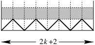
That this path contains $n_{i}=k$ particles, is also encoded in (40).

When the classical Gaussians are employed, equation (45) thus fails to account for the case of a zero length path. Use of the modified Gaussian remedies this, by permitting the case $n_{i}=-1$ . This may be viewed as an annihilation of the $k=0$ case of Fig. 9, which although appearing to be a particle (c.f. Lemma 3.12), arises through solely the action of the $B_{1}$ -transform followed by path extension.

Acknowledgments: We would like to thank Professor Y. Pugai for collaboration on an earlier stage of this work, and on related works, and for many useful discussions. His contributions to this work are gratefully acknowledged. We also wish to thank Professors A. Berkovich, B. McCoy and A. Schilling for many informative discussions on [7]. Finally, we wish to thank Professors M. Kashiwara and T. Miwa for the invitation to attend ‘Physical Combinatorics’ where a preliminary version of this work was presented, and for their excellent hospitality.

References

[1] A.K. Agarwal and D.M. Bressoud, Lattice paths and multiple basic hypergeometric series, Pac. J. Math. 136 (1989) 209–228.
[2] G.E. Andrews, The Theory of Partitions, Encyclopedia of Mathematics and its Applications, 2, Addison-Wesley, 1976.
[3] G.E. Andrews, R.J. Baxter, D.M. Bressoud, W.H. Burge, P.J. Forrester and G.X. Viennot, Partitions with prescribed hook differences, Europ. J. Comb. 8 (1987) 431–350.
[4] A.A. Belavin, A.M. Polyakov and A.B. Zamolodchikov, Infinite conformal symmetry in two-dimensional quantum field theory, Nucl. Phys. B241 (1984) 333–380.
[5] A. Berkovich and B.M. McCoy, Continued fractions and fermionic representations for characters of $M(p,p^{\prime})$ minimal models, Lett. Math. Phys. 37 (1996) 49–66.
[6] A. Berkovich and B.M. McCoy, The perturbation $\phi_{2,1}$ of the ${\mathcal{M}}(p,p+1)$ models of conformal field theory and related polynomial character identities, preprint math/9809066.
[7] A. Berkovich, B.M. McCoy and A. Schilling, Rogers–Schur–Ramanujan type identities for the $M(p,p^{\prime})$ minimal models of conformal field theory, Commun. Math. Phys. 191 (1998) 325–395.
[8] D.M. Bressoud, Lattice paths and the Rogers-Ramanujan identities, in Proceedings of the international Ramanujan centenary conference, Madras, 1987, ed. K. Alladi. Lecture Notes in Mathematics 1395, Springer, 1989.
[9] B. L. Feigen and D. B. Fuchs, Skew-symmetric differential operators on the line and Verma modules over the Virasoro algebra, Funct. Anal. and Appl. 17 (1982) 114–126.
[10] O. Foda, K.S.M. Lee, Y. Pugai and T.A. Welsh, Path generating transforms, preprint q-alg/9810043. To appear in Contemp. Math.
[11] O. Foda, K.S.M. Lee and T.A. Welsh, A Burge tree of Virasoro-type polynomial identities, Int. J. Mod. Phys, A 13 (1998) 4967–5012.
[12] O. Foda and T.A. Welsh, Melzer’s identities revisited, preprint q-alg/9811156. To appear in Contemp. Math.
[13] O. Foda and T.A. Welsh, Polynomial fermionic characters of Forrester-Baxter models, in preparation.
[14] P.J. Forrester and R.J. Baxter, Further exact solutions of the eight-vertex SOS model and generalizations of the Rogers-Ramanujan identities, J. Stat. Phys. 38 (1985) 435–472.
[15] G. Gasper and M. Rahman, Basic Hypergeometric Series, Encyclopedia of Mathematics and its Applications, 35, Cambridge University Press, 1990.
[16] M. Jimbo and T. Miwa, Algebraic Analysis of Solvable Lattice Models, CBMS 85, AMS, 1995.
[17] A. Rocha-Caridi, Vacuum vector representations of the Virasoro algebra, in Vertex Operators in Mathematics and Physics, eds. J. Lepowsky, S. Mandelstam and I.M. Singer, Springer, 1985.

On the combinatorics of Forrester-Baxter modelsThanks: Research supported by the Australian Research Council (ARC)

Abstract

0 Introduction

0.1 Motivation

0.2 Overview of content of paper

1 Paths

1.1 Paths and the (p,p′)(p,p^{\prime})-model

1.2 Weighting the paths

1.3 Bosonic generating function

2 Winged generating functions

2.1 Striking sequence of a path

Lemma 2.1

2.2 Path parameters

Lemma 2.2

2.3 Scoring generating functions

Lemma 2.3

Note 2.4

2.4 A seed

Lemma 2.5

2.5 Partitions

Lemma 2.6

3 The ℬ{\mathcal{B}}-transform

3.1 Path-dilation

Lemma 3.1

Note 3.2

Lemma 3.3

Corollary 3.4

Lemma 3.5

Lemma 3.6

3.2 Particle insertion

Lemma 3.7

3.3 Particle moves

Lemma 3.8

3.4 The ℬ3{\mathcal{B}}_{3}-transform

Lemma 3.9

Lemma 3.10

Note 3.11

3.5 Particle content of a path

Lemma 3.12

Lemma 3.13

Corollary 3.14

4 The 𝒟{\mathcal{D}}-transform

Lemma 4.1

Lemma 4.2

Corollary 4.3

4.1 The ℬ​𝒟{\mathcal{B}}{\mathcal{D}}-pair

Lemma 4.4

Lemma 4.5

Corollary 4.6

Lemma 4.7

5 The structure of the (p,p′)(p,p^{\prime})-model

5.1 Continued fractions

5.2 The Takahashi and string lengths

6 Segmenting the model

6.1 Model comparisons

Lemma 6.1

Lemma 6.2

Lemma 6.3

Lemma 6.4

6.2 Interfacial retention

Lemma 6.5

Lemma 6.6

Corollary 6.7

Corollary 6.8

7 Extending and truncating paths

7.1 Extending paths

Lemma 7.1

Lemma 7.2

Lemma 7.3

Lemma 7.4

7.2 Truncating paths

Lemma 7.5

Lemma 7.6

8 Fermionic expressions

8.1 Results

Theorem 8.1

Theorem 8.2

8.2 Carrying out the induction

Lemma 8.3

Lemma 8.4

1.1 Paths and the $(p,p^{\prime})$ -model

3 The ${\mathcal{B}}$ -transform

3.4 The ${\mathcal{B}}_{3}$ -transform

4 The ${\mathcal{D}}$ -transform

4.1 The ${\mathcal{B}}{\mathcal{D}}$ -pair

5 The structure of the $(p,p^{\prime})$ -model

8.3 The $m$ $n$ -system