Equivariant self-similar wave maps from Minkowski spacetime into -sphere
Abstract
We prove existence of a countable family of spherically symmetric self-similar wave maps from Minkowski spacetime into the 3-sphere. These maps can be viewed as excitations of the ground state wave map found previously by Shatah. The first excitation is particularly interesting in the context of the Cauchy problem since it plays the role of a critical solution sitting at the threshold of singularity formation. We analyze the linear stability of our wave maps and show that the number of unstable modes about a given map is equal to its excitation index. Finally, we formulate a condition under which these results can be generalized to higher dimensions.
1 Introduction.
Wave maps, defined as harmonic maps from a spacetime into a Riemannian manifold , have been intensively studied during the past decade (see the recent review [1]). The interest in wave maps (sometimes called also sigma models) stems from the fact that they contain many features of more complex relativistic field models but are simple enough to be tractable rigorously. In particular, the investigation of questions of global existence and formation of singularities for wave maps can give insight into the analogous, but much more difficult, problems in general relativity. With this motivation we have recently studied numerically the development of singularities for wave maps from Minkowski spacetime into the -sphere [2]. In this case it was known that: (i) solutions with small initial data exist globally in time [3, 4]; (ii) there exist smooth initial data which lead to blow-up in finite time. An example of (ii) is due to Shatah [5] who constructed a spherically symmetric self-similar wave map of the form . This solution is perfectly smooth for but it breaks down at . Our numerical simulations [2] strongly suggest that the self-similar blow-up found by Shatah is generic in the sense that there is a large set of initial data which comprise the basin of attraction of the solution . In particular, it seems that all initial data of nonzero degree (which by definition are not small in the sense of [3, 4]) blow up in this universal self-similar manner. The dynamical evolution of degree zero wave maps is more interesting because, depending on the “size” of initial data, the solutions either exist globally in time converging to the vacuum (this scenario is usually referred to as dispersion), or blow-up in finite time (where, as before, the blow-up profile is given by ). Thus, in this case there arises a natural question of determining the boundary between the basins of attraction of these two generic asymptotic behaviors. In [2] we studied this question numerically by evolving various one-parameter families of degree zero initial data interpolating between blow-up and dispersion. A typical initial data in this class is a gaussian with varying amplitude. We found that the initial data lying on the boundary between the basins of attraction of the solution and the vacuum solution converge asymptotically to a certain codimension-one attractor which is self-similar. This suggested that, besides , the model admits another self-similar solution, call it , which has exactly one unstable direction. This expectation was confirmed numerically in [2]. In a sense, the solution can be thought of as the excitation of the ground state solution .
The aim of this paper is to give a rigorous proof of existence of a countable family of spherically symmetric self-similar wave maps from Minkowski spacetime into the -sphere. The above mentioned solutions and are the first two elements of this family. The proof is based on a shooting technique very similar to the one used by us in the case of harmonic maps between 3-spheres [6].
2 Preliminaries.
A wave map is a map from a spacetime with metric into a Riemannian manifold with metric which is a critical point of the action
| (1) |
The associated Euler-Lagrange equations
| (2) |
constitute the system of semilinear wave equations, where ’s are the Christoffel symbols of the metric . In this paper we consider the case where , dimensional Minkowski spacetime, and , the unit -sphere. In polar coordinates on and the respective metrics are
| (3) |
and
| (4) |
where and are the standard metrics on , and . We consider spherically symmetric maps of the form
| (5) |
Then the action (1) reduces to
| (6) |
and the corresponding Euler-Lagrange equation is
| (7) |
This equation is invariant under dilations: if is a solution of equation (7), so is . It is thus natural to look for self-similar solutions of the form
| (8) |
where is a positive constant. As mentioned in the introduction such solutions are important in the context of the Cauchy problem for equation (7) since they appear in the dynamical evolution as intermediate or final attractors. Substituting the ansatz (8) into (7) we obtain the ordinary differential equation
| (9) |
where and . For we have .
It is sufficient to consider equation (9) only inside the past light cone of the point , i. e., for . This constitutes the two-point singular boundary value problem with the boundary conditions
| (10) |
which are dictated by the requirement of smoothness at the endpoints. Once a solution of equation (9) satisfying the conditions (10) is constructed, it can be easily extended to [5]. Note that solutions of (9) and (10) are the critical points of the functional
| (11) |
which, as was pointed out by Shatah and Tahvildar-Zadeh [7], can be interpreted as the energy for harmonic maps from the hyperbolic space into the upper hemisphere of . Shatah [5] showed that is bounded from below over the -space of functions satisfying (10) and attains an infimum at a smooth function , the ground state solution of equation (9). Independently, Turok and Spergel [8] found this solution in closed form
| (12) |
The central result of this paper is
Theorem 1
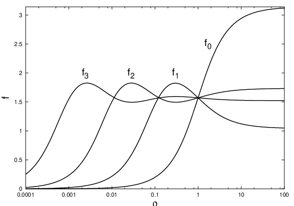
There exist a countable family of smooth solutions of equation (9) satisfying the boundary conditions (10). The index denotes the number of intersections of with the line (the equator of ) on .
Before proving this theorem in the next section, we present now some numerical results. As will be shown below the solutions satisfying form a one-parameter family with asymptotics near , while the solutions satisfying form a one-parameter family with asymptotics near . The solutions are obtained by a standard shooting-to-a-fitting-point method, that is by integrating equation (9) away from the singular points and in the opposite directions with some trial parameters and and then adjusting these parameters so that the solution joins smoothly at the fitting point. The discrete set of pairs generated in this way and the energies characterizing the solutions are shown below for .
|
3 Proof of Theorem 1
To prepare the ground for the proof of Theorem 1 we first discuss some basic properties of solutions of equation (9). It is convenient to use new variables defined by
| (13) |
The range of is from (for ) to (for ). Note that the number of intersections of with the line is the same as the number of zeros of . In these new variables equation (9) becomes
| (14) |
and the boundary conditions (10) translate into
| (15) |
where the sign in the last expression, obviously allowed by the reflection symmetry , is introduced for convenience.
Lemma 1
For any there exists a unique global solution to equation (14) such that
| (16) |
as .
Proof: Defining , let us rewrite equation (14) as the system of two integral equations
| (17) |
Following the standard procedure we solve (17) by iteration, setting
| (18) |
with the starting values and . It can easily be shown that the mapping defined by (18) is contractive for any finite , hence the sequence converges to a solution of equation (14). The proof of uniqueness is also routine so we omit it.
Definition 1
A solution of equation (14) starting at with the asymptotic behavior (16) will be called the -orbit. Without loss of generality we assume that . The -orbit which satisfies will be called a connecting orbit.
Remark 1: In the following whenever we say “a solution” we
always mean the
-orbit. Also, when we say that some property holds for all we
always mean for all . We use
to denote .
Remark 2: The endpoints of connecting orbits
are saddle-type critical points of the asymptotic () autonomous equation
. One can easily show (cf. [6]) that
the connecting orbits converge to these points along the
one-dimensional stable manifolds .
The following function, defined for -orbits, will play a crucial role in our analysis
| (19) |
We have
| (20) |
so is increasing (unless is a constant solution). Equations (19) and (20) imply that if for some ( and is not identically equal to ) then for , hence . Thus, if a -orbit crosses the line , then and tend monotonically to .
Lemma 2
A -orbit (with nonzero ) which satisfies for all , is a connecting orbit.
Proof: We showed above that if for some , then tends to infinity, hence implies that for all , so exists. Thus, which means by (20) that and next by (19) that exists, implying that also exists. By equation (14), since otherwise contradicting . Hence, or . To conclude the proof note that the latter implies which in view of (20) is possible only if , that is .
The next two lemmas describe the behavior of -orbits for small and large values of the shooting parameter , respectively.
Lemma 3
If is sufficiently small then the solution has arbitrarily many zeros.
Proof: Define . The function satisfies
| (21) |
with the asymptotic behavior as . As , the solutions of equation (21) tend uniformly on compact intervals to the solution of the limiting equation
| (22) |
with the asymptotic behavior as . The solution can be found in closed form in terms of the hypergeometric function but for the purpose of the argument it is enough to observe that is oscillating at infinity, since this implies that the number of zeros of increases to infinity as tends to zero.
Lemma 4
If is sufficiently large then the solution increases monotonically to .
Proof: As in the proof of Lemma 3, we use a scaling argument. This time, we define . The function satisfies
| (23) |
with the asymptotic behavior as . As , the solutions of equation (23) tend uniformly on compact intervals to the solution of the limiting equation
| (24) |
that is to . Thus, on any compact interval the solution stays arbitrarily close to if is sufficiently large. In particular, strictly increases up to some where . Since , by the argument following (20) tends monotonically to .
Now we are ready to prove Theorem 1. The proof will the immediate corollary of the following proposition
Proposition 1
There exists a decreasing sequence of positive numbers , , such that the corresponding -orbits are connecting orbits with exactly zeros for . Morever, .
Proof: The proof is based on an inductive application of the standard shooting argument. Let strictly increases up to some where . Let . By Lemma 4 the set is nonempty and by Lemma 3 . The -orbit cannot cross the line at a finite because the same would be true for nearby -orbits with , violating the definition of . Thus, the -orbit stays in the region for all , and therefore due to Lemma 2 it is a connecting orbit. By definition the -orbit has no zeros for .
To make the inductive step we need one more lemma.
Lemma 5
If for sufficiently small , then the solution increases up to some where it attains a positive local maximum and then decreases monotonically to .
Proof: By the definition of there must exist a point where . Since by (14) a solution cannot have a local minimum if , it follows that there must be a point where (otherwise the -orbit would contradict Lemma 2). The idea of the proof is to show that provided that is sufficiently small. As argued above this implies that for decreases monotonically to . In the following we drop the index on . From (19) we have
| (25) |
In order to estimate the last integral note that for
| (26) |
so . Inserting this into (24) gives
| (27) |
The right-hand side of this inequality is an increasing function of which exceeds if , as can be checked by direct calculation. The value will fall into that interval if is sufficiently small because by continuous dependence of solutions on initial conditions, as . This concludes the proof of Lemma 5.
Having Lemma 5 we return now to the proof of Proposition 1. Let increases up to some where it attains a positive local maximum and then decreases monotonically up to some where }. Let . Due to Lemma 5 the set is nonempty and by Lemma 3 is strictly positive. Using the same argument as above we conclude that the -orbit must stay in the region for all , so it is a connecting orbit (asymptoting to ). By definition the -orbit has exactly one zero for .
The subsequent connecting orbits are obtained by the repetition of the above construction. Since the sequence is decreasing and bounded below by zero, it has a nonnegative limit. Suppose that . The -orbit cannot leave the region for a finite because the set of such orbits is clearly open. Thus, the -orbit is a connecting orbit with some finite number of zeros. But this contradicts the fact that the number of zeros of -orbits increases with . We conclude therefore that . This completes the proof of Proposition 1. Returning to the original variables and , and using the notation , we have with and , as claimed in Theorem 1.
We end this section with a remark about the large limit. From , it follows that for any finite . The limiting solution (or ) is a singular map which geometrically corresponds to the map into the equator of . The “energy” of this map provides the upper bound for the “energies” of critical points of (11) (we write “energy” is quotation marks to emphasize that the functional (11) is not the true conserved energy associated with the action (6)). As follows from the proof of Lemma 3, the behavior of connecting orbits with large (and consequently small ) can be approximated by the solution of equation (22), namely on where tends to infinity as . This fact can be used to prove some remarkable scaling properties of connecting orbits in the limit of large .
For example one can show that (see the table in Section 2)
| (28) |
For more detailed discussion of this issue we refer the reader to [6] where the analogous behavior in the case of harmonic maps between spheres was derived.
4 Stability
The role of self-similar solutions in the evolution depends crucially on their stability with respect to small perturbations. This problem was analysed by us in [2] by mixed analytic-numerical methods. In particular, we provided evidence towards the conjecture that the solution is asymptotically stable and, as such, has an open basin of attraction. To make the results obtained in [2] rigorous is a formidable task. In this section we discuss the first (easy) step in achieving this goal, namely we determine the character of the spectrum of the linearized operator around the solutions . A somewhat different but equivalent version of the linear stability analysis was presented in [2].
We restrict attention to the interior of the past light cone of the point and define the new time coordinate . In terms of and , Eq.(7) becomes
| (29) |
Of course, this equation reduces to Eq.(7) if the solution is self-similar, that is -independent. Following the standard procedure we seek solutions of (29) in the form . Neglecting the terms we obtain a linear evolution equation for the perturbation
| (30) |
Substituting into (30) we get the eigenvalue problem
| (31) |
Note that the principal part of the operator is the radial Laplacian on the hyperbolic space . We consider this problem in the space of functions which are square-integrable on the interval with respect to the natural inner product on , that is
| (32) |
In this function space is self-adjoint hence its spectrum is real. Both endpoints are of the limit-point type. Near the leading behavior of solutions of (31) is where , so admissible solutions behave as
| (33) |
Near the leading behavior is where so eigenfunctions must have and behave as (up to a normalization constant)
| (34) |
All belong to the continuous spectrum of . The case will be treated separately below. Note that this eigenvalue problem has the symmetry (that is why we wrote rather than in the ansatz for ). Each eigenvalue gives rise to an unstable mode which grows exponentially as . To find the eigenvalues we need to solve (31) on the interval with the boundary conditions (33) and (34). In [2] we did this numerically (for ) by shooting the solutions from both ends and matching the logarithmic derivatives at a midpoint. For example, for we got ; for we got . Our numerics strongly suggested that the point spectrum of the operator around the solution has exactly positive eigenvalues (). Now, we will give a simple proof of this property.
The proof is based on the observation that the solution with corresponds to the gauge mode which is due to the freedom of choosing the blowup time . To see this, consider a solution . In terms of the similarity variables and , we have
| (35) |
In other words, each self-similar solution generates the orbit of solutions of (29) parametrized by . It is easy to verify that the generator of this orbit
| (36) |
solves (30), thus satisfies (31) with 11 1 We emphasize that is not an eigenvalue because is not square-integrable at . Hovewer, this solution is distinguished from the rest of the continuous spectrum by the fact that it is subdominant at (such a solution is sometimes referred to as a pseudo-eigenfunction).. Since has exactly zeros on (because has extrema), it follows by the standard result from Sturm-Liouville theory that there are exactly positive eigenvalues, as conjectured in [2]. To summarize, we showed that the self-similar solution has exactly unstable modes, which means in particular that the solution is linearly stable.
Remark. If we view the solutions as harmonic maps from the hyperboloid into , then the eigenvalue problem (31) determines the spectrum of the Hessian of the energy functional (11)
| (37) |
Within this approach the argument given above can be rephrased in terms of the Morse index. In particular, it implies that the Morse index of the solution is zero, in agreement with Shatah’s result that is a local minimum of the energy functional (11). Note that in this context the gauge mode acquires a geometrical interpretation as the perturbation induced by , the conformal Killing vector field on ,
| (38) |
Aside, we remark that by solving (31) one can show that the Morse index of the singular map is infinite. This fact could be probably used to give an alternative proof of Theorem 1 via Morse theory methods using the ideas of Corlette and Wald developed recently in the case of harmonic maps between spheres [10].
5 Generalization to higher dimensions
The proof of Theorem 1 is rather robust which suggests that the result can be generalized in various directions. One possibility, which will not be pursued here, is to consider more general nonconvex targets22 2 For example, one can easily verify that the proof of Theorem 1 goes through if the metric (4) is replaced by where the function satisfies the following conditions (cf. [11]): (i) and ; (ii) is monotone increasing from up to some where it attains a maximum.. Another possibility is to consider the analogous problem in higher dimensions, that is wave maps , where , dimensional Minkowski spacetime, and , the unit -sphere. At the same time one can relax the equivariance ansatz (5) by admitting the maps of the form
| (39) |
where is a homogeneous harmonic polynomial of degree . The ansatz (5) is the special case of (39) with . Assuming self-similarity we obtain the analogue of Eq.(9)
| (40) |
where . As before, we want to construct smooth solutions on the interval satisfying the boundary conditions (10). Standard analysis of the behavior of such solutions at the endpoints yields that near and . Note that the latter implies that the desired smooth solutions can exist only if the dimension is odd. Although Eq.(40) looks more complex than (9), the same change of variables as in (13) transforms (40) into
| (41) |
which has the same form as (14) apart from the change of constant coefficients. Now, let us see which steps of the shooting argument from Section 3 are effected by this change of coefficients. Lemma 1 holds with the asymptotic behavior near replaced by . Lemmas 2 and 4 remain valid because their proofs are dimension independent. The only fact which is dimension sensitive is Lemma 3, because in dimensions the limiting equation analogous to (22) reads
| (42) |
so Lemma 3 is true iff the solution is oscillating at infinity, that is, . This imposes the condition
| (43) |
Under this condition the proofs of Lemma 5 and Proposition 1 remain basically unchanged, thus we have
Theorem 2
For each odd and satisfying the condition (43), there exist a countable family of smooth solutions of equation (40) satisfying the boundary conditions (10). The index denotes the number of intersections of with the line on .
This theorem extends the recent result of Cazenave, Shatah, and Tahvildar-Zadeh [11] who proved existence of the ground state solution in odd dimensions under the condition (43) using variational methods.
Acknowledgments
I thank Robert Wald for discussions and Arthur Wasserman for reading the manuscript and helpful remarks. This research was supported in part by the KBN grant 2 P03B 010 16.
References
- [1] M. Struve, Wave maps, Progress in Nonlinear Differential Equations and their Applications, vol.29 (Birkhauser, 1997).
- [2] P. Bizoń, T. Chmaj, and Z. Tabor, Dispersion and collapse of wave maps, math-ph/9912009, to appear in Nonlinearity.
- [3] T. Sideris, Global existence of harmonic maps in Minkowski space, Comm. Pure Appl. Math. 42, 1-13 (1989).
- [4] M. Kovalyov, Long-time behaviour of solutions of a system of nonlinear equations, Comm. PDE 12, 471-501 (1987).
- [5] J. Shatah, Weak solutions and development of singularities of the SU(2) -model, Comm. Pure Appl. Math. 41, 459-469 (1988).
- [6] P. Bizoń, Harmonic maps between 3-spheres, Proc. Roy. Soc. London A451, 779-793 (1995).
- [7] J. Shatah and A. Tahvildar-Zadeh, On the Cauchy problem for equivariant wave maps, Comm. Pure Appl. Math. 47, 719-754 (1994).
- [8] N. Turok and D. Spergel, Global texture and the microwave background, Phys. Rev. Lett. 64, 2736-2739 (1990).
- [9] S. Äminneborg and L. Bergström, On selfsimilar global textures in an expanding universe, Phys. Lett. B362, 39–43 (1995).
- [10] K. Corlette and R. M. Wald, Morse theory and infinite families of harmonic maps between spheres, math-ph/9912001.
- [11] T. Cazenave, J. Shatah, and A. Tahvildar-Zadeh, Harmonic maps of the hyperbolic space and development of singularities for wave maps and Yang-Mills fields, Ann. Inst. H. Poincare Phys. Theor. 68, 315–349 (1998).