CONTACT TOPOLOGY AND HYDRODYNAMICS III: KNOTTED FLOWLINES
| JOHN ETNYRE | ROBERT GHRIST |
| Department of Mathematics | School of Mathematics |
| Stanford University | Georgia Institute of Technology |
| Stanford, CA 94305 | Atlanta, GA 30332-0160 |
Abstract
We employ the relationship between contact structures and Beltrami fields derived in part I of this series to construct steady nonsingular solutions to the Euler equations on a Riemannian whose flowlines trace out closed curves of all possible knot and link types simultaneously. Using careful contact-topological controls, we can make such vector fields real-analytic and transverse to the tight contact structure on .
AMS classification: 57M25, 76C05, 58F25, 58F05.
1 Introduction
This work considers the paths of particles in a three-dimensional steady inviscid fluid flow. The relationship between Lagrangian dynamics and knot theory comes from the observation that any particle path which is periodic traces out a simple closed curve — a knot. We note the historical significance of this relationship: Lord Kelvin’s notion that matter was built from knotted vortex tubes in the æther initiated his and Tait’s investigations into knot types, in the hope that the structure of the periodic table would be recovered [Tho69]. Thus the mathematical classification of knot types began, arguably, as a problem in fluid dynamics.
We consider solutions to the Euler equations for a perfect incompressible fluid, restricting attention to steady flows of high regularity for simplicity. In a previous paper, we showed that unknotted orbits are forced in steady real-analytic Euler flows on .
Theorem ([EG99])Any steady Euler flow on a Riemannian must possess a closed flowline which bounds an embedded disc: an unknot.
In this work, we consider the opposite end of the spectrum, asking “What is possible” rather than “What is forced?” The result of our inquiry is that the most complicated and intricate knotting and linking phenomena known are present within the simplest class of fluid flows.
Main Theorem There exists a steady nonsingular solution to the Euler equations on a Riemannian which possesses periodic flowlines of all possible knot and link types simultaneously.
This theorem answers a question in [Wil98]. General vector fields on having all knots and links as closed orbits were discovered by Ghrist [Ghr97, GHS97], using the template construction of Birman and Williams [BW83a, BW83b]. It is by no means clear that such phenomena can arise within fluid flows — indeed, a large class of solutions (the integrable fields) of necessity possess a very restricted class of knot types. We are thus forced to consider the contact geometry and topology associated to Euler flows, as elucidated in part I of this series [EG98]. We translate the problem of constructing topologically complicated Euler flows to the problem of finding a certain kind of contact form on . A careful construction yields a solution which is furthermore transverse to the standard tight contact structure on (see §2.2 for definitions).
The advantage of working in the realm of contact topology is that it is genuinely topological: one may perform surgery or cut-and-paste constructions on contact forms, and still have a solution to the Euler equations at the end of the day. However, the price paid is a geometric one — the standard Riemannian structure is necessarily altered by our constructions. Thus the Euler flows we construct satisfy the Euler equations for some Riemannian structure almost certainly different than the standard one. It remains an open (and interesting) problem to find such a knotted steady flow on Euclidean (or to find an obstruction).
In many respects, this paper is inspired by the pioneering work of Moffatt, who, in a series of papers [Mof85, Mof86] discusses Euler flows “with arbitrarily complex topology.” What is meant by this is the construction of steady solutions to the Euler equations on Euclidean which realize the same orbit topology as any given volume-preserving flow on the space. These results have the advantage of staying within the class of Euclidean metrics. However, there are two caveats associated to this work: (1) the techniques do not guarantee a continuous solution — so-called “vortex sheet” discontinuities may develop; (2) the proof itself relies crucially upon the global-time existence of solutions to the Navier-Stokes equations (with an alternate viscosity term). Such an existence theorem is to date unknown.
2 Background
Since the results of this paper require techniques and perspectives from a variety of otherwise disjoint subjects, we include a substantial amount of background material. The expert reader may skip the following subsections as appropriate.
2.1 Beltrami fields
For information on a topological approach to the relevant equations of fluid dynamics, see the recent monograph [AK98].
The fundamental equations describing the velocity field of a perfect incompressible fluid flow on a Riemannian three-manifold with metric and distinguished volume form are the Euler equations. We present the equations as an exterior differential system, using to denote the Lie derivative along and to denote contraction by :
| (1) |
Here is a reduced pressure function, and the vorticity, , is defined by the relation . A vector field is said to be Eulerian if it satisfies Equation (1) for some pressure function .
It follows from Bernoulli’s Theorem that, for a steady Eulerian flow, the function is an integral of motion for flowlines. Hence, as long as does not vanish on open sets, steady Eulerian fields must be integrable. From the Fomenko-style approach to integrable systems, it follows that the periodic orbits of such a flow must have especially simple knot types (see Theorem 3.1). The only alternative, then, is that , which translates to the condition that . In other words, is everywhere collinear with its curl. This class of vector fields is of particular importance.
Definition 2.1
A volume-preserving vector field on a Riemannian manifold is a Beltrami field if for some function on . A rotational Beltrami field is one for which ; that is, the curl is nonsingular.
Beltrami fields possess several interesting geometric, analytic, and dynamical features: see [AK98, EG98] for more information. A key example of a Beltrami field is the class of ABC fields:
| (2) |
Here, are constants, and the vector field is defined on the three-torus . By symmetry in the variables and parameters, we may assume without loss of generality that . Under this convention, the vector field is nonsingular if and only if (see [DFG+86]). This particular vector field exhibits the so-called “Lagrangian turbulence” — there are apparently large regions of nonintegrability and mixing within the flow.
Beltrami fields occupy an important place not only within hydrodynamics, but also within the study of magnetic fields and plasmas (where they are known as force-free fields). As such, our results imply the existence of complex knotting within these settings as well.
2.2 Contact topology
We provide a brief description of the relevant concepts in dimension three, though the basic definitions and relationships extend to all odd dimensions. More comprehensive treatments of this subject are available in [MS95, Aeb94].
A contact form on a three-manifold is a 1-form such is nowhere-vanishing. A contact structure on is the kernel of a (locally defined) contact form; i.e., . From the Frobenius integrability theorem, it follows that a contact structure is a totally nonintegrable plane field distribution on .
The interesting (and difficult) problems in contact geometry are all of a global nature: Darboux’s Theorem (see, e.g., [MS95, Aeb94]) implies that all contact structures are locally contactomorphic, or diffeomorphic preserving the plane fields. Standard normal forms for a point include [Cartesian coordinates] and [polar coordinates]. A similar result holds for a surface in a contact manifold as follows. Generically, will be a line in This line field integrates to a singular foliation called the characteristic foliation of . The Moser-Weinstein Theorem implies, as in the single-point case of Darboux’s Theorem, that determines the germ of along .
Contact structures are thus implicitly global objects. Their global properties in dimension three depend crucially upon a dichotomy first explored by Bennequin [Ben83] and Eliashberg [Eli89]. A contact structure is overtwisted if there exists an embedded disc in whose characteristic foliation contains a limit cycle. If is not overtwisted then it is called tight. Eliashberg [Eli89] has completely classified overtwisted contact structures on closed 3-manifolds — the geometry of overtwisted contact structures reduces to the algebra of homotopy classes of plane fields. Such insight into tight contact structures is slow in coming.
The standard contact structure on the unit is given by the kernel of the 1-form
| (3) |
The contact structure is the plane field orthogonal to the fibres of the Hopf fibration (orthogonal with respect to the metric on the unit 3-sphere induced by the standard metric on ). It is a foundational result that this contact structure is tight [Ben83]; moreover, it is the unique tight structure on up to orientation and contactomorphism [Eli92].
One recently successful method for analyzing contact structures is to consider the dynamical structures imposed by a defining 1-form. Given a contact form , the Reeb field associated to is the unique vector field such that
| (4) |
There are intricate relationships between the dynamics of Reeb fields and the tight/overtwisted data of the underlying contact structure [Hof93, HWZ96].
The relationship between contact structures and solutions to the Euler equations is explored in [EG98], where the following correspondence theorem is proved:
Theorem 2.2 (Etnyre & Ghrist [EG98])
On a fixed 3-manifold , the class of vector fields which are nonsingular rotational Beltrami fields for some Riemannian metric and preserved volume form is equivalent to the class of vector fields which are nonsingular rescalings of the Reeb field for some contact form.
In other words, given any (nonsingular, rotational) Beltrami field there exists a natural transverse contact form whose Reeb field is a reparametrization of the Beltrami field, and given any reparametrized Reeb field, there exists a natural Riemannian structure and volume making it Beltrami. For an un-rescaled Reeb field (normalized to unit length with respect to the contact form), the conserved volume may be chosen to be that induced by the Riemannian metric.
Note that the class of Beltrami fields is geometric in nature, and is not at all well-behaved with respect to perturbations, etc. On the other hand, the Reeb fields and their rescalings are quite flexible: a fact we shall take advantage of in §3. Shedding the metric constraints thus transforms geometric problems to topological ones.
2.3 Template theory
For a complete treatment of this subject, see [GHS97].
The problem of knotted orbits in vector fields on three-manifolds is full of surprises, beginning with the pioneering work of Williams in the late 1970’s to understand solutions to the Lorenz equations [Wil77]. In developing the geometric model for the Lorenz equations [GW79], Williams considered branched surfaces. In a pair of papers with Birman [BW83a, BW83b], the knot-theoretical implications of these ideas were brought forth in the notion of a knotholder, later rechristened a template [HW85].
Definition 2.3
A template is a compact branched 2-manifold with boundary supporting a smooth expansive semiflow.

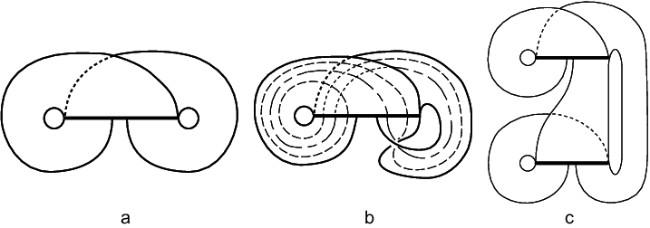
Templates have a description in terms of charts: every template is diffeomorphic to the branched surface obtained by gluing together a finite number of joining and splitting charts (illustrated in Figure 1) end-to-end respecting the semiflows. Examples of embedded templates appear in Figure 2.
The semiflow on a template is “overflowing” in the sense that it is not defined on the gaps between strips of the splitting charts. This is inconsequential as one is only interested in the invariant sets of the semiflow; hence, the gaps are often back-propagated to the branchlines in figures. Due to the expanding nature of the dynamics on a template, the invariant set consists of the suspension of a subshift of finite type, generated by the symbolic dynamics of the Markov partition induced by the branch lines. Specifically, the branchlines are partitioned by the exit sets into a finite number of intervals , each of which gets stretched under the semiflow to cover two other partition elements. The expansive nature of the semiflow implies that forward orbits on the template are in bijective correspondence with the semi-infinite admissible symbol sequences in the alphabet induced by — see [GHS97] for more information and examples.
Templates arise naturally in the context of nontrivial hyperbolic invariant sets in a flow on a three-manifold . Let denote such an invariant set. The Template Theorem of Birman and Williams implies that there exists an embedded template such that the periodic orbits of are in bijective correspondence with those of the semiflow on , and that, furthermore, this correspondence preserves all knotting and linking information. Hence, to obtain information about knotted periodic orbits in , one simply analyzes the template . The essence of their proof is to collapse a foliation by strong stable manifolds — identifying all orbits with the same asymptotic future. Clearly, this preserves the periodic orbit set and its embedding properties.
Given the Template Theorem above, one may proceed to analyze the knotting and linking properties of various systems. This analysis has been conducted for the (geometric) Lorenz attractor [BW83a], the suspension of the Smale horseshoe [BW83b, HW85, Hol86, GH93], systems associated with a Josephson junction [Hol87], flows near Shilnikov homoclinic orbits [GH96], and flows transverse to fibred links in with pseudo-Anosov monodromy [BW83b, Ghr97].
The question of whether a flow on can support all knots at once may thus be addressed from the point of view of templates. In [Ghr97] it was shown that there exist universal templates in which contain closed orbits of all possible knot (and link) types. The canonical example appears in Figure 2(c). The way in which the knots lie within the template is highly nontrivial: the simplest known example of a figure-eight knot on this template crosses the branchlines millions of times [Ghr97, GHS97].
Given a flow on which supports a hyperbolic invariant set modeled by a template, it is in general impossible to determine if this template is universal: no general computable criterion is known. However, the only obstruction to being universal is on the embedding level — any (abstract) template can be embedded in so as to be universal [GHS97, Thm. 3.3.5]. A particularly useful result concerns the Lorenz-like templates, , pictured in Figure 3. Also useful in the sequel are the Lorenz-like templates with the branchline crossing reversed: denote these by , with the sign convention as in Figure 3.

Theorem 2.4 (Ghrist [Ghr97])
In the case where the product , the Lorenz-like template is universal if and only if and .
3 A Reeb field with all knots
In this section, we prove the existence of a Reeb field on the tight 3-sphere whose flow has a hyperbolic invariant subset which collapses to a universal template. We begin by noting the necessity of the contact-topological techniques outlined in §2.1. Recall that the class of zero-entropy knots consists of those knots obtainable from the unknot by iterating the operations of cabling and connected sum [EG99]. Such knots are a very small subclass of knots, excluding such large classes as hyperbolic knots (knots whose complement in supports a hyperbolic geometry).
Theorem 3.1 (Etnyre & Ghrist [EG99])
Let denote a steady nonsingular solution to the Euler equations on a Riemannian 3-manifold. If is not a Beltrami field, then every periodic orbit of must be a zero-entropy knot.
Hence we conclude that it is necessary to consider Reeb (i.e., Beltrami) fields as the only possibility for constructing highly regular steady flows with all knots.
Lemma 3.2
There exists a Reeb field on some tight contact 3-manifold possessing a nontrivial one-dimensional hyperbolic invariant set.
Proof: We give an explicit example on the 3-torus. Consider the ABC equations of §2.1. From Equations (2) and (4) it follows that the ABC fields lie within the kernel of the derivative of the 1-form
| (5) |
and that this is a contact form when the vector field is nonsingular. Denote by the induced contact structure on . This contact structure is always tight [EG98].
In the limit where , and , the vector field takes on the particularly simple form
| (6) |
It is straightforward to demonstrate that there exists a pair of periodic orbits whose stable and unstable invariant manifolds intersect each other nontransversally (see, e.g., [DFG+86]). Upon perturbing to a small nonzero value, this connection may become transverse. Indeed, a Melnikov perturbation analysis reveals precisely this fact [HZD98, ZKLH93, Gau85]. It thus follows from the Birkhoff-Smale Homoclinic Theorem that there exists parameters for which Equation (2) possesses a nontrivial 1-d hyperbolic invariant set as a solution: a suspended 2-shift.
At this stage, there are two possible ways to proceed. One could perform a straightforward surgery construction on a tubular neighborhood of the hyperbolic 2-shift above to obtain a Reeb field on having an invariant set modeled by a Lorenz-like template. However, it is not at all obvious that the contact structure so induced on is the tight one, especially under the constraint that the framing on the surgery coefficients be such that the resulting template is universal. Thus, we turn to a method of constructing a contact embedding into the tight 3-sphere handle-by-handle.
In order to embed this hyperbolic 2-shift into the tight three-sphere, we require the following technical lemma for controlling characteristic foliations on annuli. This Lemma has appeared in the preprint [Col99, Lemma 3.3], as well as in [ML98, Lemma 4.4] in a slightly more restricted setting. We include the simple proof for completeness and clarity.
Lemma 3.3
Given any orientation-preserving diffeomorphism , there exists a smooth annulus in such that (1) is transverse to the contact structure ; (2) consists of the circles ; and (3) the monodromy obtained by sliding along leaves of from to is precisely the map .
Proof: Begin with the annulus and outfit it with any foliation such that (1) the slope of the leaves of is always negative; and (2) the monodromy along exists and is given by . Such a foliation clearly exists. To realize as the characteristic foliation of an annulus in , simply compute the slope of the leaves of in coordinates. Then, the annulus has characteristic foliation given by , since is defined by the relation . To fix the boundary of , simply choose so that the slope at is precisely : this in no ways hinders the choice of monodromy.
Theorem 3.4
There exists a hyperbolic invariant suspended 2-shift in the Reeb field of Lemma 3.2 and a tubular neighborhood of , , diffeomorphic to a genus-2 handlebody such that embeds contactomorphically into .
Proof: Choose a closed orbit in the hyperbolic invariant set from Lemma 3.2 and an unknotted curve transverse to in . By the Moser-Weinstein Theorem, there exists a neighborhood of and a contact embedding taking to .
Let denote a small disc transverse to the flow at a point . It is a standard result from the theory of hyperbolic dynamics that the periodic orbits are dense in the invariant 2-shift; thus, choose a closed orbit in the invariant set intersecting once in the point : such an orbit exists for sufficiently small.
There exists a “small” suspended 2-shift that is generated by and as follows. There exists a Markov partition by a pair of rectangles on , such that the fixed points of the return map on consists of the pair of points and . From basic symbolic dynamics it follows that the Poincaré return map restricted to possesses a hyperbolic invariant 2-shift. Let denote a flowbox neighborhood of , and let and denote, respectively, the solid cylinders in the complement of traced out by a small neighborhood of and (resp.) under the flow, as illustrated in Figure 4. The union is thus a genus-2 handlebody neighborhood of .

Note that the contactomorphism can be defined on and , since the size of the Markov rectangles is bounded by the size of chosen arbitrarily small. Once this is fixed, however, the size of the neighborhood of cannot then be chosen to be arbitrarily small, while still containing an invariant 2-shift. Nor can we fix and and then choose arbitrarily small neighborhoods; hence, one is impeded from employing a Moser-Weinstein type argument to extend to . We circumvent this by using the rigidity of the tight contact structures implicated in the construction. The remainder of this proof is rather technical — we organize the more intricate steps in a series of claims.
Denote by the smooth annulus with boundary components and on . Let and denote the -images of , and respectively. Denote by the image of . This curve connects the two disc-components of . Choose an arc in transverse to connecting the ends of such that is a smooth simple closed curve which bounds an embedded disc in the complement of . This curve will become the core of the image of in .
Claim 1: There exists a cylinder embedded in connecting to such that is everywhere transverse to .
Proof of Claim 1: Let be the boundary of a small tubular neighborhood of contactomorphic to with the contact structure from Lemma 3.3. We may also assume that the discs corresponding to are properly contained in the discs bounded by . We require the following:
Claim 2: After a modification of the flowbox , the characteristic foliations on contain exactly one elliptic singularity which occurs at .
Assuming Claim 2, it is clear that the characteristic foliations on the annuli are by radial lines. Hence we may use these annuli to drag the two circles to without introducing any singularities in the characteristic foliation. The resulting annulus is our desired . 1.
Proof of Claim 2: We begin by carefully choosing . Our original choice of can be taken to be a small disc with one elliptic singularity in the center, since the disc is transverse to the Reeb field and hence all tangencies between the [oriented] disc and the [oriented] plane field must have the same signs, allowing one to cancel the singularities (as in, e.g., [Eli92]). We may then use the Reeb flow to construct a contactomorphism from a neighborhood of to a neighborhood of the origin in (with polar coordinates and the standard contact structure) taking the Reeb field arbitrarily close to . One may now assume that the entire construction takes place within this local model. As such, may be chosen so that the rectangle is of sufficiently small diameter. From this it follows that the leaves of the characteristic foliation on the boundary of the tube generated by under the Reeb flow wrap many times around . Hence we may easily choose a curve on that is isotopic to but transverse to . The curve bounds a disc in with precisely one elliptic singularity (this can be arranged as before since the Reeb field is transverse to the disc). We may now flow this disc forwards by the Reeb flow [preserving the characteristic foliations] so that we have two copies of it near , and we may finally isotope so that its boundary contains these copies. This is the desired . 2
Claim 3: The embedding extends to a contactomorphism from a neighborhood of to a neighborhood of .
Proof of Claim 3: Consider the characteristic foliation : it is nonsingular since the Reeb field is tangent to . Furthermore, there are no meridional closed curves in by tightness. Thus, the monodromy map given by sliding along leaves of exists. The same is true for — this follows from Claims 1 and 2. Since away from the annulus is contactomorphic to the cylinder in , we may apply Lemma 3.3 above to modify rel the planes so that the characteristic foliation realizes the same monodromy as . Thus extends to a diffeomorphism which takes the characteristic foliation of to the that of . The Moser-Weinstein Theorem completes the proof of the claim. 3
To complete the proof of Theorem 3.4, cap off the ends of the cylinder by a pair of discs within , forming a smooth 2-sphere . The -images of these discs cap off to a sphere . By Lemma 3.2, the structure on is tight; thus, we have tight solid balls whose boundaries are contactomorphic. A celebrated theorem of Eliashberg [Eli92] states that any tight 3-balls with the same characteristic foliations on the boundaries are in fact contact isotopic rel the boundaries. Hence, we may extend to a contact embedding of into .
The resulting Reeb field on given by the contact form has an invariant set whose template is a Lorenz-like template of type (or ) for some integers . We must control the twisting in order to apply Theorem 2.4. This we do by changing the embedding along and to include extra meridional twists. However, due to the implicit handedness in a contact structure, it is possible to make arbitrary twists on in only one direction, as shown below.
Proposition 3.5
The contact embedding can be chosen so that the invariant set is modeled by a universal template.
Proof: We show how to manipulate the embedding so that the image of in is modeled by a Lorenz-like template of type (or its mirror image), then apply Theorem 2.4. First we control the embedding of into to obtain zero twist. We recapitulate the initial steps of Theorem 3.4, in particular the embedding of a neighborhood of into . After fixing a framing for the normal bundles of and respectively, there are an integer’s worth of choices of isotopy classes of embeddings, depending upon the twist of the normal bundle (with respect to the prescribed framings). Changing the isotopy class has the effect of modifying the twist associated to the local (2-d) stable manifold of in under the Reeb field of . Any such isotopy class may be realized by a contact embedding as follows. Clearly an embedding may be chosen which takes to the corresponding planes of in . Then, the Moser-Weinstein Theorem implies that this extends to a contact embedding on a tubular neighborhood. Thus, choose a contact embedding on a neighborhood of which sends it to a curve whose local stable manifold has zero-twist, yielding a Lorenz-like template of type or for some .
To modify the twist on the image of , note that is not an arbitrarily small neighborhood of , so the preceding argument is invalid. However, one can modify the number of twists on the image of by choosing the annulus carefully. In the construction of Theorem 3.4, the crucial step is to have the monodromy on agree with that of the tube in . From the proof of Lemma 3.3, it is clear that one can choose thinner and thinner annuli for which maintain the monodromy, but which increment the twisting in the characteristic foliation by full left-handed twists. Thus, the effect of modifying to the “next” smaller tube changes the associated template from to (or from to ). Decreasing the value of would be possible only if one can increase the size of the tube bounded by in — this is in general impossible. Thus, only templates of the form or for an arbitrarily large positive integer may be constructed.
For such an , the template is definitely not universal, whereas , being the mirror image of , is universal by Theorem 2.4. We must thus control the sign of the crossing of the strips “at the branchline” (cf. Figure 3). This sign is determined by the choice of in as follows. Having fixed the neighborhood , it is well-known that there is a local product structure on by the stable and unstable manifolds of . The template is obtained by collapsing out the local strong stable foliation, thus determining a regular projection for the template. The curves and belong to separate branchline strips whose crossing sign is thus fixed. In the case where the natural crossing sign yields , we choose a different curve for and repeat the entire construction. Figure 5 illustrates that choosing to lie “to the left” of under the canonical projection switches the crossing at the branchline when the image template in is isotoped to normal form. Hence, the resulting template is isotopic to the universal template .


Theorem 3.6
There exists a tight contact form on whose Reeb field possesses periodic orbits of all possible knot and link types simultaneously.
Proof: We have constructed a contact embedding from the genus-two handlebody to tight . Pushing forward the form on via yields on , where denotes the standard tight contact form of Equation (3) and . By extending smoothly to a positive function on all of , one has a tight contact form , yielding the desired Reeb field.
Remark: The problem of classifying knots and links which are everywhere transverse to (or tangent to) a tight contact structure up to isotopy within said class is particularly delicate [Eli93]. We have demonstrated that there are no obstructions to the existence of all topological knot and link types simultaneously as transverse knots. However, it is not true that all transverse knot types are realized in our constructions — there are natural restrictions due to tightness. Beyond this, it is highly unlikely that all tight transverse knot types are present in the flows constructed here. From [GHS97, Ch. 3], it follows that even simple knot types have only very complicated presentations on universal templates. A simple calculation implies that the self-linking numbers (an invariant of transverse knot types) of simple knots on a universal template may be astronomically large negative numbers. It would be interesting to see exactly how such self-linking numbers are distributed, as well as if it is possible to control the self-linking numbers.
Corollary 3.7
There exists a steady nonsingular solution to the Euler equations on a Riemannian which possesses flowlines of all possible knot and link types simultaneously.
Proof: The contact form assembled in Theorem 3.6 is , where is a positive function and is the standard tight form on . As is an analytic form, we may construct an analytic contact form by perturbing to be . By the structural stability of hyperbolic invariant sets, one has that the invariant set modeled by the universal template persists under the perturbation. The correspondence of Theorem 2.2 completes the proof.
The natural question with which we conclude is:
Question: Are there steady solutions to the Euler equations having all knots and links for the Euclidean metric on (or for the round metric on )?
References
- [Aeb94] B. Aebisher. Symplectic Geometry. Number 124 in Progress in Math. Birkhaüser, Berlin, 1994.
- [AK98] V. I. Arnold and B. Khesin. Topological Methods in Hydrodynamics. Springer-Verlag, Berlin, Heidelberg, New York, 1998.
- [Ben83] D. Bennequin. Entrelacements et équations de Pfaff. Asterisque, 107-108:87–161, 1983.
- [BW83a] J. Birman and R. Williams. Knotted periodic orbits in dynamical systems–I : Lorenz’s equations. Topology, 22(1):47–82, 1983.
- [BW83b] J. Birman and R. Williams. Knotted periodic orbits in dynamical systems–II : knot holders for fibered knots. Cont. Math., 20:1–60, 1983.
- [Col99] Vincent Colin. Recollement de variétés de contact tendues. Preprint, March 1999.
- [DFG+86] T. Dombre, U. Frisch, J. Greene, M. Hénon, A. Mehr, and A. Soward. Chaotic streamlines in the ABC flows. J. Fluid Mech., 167:353–391, 1986.
- [EG98] J. Etnyre and R. Ghrist. Contact topology and hydrodynamics I: existence and the Seifert conjecture. Preprint, 1998.
- [EG99] J. Etnyre and R. Ghrist. Stratified integrals and unknots in inviscid flows. To appear in Cont. Math., preprint, 1999.
- [Eli89] Y. Eliashberg. Classification of overtwisted contact structures on 3-manifolds. Invent. Math., 98:623–637, 1989.
- [Eli92] Y. Eliashberg. Contact 3-manifolds twenty years since J. Martinet’s work. Ann. Inst. Fourier, Grenoble, 42(1-2):165–192, 1992.
- [Eli93] Yakov Eliashberg. Legendrian and transversal knots in tight contact -manifolds. In Topological methods in modern mathematics (Stony Brook, NY, 1991), pages 171–193. Publish or Perish, Houston, TX, 1993.
- [Gau85] J.-L. Gautero. Chaos lagrangien pour une classe d’écoulements de beltrami. C. R. Acad. Sci. Paris Sér. II Méc. Phys. Chim. Sci. Univers Sci. Terre, 301(15):1095–1098, 1985.
- [GH93] R. Ghrist and P. Holmes. Knots and orbit genealogies in three dimensional flows. In Bifurcations and Periodic Orbits of Vector Fields, pages 185–239. NATO ASI series C volume 408, Kluwer Academic Press, 1993.
- [GH96] R. Ghrist and P. Holmes. An ODE whose solutions contain all knots and links. Intl. J. Bifurcation and Chaos, 6(5):779–800, 1996.
- [Ghr97] R. Ghrist. Branched two-manifolds supporting all links. Topology, 36(2):423–447, 1997.
- [GHS97] R. Ghrist, P. Holmes, and M. Sullivan. Knots and Links in Three-Dimensional Flows, volume 1654 of Springer Lecture Notes in Mathematics. Springer-Verlag, Berlin, Heidelberg, New York, 1997.
- [GW79] J. Guckenheimer and R. Williams. Structural stability of Lorenz attractors. Inst. Hautes Études Sci. Publ. Math., 50:59–72, 1979.
- [Hof93] H. Hofer. Pseudoholomorphic curves in symplectizations with applications to the Weinstein conjecture in dimension three. Invent. Math., 114:515–563, 1993.
- [Hol86] P. Holmes. Knotted periodic orbits in suspensions of Smale’s horseshoe: period mutiplying and cabled knots. Physica D, 21:7–41, 1986.
- [Hol87] P. Holmes. Knotted periodic orbits in suspensions of annulus maps. Proc. Roy. London Soc. A, 411:351–378, 1987.
- [HW85] P. Holmes and R. F. Williams. Knotted periodic orbits in suspensions of Smale’s horseshoe: torus knots and bifurcation sequences. Archive for Rational Mech. and Anal., 90(2):115 –193, 1985.
- [HWZ96] H. Hofer, K. Wysocki, and E. Zehnder. Unknotted periodic orbits for Reeb flows on the three-sphere. Topol. Methods Nonlinear Anal., 7(2):219–244, 1996.
- [HZD98] D.-B. Huang, X.-H. Zhao, and H.-H. Dai. Invariant tori and chaotic streamlines in the ABC flow. Phys. Lett. A, 237(3):136–140, 1998.
- [ML98] S. Makar-Limanov. Tight contact structures on solid tori. Trans. Am. Math. Soc., 350:1013–1044, 1998.
- [Mof85] H. Moffatt. Magnetostatic equilibria and analogous Euler flows of arbitrarily complex topology: part I. J. Fluid Mech., 159:359–378, 1985.
- [Mof86] H. Moffatt. Magnetostatic equilibria and analogous Euler flows of arbitrarily complex topology: part II. J. Fluid Mech., 166:359–378, 1986.
- [MS95] D. McDuff and D. Salamon. Introduction to Symplectic Topology. Oxford University Press, New York, 1995.
- [Tho69] W. Thomson. On vortex motion. Trans. R. Soc. Edin., 25:217–260, 1869.
- [Wil77] R. Williams. The structure of Lorenz attractors. In A. Chorin, J. Marsden, and S. Smale, editors, Turbulence Seminar, Berkeley 1976/77, volume 615 of Springer Lecture Notes in Mathematics, pages 94–116, 1977.
- [Wil98] R. Williams. The universal templates of Ghrist. Bull. Am. Math. Soc., 35(2):145–156, 1998.
- [ZKLH93] X.-H. Zhao, K.-H. Kwek, J.-B. Li, and K.-L. Huang. Chaotic and resonant streamlines in the ABC flow. SIAM J. Appl. Math., 53(1):71–77, 1993.