Resonances In a Box
Abstract
We investigate a numerical method for studying resonances in quantum mechanics. We prove rigorously that this method yields accurate approximations to resonance energies and widths for shape resonances in the semiclassical limit.
1 Introduction
In this paper we rigorously analyze the validity of a numerical technique for studying resonances in quantum mechanics. The technique is called, “A spherical box approach to resonances,” by its inventors, Maier et al [8]. We prove that the technique yields correct energies and lifetimes for shape resonances in the semiclassical limit.
The technique is an “ method,” in contrast to time–independent scattering theory methods, such as the calculation of phase shifts near energies where a resonance is expected. These methods are surveyed, e.g. , in [6].
The basic physical idea underlying all methods is that a resonance wavefunction is a state that is concentrated mainly in the interaction region. In contrast, states associated with the rest of the continuous spectrum are not concentrated in any bounded interval. As a consequence, when the system is confined to a box that is large compared to the interaction region and the size of the box is varied, the resonance wavefunction is much less influenced than the states from the rest of the continuous spectrum. This should be visible in the spectrum, and is the basis of the technique we study.
To make this precise, we consider the Schrödinger operator
| (1) |
with a resonance producing potential that is defined on all of . We restrict the system to the interval with Dirichlet boundary conditions at , and plot the eigenvalues of the resulting operator as a function of .
Figure 1 presents the results obtained by doing this for the potential that is depicted in Figure 2.

In this figure, one can clearly distinguish between eigenvalues that depend strongly on and others that seem to be almost independent of . Furthermore, there are avoided eigenvalue crossings when a strongly dependent eigenvalue is close to an eigenvalue that is almost independent of . Note that in our example, eigenvalues are not expected to cross [11], since the potential has no apparent symmetry properties.
In addition to relating the almost constant eigenvalues to resonance energies, Maier et al [8] also relate the sizes of the gaps in the avoided crossings to the imaginary part (or width, or inverse lifetime) of the resonance. In [8], spherically symmetric potentials are treated. After the reduction to an angular momentum subspace, the particle can escape to infinity in only one way, by increasing the radial coordinate . In the model we consider, the particle can escape toward either plus or minus infinity. Since the probablilities for going in the two directions can be different, we observe two different size gaps for each given resonance. This is obviously the case in Figure 1. For our model, the resonance width is related to the larger of the two gaps.
In this paper, we provide rigorous justification of these results in the semiclassical limit. As a first step, we adopt a standard definition of a resonance that is presented in [2, 10]. This definition identifies a resonance with a complex eigenvalue of a suitably constructed analytic family of operators obtained from the original Hamiltonian (1).
In many instances, as in the case of shape resonances, such a complex eigenvalue can be viewed as arising from the perturbation of an eigenvalue embedded in the continuous spectrum. We take this viewpoint and employ the framework of, “The Shape Resonance,” [4] by Combes et al. We temporarily impose supplementary Dirichlet boundary conditions at points to decouple the interaction region from the rest of . This yields an unperturbed operator on all of that has embedded eigenvalues whose eigenfunctions are supported in the interaction region. Removal of these Dirichlet conditions perturbs the embedded eigenvalues to produce the resonances (that are realized as complex eigenvalues of certain non-self-adjoint operators). The perturbation calculations are facilitated by the use of Krein’s formula [4].
To relate the resonances of defined on to the almost –independent eigenvalues of , we show that the techniques of [4] can also be applied in a box to study . We then employ the following strategy: For small values of , resonances of are very close to embedded eigenvalues of with supplementary Dirichlet conditions at . For , these embedded eigenvalues are also eigenvalues of with supplementary Dirichlet conditions at . For large and small , removal of these supplementary Dirichlet conditions perturbs these eigenvalues only slightly. Thus, the resonances of are near eigenvalues of . These results are made precise in Theorem 2.
This approach also allows us to prove rigorously that the gap in the avoided crossing is on the order of the square root of the resonance width, in accordance with [8]. We accomplish this by relating both the gap and the resonance width to the thickness of the potential barrier as measured by the Agmon distance [1]. The relationship between resonance widths and Agmon distances is already established in [4], so we need only examine the relationship between the Agmon distances and the gaps in the avoided crossings. This is done in Theorem 3.
2 Hypothesis and Results
For simplicity, we assume the potential to be bounded. We wish to study resonances that are produced by a single well and to avoid asymptotically degenerate eigenvalues with an exponentially small separation in . Furthermore, we want the bottom of the well to be above the scattering threshold. We force this situation by imposing a hypothesis that can be expressed nicely with the help of the notion of the classical forbidden region at energy . This is defined as
Our precise hypothesis is the following:
- (H1)
is bounded and has a local minimum at , such that is connected, and .
By translating the origin if necessary, we choose an interior region
We define the exterior region to be , and let and . We define the decoupled comparison operator as having the same symbol as , but with supplementary Dirichlet conditions at and . This operator decomposes into
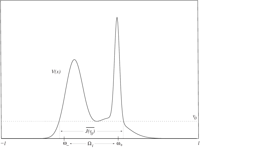
Since we want to focus on shape resonances, we impose a hypothesis that prevents resonances from being produced in the exterior region for energies near . We phrase this hypothesis in terms of a non-trapping condition [3]: We say the potential is non-trapping in at energy (abbreviated is NT), if the following condition is satisfied for :
| (2) |
We assume:
- (H2)
is NT.
Note that formula (2) is equivalent to the more standard virial condition
Furthermore (2) implies the “exterior” virial condition
Our third hypothesis concerns analyticity under exterior dilation. For , we define
We then assume:
- (H3)
defined initially for , has an analytic continuation as a bounded operator to the strip , for some .
For we also define the operators and . It is a straightforward calculation to obtain the associated symbol
Since is a unitary operator on for , we easily compute the domains for the operators and , for :
| (3) |
We define the restrictions of these operators to the box to be
| (4) |
For , is simply the Schrödinger operator described in the introduction that is used to produce plots, such as Figure 1.
The following lemma describes the analytic continuations of these families of operators to complex values of :
Lemma 1
Hypotheses (H1)–(H3) imply the following two conclusions:
- 1.
and are self-adjoint analytic families of Type (A) of m-sectorial operators.
- 2.
and are self-adjoint analytic families of operators.
Proof: These conclusions for the families and are proved in [4]. The same proofs apply for the families and since the proofs in [4] make no use of the (un)boundedness of .
We next recall the Agmon distance [1], that we denote by the symbol . It is the distance associated to the pseudo-metric . We introduce the abbreviations
| and |
The following theorem gives precise information about the resonance on the line and the “resonance in the box.” Its first conclusion follows from [4].
Theorem 2
Assume (H1)–(H3) and that is the eigenvalue of .
- (i)
For any and sufficiently small , there exists , such that has a (complex) eigenvalue close to that satisfies:
- (ii)
The same is true for the operator . Furthermore its eigenvalue is stable in the sense of Kato [7, Sec. VIII.1.4], as the box size tends to infinity. As tends to infinity, this eigenvalue converges to the corresponding eigenvalue of .
- (iii)
For sufficiently small and those values of , for which there exist positive constants and , such that , there exists a real eigenvalue of close to that satisfies the same type of expansion as above.
Remark: (a) Note that in [4], the theorem is stated with replaced by . Due to the possible choices of , the difference between the two quantities can be made arbitrarily small and can be absorbed into . But then, how small must be chosen, depends on .
(b) In the third conclusion of this theorem, one cannot expect uniform results in and . The eigenvalues of the exterior operator have different dependence on and than the eigenvalues of the interior operator . The condition dist is technical; we cannot handle exponentially closely spaced eigenvalues. It is well known that under our hypotheses, the eigenvalues of near the bottom of the well (close to ) cannot be spaced more closely than . Here, the constant is strictly smaller than 2. Its value depends on how flat the bottom of the well is. In order to prove that eigenvalues from do not cause dist to be violated for all , we would need an additional assumption on the decay of the potential. For example, together with dilation analyticity, it would be enough to assume that tends to a limit at infinity like for any .
We now turn our attention to the gaps in the avoided crossings that occur in graphs of the eigenvalues of . For this part of our analysis, we replace hypotheses (H2) and (H3) by the following:
- (H4)
. For , the potential obeys and there exist two constants , such that as tends to . Furthermore for , we have as tends to .
This hypothesis allows us to use WKB estimates to analyze the behavior of eigenvalues of . We note that decomposes into the direct sum of and , where acts on and acts on .
We have the following result on the gaps:
Theorem 3
Assume (H1) and (H4). Suppose is an eigenvalue of and of , but not of . Assume it satisfies , for some positive constants and and . Then we have the following: For fixed values of that are sufficiently small, there exists a neighborhood of , such that for all in , has two eigenvalues and that are exponentially close to . These two eigenvalues are separated by a gap that satisfies
In this estimate, and satisfy the following for any :
| if | |||||||
| if |
Remark: (a) Here, does not depend on .
(b) The width of the resonance is given by the tunneling parameter according to Theorem 2. We do not know whether the resonance is going to tunnel to the left or right, so we only obtain the estimate . In Theorem 3 we know to which side the resonance escapes, and the result is more precise. We also obtain estimates for both of the gap sizes that can occur in the avoided crossings for a given resonance. Since , Theorem 3 shows that the larger gap is of the same order as the square root of the resonance width. We again note that in [8], a radial symmetric situation is studied, so that there is only one way for the resonance to escape, and hence only one gap size.
(c) The eigenvalues of are obviously independent of , but not of . Thus, it might seem that the condition of having a double eigenvalue is crucially dependent on the choice of . This is not case: From Theorem 2 (iii) we see that the eigenvalues of vary only by an exponentially small quantity in when the are varied. For the eigenvalues of , we show in B, that (H4) implies that eigenvalues that belong to an interval are related to , , and a quantum number by the asymptotic formula
We thus have the following consequence: Suppose, for example, that the -th eigenvalue of coincides with an eigenvalue of for some choice of , and that is at least a distance of from the spectrum of . Then for any other choice of , there exists an in a neighborhood of , such that is an eigenvalue of , and the distance from to the spectrum of is still at least .
3 The Proofs
Inspection of the proofs of [4] for Theorem 2 (i) shows that they are valid whether or not is bounded. Furthermore, these proofs can be separated into two parts: The first is a formal algebraic part that shows the stability of the eigenvalue of for the whole operator and constructs the asymptotic expansion of the perturbed eigenvalue in powers of the tunneling parameter . It is quite simple and short. The second part is the justification of these algebraic formulas with the corresponding estimates. This part is more complicated and involves estimation of the operators involved in Krein’s formula.
We present the formal algebraic part, which is needed in all of the situations treated in Theorems 2 (ii), 2 (iii), and Theorem 3. We do this in Section 3.1 in the context of Theorem 2 (iii). In Section 3.2, we treat the stability of the resonance eigenvalue of as the box size tends to infinity. Finally, in Section 3.3 we prove Theorem 3. In the Appendix, we recall Krein’s formula and present the more technical estimates, including the WKB estimates.
We omit the estimates required to prove the existence and the series expansion of the eigenvalue of because they are identical to those in [4].
3.1 Stability and Tunneling Expansion for The Box
We view as a perturbation of . This perturbation involves two Dirichlet conditions. It is most easily approached by way of Krein’s formula, that exhibits the difference of the resolvents of and as a rank two operator.
The norm of this rank two operator is not small. However, because the Dirichlet conditions are imposed inside the classically forbidden region, its norm does not explode in proportion to the inverse of the distance from the spectrum to the spectral parameter in the resolvents. This allows us to choose the parameters in such a way that the resolvent of the resolvent of is small in norm, and we can still use perturbation theory.
The tunneling expansion is based upon a Feshbach type reduction of the eigenvalue equation with respect to the unperturbed eigenprojection. This leads to an implicit equation that we solve by using the Lagrange inversion formula.
3.1.1 Stability
To simplify the notation, we suppress the dependence in many of the formulas. We define
We choose a contour that lies in the resolvent set of and encloses only in . We then choose a point in the intersection of the resolvent sets of and , but outside of . By using the identity
| (5) |
we obtain the following expression for the eigenprojection associated to :
where . By defining
we can formally write the eigenprojection associated to the perturbed eigenvalue as
If we can choose and , such that , then the inverse term in the integral for can be computed by geometric series. Then the eigenprojection is well defined, and by standard arguments, we can deduce the stability of the eigenvalue for .
To see that we can do this, fix any . Let
| (6) |
Note that by hypothesis, , for some , and that we can choose to be as small as any power of .
We define and . Then, formula (5) implies . Thus, the stability follows from the following proposition that we prove in A.1:
Proposition 4
.
3.1.2 Tunneling expansion
Since we have proven the stability of the eigenvalue and constructed , we can write the eigenvalue equation as
We perform a Feshbach type reduction to this equation, with respect to the projections and . We define the “reduced” resolvent
It satisfies the following estimate:
Proposition 5
For any in the disc delimited by , one has .
Proof: If we replace the by in the definition of , we obtain a trivial result. The conclusion to the proposition is obtained by applying perturbation theory to this trivial result.
For the reduction yields the implicit equation
Using properties of the trace and the factorization , c.f. A.1, we obtain
| or equivalently | ||||
| (7) | ||||
where (suppressing in and )
| (8) |
For any in the disc delimited by and , we have the following estimate on :
This follows from Proposition 5 and the bound on , c.f. A.1. If we can establish the estimate of Theorem 2, then equation (7) can be solved with Lagrange’s inversion formula [5, p.250]
Multiplying by and rearranging, we obtain
We estimate the coefficients by using the Cauchy formula
We define and easily obtain the estimate of Theorem 2.
3.1.3 The tunneling parameter
The above calculation relies on the estimate . To prove this, we note that if denotes the eigenfunction associated to , then using the definitions and estimations of A.1,
For each part of Theorem 2, we can estimate the expression by the well known decay estimates of Agmon [1]. This implies the results of Theorem 2.
3.2 Stability as The Box Size Tends to Infinity
We consider the operator
| (9) |
where is the operator defined in (4), and
It is easy to see that is an analytic family of Type (A) in , and that we have the following resolvent estimate:
Proposition 6
Assume (H1)–(H3) and let denote the constant in the non-trapping condition (H2). Let . Then
Proof: decomposes into a direct sum of operators that act on and . We consider only the term associated to the interval ; analogous formulas hold for the other term. We mimic arguments of [3]. For and any , we have
For we use this with to obtain
For negative we repeat this calculation with . This proves the proposition.
We now fix as in [4]. With the definitions of and as in Section 3.1, we define
Here, projects onto the eigenspace for the eigenvalue , but does so in the space . To prove stability of the eigenvalue in the generalized sense (c.f. Kato, [7, Sec. VIII.1.4]), we must show that as tends to , where
It is shown in [4] that for sufficiently small , , uniformly on . The estimates of [4] are also valid for . So, from Proposition 6 and identity (5), we see that,
uniformly on . Thus, we need only show that for any ,
uniformly in . This is shown in A.2
3.3 Proof of Theorem 3
In the degenerate case, we must solve for two eigenvalues. So, we cannot a priori use the Lagrange inversion formula to solve equation (7) in the disc delimited by .
However, we could use the formula if one of the solutions were known to be . This would happen if were a rank one operator. In that case, the spectra of and would intertwine, and as a consequence, at the crossing of two eigenvalues of there would have to be an eigenvalue of .
In our situation such a scenario can be realized by lifting the two Dirichlet conditions one after the other.
It suffices to consider the case where . In the first step, we consider the operators
By hypothesis, is small and fixed, and has the eigenvalue , which for is a distance of from the rest of the spectrum of , i.e. is a simple, conveniently isolated eigenvalue of . Thus, the analog Theorem 2 (iii) is valid:
Lemma 7
Assume the hypotheses of Theorem 3 with . Then there exists a neighborhood of , of size , such that for each , the operator has an eigenvalue close to that satisfies the following for any
Proof: We first note that as we vary , with the restriction that , remains isolated from the rest of the spectrum by a distance of size . Thus, we can prove the lemma by mimicking the proof of Theorem 2 (iii).
For the second step, we note that due to the behavior of there exists an , such that
We now use the intertwining of the spectra of and . We obtain the following lemma by using the techniques we used for Lemma 7 and noting that the eigenfunction associated to has the form , where and :
Lemma 8
Assume H(1) and (H4) and that is a double eigenvalue of as constructed above. Then the operator has two eigenvalues and that satisfy
where, for any ,
| and |
The last step in the proof of Theorem 3 is to note that the first two steps can be done for any admissible . The -th eigenvalue of changes by only an exponentially small amount in when is varied, so it remains properly isolated from . Furthermore, by the behavior of the exterior eigenvalues, there exists an in a neighborhood of , such that the new is also an eigenvalue of . The optimal estimate is obtained when , in which case we have .
Appendix A Krein’s Formula
Since we need Krein’s formula for one and two supplementary Dirichlet boundary conditions, taken at different points depending on the situation, we wish to present the formula in a general setting. On the other hand, for simplicity, we leave out the exterior dilation. We deal with this only when necessary.
Suppose , and are specified. Let and for . Let be a Schrödinger operator on , with self-adjoint boundary conditions at and , and let be the corresponding decoupled operator with supplementary Dirichlet conditions at . Denote their resolvents by and , respectively.
Let and . Define and . Clearly, , and thus, with . We have
We use standard Sobolev space notation and define functionals by the following relations, where :
If for all , we simply write . It is well known that is compact, and consequently, is continuous. Furthermore, Lemma 4 of Section III of [4] shows that whenever satisfies for ,
| (10) |
Finally, we define
With these definitions, we have the following formula,
where all the multiplications are understood to be matrix multiplications.
A.1 Applying Krein’s Formula for Theorem 2 (iii)
In the proof of Theorem 2 (iii), we have , , , ,
Following [4], we define
Since is self-adjoint, we can write
Furthermore, since , we have
We combine the two formulas to obtain
Proposition 4 now follows from
Proposition 9
Let . Fix any . Then for sufficiently small and any ,
Proof: The assertion on is proved in step 5 of the proof of Theorem III.3 of [4]. As for we have
where and . Let be a function supported around such that . Using the estimate (10), it suffices to find a uniform bound on the expressions
We choose , such that for . Then steps 1 and 2 of the proof of Theorem III.3 of [4] show that all theses terms are uniformly bounded.
A.2 Applying Krein’s Formula for Theorem 2 (ii)
Here we consider the difference of the resolvents of the operators defined by formula (3) of the introduction and defined by formula (9). In this case, , , , , and . The difference of the resolvents is
Let be a function supported around , with . To show that and are uniformly bounded operators we use the estimate (10). Thus, it suffices to show that and are uniformly bounded operators from to . If that is true, then for , we have
uniformly in , since .
We now address the required uniform bounds. Commuting and , we need only consider and . The expressions for are analogous and can be treated the same way. The formula
shows that it is sufficient to bound and . We have
For , we set , and then write
The right hand side is uniformly bounded in and by Propostion 6 and Lemma II.3 and Theorem III.3 of [4], which are also valid for and , respectively.
Appendix B WKB Estimates
For these estimates, we follow Olver [9, Ch. 11]. The goal is to find approximate solutions to the differential equation
| (11) |
in with for some positive . Due to either the non-trapping condition or the explicit assumption (H4), there is at most one turning point in each of the intervals and . There is exactly one, if is sufficiently small. We assume has been chosen so that this is the case.
It suffices to consider the interval , and we denote the turning point by . We define a new independent variable by
By integration, we obtain
Note that . It is easy to check that under our conditions, Theorem 3.1 of [9, Ch. 11] shows that equation (11) has two solutions and in , such that
| (12) |
Higher order approximations are also known, c.f. [9, Sec. 11.7].
The Dirichlet boundary conditions imply the quantization condition
Factoring the error in (12) in the classically forbidden region, using the asymptotic expansions of the Airy functions [9, p.392/3], and substituting all this into the quantization condition yields
If this equation is satisfied, then necessarily, . This implies , or equivalently
Now using (H4), we have
From this, it follows that
References
- [1] S. Agmon. Lectures on Exponential Decay of Solutions of Second Order Elliptic Operators. Number 29 in Princeton Mathematical Notes. Princeton University Press, 1982.
- [2] J. Aguilar and J.-M. Combes. A class of analytic perturbations for one-body schrödinger hamiltonians. Commun. Math. Phys., 22:269–279, 1971.
- [3] Philippe Briet, Jean-Michel Combes, and Pierre Duclos. On the location of resonances for Schrödinger operators in the semiclassical limit I: Resonance free domains. J.Math.Anal.Appl., 125:90–99, 1987.
- [4] Jean-Michel Combes, Pierre Duclos, Markus Klein, and Ruedi Seiler. The shape resonance. Commun. Math. Phys., 110:215–236, 1987.
- [5] Jean Dieudonné. Calcul Infinitésimal. Collection Méthodes. Hermann, Paris 1968.
- [6] V.I. Kukulin et al. Theory of Resonances, Principles and Applications. Reidl Texts in the Mathematical Sciences. Kluwer Academic Publishers, 1989.
- [7] Tosio Kato. Pertubation Theory for Linear Operators. Number 132 in Grundlehren der mathematischen Wissenschaften. Springer, Berlin, 3rd edition, 1980.
- [8] C.H. Maier, L.S. Cederbaum, and W. Domcke. A spherical-box approach to resonances. J. Phys. B: Atom. Molec. Phys, 13:L119–L124, 1980.
- [9] F. W. J. Olver. Asymptotics and Special Functions. Computer Science and Applied Mathemetics. Academic Press, New York and London, 1974.
- [10] Michael Reed and Barry Simon. Analysis of Operators, volume IV of Methods of Modern Mathematical Physics. Academic Press, San Diego, 1978.
- [11] Eugene P. Wigner and von Neumann. Über das Verhalten von Eigenwerten bei adiabatischen Prozessen. Zeitschr. f. Phys, 1927.