跳到论文正文
W Papers独立论文阅读器 arXiv:math-ph/0703023 论文正文 计算阅读时间 · 0%
引用这篇论文根据当前论文元数据生成,正式投稿前建议核对。


License: Assumed arXiv.org perpetual non-exclusive license
arXiv:math-ph/0703023v1 [math-ph] 07 Mar 2007

Transition between Airy1 and Airy2 processes and TASEP fluctuationsThanks: Chiba University, e-mail: sasamoto@math.s.chiba-u.ac.jp

Alexei Borodin Thanks: California Institute of Technology, e-mail: borodin@caltech.edu    Patrik L. Ferrari Thanks: Weierstrass Institute (WIAS), Berlin, e-mail: ferrari@wias-berlin.de Affiliation: Tomohiro Sasamoto
March 6, 2007
Abstract

We consider the totally asymmetric simple exclusion process, a model in the KPZ universality class. We focus on the fluctuations of particle positions starting with certain deterministic initial conditions. For large time tt, one has regions with constant and linearly decreasing density. The fluctuations on these two regions are given by the Airy1 and Airy2 processes, whose one-point distributions are the GOE and GUE Tracy-Widom distributions of random matrix theory. In this paper we analyze the transition region between these two regimes and obtain the transition process. Its one-point distribution is a new interpolation between GOE and GUE edge distributions.

1 Introduction

In the search of universal limit distribution functions and limit processes, we consider the KPZ universality class (KPZ for Kardar-Parisi-Zhang) originally introduced for stochastic growth models [13]. For growth in 1+11+1 dimensions the scaling exponents of fluctuations, 1/31/3, and correlations, 2/32/3, can be (non rigorously) determined by some involved arguments, see e.g. [16] for an extended discussion. However, to get more insights into the limit laws and limit processes, one is led to consider solvable models in the universality class.

One such model is the polynuclear growth (PNG) model in discrete time, which has two interesting limits, where new processes have been discovered. The first limit is the continuous time PNG model, for which it has been shown that the surface growing in a droplet shape is, in the large time limit, governed by the Airy2 process [20]. The second one is the totally asymmetric simple exclusion process (TASEP), in which quite recently the limit process of the particles positions starting from a periodic initial conditions has been unravelled and called Airy1 process [21, 2]. In the surface growth picture this corresponds to the flat initial conditions.

If xk​(t)x_{k}(t) denotes the position of particle with label kk, one of the usual geometric representation of the TASEP in terms of surface growth is obtained by the graph {(k,xk​(t)+k)}\{(k,x_{k}(t)+k)\}, see Figure 1 (right) and also e.g. [5]. By universality it is expected that the limit process in one-dimensional KPZ growth is the Airy2 process for the curved regions of the limit shape, and the Airy1 process for the flat parts. However initial conditions can easily generate limit shapes which have both curved and flat regions. Therefore there exist transition regions where the limit shape smoothly changes between curved and flat.

Refer to caption
Figure 1: Left: the density ρ\rho for large time tt is linearly decreasing from (0,1/2)(0,1/2) to (t,0)(t,0). Right: The limit shape in an associated growth, obtained from the density (k∈ℕk\in\mathbbm{N} is the label of the particle which starts at −2​k-2k and xk​(t)x_{k}(t) is its position at time tt).

The novelty of this paper is the analysis of this transition region in the framework of the TASEP. The observables we consider are positions of several particles at time tt. In [10], step-initial conditions (particles starting from ℤ−\mathbbm{Z}_{-}) have been considered from the perspective of a growth model and it was proved that the Airy2 process appears in the large time limit. In [2, 1] we considered periodic initial conditions (particles starting from d​ℤd\mathbbm{Z}, d=2,3,…d=2,3,\ldots) and obtained the Airy1 process as the limit process.

To obtain both regimes and the transition region, we consider in this paper particles starting from 2​ℤ−2\mathbbm{Z}_{-} as in [21]. There are four regions of interest as illustrated in Figure 1 (left).
(1) Constant density region. The limit process of particle positions is given by the Airy1 process 𝒜1{\cal A}_{\rm 1}. In particular, the one-point distribution is F1​(22/3​s)F_{1}(2^{2/3}s), with F1F_{1} being the GOE Tracy-Widom distribution.
(2) Linearly decreasing density region. The limit process is the Airy2 process 𝒜2{\cal A}_{\rm 2}, which has F2​(s)F_{2}(s) as one-point distribution, with F2F_{2} being the GUE Tracy-Widom distribution.
(3) Finite distance from the right-most particle. There the particle positions are described via the GUE-minor kernel [12]. In particular, the nn-th right-most particle is distributed as the largest eigenvalue of the nn-particle GUE ensemble.
(4) The transition region between (1) and (2). The fluctuations are governed by a new process obtained in this paper: the transition process Airy2→1, which we denote 𝒜2→1{\cal A}_{2\to 1}. In particular, the one-point distribution interpolates between F2​(s)F_{2}(s) and F1​(22/3​s)F_{1}(2^{2/3}s) and the transition region has width which scales in time as t2/3t^{2/3}.

The analysis is done by using the framework of signed determinantal point processes introduced in [2]. This new approach allows us to analyze all four regions for our initial conditions. This is contrasted to the previously used determinantal point process issued by the RSK construction, by which only the step initial condition or its variants could be analyzed [10, 22, 8, 9, 4, 6, 20, 3]. We explain how the analysis has to be done for all 4 cases, but the complete asymptotic analysis is presented only for the transition region, the technically most difficult one, and the really new result of this paper. The result is a process, 𝒜2→1{\cal A}_{2\to 1}, interpolating between the Airy2 and the Airy1 processes. For more details about the Airy processes, see the review [5].

The transition we discovered is not the first one between some GUE and GOE type distributions, but it seems to be different from the one previously known for random matrices, non-colliding Brownian motions with open boundary condition and so on [7, 14, 19, 22]. The main differences are the following. On the natural scale of the problems considered, the final distribution is F1​(22/3​s)F_{1}(2^{2/3}s) for our case and F1​(s)F_{1}(s) in the previous case. Secondly, in the previous case, the GOE-type distribution appears at a single point, while in our case, the GOE-type distribution is on an extended region. Moreover, our transition smoothly interpolates between F2​(s)F_{2}(s) and F1​(22/3​s)F_{1}(2^{2/3}s), which is not the case for the other transition. In principle, we can not however yet exclude that by a change of variable, with both the rescaling of fluctuations and spatial correlations, the two transitions map one to the other.

Outline. In Section 2 we define the model we analyze and state the results. In Section 3 we explain the finite time result and set the scaling limit. In Section 4 we do the complete asymptotic analysis for the transition region and in Section 5 we explain how to do the analysis for the other cases. Finally, we present an explicit form of the transition kernel in terms of Airy functions in Appendix A and we explain the correctness of the Fredholm determinants involved in B.

Acknowledgments

A. Borodin was partially supported by the NSF grant DMS-0402047 and the CRDF grant RIM1-2622-ST-04. P.L. Ferrari would like to thank for the support of the German-Japanese cooperation project of German National Foundation, DFG 446JAP113/325/0-1. The work of T. Sasamoto is supported by the Grant-in-Aid for Young Scientists (B), the Ministry of Education, Culture, Sports, Science and Technology, Japan.

2 Model and results

In this paper we consider the continuous-time totally asymmetric simple exclusion process (TASEP) on ℤ\mathbbm{Z}. At any given time tt, every site j∈ℤj\in\mathbbm{Z} can be occupied at most by one particle. Thus a configuration of the TASEP can be described by η={ηj,j∈ℤ|ηj∈{0,1}}∈Ω={0,1}ℤ\eta=\{\eta_{j},j\in\mathbbm{Z}|\eta_{j}\in\{0,1\}\}\in\Omega=\{0,1\}^{\mathbbm{Z}}. ηj\eta_{j} is called the occupation variable of site jj, which is defined by ηj=1\eta_{j}=1 if site jj is occupied and ηj=0\eta_{j}=0 if site jj is empty.

The dynamics of the TASEP is defined as follows. Particles jump on the neighboring right site with rate 11 provided that the site is empty. This means that jumps are independent of each other and are performed after an exponential waiting time with mean 11. More precisely, let ff: Ω→ℝ\Omega\to\mathbbm{R} be a function depending only on a finite number of ηj\eta_{j}’s. Then the backward generator of the TASEP is given by

L​f​(η)=∑j∈ℤηj​(1−ηj+1)​(f⁡(ηj,j+1)−f⁡(η)).Lf(\eta)=\sum_{j\in\mathbbm{Z}}\eta_{j}(1-\eta_{j+1})\big(f(\eta^{j,j+1})-f(\eta)\big). (2.1)

Here ηj,j+1\eta^{j,j+1} denotes the configuration η\eta with the occupations at sites jj and j+1j+1 interchanged. The semigroup eL​te^{Lt} is well-defined as acting on bounded and continuous functions on Ω\Omega. eL​te^{Lt} is the transition probability of the TASEP [18].

We denote by xk​(t)x_{k}(t) the position of the particle number kk at time tt. As initial condition we consider particles starting from 2​ℤ−2\mathbbm{Z}_{-}, i.e., xk​(0)=−2​kx_{k}(0)=-2k for k=1,2,…k=1,2,\ldots. On the macroscopic level, the limit particle density u⁡(ξ)u(\xi) is given by

u(ξ)=dd​ξlimt→∞1t𝔼(#(k:xk(t)≥ξt))={1/2,ξ<0,1/2−ξ/2,ξ∈[0,1],0,ξ>1.u(\xi)=\frac{\mathrm{d}}{\mathrm{d}\xi}\lim_{t\to\infty}\frac{1}{t}\mathbb{E}\big(\#(k:x_{k}(t)\geq\xi t)\big)=\left\{\begin{array}[]{ll}1/2,&\xi<0,\\ 1/2-\xi/2,&\xi\in[0,1],\\ 0,&\xi>1.\end{array}\right. (2.2)

Thus for large time tt the expected number of particle at site xx, ρ⁡(x)\rho(x), is close to u⁡(x/t)u(x/t), see Figure 1.

As observables we consider the positions of finite subsets of particles, {xi​(t),i∈I}\{x_{i}(t),i\in I\} for some I⊂ℕI\subset\mathbbm{N}, |I|<∞|I|<\infty. The scaling limits we have to take depend on which of the four regions described in the Introduction we focus on, see also Figure 1. The main result of this paper is the description of the large time fluctuations in the transition region, which now we describe.

(4) Transition region: the 𝒜2→1{\cal A}_{2\to 1} process

The transition region has width of order t2/3t^{2/3}, which is indicated by the fact that the index of the particles which at time tt are around x=0x=0 fluctuates on the t2/3t^{2/3} scale around the macroscopic value t/4t/4. Therefore we set

n⁡(τ,t)=[t/4+τ​(t/2)2/3].n(\tau,t)=[t/4+\tau(t/2)^{2/3}]. (2.3)

The density (2.2) changes in the transition region. The limit density can be used to determine, on the macroscopic scale, the expected location at time tt of a particle with index n⁡(a)=[t/4+a​t]n(a)=[t/4+at] (of course a≥−1/4a\geq-1/4). The result is then

limt→∞xn⁡(a)t={1−1+4​a,a∈[−1/4,0],−2​a,a≥0.\lim_{t\to\infty}\frac{x_{n(a)}}{t}=\left\{\begin{array}[]{ll}1-\sqrt{1+4a},&a\in[-1/4,0],\\ -2a,&a\geq 0.\end{array}\right. (2.4)

By using (2.4) with a​t=τ​(t/2)2/3at=\tau(t/2)^{2/3} we are led to define the rescaled process of particle positions by

τ↦Xt​(τ)=xn⁡(τ,t)​(t)−(−2​τ​(t/2)2/3+min⁡{0,τ}2​(t/2)1/3)−(t/2)1/3.\tau\mapsto X_{t}(\tau)=\frac{x_{n(\tau,t)}(t)-(-2\tau(t/2)^{2/3}+\min\{0,\tau\}^{2}(t/2)^{1/3})}{-(t/2)^{1/3}}. (2.5)

The main result of this paper is the convergence of Xt​(τ)X_{t}(\tau) to the transition process 𝒜2→1{\cal A}_{2\to 1} defined below.

Definition 1 (The Airy2→1 process).

Let us set

s~i={si,τi≥0,si−τi2,τi≤0.\tilde{s}_{i}=\left\{\begin{array}[]{ll}s_{i},&\tau_{i}\geq 0,\\ s_{i}-\tau_{i}^{2},&\tau_{i}\leq 0.\end{array}\right. (2.6)

and define the transition kernel

K∞​(τ1,s1,τ2,s2)=−14​π​(τ2−τ1)​exp⁡(−(s~2−s~1)24​(τ2−τ1))​𝟙​(τ2>τ1)\displaystyle K_{\infty}(\tau_{1},s_{1};\tau_{2},s_{2})=-\frac{1}{\sqrt{4\pi(\tau_{2}-\tau_{1})}}\exp\left(-\frac{(\tilde{s}_{2}-\tilde{s}_{1})^{2}}{4(\tau_{2}-\tau_{1})}\right)\mathbbm{1}(\tau_{2}>\tau_{1})
+1(2​π​i)2∫γ+dw∫γ−dzew3/3+τ2​w2−s~2​wez3/3+τ1​z2−s~1​z2​w(z−w)​(z+w)\displaystyle+\frac{1}{(2\pi{\rm i})^{2}}\int_{\gamma_{+}}\mathrm{d}w\int_{\gamma_{-}}\mathrm{d}z\frac{e^{w^{3}/3+\tau_{2}w^{2}-\tilde{s}_{2}w}}{e^{z^{3}/3+\tau_{1}z^{2}-\tilde{s}_{1}z}}\frac{2w}{(z-w)(z+w)} (2.7)

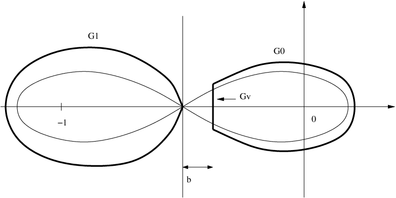
with the paths γ+,γ−\gamma_{+},\gamma_{-} satisfying −γ+⊂γ−-\gamma_{+}\subset\gamma_{-} with γ+:ei​ϕ+​∞→e−i​ϕ+​∞\gamma_{+}:e^{{\rm i}\phi_{+}}\infty\to e^{-{\rm i}\phi_{+}}\infty, γ−:e−i​ϕ−​∞→ei​ϕ−​∞\gamma_{-}:e^{-{\rm i}\phi_{-}}\infty\to e^{{\rm i}\phi_{-}}\infty for some ϕ+∈(π/3,π/2)\phi_{+}\in(\pi/3,\pi/2), ϕ−∈(π/2,π−ϕ+)\phi_{-}\in(\pi/2,\pi-\phi_{+}), see Figure 2.

Refer to caption
Figure 2: An illustration of the paths γ+\gamma_{+} and γ−\gamma_{-} in Definition 1.

The Airy2→1 process, 𝒜2→1{\cal A}_{2\to 1}, is the process with mm-point joint distributions at τ1<τ2<…<τm\tau_{1}<\tau_{2}<\ldots<\tau_{m} given by the Fredholm determinant

ℙ(⋂k=1m{𝒜2→1(τk)≤sk})=det(𝟙−χsK∞χs)L2​({τ1,…,τm}×ℝ)\mathbbm{P}\bigg(\bigcap_{k=1}^{m}\{{\cal A}_{2\to 1}(\tau_{k})\leq s_{k}\}\bigg)=\det(\mathbbm{1}-\chi_{s}K_{\infty}\chi_{s})_{L^{2}(\{\tau_{1},\ldots,\tau_{m}\}\times\mathbbm{R})} (2.8)

where χs​(τk,x)=𝟙​(x>sk)\chi_{s}(\tau_{k},x)=\mathbbm{1}(x>s_{k}). An explicit expression for K∞K_{\infty} in terms of Airy functions can be found in Appendix A.

Remarks: 𝒜2→1​(t+τ){\cal A}_{2\to 1}(t+\tau) becomes 2−1/3𝒜1(22/3τ)2^{-1/3}{\cal A}_{\rm 1}(2^{2/3}\tau) as t→∞t\to\infty and 𝒜2​(τ){\cal A}_{\rm 2}(\tau) when t→−∞t\to-\infty. The Fredholm determinant in (2.8) is well defined because, as proven in Proposition 9 of Appendix B, there exists a conjugate kernel of χs​K∞​χs\chi_{s}K_{\infty}\chi_{s} which is trace-class on ℋ=L2​({τ1,…,τm}×ℝ){\cal H}=L^{2}(\{\tau_{1},\ldots,\tau_{m}\}\times\mathbbm{R}).

Now we can state precisely our main Theorem.

Theorem 2.

The convergence of XtX_{t} to the transition process 𝒜2→1{\cal A}_{2\to 1},

limt→∞Xt​(τ)=𝒜2→1​(τ),\lim_{t\to\infty}X_{t}(\tau)={\cal A}_{2\to 1}(\tau), (2.9)

holds in the sense of finite-dimensional distributions.

A remark on initial conditions. In this work as well as in many of the previous papers in the field, the situations analyzed with deterministic initial conditions might look quite peculiar: step-initial conditions [11], periodic with period 22 or more [2, 1]. However, it is intuitively clear that small perturbations of the initial conditions do not affect the large time behavior. This is indeed the case by a coupling argument.

Consider two TASEP initial conditions of NN particles, X(0)={xN(0)<…<x2(0)<x1(0)}X(0)=\{x_{N}(0)<\ldots<x_{2}(0)<x_{1}(0)\}, Z(0)={zN(0)<…<z2(0)<z1(0)}Z(0)=\{z_{N}(0)<\ldots<z_{2}(0)<z_{1}(0)\} with X⁡(0)≤Z⁡(0)X(0)\leq Z(0) meaning xk​(0)≤zk​(0)x_{k}(0)\leq z_{k}(0), k=1,…,Nk=1,\ldots,N. By a standard coupling argument, see e.g. [17], for any subset I⊂{1,…,N}I\subset\{1,\ldots,N\},

ℙ⁡({xi​(t)≤ai,i∈I})≥ℙ⁡({zi​(t)≤ai,i∈I}).\mathbbm{P}(\{x_{i}(t)\leq a_{i},i\in I\})\geq\mathbbm{P}(\{z_{i}(t)\leq a_{i},i\in I\}). (2.10)

We can apply (2.10) to our case to show that the limit result is unchanged if we do any bounded perturbation of the initial condition. In Theorem 2 we started with initial conditions xi​(0)=−2​ix_{i}(0)=-2i. Consider any other initial condition Z={zi​(0)}Z=\{z_{i}(0)\} and define

M=max⁡{|xi​(0)−zi​(0)|}.M=\max\{|x_{i}(0)-z_{i}(0)|\}. (2.11)

Then, by (2.10), we have

ℙ⁡({xi​(t)≤ai+M,i∈I})\displaystyle\mathbbm{P}(\{x_{i}(t)\leq a_{i}+M,i\in I\}) ≥\displaystyle\geq ℙ⁡({zi​(t)≤ai,i∈I})\displaystyle\mathbbm{P}(\{z_{i}(t)\leq a_{i},i\in I\}) (2.12)
≥\displaystyle\geq ℙ⁡({xi​(t)≤ai−M,i∈I}).\displaystyle\mathbbm{P}(\{x_{i}(t)\leq a_{i}-M,i\in I\}).

In the scaling limit (2.5), the first and last term in (2.12) have the same limit as t→∞t\to\infty as long as limt→∞M/t1/3=0\lim_{t\to\infty}M/t^{1/3}=0. This holds in particular if ZZ is any bounded perturbation of XX, i.e., if M<∞M<\infty is independent of tt.

For completeness we state the results in the other three regions. In Section 5 we outline how the asymptotic analysis for the transition region has to be modified in order to obtain the results. The scaling is obtained using (2.4).

(1) Fixed particle number: GUE​(n)\textrm{GUE}(n) minors

Consider particles with index not rescaled in time, i.e.,

n​ of order one,n\text{ of order one}, (2.13)

and the rescaled random variables

Xt​(n)=xn​(t)−t−2​t.X_{t}(n)=\frac{x_{n}(t)-t}{-\sqrt{2t}}. (2.14)

Then, in the t→∞t\to\infty limit, one gets the GUE-minors​(n)\textrm{GUE-minors}(n) given in [12],

limt→∞Xt​(n)=GUE-minors​(n).\lim_{t\to\infty}X_{t}(n)=\textrm{GUE-minors}(n). (2.15)

(2) Linearly decreasing density region: Airy2 process, 𝒜2{\cal A}_{\rm 2}

For 0<α<10<\alpha<1, define

n⁡(τ,t)=[α​t/4+τ​(t/2)2/3],n(\tau,t)=[\alpha t/4+\tau(t/2)^{2/3}], (2.16)

and the rescaled process

τ↦Xt​(τ)=xn⁡(τ,t)(t)−((1−α)t−2τα−1/2(t/2)2/3+τ2α−3/2(t/2)1/3)−(t/2)1/3.\tau\mapsto X_{t}(\tau)=\frac{x_{n(\tau,t)}(t)-((1-\sqrt{\alpha})t-2\tau\alpha^{-1/2}(t/2)^{2/3}+\tau^{2}\alpha^{-3/2}(t/2)^{1/3})}{-(t/2)^{1/3}}. (2.17)

Then in the t→∞t\to\infty limit, one gets

limt→∞Xt​(τ)=(2−α)2/3α1/6​𝒜2​(τ​α2/3​(2−α)1/3).\lim_{t\to\infty}X_{t}(\tau)=\frac{(2-\sqrt{\alpha})^{2/3}}{\alpha^{1/6}}{\cal A}_{\rm 2}(\tau\alpha^{2/3}(2-\sqrt{\alpha})^{1/3}). (2.18)

(3) Constant density region: Airy1 process, 𝒜1{\cal A}_{\rm 1}

For α>1\alpha>1,

n⁡(τ,t)=[α​t/4+τ​(t/2)2/3],n(\tau,t)=[\alpha t/4+\tau(t/2)^{2/3}], (2.19)

and the rescaled process variables

τ↦Xt​(τ)=xn⁡(τ,t)​(t)−((1−α)​t/2−2​τ​(t/2)2/3)−(t/2)1/3.\tau\mapsto X_{t}(\tau)=\frac{x_{n(\tau,t)}(t)-((1-\alpha)t/2-2\tau(t/2)^{2/3})}{-(t/2)^{1/3}}. (2.20)

Then in the t→∞t\to\infty limit, one gets

limt→∞Xt​(τ)=21/3​𝒜1​(22/3​τ).\lim_{t\to\infty}X_{t}(\tau)=2^{1/3}{\cal A}_{\rm 1}(2^{2/3}\tau). (2.21)

3 Kernel and its scaling limit

In this section we derive the expression of the joint distributions of particle positions and then set the proper scaling limit.

Consider NN particles starting at time t=0t=0 at positions xk​(0)=−2​kx_{k}(0)=-2k, k=1,…,Nk=1,\ldots,N. In Theorem 2.1 of [2] we proved that the joint distribution of the positions of the particles are given by a Fredholm determinant. The kernel is determined via a certain orthogonalization, which for our initial conditions has been made in Lemma 4.1 of [2] (with z=x+2​n−2​Nz=x+2n-2N replaced by z=x+2​nz=x+2n). Once the orthogonalization is made, one can compute the kernel which is (4.11) of [2] (with zi=xi+2​ni−2​Nz_{i}=x_{i}+2n_{i}-2N replaced by zi=xi+2​niz_{i}=x_{i}+2n_{i}). This is summarized in Proposition 3.

Proposition 3.

Let particle with label ii start at xi​(0)=−2​ix_{i}(0)=-2i, i=1,…,Ni=1,\ldots,N. At time tt, the particles are at positions xix_{i}. Let σ⁡(1)<σ⁡(2)<…<σ⁡(m)\sigma(1)<\sigma(2)<\ldots<\sigma(m) be the indices of mm out of the NN particles. The joint distribution of their positions xσ⁡(k)​(t)x_{\sigma(k)}(t) is given by

ℙ(⋂k=1m{xσ⁡(k)(t)≥ak})=det(𝟙−χaKtχa)ℓ2​({σ⁡(1),…,σ⁡(m)}×ℤ)\mathbbm{P}\Big(\bigcap_{k=1}^{m}\big\{x_{\sigma(k)}(t)\geq a_{k}\big\}\Big)=\det(\mathbbm{1}-\chi_{a}K_{t}\chi_{a})_{\ell^{2}(\{\sigma(1),\ldots,\sigma(m)\}\times\mathbbm{Z})} (3.1)

where χa​(σ⁡(k),x)=𝟙​(x<ak)\chi_{a}(\sigma(k),x)=\mathbbm{1}(x<a_{k}). The kernel KtK_{t} is given by

Kt(n1,x1;n2,x2)=−(x1−x2−1n2−n1−1)𝟙[n2>n1]+K^t(n1,x1;n2,x2),K_{t}(n_{1},x_{1};n_{2},x_{2})=-\binom{x_{1}-x_{2}-1}{n_{2}-n_{1}-1}\mathbbm{1}_{[n_{2}>n_{1}]}+\widehat{K}_{t}(n_{1},x_{1};n_{2},x_{2}), (3.2)

where

K^t​(n1,x1,n2,x2)\displaystyle\widehat{K}_{t}(n_{1},x_{1};n_{2},x_{2}) =\displaystyle= (−1)n1−n2(2​π​i)2​∮Γ0d​v​∮Γ−1d​u​e−v​t​(1+v)x2+n2vn2\displaystyle\frac{(-1)^{n_{1}-n_{2}}}{(2\pi{\rm i})^{2}}\oint_{\Gamma_{0}}\mathrm{d}v\oint_{\Gamma_{-1}}\mathrm{d}u\frac{e^{-vt}(1+v)^{x_{2}+n_{2}}}{v^{n_{2}}} (3.3)
eu​t​un1(1+u)x1+n1+1​1+2​v(u−v)​(1+u+v)\displaystyle\frac{e^{ut}u^{n_{1}}}{(1+u)^{x_{1}+n_{1}+1}}\frac{1+2v}{(u-v)(1+u+v)}

where Γ0\Gamma_{0}, resp. Γ−1\Gamma_{-1}, is any simple loop, anticlockwise oriented, which includes the pole at v=0v=0, resp. u=−1u=-1, satisfying −1−Γ0⊂Γ−1-1-\Gamma_{0}\subset\Gamma_{-1}, i.e., all the points of −1−Γ0-1-\Gamma_{0} lie inside the loop Γ−1\Gamma_{-1}.

In order to prove Theorem 2, we need to focus at particles with number nin_{i} close to t/4t/4 since these particles will be in the transition region at time tt. The transition region has width which scales as t2/3t^{2/3}. The limit density is constant to the left of the transition region and it is decreasing linearly to the right of it. Therefore, the scaling limit used to prove the main theorem is

ni\displaystyle n_{i} =\displaystyle= [t/4+τi​(t/2)2/3],\displaystyle[t/4+\tau_{i}(t/2)^{2/3}],
xi\displaystyle x_{i} =\displaystyle= [−2​τi​(t/2)2/3−s~i​(t/2)1/3],\displaystyle[-2\tau_{i}(t/2)^{2/3}-\tilde{s}_{i}(t/2)^{1/3}], (3.4)

where

s~i={si,τi≥0,si−τi2,τi≤0.\tilde{s}_{i}=\left\{\begin{array}[]{ll}s_{i},&\tau_{i}\geq 0,\\ s_{i}-\tau_{i}^{2},&\tau_{i}\leq 0.\end{array}\right. (3.5)

As a consequence the rescaled kernel writes

Ktresc​(τ1,s1,τ2,s2)=Kt​(n1,x1,n2,x2)​(t/2)1/3​2x2−x1K_{t}^{\rm resc}(\tau_{1},s_{1};\tau_{2},s_{2})=K_{t}(n_{1},x_{1};n_{2},x_{2})(t/2)^{1/3}2^{x_{2}-x_{1}} (3.6)

where 2x2−x12^{x_{2}-x_{1}} is just a conjugation so that the kernel has a proper limit. We denote by K^tresc\widehat{K}_{t}^{\rm resc} the term of the rescaled kernel without the binomial contribution, which then writes

K^tresc​(τ1,s1,τ2,s2)=(t/2)1/3​1(2​π​i)2​∮Γ0d​v​∮Γ−1d​u​1+2​v(u−v)​(1+u+v)\displaystyle\widehat{K}_{t}^{\rm resc}(\tau_{1},s_{1};\tau_{2},s_{2})=(t/2)^{1/3}\frac{1}{(2\pi{\rm i})^{2}}\oint_{\Gamma_{0}}\mathrm{d}v\oint_{\Gamma_{-1}}\mathrm{d}u\frac{1+2v}{(u-v)(1+u+v)}
×exp⁡(t​f0​(v)+(t/2)2/3​τ2​f1​(v)+(t/2)1/3​s~2​f2​(v))exp⁡(t​f0​(u)+(t/2)2/3​τ1​f1​(u)+(t/2)1/3​s~1​f2​(u)+f3​(u)),\displaystyle\times\frac{\exp(tf_{0}(v)+(t/2)^{2/3}\tau_{2}f_{1}(v)+(t/2)^{1/3}\tilde{s}_{2}f_{2}(v))}{\exp(tf_{0}(u)+(t/2)^{2/3}\tau_{1}f_{1}(u)+(t/2)^{1/3}\tilde{s}_{1}f_{2}(u)+f_{3}(u))}, (3.7)

where the functions fif_{i} are given by

f0​(v)\displaystyle f_{0}(v) =\displaystyle= −v+14​ln⁡((1+v)/v),\displaystyle-v+\tfrac{1}{4}\ln((1+v)/v),
f1​(v)\displaystyle f_{1}(v) =\displaystyle= −ln⁡(−4​v​(1+v)),\displaystyle-\ln(-4v(1+v)),
f2​(v)\displaystyle f_{2}(v) =\displaystyle= −ln⁡(2​(1+v)),\displaystyle-\ln(2(1+v)),
f3​(v)\displaystyle f_{3}(v) =\displaystyle= ln⁡(1+v).\displaystyle\ln(1+v). (3.8)

From now on the τi\tau_{i}’s are some fixed values. With this preparation we can proceed to the asymptotic analysis needed to prove Theorem 2.

4 Asymptotic analysis

Proof of Theorem 2. The proof of Theorem 2 is identical to the one of Theorem 2.5 in [1], provided the following Propositions 4, 5, 6, 7, and 8 (convergence on bounded sets and large deviations bounds) hold. ∎

Proposition 4 (Uniform convergence on bounded sets).

Fix any L>0L>0 and xi,six_{i},s_{i} with the scaling (3). Then, uniformly for (s1,s2)∈[−L,L]2(s_{1},s_{2})\in[-L,L]^{2},

limt→∞K^tresc​(n1,x1,n2,x2)=K^∞resc​(τ1,s1,τ2,s2)\lim_{t\to\infty}\widehat{K}_{t}^{\rm resc}(n_{1},x_{1};n_{2},x_{2})=\widehat{K}_{\infty}^{\rm resc}(\tau_{1},s_{1};\tau_{2},s_{2}) (4.1)

where

K^∞​(τ1,s1,τ2,s2)=1(2​π​i)2​∫γ+d​w​∫γ−d​z​ew3/3+τ2​w2−s~2​wez3/3+τ1​z2−s~1​z​2​w(z−w)​(z+w)\widehat{K}_{\infty}(\tau_{1},s_{1};\tau_{2},s_{2})=\frac{1}{(2\pi{\rm i})^{2}}\int_{\gamma_{+}}\mathrm{d}w\int_{\gamma_{-}}\mathrm{d}z\frac{e^{w^{3}/3+\tau_{2}w^{2}-\tilde{s}_{2}w}}{e^{z^{3}/3+\tau_{1}z^{2}-\tilde{s}_{1}z}}\frac{2w}{(z-w)(z+w)} (4.2)

with the paths γ+,γ−\gamma_{+},\gamma_{-} satisfying −γ+⊂γ−-\gamma_{+}\subset\gamma_{-} with γ+:ei​ϕ+​∞→e−i​ϕ+​∞\gamma_{+}:e^{{\rm i}\phi_{+}}\infty\to e^{-{\rm i}\phi_{+}}\infty, γ−:e−i​ϕ−​∞→ei​ϕ−​∞\gamma_{-}:e^{-{\rm i}\phi_{-}}\infty\to e^{{\rm i}\phi_{-}}\infty for some ϕ+∈(π/3,π/2)\phi_{+}\in(\pi/3,\pi/2), ϕ−∈(π/2,π−ϕ+)\phi_{-}\in(\pi/2,\pi-\phi_{+}).

Proof.

The first step is to control the contribution away from the critical point given by

d​f0​(v)d​v=−(1+2​v)24​v​(1+v)=0⇔v=−1/2.\frac{\mathrm{d}f_{0}(v)}{\mathrm{d}v}=-\frac{(1+2v)^{2}}{4v(1+v)}=0\quad\iff\quad v=-1/2. (4.3)

If we write v=x+i​yv=x+{\rm i}y, x,y∈ℝx,y\in\mathbbm{R}, then we can analyze

Re(f0(v)−f0(−1/2))=−(x+1/2)+18ln(((1+x)2+y2)/(x2+y2)).\mathrm{Re}(f_{0}(v)-f_{0}(-1/2))=-(x+1/2)+\tfrac{1}{8}\ln(((1+x)^{2}+y^{2})/(x^{2}+y^{2})). (4.4)

This expression equals zero for
a) x=−1/2x=-1/2, y∈ℝy\in\mathbbm{R},
b) y=±g⁡(x)y=\pm g(x), with g⁡(x)=1+2​x+x2​(1−e8​x+4)e8​x+4−1g(x)=\sqrt{\frac{1+2x+x^{2}(1-e^{8x+4})}{e^{8x+4}-1}}.
If is easy to see that the solutions ±g⁡(x)\pm g(x) are symmetric with respect to v=−1/2v=-1/2 and they go around −1-1 and 00 once. Moreover, the loops leave the critical point v=−1/2v=-1/2 in the directions e±iπ/6e^{\pm{\rm i}\pi/6} and e±i5π/6e^{\pm{\rm i}5\pi/6}, see Figure 3.

Refer to caption
Figure 3: The signum of Re(f0(x+iy)−f0(−1/2))\mathrm{Re}(f_{0}(x+{\rm i}y)-f_{0}(-1/2)) is positive in D2D_{2} and D4D_{4} and negative in D1D_{1} and D3D_{3}.

We denote by D1,…,D4D_{1},\ldots,D_{4} the following regions: D1D_{1} is the region enclosed by ±g\pm g around −1-1, D2D_{2} is the rest with real part less than −1/2-1/2, D4D_{4} is the symmetric image w.r.t. −1/2-1/2 of D1D_{1} and D3D_{3} of D2D_{2}, see Figure 3. Then Γ0\Gamma_{0} can be chosen to be any simple anticlockwise oriented finite length path staying in D3D_{3} and, similarly, Γ−1\Gamma_{-1} is chosen to stay in D2D_{2} (except at v=−1/2v=-1/2). The constraint −1−Γ0⊂Γ−1-1-\Gamma_{0}\subset\Gamma_{-1} is easily satisfied except that for Γ0\Gamma_{0} we have to go through D4D_{4} too, very close to v=−1/2v=-1/2. Moreover, we can take Γ0\Gamma_{0} leaving from −1/2-1/2 with an angle between −π/6-\pi/6 and −π/3-\pi/3. Similarly, Γ−1\Gamma_{-1} leaves in the direction from 2​π/32\pi/3 and 5​π/65\pi/6. This will simplify the argument for moderate and large deviations.

Refer to caption
Figure 4: The paths Γ0\Gamma_{0} and Γ−1\Gamma_{-1} close to the critical point −1/2-1/2. The dashed lines are the zeros of Re(f0(x+iy)−f0(−1/2))\mathrm{Re}(f_{0}(x+{\rm i}y)-f_{0}(-1/2)).

Let us set Γ0δ={v∈Γ0,|v+1/2|≤δ}\Gamma_{0}^{\delta}=\{v\in\Gamma_{0},|v+1/2|\leq\delta\} and Γ−1δ={u∈Γ−1,|u+1/2|≤δ}\Gamma_{-1}^{\delta}=\{u\in\Gamma_{-1},|u+1/2|\leq\delta\}. Then the integral is over Γ0∪Γ−1=Γ0δ∪Γ−1δ+Σ\Gamma_{0}\cup\Gamma_{-1}=\Gamma_{0}^{\delta}\cup\Gamma_{-1}^{\delta}+\Sigma, where Σ\Sigma is the rest of the contours. The first step is to bound the integral over Σ\Sigma. For 0<δ≪10<\delta\ll 1, we can choose Γ0\Gamma_{0} and Γ−1\Gamma_{-1} such that, for (u,v)∈Σ(u,v)\in\Sigma, |u−v|/δ|u-v|/\delta and |1+u+v|/δ|1+u+v|/\delta are bounded away from 00. Then, on Σ\Sigma, |1+2​v(u−v)​(1+u+v)|≤|u−v|−1+|1+u+v|−1=𝒪⁡(1/δ)\left|\frac{1+2v}{(u-v)(1+u+v)}\right|\leq|u-v|^{-1}+|1+u+v|^{-1}=\mathcal{O}(1/\delta) and, for some c0=c0​(δ)>0c_{0}=c_{0}(\delta)>0, Re(f0(v)−f0(−1/2))≤−c0\mathrm{Re}(f_{0}(v)-f_{0}(-1/2))\leq-c_{0} and/or −Re(f0(u)−f0(−1/2))≤−c0-\mathrm{Re}(f_{0}(u)-f_{0}(-1/2))\leq-c_{0}. Thus, the integral over Σ\Sigma can be bounded as

c1​δ−1​t1/3​exp⁡(−c0​t+𝒪⁡(t2/3))c_{1}\delta^{-1}t^{1/3}\exp(-c_{0}t+\mathcal{O}(t^{2/3})) (4.5)

for some c1>0c_{1}>0. For tt large enough, both e𝒪⁡(t2/3)e^{\mathcal{O}(t^{2/3})} and c1​t1/3c_{1}t^{1/3} are bounded by e−c0t/4e^{-c_{0}t/4}. Thus, for tt large enough, we have the bound

|∬Σ⋯|≤δ−1e−c0t/2.\left|\iint_{\Sigma}\cdots\right|\leq\delta^{-1}e^{-c_{0}t/2}. (4.6)

The second step is to control the integral over Γ0δ∪Γ−1δ\Gamma_{0}^{\delta}\cup\Gamma_{-1}^{\delta}. Since δ\delta is small, we can apply Taylor series expansion on the functions fif_{i} defined in (3). For this we change variables by setting

u=−1/2+U,v=−1/2+Vu=-1/2+U,\quad v=-1/2+V (4.7)

and we denote γ+δ=Γ0δ+1/2\gamma_{+}^{\delta}=\Gamma_{0}^{\delta}+1/2, γ−δ=Γ−1δ+1/2\gamma_{-}^{\delta}=\Gamma_{-1}^{\delta}+1/2. We have

f0\displaystyle f_{0} =\displaystyle= 12+i​π4+43​V3+𝒪⁡(V4),\displaystyle\tfrac{1}{2}+{\rm i}\tfrac{\pi}{4}+\tfrac{4}{3}V^{3}+\mathcal{O}(V^{4}),
f1\displaystyle f_{1} =\displaystyle= 4​V2+𝒪⁡(V4),\displaystyle 4V^{2}+\mathcal{O}(V^{4}),
f2\displaystyle f_{2} =\displaystyle= −2​V+𝒪⁡(V2),\displaystyle-2V+\mathcal{O}(V^{2}),
f3\displaystyle f_{3} =\displaystyle= −ln⁡(2)+𝒪⁡(V).\displaystyle-\ln(2)+\mathcal{O}(V). (4.8)

Therefore the integral over Γ0δ∪Γ−1δ\Gamma_{0}^{\delta}\cup\Gamma_{-1}^{\delta} is given by

(t/2)1/3(2​π​i)2​∫γ+δd​V​∫γ−δd​U​4​V(U−V)​(U+V)​e43​t​V3+(t/2)2/3​τ2​4​V2−s~2​(t/2)1/3​2​Ve43​t​U3+(t/2)2/3​τ1​4​U2−s~1​(t/2)1/3​2​U\displaystyle\frac{(t/2)^{1/3}}{(2\pi{\rm i})^{2}}\int_{\gamma_{+}^{\delta}}\mathrm{d}V\int_{\gamma_{-}^{\delta}}\mathrm{d}U\frac{4V}{(U-V)(U+V)}\frac{e^{\frac{4}{3}tV^{3}+(t/2)^{2/3}\tau_{2}4V^{2}-\tilde{s}_{2}(t/2)^{1/3}2V}}{e^{\frac{4}{3}tU^{3}+(t/2)^{2/3}\tau_{1}4U^{2}-\tilde{s}_{1}(t/2)^{1/3}2U}} (4.9)
×\displaystyle\times e𝒪⁡(t​V4,t2/3​V4,L​t1/3​V2,t​U4,t2/3​U4,L​t1/3​U2,U)\displaystyle e^{\mathcal{O}(tV^{4},t^{2/3}V^{4},Lt^{1/3}V^{2},tU^{4},t^{2/3}U^{4},Lt^{1/3}U^{2},U)}
=\displaystyle= (t/2)1/3(2​π​i)2​∫γ+δd​V​∫γ−δd​U​4​V(U−V)​(U+V)​e43​t​V3+(t/2)2/3​τ2​4​V2−s~2​(t/2)1/3​2​Ve43​t​U3+(t/2)2/3​τ1​4​U2−s~1​(t/2)1/3​2​U\displaystyle\frac{(t/2)^{1/3}}{(2\pi{\rm i})^{2}}\int_{\gamma_{+}^{\delta}}\mathrm{d}V\int_{\gamma_{-}^{\delta}}\mathrm{d}U\frac{4V}{(U-V)(U+V)}\frac{e^{\frac{4}{3}tV^{3}+(t/2)^{2/3}\tau_{2}4V^{2}-\tilde{s}_{2}(t/2)^{1/3}2V}}{e^{\frac{4}{3}tU^{3}+(t/2)^{2/3}\tau_{1}4U^{2}-\tilde{s}_{1}(t/2)^{1/3}2U}}
+R.\displaystyle+\textrm{R}.

To bound the remainder, RR, we use |ex−1|≤|x|​e|x||e^{x}-1|\leq|x|e^{|x|} applied to x=𝒪⁡(⋯)x=\mathcal{O}(\cdots). Moreover, note that 𝒪⁡(t2/3​V4)\mathcal{O}(t^{2/3}V^{4}) is dominated by 𝒪⁡(t​V4)\mathcal{O}(tV^{4}). Therefore,

|R|\displaystyle|R| ≤\displaystyle\leq c2​t1/3​∫γ+δd​V​∫γ−δ𝑑U|4​V(U−V)​(U+V)​e43​t​V3+(t/2)2/3​τ2​4​V2−s~2​(t/2)1/3​2​Ve43​t​U3+(t/2)2/3​τ1​4​U2−s~1​(t/2)1/3​2​U\displaystyle c_{2}t^{1/3}\int_{\gamma_{+}^{\delta}}\mathrm{d}V\int_{\gamma_{-}^{\delta}}\mathrm{d}U\bigg|\frac{4V}{(U-V)(U+V)}\frac{e^{\frac{4}{3}tV^{3}+(t/2)^{2/3}\tau_{2}4V^{2}-\tilde{s}_{2}(t/2)^{1/3}2V}}{e^{\frac{4}{3}tU^{3}+(t/2)^{2/3}\tau_{1}4U^{2}-\tilde{s}_{1}(t/2)^{1/3}2U}} (4.10)
×\displaystyle\times e𝒪⁡(t​V4,L​t1/3​V2,t​U4,L​t1/3​U2,U)𝒪(tV4,Lt1/3V2,tU4,Lt1/3U2,U)|.\displaystyle e^{\mathcal{O}(tV^{4},Lt^{1/3}V^{2},tU^{4},Lt^{1/3}U^{2},U)}\mathcal{O}(tV^{4},Lt^{1/3}V^{2},tU^{4},Lt^{1/3}U^{2},U)\bigg|.

At this point we do the change of variables V=w(4t)−1/3V=w(4t)^{-1/3} and U=z(4t)−1/3U=z(4t)^{-1/3} and obtain

|R|\displaystyle|R| ≤\displaystyle\leq c3t−1/3∫(4​t)1/3​γ+δdw∫(4​t)1/3​γ−δdz|w(z−w)​(z+w)ew3/3+τ2​w2−s~2​wez3/3+τ1​z2−s~1​z\displaystyle c_{3}t^{-1/3}\int_{(4t)^{1/3}\gamma_{+}^{\delta}}\mathrm{d}w\int_{(4t)^{1/3}\gamma_{-}^{\delta}}\mathrm{d}z\bigg|\frac{w}{(z-w)(z+w)}\frac{e^{w^{3}/3+\tau_{2}w^{2}-\tilde{s}_{2}w}}{e^{z^{3}/3+\tau_{1}z^{2}-\tilde{s}_{1}z}} (4.11)
×\displaystyle\times et−1/3𝒪(w4,Lw2,z4,Lz2,z)𝒪(w4,Lw2,z4,Lz2,z)|.\displaystyle e^{t^{-1/3}\mathcal{O}(w^{4},Lw^{2},z^{4},Lz^{2},z)}\mathcal{O}(w^{4},Lw^{2},z^{4},Lz^{2},z)\bigg|.

By choosing δ\delta small enough, we may assume that 𝒪(w4t−1/3)≪w3\mathcal{O}(w^{4}t^{-1/3})\ll w^{3}, 𝒪(zt−1/3)≪1\mathcal{O}(zt^{-1/3})\ll 1, and for tt large enough 𝒪(Lt−1/3)≪1\mathcal{O}(Lt^{-1/3})\ll 1. Therefore, the exponential in the integral in the ww variable can be bounded by |exp⁡(χ0​w3/3+τ2​χ1​w2−s~2​χ2​w)||\exp(\chi_{0}w^{3}/3+\tau_{2}\chi_{1}w^{2}-\tilde{s}_{2}\chi_{2}w)| for some χ0,χ1,χ2\chi_{0},\chi_{1},\chi_{2}. By choosing δ\delta small enough, the χ\chi’s can be made as close to 11 as desired. More importantly, for δ\delta small, one has χ0>0\chi_{0}>0. Similar for the variable zz for some χ~k\tilde{\chi}_{k}. We have

|R|\displaystyle|R| ≤\displaystyle\leq c3t−1/3∫(4​t)1/3​γ+δdw∫(4​t)1/3​γ−δdz|w(z−w)​(z+w)eχ0​w3/3+τ2​χ1​w2−s~2​χ2​weχ~0​z3/3+τ1​χ~1​z2−s~1​χ~2​z\displaystyle c_{3}t^{-1/3}\int_{(4t)^{1/3}\gamma_{+}^{\delta}}\mathrm{d}w\int_{(4t)^{1/3}\gamma_{-}^{\delta}}\mathrm{d}z\bigg|\frac{w}{(z-w)(z+w)}\frac{e^{\chi_{0}w^{3}/3+\tau_{2}\chi_{1}w^{2}-\tilde{s}_{2}\chi_{2}w}}{e^{\tilde{\chi}_{0}z^{3}/3+\tau_{1}\tilde{\chi}_{1}z^{2}-\tilde{s}_{1}\tilde{\chi}_{2}z}} (4.12)
×\displaystyle\times 𝒪(w4,Lw2,z4,Lz2,z)|.\displaystyle\mathcal{O}(w^{4},Lw^{2},z^{4},Lz^{2},z)\bigg|.

The integral in (4.12), without the prefactor t−1/3t^{-1/3}, is uniformly bounded in tt. In fact, the only dependence on tt is at the boundaries of the integrals, which are at δ​e±i​θ+\delta e^{\pm{\rm i}\theta_{+}} and δ​e±i​θ−\delta e^{\pm{\rm i}\theta_{-}} with θ+∈(π/6,π/3)\theta_{+}\in(\pi/6,\pi/3) and θ−∈(2​π/3,5​π/6)\theta_{-}\in(2\pi/3,5\pi/6). The convergence is ensured by the fact that Re⁡(w3)=δ3​t​cos⁡(3​θ+)\mathrm{Re}(w^{3})=\delta^{3}t\cos(3\theta_{+}), with cos⁡(3​θ+)<0\cos(3\theta_{+})<0, and Re⁡(−z3)=−δ3​t​cos⁡(3​θ−)\mathrm{Re}(-z^{3})=-\delta^{3}t\cos(3\theta_{-}), with cos⁡(3​θ−)>0\cos(3\theta_{-})>0. Thus, the w3w^{3} and z3z^{3} terms dominate the others at the boundary of the integrals and this domination becomes stronger while tt increases. The final result is that, we can set δ>0\delta>0 small enough and then for tt large enough we have

|R|≤c4t−1/3.|R|\leq c_{4}t^{-1/3}. (4.13)

The last step is to analyze the first term in r.h.s. of (4.9). One does the same change of variable as above and gets

1(2​π​i)2​∫(4​t)1/3​γ+δd​w​∫(4​t)1/3​γ−δd​z​2​w(z−w)​(z+w)​ew3/3+τ2​w2−s~2​wez3/3+τ1​z2−s~1​z.\frac{1}{(2\pi{\rm i})^{2}}\int_{(4t)^{1/3}\gamma_{+}^{\delta}}\mathrm{d}w\int_{(4t)^{1/3}\gamma_{-}^{\delta}}\mathrm{d}z\frac{2w}{(z-w)(z+w)}\frac{e^{w^{3}/3+\tau_{2}w^{2}-\tilde{s}_{2}w}}{e^{z^{3}/3+\tau_{1}z^{2}-\tilde{s}_{1}z}}. (4.14)

We can extend the paths to t=∞t=\infty and by doing so we gain the error term of order 𝒪⁡(e−c5​δ3​t)\mathcal{O}(e^{-c_{5}\delta^{3}t}) for some c5>0c_{5}>0. With this extension the paths satisfy the conditions of γ+\gamma_{+} and γ−\gamma_{-} of the Proposition.

Just to summarize, the error term we have accumulated during the above procedure is

𝒪(δ−1e−c0t/2,c4t−1/3,e−c5​δ3​t).\mathcal{O}(\delta^{-1}e^{-c_{0}t/2},c_{4}t^{-1/3},e^{-c_{5}\delta^{3}t}). (4.15)

∎

Proposition 5 (Moderate deviations).

For any LL large enough, ∃ε0​(L)>0\exists\,\varepsilon_{0}(L)>0 and t0​(L)>0t_{0}(L)>0 such that, ∀ 0<ε≤ε0\forall\,0<\varepsilon\leq\varepsilon_{0} and t≥t0t\geq t_{0}, the estimate

|K^tresc​(τ1,s1,τ2,s2)|≤e−(s1+s2)\left|\widehat{K}_{t}^{\rm resc}(\tau_{1},s_{1};\tau_{2},s_{2})\right|\leq e^{-(s_{1}+s_{2})} (4.16)

holds for (s1,s2)∈[−L,ε​t2/3]2∖[−L,L]2(s_{1},s_{2})\in[-L,\varepsilon t^{2/3}]^{2}\setminus[-L,L]^{2}.

Proof.

In this proof we introduce the notation, σi=s~it−2/32−1/3∈(0,ε]\sigma_{i}=\tilde{s}_{i}t^{-2/3}2^{-1/3}\in(0,\varepsilon], i=1,2i=1,2. We divide the analysis in the cases s~1≥s~2\tilde{s}_{1}\geq\tilde{s}_{2} and s~1≤s~2\tilde{s}_{1}\leq\tilde{s}_{2}. The strategy is the following. First, for the case s~1≥s~2\tilde{s}_{1}\geq\tilde{s}_{2}, we choose the same paths Γ0\Gamma_{0} and Γ−1\Gamma_{-1} as in Proposition 4 except for a small modification close to v=u=−1/2v=u=-1/2. We then see that in the unmodified part of the paths one has the same integral as for the case σ1=σ2=0\sigma_{1}=\sigma_{2}=0 times a factor which can be simply bounded and gives the needed decay. Then we consider the modified parts of the integration paths and see that the integral over these has also the required decay. Secondly, for the case s~1≤s~2\tilde{s}_{1}\leq\tilde{s}_{2}, we first modify the condition of the integral since, otherwise, the optimal paths for the exponential can not be followed close to the critical points. The modification produces an extra ter m, a residue, which is a simple integral and it can be bounded in a similar way.

Case σ1≤σ2\sigma_{1}\leq\sigma_{2}. The paths Γ0\Gamma_{0} and Γ−1\Gamma_{-1} as represented in Figure 5.

Refer to caption
Figure 5: The paths Γ0\Gamma_{0} and Γ−1\Gamma_{-1} used to obtain the bound in the moderate deviations regime for σ1≤σ2\sigma_{1}\leq\sigma_{2}.

The modification with respect to the ones in Proposition 4 is just one vertical piece, given by Γvert={−1/2+σ2(1+iξ)/2,ξ∈[−a,a]}\Gamma_{\rm vert}=\{-1/2+\sqrt{\sigma_{2}}(1+{\rm i}\xi)/2,\xi\in[-a,a]\} for some a∈(1/3,3)a\in(1/\sqrt{3},\sqrt{3}).

With respect to the case σ1=σ2=0\sigma_{1}=\sigma_{2}=0, the integrand in the integral representation of the kernel K^tresc\widehat{K}_{t}^{\rm resc}, see (3), has the extra factor

exp⁡(−t​σ2​ln⁡(2+2​v))​exp⁡(t​σ1​ln⁡(2+2​u)),\exp(-t\sigma_{2}\ln(2+2v))\exp(t\sigma_{1}\ln(2+2u)), (4.17)

whose magnitude is given by

|(4.17)|=exp⁡(−t​σ2​ln⁡(2​|1+v|))​exp⁡(t​σ1​ln⁡(2​|1+u|)).|(\ref{eq23})|=\exp(-t\sigma_{2}\ln(2|1+v|))\exp(t\sigma_{1}\ln(2|1+u|)). (4.18)

a) For the term (1+2​v)/((u−v)​(1+u+v))(1+2v)/((u-v)(1+u+v)), we can choose t≫1t\gg 1 such that

dist​(Γ0,−1−Γ−1)=σ22≥L4​t1/3\textrm{dist}(\Gamma_{0},-1-\Gamma_{-1})=\frac{\sqrt{\sigma_{2}}}{2}\geq\frac{\sqrt{L}}{4t^{1/3}} (4.19)

which is much better than in Proposition 4, where we had, see Figure 4 dist(Γ0,−1−Γ−1)=δt−1/3\textrm{dist}(\Gamma_{0},-1-\Gamma_{-1})=\delta t^{-1/3}. Therefore the term (1+2​v)/((u−v)​(1+u+v))(1+2v)/((u-v)(1+u+v)) does not create any problems.
b) Similarly, Γ−1\Gamma_{-1} can be chosen such that the maximum of |1+u||1+u|, for u∈Γ−1u\in\Gamma_{-1}, is obtained at u=−1/2u=-1/2, thus

et​σ1​ln⁡(2​|1+u|)≤1.e^{t\sigma_{1}\ln(2|1+u|)}\leq 1. (4.20)

c) Γ0\Gamma_{0} can be chosen such that the minimum of |1+v||1+v| for v∈Γ0∖Γvertv\in\Gamma_{0}\setminus\Gamma_{\rm vert}, is obtained at Γvert\Gamma_{\rm vert} for ξ=±a\xi=\pm a. A simple computation leads to

e−t​σ2​ln⁡(2​|1+v|)=e−t​σ2​ln⁡(1+σ2+𝒪⁡(σ2))=e−s~23/2(1+𝒪(ε))/2≤e−s~23/2/2e^{-t\sigma_{2}\ln(2|1+v|)}=e^{-t\sigma_{2}\ln(1+\sqrt{\sigma_{2}}+\mathcal{O}(\sigma_{2}))}=e^{-\tilde{s}_{2}^{3/2}(1+\mathcal{O}(\varepsilon))/\sqrt{2}}\leq e^{-\tilde{s}_{2}^{3/2}/2} (4.21)

for ε\varepsilon small enough.
d) Now we evaluate the integral over Γvert\Gamma_{\rm vert}. As considered in the ξ\xi variable, the prefactor t−1/3t^{-1/3} cancels out and ξ\xi varies over an interval of order one. Therefore, to estimate the integral it is enough to estimate the integrand. Since ε\varepsilon is small, σ2\sigma_{2} is small too. Thus, Γvert\Gamma_{\rm vert} is very close to −1/2-1/2 and we can apply Taylor expansion of the integrand. The term with the exponential in the vv variable becomes (v=−1/2+σ2(1+iξ)/2v=-1/2+\sqrt{\sigma_{2}}(1+{\rm i}\xi)/2)

exp(tf0(−1/2)+16tσ23/2(1+iξ)3+τ2(t/2)2/3σ2(1+iξ)2−σ23/2t(1+iξ)+𝒪(tσ22)).\exp\big(tf_{0}(-1/2)+\tfrac{1}{6}t\sigma_{2}^{3/2}(1+{\rm i}\xi)^{3}+\tau_{2}(t/2)^{2/3}\sigma_{2}(1+{\rm i}\xi)^{2}-\sigma_{2}^{3/2}t(1+{\rm i}\xi)+\mathcal{O}(t\sigma_{2}^{2})\big). (4.22)

By using σ2=s~2t−2/32−1/3\sigma_{2}=\tilde{s}_{2}t^{-2/3}2^{-1/3} and computing the real values of the exponent, we get

|(4.22)|≤exp(tf0(−1/2)+s~23/22−1/2(−56−12ξ2+𝒪(ε))+12τ2s~2(1−ξ2)).|(\ref{eq28})|\leq\exp\big(tf_{0}(-1/2)+\tilde{s}_{2}^{3/2}2^{-1/2}(-\tfrac{5}{6}-\tfrac{1}{2}\xi^{2}+\mathcal{O}(\sqrt{\varepsilon}))+\tfrac{1}{2}\tau_{2}\tilde{s}_{2}(1-\xi^{2})\big). (4.23)

Here we have s2≥Ls_{2}\geq L, thus s~2≥s2/2\tilde{s}_{2}\geq s_{2}/2 for large LL and s~23/2≫s~2\tilde{s}_{2}^{3/2}\gg\tilde{s}_{2}. Therefore, the integrand to be studied can be bounded by

etf0(−1/2)e−s~23/2/2e^{tf_{0}(-1/2)}e^{-\tilde{s}_{2}^{3/2}/2} (4.24)

for LL large enough and ε\varepsilon small enough. The factor etf0(−1/2)e^{tf_{0}(-1/2)} is cancelled exactly with the one coming from the integrand in the uu variable.

For the case σ1=σ2=0\sigma_{1}=\sigma_{2}=0, the analysis of Proposition 4 leads to the bound on the kernel K^tresc\widehat{K}_{t}^{\rm resc}

(4.15)+1(2​π)2​∫γ+d​w​∫γ−d​z​|ew3/3+τ2​w2ez3/3+τ1​z2​2​w(z−w)​(z+w)|≤c6(\ref{eq22})+\frac{1}{(2\pi)^{2}}\int_{\gamma_{+}}\mathrm{d}w\int_{\gamma_{-}}\mathrm{d}z\bigg|\frac{e^{w^{3}/3+\tau_{2}w^{2}}}{e^{z^{3}/3+\tau_{1}z^{2}}}\frac{2w}{(z-w)(z+w)}\bigg|\leq c_{6} (4.25)

for some constant c6>0c_{6}>0, as soon as tt is large enough.

Putting together the results of a)-d), the kernel is bounded by c6c_{6} times the factor e−s~23/2/2e^{-\tilde{s}_{2}^{3/2}/2}. For LL large, s~2≥L/2\tilde{s}_{2}\geq L/2 and s~2≥s2/2\tilde{s}_{2}\geq s_{2}/\sqrt{2}, therefore

c6e−s~23/2/2≤c6e−14​L​s2≤c6e−18​L​(s1+s2)≤e−(s1+s2)c_{6}e^{-\tilde{s}_{2}^{3/2}/2}\leq c_{6}e^{-\tfrac{1}{4}\sqrt{L}s_{2}}\leq c_{6}e^{-\tfrac{1}{8}\sqrt{L}(s_{1}+s_{2})}\leq e^{-(s_{1}+s_{2})} (4.26)

where we used s2≥s1s_{2}\geq s_{1}.

Case σ1≥σ2\sigma_{1}\geq\sigma_{2}. To obtain the bound for this case, we use a different expression for the kernel K^tresc\widehat{K}_{t}^{\rm resc}, namely

K^tresc\displaystyle\widehat{K}_{t}^{\rm resc} =\displaystyle= (t/2)1/3​1(2​π​i)2​∮Γ0d​v​∮Γ−1d​u​1+2​v(u−v)​(1+u+v)\displaystyle(t/2)^{1/3}\frac{1}{(2\pi{\rm i})^{2}}\oint_{\Gamma_{0}}\mathrm{d}v\oint_{\Gamma_{-1}}\mathrm{d}u\frac{1+2v}{(u-v)(1+u+v)} (4.27)
×\displaystyle\times exp⁡(t​f0​(v)+(t/2)2/3​τ2​f1​(v)+(t/2)1/3​s~2​f2​(v))exp⁡(t​f0​(u)+(t/2)2/3​τ1​f1​(u)+(t/2)1/3​s~1​f2​(u)+f3​(u))+I2,\displaystyle\frac{\exp(tf_{0}(v)+(t/2)^{2/3}\tau_{2}f_{1}(v)+(t/2)^{1/3}\tilde{s}_{2}f_{2}(v))}{\exp(tf_{0}(u)+(t/2)^{2/3}\tau_{1}f_{1}(u)+(t/2)^{1/3}\tilde{s}_{1}f_{2}(u)+f_{3}(u))}+I_{2},

where

I2\displaystyle I_{2} =\displaystyle= (t/2)1/3​−12​π​i​∮Γ0d​v​et⁡(f0​(v)−f0​(−1−v))​e(t/2)2/3​(τ2​f1​(v)−τ1​f1​(−1−v))\displaystyle(t/2)^{1/3}\frac{-1}{2\pi{\rm i}}\oint_{\Gamma_{0}}\mathrm{d}ve^{t(f_{0}(v)-f_{0}(-1-v))}e^{(t/2)^{2/3}(\tau_{2}f_{1}(v)-\tau_{1}f_{1}(-1-v))} (4.28)
×\displaystyle\times e(t/2)1/3​(s~2​f2​(v)−s~1​f2​(−1−v))​e−f3​(−1−v),\displaystyle e^{(t/2)^{1/3}(\tilde{s}_{2}f_{2}(v)-\tilde{s}_{1}f_{2}(-1-v))}e^{-f_{3}(-1-v)},

with the constraint Γ−1⊂−Γ0\Gamma_{-1}\subset-\Gamma_{0} instead of −Γ0⊂Γ−1-\Gamma_{0}\subset\Gamma_{-1}. The term I2I_{2} comes from the fact that, for any fixed vv, the new constraint on the paths is obtained by deforming Γ−1\Gamma_{-1} and during this process one passes via a simple pole at u=−1−vu=-1-v, whose residue is I2I_{2}.

The analysis of the double integral term in (4.27) is the same as in the previous case, where however (u,s1,τ1)(u,s_{1},\tau_{1}) play the role of (v,s2,τ2)(v,s_{2},\tau_{2}), so this time it is Γ−1\Gamma_{-1} which is modified instead of Γ0\Gamma_{0} (symmetrically w.r.t. −1/2-1/2). We can then get as in (4.26) the bound exp⁡(−(s1+s2))/2\exp(-(s_{1}+s_{2}))/2 and it remains to prove that I2I_{2} is bounded by exp⁡(−(s1+s2))/2\exp(-(s_{1}+s_{2}))/2 too.

Denote h0​(v)=f0​(v)−f0​(−1−v)h_{0}(v)=f_{0}(v)-f_{0}(-1-v). It is given by h0​(v)=−1+2​f0​(v)h_{0}(v)=-1+2f_{0}(v). Therefore the regions where sign of Re(h0(v)−h0(−1/2))\mathrm{Re}(h_{0}(v)-h_{0}(-1/2)) is positive and negative are again the ones of Figure 3. In the case σ1=σ2=0\sigma_{1}=\sigma_{2}=0, one can do essentially the asymptotic analysis made to obtain the estimate on the integral over Γ−1\Gamma_{-1} of Proposition 4 and we get that the integral is bounded in the t→∞t\to\infty limit. The corrections to the limit expression are of just order 𝒪(t−1/3,e−μ​t)\mathcal{O}(t^{-1/3},e^{-\mu t}), for some μ>0\mu>0. But here we are in the case s1∈[L,ε​t2/3]s_{1}\in[L,\varepsilon t^{2/3}]. The difference with respect to the case σ1=σ2=0\sigma_{1}=\sigma_{2}=0 is a factor of magnitude

exp⁡(t​σ1​ln⁡(2​|v|)−t​σ2​ln⁡(2​|1+v|)),\exp(t\sigma_{1}\ln(2|v|)-t\sigma_{2}\ln(2|1+v|)), (4.29)

in the integrand. The Γ0\Gamma_{0} used for the σ1=σ2=0\sigma_{1}=\sigma_{2}=0 asymptotic analysis can be chosen such that, while going away from the critical point v=−1/2v=-1/2,
a) |v||v| decreases, thus ln⁡(2​|v|)\ln(2|v|) decreases,
b) |1+v||1+v| increases, thus −ln⁡(2​|1+v|)-\ln(2|1+v|) decreases,
take for example −1−Γ−1-1-\Gamma_{-1} of Figure 5.

Now we use the same trick as above, namely we modify Γ0\Gamma_{0} only in the neighborhood of v=−1/2v=-1/2 as in Figure 5 (just this time the distance to v=−1/2v=-1/2 is σ1/2\sqrt{\sigma_{1}}/2 instead of σ2/2\sqrt{\sigma_{2}}/2). We denote Γvert\Gamma_{\rm vert} the vertical piece here too. Then, the contribution on Γ0∖Γvert\Gamma_{0}\setminus\Gamma_{\rm vert} carries an extra term (as in (4.21))

e−t​σ1​ln⁡(2​|1+v|)≤e−s~13/2/2,e^{-t\sigma_{1}\ln(2|1+v|)}\leq e^{-\tilde{s}_{1}^{3/2}/2}, (4.30)

for ε\varepsilon small enough. Then, for LL large enough, |(4.30)|≤−e−c7​L​(s1+s2)|(\ref{eq33})|\leq-e^{-c_{7}\sqrt{L}(s_{1}+s_{2})} for some c7>0c_{7}>0.

For the contribution of the integral over Γvert\Gamma_{\rm vert}, we set v=−1/2+Vv=-1/2+V and do Taylor expansion. Then set V=σ1​(1+i​ξ)/2V=\sqrt{\sigma_{1}}(1+{\rm i}\xi)/2 with ξ∈[−a,a]\xi\in[-a,a], for some a∈(1/3,3)a\in(1/\sqrt{3},\sqrt{3}). The integral over Γvert\Gamma_{\rm vert} is an integral over [−a,a][-a,a], which writes

(t/2)1/3​−12​π​∫−aad​ξ​σ1​et​σ13/2​(1+i​ξ)3​(1+𝒪⁡(ε))/3​e−(t/2)2/3​(τ1−τ2)​σ1​(1+i​ξ)2​(1+𝒪⁡(ε))\displaystyle(t/2)^{1/3}\frac{-1}{2\pi}\int_{-a}^{a}\mathrm{d}\xi\sqrt{\sigma_{1}}e^{t\sigma_{1}^{3/2}(1+{\rm i}\xi)^{3}(1+\mathcal{O}(\sqrt{\varepsilon}))/3}e^{-(t/2)^{2/3}(\tau_{1}-\tau_{2})\sigma_{1}(1+{\rm i}\xi)^{2}(1+\mathcal{O}(\varepsilon))} (4.31)
×\displaystyle\times e−(σ1+σ2)​σ1​(1+i​ξ)​t​(1+𝒪⁡(ε))​e𝒪⁡(ε).\displaystyle e^{-(\sigma_{1}+\sigma_{2})\sqrt{\sigma_{1}}(1+{\rm i}\xi)t(1+\mathcal{O}(\sqrt{\varepsilon}))}e^{\mathcal{O}(\sqrt{\varepsilon})}.

We then use
a) Re⁡((1+i​ξ)3)=1−3​ξ2\mathrm{Re}((1+{\rm i}\xi)^{3})=1-3\xi^{2},
b) Re⁡((1+i​ξ)2)=1−ξ2\mathrm{Re}((1+{\rm i}\xi)^{2})=1-\xi^{2},
c) σ1​t1/3≥L\sqrt{\sigma_{1}}t^{1/3}\geq\sqrt{L},
d) 2/3≤|1+𝒪⁡(ε)|≤22/3\leq|1+\mathcal{O}(\sqrt{\varepsilon})|\leq 2, for ε\varepsilon small enough,
to obtain that |(4.31)||(\ref{eq35})| is bounded by

∫−aad​ξ​c8​s~1​exp⁡(t​σ13/2​(13−ξ2−c9​(1−ξ2)/L))​exp⁡(−23​(σ1+σ2)​t​σ1).\int_{-a}^{a}\mathrm{d}\xi c_{8}\sqrt{\tilde{s}_{1}}\exp\Big(t\sigma_{1}^{3/2}\big(\tfrac{1}{3}-\xi^{2}-c_{9}(1-\xi^{2})/\sqrt{L}\big)\Big)\exp\big(-\tfrac{2}{3}(\sigma_{1}+\sigma_{2})t\sqrt{\sigma_{1}}\big). (4.32)

The integral (4.32) is bounded and, for LL large enough, the integrand is maximal at ξ=0\xi=0. Thus

(4.32)\displaystyle(\ref{eq34}) ≤\displaystyle\leq c10​s~1​exp⁡(13​t​σ13/2−c9/L−23​(σ1+σ2)​σ1​t)\displaystyle c_{10}\sqrt{\tilde{s}_{1}}\exp\big(\tfrac{1}{3}t\sigma_{1}^{3/2}-c_{9}/\sqrt{L}-\tfrac{2}{3}(\sigma_{1}+\sigma_{2})\sqrt{\sigma_{1}}t\big) (4.33)
≤\displaystyle\leq exp⁡(−16​(σ1+σ2)​σ1​t)\displaystyle\exp(-\tfrac{1}{6}(\sigma_{1}+\sigma_{2})\sqrt{\sigma_{1}}t)

for LL large enough. Reinserting the expressions for σ1\sigma_{1} and σ2\sigma_{2}, we have

|(4.32)|≤exp⁡(−c10​(s~1+s~2)​t​s~1)≤exp⁡(−c11​(s1+s2)​t​L)|(\ref{eq34})|\leq\exp\big(-c_{10}(\tilde{s}_{1}+\tilde{s}_{2})t\sqrt{\tilde{s}_{1}}\big)\leq\exp\big(-c_{11}(s_{1}+s_{2})t\sqrt{L}\big) (4.34)

for LL large enough and some c11>0c_{11}>0. This bound is good enough to get exp⁡(−(s1+s2))/2\exp(-(s_{1}+s_{2}))/2 as bound for LL large enough, ε\varepsilon small enough and tt large enough. ∎

Proposition 6 (Large deviations).

Set ε>0\varepsilon>0, then for tt large enough we have

|K^tresc​(τ1,s1,τ2,s2)|≤e−(s1+s2)\left|\widehat{K}_{t}^{\rm resc}(\tau_{1},s_{1};\tau_{2},s_{2})\right|\leq e^{-(s_{1}+s_{2})} (4.35)

for (s1,s2)∈[−L,∞)2∖[−L,εt2/3]2(s_{1},s_{2})\in[-L,\infty)^{2}\setminus[-L,\varepsilon t^{2/3}]^{2}.

Proof.

One can do large deviations directly, but a shorter way is to use the result of the moderate deviations. As in the proof of Proposition 5 we use the notation, σi=s~it−2/32−1/3\sigma_{i}=\tilde{s}_{i}t^{-2/3}2^{-1/3}, i=1,2i=1,2.

Case σ1≤σ2\sigma_{1}\leq\sigma_{2}. The term linear in tt in the exponential is exp⁡(t​f0,σ2​(v)−t​f0,σ1​(u))\exp(tf_{0,\sigma_{2}}(v)-tf_{0,\sigma_{1}}(u)), where f0,σ​(v)=f0​(v)−σ​ln⁡(2+2​v)f_{0,\sigma}(v)=f_{0}(v)-\sigma\ln(2+2v). To obtain the bound we just remark that

f0,σ2​(v)=f0,ε/2​(v)−(σ2−ε/2)​ln⁡(2+2​v).f_{0,\sigma_{2}}(v)=f_{0,\varepsilon/2}(v)-(\sigma_{2}-\varepsilon/2)\ln(2+2v). (4.36)

We take Γ0\Gamma_{0} to be the one used for moderate deviations with σ2=ε/2\sigma_{2}=\varepsilon/2. Γ0\Gamma_{0} satisfies |1+v|≥1/2+ε/2/2|1+v|\geq 1/2+\sqrt{\varepsilon/2}/2. σ2≥ε\sigma_{2}\geq\varepsilon implies σ2−ε/2≥σ2/2\sigma_{2}-\varepsilon/2\geq\sigma_{2}/2. Therefore, for ε\varepsilon small enough and tt large enough,

|exp⁡(−t⁡(σ2−ε/2)​ln⁡(2+2​v))|≤exp⁡(−12​t​σ2​ln⁡(1+ε/2))≤exp⁡(−c12​t1/3​s2).|\exp(-t(\sigma_{2}-\varepsilon/2)\ln(2+2v))|\leq\exp(-\tfrac{1}{2}t\sigma_{2}\ln(1+\sqrt{\varepsilon/2}))\leq\exp(-c_{12}t^{1/3}s_{2}). (4.37)

The integral (3) with f0​(v)=f0,ε/2​(v)f_{0}(v)=f_{0,\varepsilon/2}(v) is finite by the same argument as for the moderate deviations. The extra factor (4.37) together with s~2≥(s~1+s~2)/2\tilde{s}_{2}\geq(\tilde{s}_{1}+\tilde{s}_{2})/2 leads to the bound exp⁡(−(s1+s2))\exp(-(s_{1}+s_{2})) for tt large enough.

Case σ1≥σ2\sigma_{1}\geq\sigma_{2}. Using the representation as in the moderate deviation case, we have, with respect to σ1=ε/2\sigma_{1}=\varepsilon/2, the extra factor

exp⁡(12​t​σ1​ln⁡(1−ε/2))≤exp⁡(−c13​t1/3​s1),\exp(\tfrac{1}{2}t\sigma_{1}\ln(1-\sqrt{\varepsilon/2}))\leq\exp(-c_{13}t^{1/3}s_{1}), (4.38)

from which we get the bound exp⁡(−(s1+s2))\exp(-(s_{1}+s_{2})) as before. ∎

Proposition 7 (Uniform convergence on bounded sets).

Fix any L>0L>0 and xi,six_{i},s_{i} with the above rescaling. Then, uniformly for (s1,s2)∈[−L,L]2(s_{1},s_{2})\in[-L,L]^{2},

limt→∞(t/2)1/3​2x2−x1​(x1−x2−1n2−n1−1)\displaystyle\lim_{t\to\infty}(t/2)^{1/3}2^{x_{2}-x_{1}}\binom{x_{1}-x_{2}-1}{n_{2}-n_{1}-1} (4.39)
=\displaystyle= 14​π​(τ2−τ1)​exp⁡(−(s~2−s~1)24​(τ2−τ1))​𝟙​(τ2>τ1).\displaystyle\frac{1}{\sqrt{4\pi(\tau_{2}-\tau_{1})}}\exp\left(-\frac{(\tilde{s}_{2}-\tilde{s}_{1})^{2}}{4(\tau_{2}-\tau_{1})}\right)\mathbbm{1}(\tau_{2}>\tau_{1}).
Proof.

It is a special case of the first part of Proposition 5.1 of [1], where pp is chosen such that κ=2−1/3\kappa=2^{-1/3} and (ri,si)(r_{i},s_{i}) are replaced by (τi,s~i)(\tau_{i},\tilde{s}_{i}). ∎

Proposition 8.

For any s1,s2∈ℝs_{1},s_{2}\in\mathbbm{R} and τ2−τ1>0\tau_{2}-\tau_{1}>0 fixed, the bound

(t/2)1/3​2x2−x1​(x1−x2−1n2−n1−1)≤c12​e−|s~2−s~1|\displaystyle(t/2)^{1/3}2^{x_{2}-x_{1}}\binom{x_{1}-x_{2}-1}{n_{2}-n_{1}-1}\leq c_{12}e^{-|\tilde{s}_{2}-\tilde{s}_{1}|} (4.40)

holds for tt large enough and c12c_{12} independent of tt.

Proof.

It is a special case of the first part of Proposition 5.5 of [1], where pp is chosen such that κ=2−1/3\kappa=2^{-1/3} and (ri,si)(r_{i},s_{i}) are replaced by (τi,s~i)(\tau_{i},\tilde{s}_{i}). ∎

5 About the other three regions

(1) Constant density region.

To obtain the result in the constant density region we consider the scaling

ni\displaystyle n_{i} =\displaystyle= [α​t/4+τi​(t/2)2/3],\displaystyle[\alpha t/4+\tau_{i}(t/2)^{2/3}],
xi\displaystyle x_{i} =\displaystyle= [(1−α)​t/2−2​τi​(t/2)2/3−si​(t/2)1/3]\displaystyle[(1-\alpha)t/2-2\tau_{i}(t/2)^{2/3}-s_{i}(t/2)^{1/3}] (5.1)

with α>1\alpha>1 fixed. The rescaled and conjugate kernel is as before

Ktresc​(τ1,s1,τ2,s2)=Kt​(n1,x1,n2,x2)​(t/2)1/3​2x2−x1.K_{t}^{\rm resc}(\tau_{1},s_{1};\tau_{2},s_{2})=K_{t}(n_{1},x_{1};n_{2},x_{2})(t/2)^{1/3}2^{x_{2}-x_{1}}. (5.2)

The binomial term is easily estimated and controlled. The main term K^tresc\widehat{K}_{t}^{\rm resc} is given by the formula (3), with s~i=si\tilde{s}_{i}=s_{i}, f1,f2,f3f_{1},f_{2},f_{3} as in (3), and the new f0f_{0} is

f0​(v)=−v+2−α4​ln⁡(1+v)−α4​ln⁡(−v).f_{0}(v)=-v+\frac{2-\alpha}{4}\ln(1+v)-\frac{\alpha}{4}\ln(-v). (5.3)

The two critical points v−,v+v_{-},v_{+} of f0f_{0} are now distinct, namely v−=−α/2<−1/2=v+v_{-}=-\alpha/2<-1/2=v_{+}. The constraint between the integration paths −1−Γ0⊂Γ−1-1-\Gamma_{0}\subset\Gamma_{-1} can not be satisfied if we want to choose Γ0\Gamma_{0} and Γ−1\Gamma_{-1} optimally, i.e., passing by v+v_{+} and v−v_{-} respectively. For the analysis, one considers another representation of K^tresc\widehat{K}_{t}^{\rm resc}, the same used in (4.27). The first term is as before but with the constraint Γ−1⊂−1−Γ0\Gamma_{-1}\subset-1-\Gamma_{0} and the second is the residue at u=−1−vu=-1-v, namely equal to I2I_{2} in (4.28).

The first term is now controlled by choosing optimal paths for f0​(v)f_{0}(v) and −f0​(u)-f_{0}(u), which pass by v+v_{+} and v−v_{-} respectively. f0​(v+)<f0​(v−)f_{0}(v_{+})<f_{0}(v_{-}), thus the first term is of order 𝒪⁡(exp⁡(t​f0​(v+)−t​f0​(v−)))=𝒪⁡(e−a​t)\mathcal{O}(\exp(tf_{0}(v_{+})-tf_{0}(v_{-})))=\mathcal{O}(e^{-at}) for some a>0a>0. In particular, for α>2\alpha>2 the first term vanishes identically (for tt large enough), and as α↘1\alpha\searrow 1, the first term is 𝒪(e−t(α−1)3/12)\mathcal{O}(e^{-t(\alpha-1)^{3}/12}).

The second term is just I2I_{2}, up to some 21/32^{1/3} factors due to the slightly different rescaling, the same kernel appearing in (5.5) of [2], where we already proved the pointwise convergence. The moderate and large deviations are the ones of I2I_{2} in (4.28) analyzed in Propositions 5 and 6. In the t→∞t\to\infty limit one then obtains

limt→∞Ktresc(τ1,s1;τ2,s2)=2−1/3K𝒜1(2−2/3τ1,2−1/3s1;2−2/3τ2,2−1/3s2)\lim_{t\to\infty}K_{t}^{\rm resc}(\tau_{1},s_{1};\tau_{2},s_{2})=2^{-1/3}K_{{\cal A}_{1}}(2^{-2/3}\tau_{1},2^{-1/3}s_{1};2^{-2/3}\tau_{2},2^{-1/3}s_{2}) (5.4)

with K𝒜1K_{{\cal A}_{1}} is the kernel of the Airy1 process.

(2) Linearly decreasing density region.

To obtain the result in the linearly decreasing density region we consider the scaling

ni\displaystyle n_{i} =\displaystyle= [α​t/4+τi​(t/2)2/3],\displaystyle[\alpha t/4+\tau_{i}(t/2)^{2/3}],
xi\displaystyle x_{i} =\displaystyle= [(1−α)​t−2​τiα​(t/2)2/3+τi2α3/2​(t/2)1/3−si​(t/2)1/3]\displaystyle\left[(1-\sqrt{\alpha})t-\frac{2\tau_{i}}{\sqrt{\alpha}}(t/2)^{2/3}+\frac{\tau_{i}^{2}}{\alpha^{3/2}}(t/2)^{1/3}-s_{i}(t/2)^{1/3}\right] (5.5)

with 0<α<10<\alpha<1 fixed. The rescaled and conjugate kernel is

Ktresc​(τ1,s1,τ2,s2)=Kt​(n1,x1,n2,x2)​(t/2)1/3​(α/2)n2−n1(1−α/2)x2+n2−x1−n1.K_{t}^{\rm resc}(\tau_{1},s_{1};\tau_{2},s_{2})=K_{t}(n_{1},x_{1};n_{2},x_{2})(t/2)^{1/3}\frac{(\sqrt{\alpha}/2)^{n_{2}-n_{1}}}{(1-\sqrt{\alpha}/2)^{x_{2}+n_{2}-x_{1}-n_{1}}}. (5.6)

The main term of the kernel K^tresc\widehat{K}_{t}^{\rm resc} writes as (3) with s~i=si−τi2/α3/2\tilde{s}_{i}=s_{i}-\tau_{i}^{2}/\alpha^{3/2}, f3f_{3} as in (3), and

f0​(v)\displaystyle f_{0}(v) =\displaystyle= −v+(1−α+α/4)​ln⁡(1+v)−(α/4)​ln⁡(−v),\displaystyle-v+(1-\sqrt{\alpha}+\alpha/4)\ln(1+v)-(\alpha/4)\ln(-v),
f1​(v)\displaystyle f_{1}(v) =\displaystyle= (1−2/α)​ln⁡(1+v)−ln⁡(−v)+ln⁡(α/2)\displaystyle(1-2/\sqrt{\alpha})\ln(1+v)-\ln(-v)+\ln(\sqrt{\alpha}/2)
−(1−2/α)​ln⁡(1−α/2),\displaystyle-(1-2/\sqrt{\alpha})\ln(1-\sqrt{\alpha}/2),
f2​(v)\displaystyle f_{2}(v) =\displaystyle= −ln⁡(1+v)+ln⁡(1−α/2).\displaystyle-\ln(1+v)+\ln(1-\sqrt{\alpha}/2). (5.7)

The function f0​(v)f_{0}(v) has a double critical point at v=−α/2v=-\sqrt{\alpha}/2. The factor 1+u+v=1−α1+u+v=1-\sqrt{\alpha} at the critical point and the paths Γ0\Gamma_{0} and Γ−1\Gamma_{-1} can be chosen such that 1+u+v1+u+v remains uniformly bounded away from 00. The leading term of the integral comes from the neighborhood of the critical point. There, one applies the following change of variables,

v=−α2+α1/6​(2−α)1/322/3​t1/3​V,u=−α2+α1/6​(2−α)1/322/3​t1/3​U.v=-\frac{\sqrt{\alpha}}{2}+\frac{\alpha^{1/6}(2-\sqrt{\alpha})^{1/3}}{2^{2/3}t^{1/3}}V,\quad u=-\frac{\sqrt{\alpha}}{2}+\frac{\alpha^{1/6}(2-\sqrt{\alpha})^{1/3}}{2^{2/3}t^{1/3}}U. (5.8)

Set Sh=α−2/3(2−α)−1/3S_{h}=\alpha^{-2/3}(2-\sqrt{\alpha})^{-1/3} and Sv=α1/6(2−α)−2/3S_{v}=\alpha^{1/6}(2-\sqrt{\alpha})^{-2/3}. Then, the leading term in the main term of the kernel becomes

K^tresc​(τ1,s1,τ2,s2)≃Sv(2​π​i)2​∫d​V​∫d​U​1U−V​eV3/3+τ2​Sh​V2−s~2​Sv​VeU3/3+τ1​Sh​U2−s~1​Sv​U.\widehat{K}_{t}^{\rm resc}(\tau_{1},s_{1};\tau_{2},s_{2})\simeq\frac{S_{v}}{(2\pi{\rm i})^{2}}\int\mathrm{d}V\int\mathrm{d}U\frac{1}{U-V}\frac{e^{V^{3}/3+\tau_{2}S_{h}V^{2}-\tilde{s}_{2}S_{v}V}}{e^{U^{3}/3+\tau_{1}S_{h}U^{2}-\tilde{s}_{1}S_{v}U}}. (5.9)

Thus

Ktresc​(τ1,s1,τ2,s2)→Sv​K𝒜2​(Sh​τ1,Sv​s1,Sh​τ2,Sv​s2)K_{t}^{\rm resc}(\tau_{1},s_{1};\tau_{2},s_{2})\to S_{v}K_{{\cal A}_{2}}(S_{h}\tau_{1},S_{v}s_{1};S_{h}\tau_{2},S_{v}s_{2}) (5.10)

as t→∞t\to\infty. By adequate control for moderate and large deviations, one proves (2.18).

(3) Finite distance from the right-most particle.

From the discussion on the initial condition, in particular from (2.12), it follows that the asymptotic result is unchanged if one considers step initial conditions instead of our initial conditions. In [12] the case of step initial conditions was analyzed in a closely related model (a kind of discrete time TASEP but from the growth point of view). For step initial conditions, we have

Kt(n1,x1;n2,x2)=−(x1−x2−1n2−n1−1)𝟙[n2>n1]+K^t(n1,x1;n2,x2)K_{t}(n_{1},x_{1};n_{2},x_{2})=-\binom{x_{1}-x_{2}-1}{n_{2}-n_{1}-1}\mathbbm{1}_{[n_{2}>n_{1}]}+\widehat{K}_{t}(n_{1},x_{1};n_{2},x_{2}) (5.11)

with

K^t​(n1,x1,n2,x2)=∑k=0n2−1Ψn1−n2+kn1​(x1)​Φkn2​(x2),\widehat{K}_{t}(n_{1},x_{1};n_{2},x_{2})=\sum_{k=0}^{n_{2}-1}\Psi^{n_{1}}_{n_{1}-n_{2}+k}(x_{1})\Phi^{n_{2}}_{k}(x_{2}), (5.12)

where

Ψkn​(x)=e−t​tx+2​n(x+2​n)!​Ck​(x+2​n,t),Φln​(y)=Cl​(y+2​n,t),\Psi^{n}_{k}(x)=\frac{e^{-t}t^{x+2n}}{(x+2n)!}C_{k}(x+2n,t),\quad\Phi^{n}_{l}(y)=C_{l}(y+2n,t), (5.13)

the CkC_{k} being the Charlier orthogonal polynomials [15]. This is obtained in the same way as in Appendix B of [2]. Ψkn​(z)\Psi^{n}_{k}(z) is the same as (B.7) of [2] with z−kz-k replaced by z=x+2​nz=x+2n, and consequently the matrix Sk,lS_{k,l} becomes the identity matrix.

The Charlier polynomials converge to the Hermite polynomials HkH_{k} as follows

limt→∞(2​t)k/2​Ck​(t−2​t​σ,t)=(−1)k​Hk​(−σ)=Hk​(σ).\lim_{t\to\infty}(2t)^{k/2}C_{k}(t-\sqrt{2t}\sigma,t)=(-1)^{k}H_{k}(-\sigma)=H_{k}(\sigma). (5.14)

The scaling we have to use is

ni,xi=[t−2​t​si]n_{i},\quad x_{i}=[t-\sqrt{2t}s_{i}] (5.15)

and the kernel rescaled as

Ktresc​(n1,s1,n2,s2)=2​t​e−s22/2+s12/2tn2/2−n1/2​Kt​(n1,x1,n2,x2).K_{t}^{\rm resc}(n_{1},s_{1};n_{2},s_{2})=\sqrt{2t}\frac{e^{-s_{2}^{2}/2+s_{1}^{2}/2}}{t^{n_{2}/2-n_{1}/2}}K_{t}(n_{1},x_{1};n_{2},x_{2}). (5.16)

It is easy to see that the binomial contribution converges to

−e(s12−s22)/2​2(n2−n1)/2(n2−n1−1)!(s2−s1)n2−n1−1𝟙[s2>s1].-\frac{e^{(s_{1}^{2}-s_{2}^{2})/2}2^{(n_{2}-n_{1})/2}}{(n_{2}-n_{1}-1)!}(s_{2}-s_{1})^{n_{2}-n_{1}-1}\mathbbm{1}_{[s_{2}>s_{1}]}. (5.17)

Also, by (5.14), we have

limt→∞Ψkn​(xi)=e−si2(2​t)k/2​2​π​t​Hk​(si),limt→∞Φkn​(xi)=(t/2)k/2k!​Hk​(si).\lim_{t\to\infty}\Psi^{n}_{k}(x_{i})=\frac{e^{-s_{i}^{2}}}{(2t)^{k/2}\sqrt{2\pi t}}H_{k}(s_{i}),\quad\lim_{t\to\infty}\Phi^{n}_{k}(x_{i})=\frac{(t/2)^{k/2}}{k!}H_{k}(s_{i}). (5.18)

The kernel is a finite sum, thus

limt→∞K^tresc(n1,s1;n2,s2)=e−(s12+s22)/2∑j=−n2−1(n1+j)!(n2+j)!hn2+j(s1)hn1+j(s2)\lim_{t\to\infty}\widehat{K}_{t}^{\rm resc}(n_{1},s_{1};n_{2},s_{2})=e^{-(s_{1}^{2}+s_{2}^{2})/2}\sum_{j=-n_{2}}^{-1}\sqrt{\frac{(n_{1}+j)!}{(n_{2}+j)!}}h_{n_{2}+j}(s_{1})h_{n_{1}+j}(s_{2}) (5.19)

where hk(s)=π−1/4k!−1/22−k/2Hk(s)h_{k}(s)=\pi^{-1/4}k!^{-1/2}2^{-k/2}H_{k}(s).

(5.17) plus (5.19) gives

limt→∞Ktresc​(n1,s1,n2,s2)=KGUE​(n2,s2,n1,s1)\lim_{t\to\infty}K_{t}^{\rm resc}(n_{1},s_{1};n_{2},s_{2})=K^{\rm GUE}(n_{2},s_{2};n_{1},s_{1}) (5.20)

with KGUEK^{\rm GUE} the kernel defined in Definition 1.2 of [12]. (Here we just order the entries differently).

Appendix A Explicit form of the limit kernel

Transition kernel in terms of Airy functions

Let us denote

s~i=si−min⁡{0,τi}2,s^i=si+max⁡{0,τi}2.\tilde{s}_{i}=s_{i}-\min\{0,\tau_{i}\}^{2},\quad\hat{s}_{i}=s_{i}+\max\{0,\tau_{i}\}^{2}. (A.1)

Then

K∞​(τ1,s1,τ2,s2)=K0​(τ1,s1,τ2,s2)+K1​(τ1,s1,τ2,s2)+K2​(τ1,s1,τ2,s2)K_{\infty}(\tau_{1},s_{1};\tau_{2},s_{2})=K_{0}(\tau_{1},s_{1};\tau_{2},s_{2})+K_{1}(\tau_{1},s_{1};\tau_{2},s_{2})+K_{2}(\tau_{1},s_{1};\tau_{2},s_{2}) (A.2)

where

K0(τ1,s1;τ2,s2)=−e23​τ23+τ2​s~2e23​τ13+τ1​s~114​π​(τ2−τ1)exp(−(s~2−s~1)24​(τ2−τ1))𝟙[τ2>τ1],K_{0}(\tau_{1},s_{1};\tau_{2},s_{2})=-\frac{e^{\tfrac{2}{3}\tau_{2}^{3}+\tau_{2}\tilde{s}_{2}}}{e^{\tfrac{2}{3}\tau_{1}^{3}+\tau_{1}\tilde{s}_{1}}}\frac{1}{\sqrt{4\pi(\tau_{2}-\tau_{1})}}\exp\left(-\frac{(\tilde{s}_{2}-\tilde{s}_{1})^{2}}{4(\tau_{2}-\tau_{1})}\right)\mathbbm{1}_{[\tau_{2}>\tau_{1}]}, (A.3)
K2​(τ1,s1,τ2,s2)=∫0∞d​λ​eλ⁡(τ2−τ1)​Ai​(s^2+λ)​Ai​(s^1+λ),K_{2}(\tau_{1},s_{1};\tau_{2},s_{2})=\int_{0}^{\infty}\mathrm{d}\lambda e^{\lambda(\tau_{2}-\tau_{1})}\mathrm{Ai}(\hat{s}_{2}+\lambda)\mathrm{Ai}(\hat{s}_{1}+\lambda), (A.4)

and

K1​(τ1,s1,τ2,s2)=∫0∞d​λ​eλ⁡(τ2+τ1)​Ai​(s^2+λ)​Ai​(s^1−λ).K_{1}(\tau_{1},s_{1};\tau_{2},s_{2})=\int_{0}^{\infty}\mathrm{d}\lambda e^{\lambda(\tau_{2}+\tau_{1})}\mathrm{Ai}(\hat{s}_{2}+\lambda)\mathrm{Ai}(\hat{s}_{1}-\lambda). (A.5)

Equivalently, one can see that

K1(τ1,s1;τ2,s2)=−∫−∞0dλeλ⁡(τ2+τ1)Ai(s^2+λ)Ai(s^1−λ)\displaystyle\hskip-25.00003ptK_{1}(\tau_{1},s_{1};\tau_{2},s_{2})=-\int_{-\infty}^{0}\mathrm{d}\lambda e^{\lambda(\tau_{2}+\tau_{1})}\mathrm{Ai}(\hat{s}_{2}+\lambda)\mathrm{Ai}(\hat{s}_{1}-\lambda)
+2−1/3Ai(2−1/3(s~1+s~2+12(τ1−τ2)2))e−12​(τ1+τ2)​(s^2−s^1)\displaystyle+2^{-1/3}\mathrm{Ai}\left(2^{-1/3}(\tilde{s}_{1}+\tilde{s}_{2}+\tfrac{1}{2}(\tau_{1}-\tau_{2})^{2})\right)e^{-\tfrac{1}{2}(\tau_{1}+\tau_{2})(\hat{s}_{2}-\hat{s}_{1})} (A.6)

Appendix B Trace class and transition kernel

Proposition 9.

The Fredholm determinant

det(𝟙−χs​K∞​χs)ℋ,\det(\mathbbm{1}-\chi_{s}K_{\infty}\chi_{s})_{{\cal H}}, (B.1)

with K∞K_{\infty} given in (1) or (A.2)-(A.5), is well defined, because there exists a conjugate kernel of χs​K∞​χs\chi_{s}K_{\infty}\chi_{s} which is trace-class on ℋ=L2​({τ1,…,τm}×ℝ){\cal H}=L^{2}(\{\tau_{1},\ldots,\tau_{m}\}\times\mathbbm{R}).

Proof.

In this proof, let us choose a T0T_{0} such that −T0<τ1<τ2<…<τm<T0-T_{0}<\tau_{1}<\tau_{2}<\ldots<\tau_{m}<T_{0}. Denote by KconjK^{\rm conj} a conjugate of χs​K∞​χs\chi_{s}K_{\infty}\chi_{s}. Let PkP_{k} be the projector onto the space {f∈ℋ|f⁡(τl,x)=0​ for ​l≠k}\{f\in{\cal H}|f(\tau_{l},x)=0\textrm{ for }l\neq k\} and Kk,lconj=Pk​Kconj​PlK^{\rm conj}_{k,l}=P_{k}K^{\rm conj}P_{l}. Then

‖Kconj‖1≤∑k,l=1m‖Kk,lconj‖1.\|K^{\rm conj}\|_{1}\leq\sum_{k,l=1}^{m}\|K^{\rm conj}_{k,l}\|_{1}. (B.2)

From (A.2) we have

Kk,lconj(τk,x;τl,y)=𝟙[x≥sk]𝟙[y≥sl]ρ⁡(τk,x)ρ⁡(τl,y)∑n=0,1,2Kn(τk,x;τl,y)K^{\rm conj}_{k,l}(\tau_{k},x;\tau_{l},y)=\mathbbm{1}_{[x\geq s_{k}]}\mathbbm{1}_{[y\geq s_{l}]}\frac{\rho(\tau_{k},x)}{\rho(\tau_{l},y)}\sum_{n=0,1,2}K_{n}(\tau_{k},x;\tau_{l},y) (B.3)

where the conjugation function ρ⁡(τ,x)≠0\rho(\tau,x)\neq 0 will be specified later.

The formula defining K0​(τk,x,τl,y)K_{0}(\tau_{k},x;\tau_{l},y) is particularly nice in the s~k=sk−[τk]−2\tilde{s}_{k}=s_{k}-[\tau_{k}]_{-}^{2} variables (with [x]−=x[x]_{-}=x for x≤0x\leq 0 and 00 otherwise). Thus we use the variables s~k\tilde{s}_{k} instead of sks_{k}. This is just a shift of the coordinate at the corresponding “time” τk\tau_{k}. Thus, if we prove that K~k,lconj​(τk,x,τl,y)=Kk,lconj​(τk,x+[τk]−2,τl,y+[τl]−2)\widetilde{K}^{\rm conj}_{k,l}(\tau_{k},x;\tau_{l},y)=K^{\rm conj}_{k,l}(\tau_{k},x+[\tau_{k}]_{-}^{2};\tau_{l},y+[\tau_{l}]_{-}^{2}) is trace-class for all s~k\tilde{s}_{k}, k=1,…,mk=1,\ldots,m, bounded from below, then Kk,lconjK^{\rm conj}_{k,l} will also be trace-class for all sks_{k} bounded from below.

Therefore, we now work with the K~conj\widetilde{K}^{\rm conj} kernels and choose the conjugation functions (ρ~​(τk,x)=ρ⁡(τk,x+[τk]−2)\tilde{\rho}(\tau_{k},x)=\rho(\tau_{k},x+[\tau_{k}]_{-}^{2})) to be

ρ~​(τk,x)=(1+x2)2​k​eτk​x+23​τk3.\tilde{\rho}(\tau_{k},x)=(1+x^{2})^{2k}e^{\tau_{k}x+\tfrac{2}{3}\tau_{k}^{3}}. (B.4)

We analyze separately the three parts of the kernel. Let K~n​(τk,x,τl,y)=Kn​(τk,x+[τk]−2,τl,y+[τl]−2)\widetilde{K}_{n}(\tau_{k},x;\tau_{l},y)=K_{n}(\tau_{k},x+[\tau_{k}]_{-}^{2};\tau_{l},y+[\tau_{l}]_{-}^{2}), n=0,1,2n=0,1,2.
Part a) K~0​(τk,x,τl,y)\widetilde{K}_{0}(\tau_{k},x;\tau_{l},y). We have

K~0(τk,x;τl,y)ρ~​(τk,x)ρ~​(τl,y)𝟙[x≥s~k]𝟙[y≥s~l]\displaystyle\widetilde{K}_{0}(\tau_{k},x;\tau_{l},y)\frac{\tilde{\rho}(\tau_{k},x)}{\tilde{\rho}(\tau_{l},y)}\mathbbm{1}_{[x\geq\tilde{s}_{k}]}\mathbbm{1}_{[y\geq\tilde{s}_{l}]} (B.5)
=\displaystyle= −𝟙[τl>τk]4​π​(τl−τk)𝟙[x≥s~k]𝟙[y≥s~l]exp(−(y−x)24​(τl−τk))(1+x2)2​k(1+y2)2​l.\displaystyle-\frac{\mathbbm{1}_{[\tau_{l}>\tau_{k}]}}{\sqrt{4\pi(\tau_{l}-\tau_{k})}}\mathbbm{1}_{[x\geq\tilde{s}_{k}]}\mathbbm{1}_{[y\geq\tilde{s}_{l}]}\exp\left(-\frac{(y-x)^{2}}{4(\tau_{l}-\tau_{k})}\right)\frac{(1+x^{2})^{2k}}{(1+y^{2})^{2l}}.

In Lemma A.2 of [1], we proved that the operator with above kernel is trace-class on L2​(ℝ)L^{2}(\mathbbm{R}). (Recall that τl>τk\tau_{l}>\tau_{k} if and only if l>kl>k).
Part b) K~2​(τk,x,τl,y)\widetilde{K}_{2}(\tau_{k},x;\tau_{l},y). We have

K~2(τk,x;τl,y)ρ~​(τk,x)ρ~​(τl,y)𝟙[x≥s~k]𝟙[y≥s~l]=∫ℝdλA1(x,λ)A2(λ,y)\widetilde{K}_{2}(\tau_{k},x;\tau_{l},y)\frac{\tilde{\rho}(\tau_{k},x)}{\tilde{\rho}(\tau_{l},y)}\mathbbm{1}_{[x\geq\tilde{s}_{k}]}\mathbbm{1}_{[y\geq\tilde{s}_{l}]}=\int_{\mathbbm{R}}\mathrm{d}\lambda A_{1}(x,\lambda)A_{2}(\lambda,y) (B.6)

with

A1(x,λ)=𝟙[x≥s~k]𝟙[λ≥0]ρ~(τk,x)e−τk​λAi(x+λ+τk2)A_{1}(x,\lambda)=\mathbbm{1}_{[x\geq\tilde{s}_{k}]}\mathbbm{1}_{[\lambda\geq 0]}\tilde{\rho}(\tau_{k},x)e^{-\tau_{k}\lambda}\mathrm{Ai}(x+\lambda+\tau_{k}^{2}) (B.7)

and

A2(λ,y)=𝟙[λ≥0]𝟙[y≥s~l]eτl​λρ~​(τl,y)Ai(y+λ+τl2).A_{2}(\lambda,y)=\mathbbm{1}_{[\lambda\geq 0]}\mathbbm{1}_{[y\geq\tilde{s}_{l}]}\frac{e^{\tau_{l}\lambda}}{\tilde{\rho}(\tau_{l},y)}\mathrm{Ai}(y+\lambda+\tau_{l}^{2}). (B.8)

Then we use ‖A1​A2‖1≤‖A1‖2​‖A2‖2\|A_{1}A_{2}\|_{1}\leq\|A_{1}\|_{2}\,\|A_{2}\|_{2}. Thus we have just to prove that A1A_{1} and A2A_{2} are Hilbert-Schmidt operators. This is easy to see, since

‖A1‖22\displaystyle\|A_{1}\|_{2}^{2} =\displaystyle= ∫ℝ2d​x​𝑑λ​|A1​(x,λ)|2\displaystyle\int_{\mathbbm{R}^{2}}\mathrm{d}x\mathrm{d}\lambda|A_{1}(x,\lambda)|^{2} (B.9)
=\displaystyle= ∫s~k∞d​x​∫0∞d​λ​ρ~​(τk,x)2​e−2​τk​λ​|Ai⁡(x+λ+τk2)|2\displaystyle\int_{\tilde{s}_{k}}^{\infty}\mathrm{d}x\int_{0}^{\infty}\mathrm{d}\lambda\tilde{\rho}(\tau_{k},x)^{2}e^{-2\tau_{k}\lambda}|\mathrm{Ai}(x+\lambda+\tau_{k}^{2})|^{2}
≤\displaystyle\leq C⁡(T0,s~k)<∞\displaystyle C(T_{0},\tilde{s}_{k})<\infty

because the integrand is bounded, and for large xx and λ\lambda the decay is super-exponential due to the Airy function (Ai⁡(z)≃e−23​z3/2\mathrm{Ai}(z)\simeq e^{-\tfrac{2}{3}z^{3/2}} for z≫1z\gg 1). Similarly one shows that ‖A2‖2<∞\|A_{2}\|_{2}<\infty.
Part c) K~1​(τk,x,τl,y)\widetilde{K}_{1}(\tau_{k},x,\tau_{l},y). We have

K~1(τk,x,τl,y)ρ~​(τk,x)ρ~​(τl,y)𝟙[x≥s~k]𝟙[y≥s~l]=∫ℝdλB1(x,λ)B2(λ,y)\widetilde{K}_{1}(\tau_{k},x,\tau_{l},y)\frac{\tilde{\rho}(\tau_{k},x)}{\tilde{\rho}(\tau_{l},y)}\mathbbm{1}_{[x\geq\tilde{s}_{k}]}\mathbbm{1}_{[y\geq\tilde{s}_{l}]}=\int_{\mathbbm{R}}\mathrm{d}\lambda B_{1}(x,\lambda)B_{2}(\lambda,y) (B.10)

with

B1(x,λ)=𝟙[x≥s~k]𝟙[λ≥0]e23​τk3(1+x2)2​keτk​xe3​T0​λAi(x+λ+τk2)B_{1}(x,\lambda)=\mathbbm{1}_{[x\geq\tilde{s}_{k}]}\mathbbm{1}_{[\lambda\geq 0]}e^{\tfrac{2}{3}\tau_{k}^{3}}(1+x^{2})^{2k}e^{\tau_{k}x}e^{3T_{0}\lambda}\mathrm{Ai}(x+\lambda+\tau_{k}^{2}) (B.11)

and

B2(λ,y)=𝟙[λ≥0]𝟙[y≥s~l]e−23​τl31(1+y2)2​lf(λ)g(λ,y)B_{2}(\lambda,y)=\mathbbm{1}_{[\lambda\geq 0]}\mathbbm{1}_{[y\geq\tilde{s}_{l}]}e^{-\tfrac{2}{3}\tau_{l}^{3}}\frac{1}{(1+y^{2})^{2l}}f(\lambda)g(\lambda,y) (B.12)

with f⁡(λ)=e(τl+τk−2​T0)​λf(\lambda)=e^{(\tau_{l}+\tau_{k}-2T_{0})\lambda} and g⁡(λ,y)=e−τl​y​e−T0​λ​Ai​(y−λ+τl2)g(\lambda,y)=e^{-\tau_{l}y}e^{-T_{0}\lambda}\mathrm{Ai}(y-\lambda+\tau_{l}^{2}).

We need some estimates now. Since τl+τk−2​T0<2​τm−2​T0\tau_{l}+\tau_{k}-2T_{0}<2\tau_{m}-2T_{0}, we have

|f⁡(λ)|≤e−μ​λ|f(\lambda)|\leq e^{-\mu\lambda} (B.13)

for μ=2​(T0−τm)>0\mu=2(T_{0}-\tau_{m})>0. Moreover,

|g⁡(λ,y)|=e−T0​λ​e−τl​y​|Ai⁡(y+τl2−λ)|.|g(\lambda,y)|=e^{-T_{0}\lambda}e^{-\tau_{l}y}|\mathrm{Ai}(y+\tau_{l}^{2}-\lambda)|. (B.14)

Setting z=y+τl2z=y+\tau_{l}^{2} and c1=eτl3c_{1}=e^{\tau_{l}^{3}}, we get

|g⁡(λ,y)|≤c1​e−τl​z​e−T0​λ​|Ai⁡(z−λ)|.|g(\lambda,y)|\leq c_{1}e^{-\tau_{l}z}e^{-T_{0}\lambda}|\mathrm{Ai}(z-\lambda)|. (B.15)

The first case is z≤λz\leq\lambda. There, |Ai⁡(z−λ)|≤1|\mathrm{Ai}(z-\lambda)|\leq 1, thus

|g⁡(λ,y)|≤c2.|g(\lambda,y)|\leq c_{2}. (B.16)

The second case is z≥λz\geq\lambda (recall that λ≥0\lambda\geq 0). There

|g⁡(λ,y)|≤c1​eT0​(z−λ)​Ai​(z−λ)≤c3|g(\lambda,y)|\leq c_{1}e^{T_{0}(z-\lambda)}\mathrm{Ai}(z-\lambda)\leq c_{3} (B.17)

because maxx≥0⁡eT0​x​Ai​(x)=c3<∞\max_{x\geq 0}e^{T_{0}x}\mathrm{Ai}(x)=c_{3}<\infty due to the super-exponential decay of Ai⁡(x)\mathrm{Ai}(x) for large xx. Thus by (B.16) and (B.17) we conclude that, for all λ≥0\lambda\geq 0 and y≥s~ly\geq\tilde{s}_{l}, there exists a constant c4c_{4} such that |g⁡(λ,y)|≤c4|g(\lambda,y)|\leq c_{4}.

The inequality ‖B1‖2<∞\|B_{1}\|_{2}<\infty is similar to the ‖A1‖2\|A_{1}\|_{2} case (use the decay of the Airy function). To see that ‖B2‖2<∞\|B_{2}\|_{2}<\infty, we use the bound (B.13) to control the behavior in λ\lambda, |g||g| is just bounded by a constant and the decay in yy is controlled by the (1+y2)−2​l(1+y^{2})^{-2l} term.

In parts a), b) and c) we proved that all the kernel elements are trace-class on L2​(ℝ)L^{2}(\mathbbm{R}) and this ends the proof of Proposition 9. ∎

References

  • [1] A. Borodin, P.L. Ferrari, and M. Prähofer, Fluctuations in the discrete TASEP with periodic initial configurations and the Airy1 process, preprint: arXiv:math-ph/0611071; to appear in IMRP (2007).
  • [2] A. Borodin, P.L. Ferrari, M. Prähofer, and T. Sasamoto, Fluctuation properties of the TASEP with periodic initial configuration, preprint: arXiv:math-ph/0608056 (2006).
  • [3] A. Borodin and G. Olshanski, Stochastic dynamics related to Plancherel measure, AMS Transl.: Representation Theory, Dynamical Systems, and Asymptotic Combinatorics (V. Kaimanovich and A. Lodkin, eds.), 2006, pp. 9–22.
  • [4] A. Borodin and E.M. Rains, Eynard-Mehta theorem, Schur process, and their Pfaffian analogs, J. Stat. Phys. 121 (2006), 291–317.
  • [5] P.L. Ferrari, The universal Airy1 and Airy2 processes in the Totally Asymmetric Simple Exclusion Process, preprint: arXiv:math-ph/0701021 (2007).
  • [6] P.L. Ferrari and H. Spohn, Scaling limit for the space-time covariance of the stationary totally asymmetric simple exclusion process, Comm. Math. Phys. 265 (2006), 1–44.
  • [7] P.J. Forrester, T. Nagao, and G. Honner, Correlations for the orthogonal-unitary and symplectic-unitary transitions at the hard and soft edges, Nucl. Phys. B 553 (1999), 601–643.
  • [8] T. Imamura and T. Sasamoto, Fluctuations of the one-dimensional polynuclear growth model with external sources, Nucl. Phys. B 699 (2004), 503–544.
  • [9] T. Imamura and T. Sasamoto, Dynamical properties of a tagged particle in the totally asymmetric simple exclusion process with the step-type initial condition, preprint: arXiv:math-ph/0702009 (2007).
  • [10] K. Johansson, Discrete polynuclear growth and determinantal processes, Comm. Math. Phys. 242 (2003), 277–329.
  • [11] K. Johansson, The arctic circle boundary and the Airy process, Ann. Probab. 33 (2005), 1–30.
  • [12] K. Johansson and E. Nordenstam, Eigenvalues of GUE minors, arXiv:math.PR/0606760 (2006).
  • [13] K. Kardar, G. Parisi, and Y.Z. Zhang, Dynamic scaling of growing interfaces, Phys. Rev. Lett. 56 (1986), 889–892.
  • [14] M. Katori, T. Nagao, and H. Tanemura, Infinite systems of non-colliding Brownian particles, Adv. Stud. Pure Math. 39 (2004), 283–306.
  • [15] R. Koekoek and R.F. Swarttouw, The Askey-scheme of hypergeometric orthogonal polynomials and its q-analogue, arXiv:math.CA/9602214 (1996).
  • [16] J. Krug and H. Spohn, Kinetic roughening of growning surfaces, Solids far from equilibrium: growth, morphology and defects, Cambridge University Press, 1992, pp. 479–582.
  • [17] T.M. Liggett, Coupling the simple exclusion process, Ann. Probab. 4 (1976), 339–356.
  • [18] T.M. Liggett, Stochastic interacting systems: contact, voter and exclusion processes, Springer Verlag, Berlin, 1999.
  • [19] T. Nagao, M. Katori, and H. Tanemura, Dynamical correlations among vicious random walkers, Phys. Lett. A 307 (2003), 29–33.
  • [20] M. Prähofer and H. Spohn, Scale invariance of the PNG droplet and the Airy process, J. Stat. Phys. 108 (2002), 1071–1106.
  • [21] T. Sasamoto, Spatial correlations of the 1D KPZ surface on a flat substrate, J. Phys. A 38 (2005), L549–L556.
  • [22] T. Sasamoto and T. Imamura, Fluctuations of a one-dimensional polynuclear growth model in a half space, J. Stat. Phys. 115 (2004), 749–803.