跳到论文正文
W Papers独立论文阅读器 arXiv:math-ph/0703001 论文正文 计算阅读时间 · 0%
引用这篇论文根据当前论文元数据生成,正式投稿前建议核对。


License: Assumed arXiv.org perpetual non-exclusive license
arXiv:math-ph/0703001v3 [math-ph] 18 Mar 2008

A conjecture on Hubbard-Stratonovich transformations for the Pruisken-Schäfer parameterisations of real hyperbolic domains

Yi Wei    Yan V Fyodorov Affiliation: School of Mathematical Sciences, University of Nottingham, NG7 2RD, UK
Abstract

Rigorous justification of the Hubbard-Stratonovich transformation for the Pruisken-Schäfer type of parameterisations of real hyperbolic O⁡(m,n)−O(m,n)-invariant domains remains a challenging problem. We show that a naive choice of the volume element invalidates the transformation, and put forward a conjecture about the correct form which ensures the desired structure. The conjecture is supported by complete analytic solution of the problem for groups O⁡(1,1)O(1,1) and O⁡(2,1)O(2,1), and by a method combining analytical calculations with a simple numerical evaluation of a two-dimensional integral in the case of the group O⁡(2,2)O(2,2).

1 Introduction and formulation of the conjecture

For more than two decades, the nonlinear σ\sigma-model methodology has been widely applied to studies of single electron motions in disordered and chaotic mesoscopic systems[1, 2]. The method was pioneered by Wegner [3] and further developed by Wegner and Schäfer [4], and Pruisken and Schäfer [5] in the framework of the replica method used to reduce one-particle Hamiltonians with microscopic disorder to a nonlinear σ\sigma-model. In the early eighties, Efetov [6] introduced the supersymmetric variant of the method which avoided the problematic replica trick and directly led to the supermatrix version of the nonlinear σ\sigma-model. Since then this latter nonlinear σ\sigma-model has been also successfully applied to a variety of problems in the framework of random matrix approach to chaotic scattering [7] [8], Quantum Chromodynamics [9], as well as a few other fields of physics.

A standard derivation of the nonlinear σ\sigma-models requires to use at some point the so-called Hubbard-Stratonovich transformation:

Cn​e−12​Tr​A^2=∫𝒟​R^​e−12​Tr​R^2−i​Tr​R^​A^,\displaystyle C_{n}e^{-\frac{1}{2}\mathrm{Tr}\hat{A}^{2}}=\int\mathcal{D}\hat{R}\ e^{-\frac{1}{2}\mathrm{Tr}\hat{R}^{2}-i\mathrm{Tr}\hat{R}\hat{A}}\,, (1.1)

where R^\hat{R} and A^\hat{A} are n×nn\times n matrices and CnC_{n} is a normalisation factor independent of the matrix A^\hat{A}. When matrices R^\hat{R} and A^\hat{A} are, for example, complex Hermitian, the volume element can be chosen as 𝒟​R^∝∏i≤jd⁡[Re​Ri​j]​d​[Im​Ri​j]\mathcal{D}\hat{R}\propto\prod_{i\leq j}d\left[\mbox{Re}\,R_{ij}\right]\,d\left[\mbox{Im}\,R_{ij}\right], and the above integral amounts to a product of standard Gaussian integrals over independent degrees of freedom, the identity (1.1) following immediately. The same method works obviously for the real symmetric matrices. On the other hand, in these simple cases we also have a freedom to go to ”polar” coordinates in the standard way. For example, for the complex Hermitian case [10]

R^=U^−1​diag​(p1,…,pn)​U^,𝒟​R∝d​μH​(U)​d​P​Δ2​[P^],\displaystyle\hat{R}=\hat{U}^{-1}\mathrm{diag}(p_{1},\ldots,p_{n})\hat{U},\hskip 28.45274pt\mathcal{D}R\propto d\mu_{H}(U)dP\Delta^{2}[\hat{P}]\,, (1.2)

where U^∈U​(n)\hat{U}\in\textrm{U}(n) is a unitary matrix of eigenvectors, and P^=diag⁡(p1,…,pn)\hat{P}=\mathrm{diag}(p_{1},\ldots,p_{n}) is the real diagonal matrix of the associated eigenvalues of R^\hat{R}, with d​μH​(U)d\mu_{H}(U) being the corresponding invariant Haar measure on the unitary group and Δ⁡[P^]=∏i<j(pj−pj)\Delta[\hat{P}]=\prod_{i<j}(p_{j}-p_{j}) standing for the Vandermonde determinant factor. Similarly, for the real symmetric matrices

R^=O^−1​P^​O^,𝒟​R∝d​μH​(O)​d​P​|Δ⁡[P^]|,\displaystyle\hat{R}=\hat{O}^{-1}\hat{P}\hat{O},\hskip 28.45274pt\mathcal{D}R\propto d\mu_{H}(O)dP|\Delta[\hat{P}]|\,, (1.3)

with O^∈O​(n)\hat{O}\in\textrm{O}(n) being an orthogonal matrix.

In the problems of interest in electronic transport and random matrix theory the structure of the matrices R^\hat{R} and A^\hat{A} is however restricted by the underlying symmetries of the system, and is rather non-trivial, see [11] for a review. For the simplest choice of the disordered Hamiltonian corresponding to a system with broken time-reversal symmetry, one of the legitimate choices of the integration domain for RR is due to Schäfer and Wegner[4]:

R^=λ​T^​T^†+i​P^,\displaystyle\hat{R}=\lambda\hat{T}\hat{T}^{\dagger}+i\hat{P}, (1.4)

where the matrices T^\hat{T} must be chosen in the pseudounitary group: T^∈U​(n1,n2)\hat{T}\in\textrm{U}(n_{1},n_{2}). The matrices P^\hat{P} are Hermitian block-diagonal: P^=diag⁡(P^n1,P^n2)=P^†\hat{P}=\mathrm{diag}(\hat{P}_{n_{1}},\hat{P}_{n_{2}})=\hat{P}^{\dagger}, and λ>0\lambda>0 is an arbitrary positive number. For Hamiltonians respecting time-reversal symmetry the integration domain R^\hat{R} is essentially of the same form, but with matrices P^\hat{P} real symmetric block-diagonal and the matrices T^\hat{T} taken as elements of the real pseudoorthogonal group: T^∈O​(n1,n2)\hat{T}\in\textrm{O}(n_{1},n_{2}).

Although the Schäfer-Wegner parameterisation of the integration manifold is correct, an accurate verification of the main formula Eq.(1.1) is not at all trivial, and was provided only recently[11]. Actually, this type of parametrization has never been widely used in the physical literature. Instead, an alternative parameterisation due to Pruisken and Schäfer [5] has been assumed, tacitly or explicitly, in the vast majority of applications:

R^=T^−1​P^​T^,𝒟​R=d​μH​(T)​d​P1​d​P2​Δ2​[P^].\displaystyle\hat{R}=\hat{T}^{-1}\hat{P}\hat{T},\hskip 28.45274pt\mathcal{D}R=d\mu_{H}(T)dP_{1}dP_{2}\Delta^{2}[\hat{P}]. (1.5)

Here we assumed the case of broken time-reversal symmetry, T^∈U​(n1,n2)\hat{T}\in\textrm{U}(n_{1},n_{2}) and P^=diag⁡(P^n1,P^n2)\hat{P}=\mathrm{diag}(\hat{P}_{n_{1}},\hat{P}_{n_{2}}), with P^n1\hat{P}_{n_{1}} and P^n2\hat{P}_{n_{2}} being real diagonal, d​μH​(T)d\mu_{H}(T) being the invariant Haar measure on the pseudounitary group and Δ⁡[P^]=∏i<j(pj−pj)\Delta[\hat{P}]=\prod_{i<j}(p_{j}-p_{j}) is the Vandermonde determinant factor. Apparently, this parametrization is a complete analogue of that in the formula (1.2), specified for the pseudo-unitary symmetry.

Similarly, one expects that a natural analogue of (1.3) for the preserved time-reversal Hamiltonians and emerging real-hyperbolic domain should be

R^=T^−1​P^​T^,𝒟​R=d​μH​(T)​d​P1​d​P2​|Δ⁡[P^]|,\displaystyle\hat{R}=\hat{T}^{-1}\hat{P}\hat{T},\hskip 28.45274pt\mathcal{D}R=d\mu_{H}(T)dP_{1}dP_{2}|\Delta[\hat{P}]|, (1.6)

where this time T^∈O​(n1,n2)\hat{T}\in\textrm{O}(n_{1},n_{2}) is the corresponding pseudo-orthogonal matrices.

To the best of our knowledge, the validity of the Hubbard-Stratonovich transformation with the Pruisken-Schäfer choice of the integration domain has not been carefully checked, but rather taken for granted. In fact, the simplest version of the ”deformation of contour” argument used to verify the transformation for the Schäfer-Wegner domain fails for the Pruisken-Schäfer choice [11], and this raised legitimate doubts on its validity in general, see also [12].

Given the widespread use of the Pruisken-Schäfer parametrisation, as well as known technical advantages of working with it in some microscopic models, the situation clearly calls for further analysis. To this end, a rigorous proof of the validity of the Hubbard-Stratonovich transformation for the general pseudounitary Pruisken-Schäfer domain (1.5) was given for the first time by one of the authors [13]. In the same paper a variant of the Hubbard-Stratonovich transformation for disordered systems with an additional chiral symmetry was also provided.

On the other hand, the problem of verifying Hubbard-Stratonovich transformation for the general real pseudoorthogonal Pruisken-Schäfer domain (1.6) turned out to be much more challenging due to serious technical difficulties to be discussed later on in the text of the paper. Only the simplest, yet non-trivial case O​(1,1)\textrm{O}(1,1) was managed successfully in [13], and we summarize the results of that study below. The integration domain on the right hand side of Eq. (1.1) is given explicitly by

R^=T^−1​P^​T^,\displaystyle\hat{R}=\hat{T}^{-1}\hat{P}\hat{T}\,, (1.7)

where

T^=(cosh⁡θsinh⁡θsinh⁡θcosh⁡θ)∈O​(1,1)O​(1)×O​(1),andP^=diag​(p1,p2).\displaystyle\hat{T}=\left(\begin{array}[]{cc}\cosh\theta&\sinh\theta\\ \sinh\theta&\cosh\theta\end{array}\right)\in\frac{\textrm{O}(1,1)}{\textrm{O}(1)\times\textrm{O}(1)},\ \ \textrm{and}\ \ \hat{P}=\textrm{diag}(p_{1},p_{2})\,.

The matrices A^\hat{A} in Eq. (1.1) has the following form

A^=(a1−aa−a2),witha1>0,a2>0,|a|<a1​a2.\displaystyle\hat{A}=\left(\begin{array}[]{cc}a_{1}&-a\\ a&-a_{2}\end{array}\right),\ \ {\mathrm{with}}\ \ a_{1}>0,\ a_{2}>0,\ |a|<\sqrt{a_{1}a_{2}}\ .

As has been shown in [13] the desirable form (1.1) of the Hubbard-Stratonovich transformation is only possible after one makes the following choice of volume element on the integration manifold

d​R^=(p1−p2)​d​p1​d​p2​d​θ,\displaystyle d\hat{R}=(p_{1}-p_{2})dp_{1}\ dp_{2}\ d\theta\,, (1.12)

whereas the would-be ”natural” choice of the non-negative volume element

d​R^=|p1−p2|​d​p1​d​p2​d​θ,d\hat{R}=|p_{1}-p_{2}|dp_{1}\ dp_{2}\ d\theta\,,

as in (1.6), can not yield a Gaussian function in the left-hand side of (1.1).

In the present paper we continue that study by considering two more specific cases - O⁡(2,1)O(2,1) and O⁡(2,2)O(2,2), and investigating in detail the validity of the Hubbard-Stratonovich transformation for the corresponding real hyperbolic domains. Note that for practical needs of the theory of disordered systems O⁡(2,2)O(2,2) is the most important case related, in the supersymmetric version, to the basic object of the theory, the so-called two-point correlation function of resolvents of the random Schroedinger operator, see e.g. [1, 11].

In both O⁡(2,1)O(2,1) and O⁡(2,2)O(2,2) cases we are able to show that the naive choice of the measure Eq.(1.6) is never possible, but the Hubbard-Stratonovich transformation (1.1) can be saved provided we make a suitable alternative choice of D​P^D\hat{P}. These examples naturally suggest to put forward the following conjecture on the correct form of the Hubbard-Stratonovich transformation on a general O​(m,n)−\textrm{O}(m,n)-invariant Pruisken-Schäfer domain. Define

R^=T^−1​P^​T^,P^\displaystyle\hat{R}=\hat{T}^{-1}\hat{P}\hat{T},\quad\hat{P} =diag​(P^1,P^2)=diag​(p11,…,p1​m,p21,…,p2​n)\displaystyle=\textrm{diag}(\hat{P}_{1},\hat{P}_{2})=\textrm{diag}\ \!(p_{11},\dots,p_{1m},p_{21},\dots,p_{2n}) (1.13)

and the volume element

𝒟​R=d​μH​(T)​𝒟​P^,𝒟​P^\displaystyle\mathcal{D}R=d\mu_{H}(T)\,\mathcal{D}\hat{P},\quad\mathcal{D}\hat{P} =|Δ⁡[P^1]|⋅|Δ⁡[P^2]|∏i=1m∏j=1n(p1​i−p2​j),\displaystyle=|\Delta[\hat{P}_{1}]|\cdot|\Delta[\hat{P}_{2}]|\prod_{i=1}^{m}\prod_{j=1}^{n}(p_{1i}-p_{2j})\,, (1.14)

where |Δ⁡[P^]||\Delta[\hat{P}]| is the absolute value of the Vandermonde determinant, and d​μH​(T^)d\mu_{H}(\hat{T}) stands for the invariant measure on O⁡(m,n)O(m,n). Further assume that the the real matrix A^\hat{A} is of the form A^=A^+​L^\hat{A}=\hat{A}_{+}\hat{L}, where A^+\hat{A}_{+} is positive definite and L^\hat{L} is the signature matrix L^\hat{L} appearing in the definition of the pseudoorthogonal group O⁡(m,n)O(m,n)11 1 Such matrices can always be brought to a real diagonal form by O⁡(m,n)O(m,n) rotations, see e.g. Appendix B of the paper [15].. Then the Hubbard-Stratonovich transformation over the Pruisken-Schäfer type of real hyperbolic domain is given by

∫𝒟​R^​e−12​Tr​R^2−i​Tr​R^​A^\displaystyle\int\mathcal{D}\hat{R}\ e^{-\frac{1}{2}\mathrm{Tr}\hat{R}^{2}-i\mathrm{Tr}\hat{R}\hat{A}} =∫−∞∞𝒟​P^​e−12​[∑i=1mp1​i2+∑j=1np2​j2]​∫O⁡(m,n)d​μH​(T^)​e−i​Tr​T^−1​P^​T^​A^\displaystyle=\int_{-\infty}^{\infty}\mathcal{D}\hat{P}\ e^{-\frac{1}{2}\left[\sum\limits_{i=1}^{m}p_{1i}^{2}+\sum\limits_{j=1}^{n}p_{2j}^{2}\right]}\int_{\mathrm{O}(m,n)}d\mu_{H}(\hat{T})e^{-i\mathrm{Tr}\hat{T}^{-1}\hat{P}\hat{T}\hat{A}} (1.15)
=const.e−12​Tr​A^2.={\mathrm{const.}}\ e^{-\frac{1}{2}\mathrm{Tr}\hat{A}^{2}}\ \!.

The formula Eq. (1.15) is the central message of our work. The crucial difference of the choice (1.14) from the naive choice of the measure (1.6) is the absence of modulus for the factors ∏i=1m∏j=1n(p1​i−p2​j)\prod_{i=1}^{m}\prod_{j=1}^{n}(p_{1i}-p_{2j}). This forces the volume element to change sign inside the integration domain, in contrast to the conventional measures (densities) which are always positive as in e.g. Eq.(1.3). Such feature does not however in any way invalidate our Hubbard-Stratonovich formula, which should be interpreted as follows. The actual sign of 𝒟​R^\mathcal{D}\hat{R} is determined by the inequalities between p1p_{1}’s and p2p_{2}’s. An ordered sequence of the p1p_{1}’s and p2p_{2}’s thus defines a sub-domain of R^\hat{R} on which the sign of 𝒟​R^\mathcal{D}\hat{R} is fixed. Without loss of generality, we can assume p11>p12>⋯>p1​mp_{11}>p_{12}>\cdots>p_{1m} and p21>p22>⋯>p2​np_{21}>p_{22}>\cdots>p_{2n}\,. Then it is clear that the domain of integration in R^\hat{R} is a union of altogether (m+n)!/m!​n!(m+n)!/m!n! such disjoint sub-domains. Labelling a particular choice of the sub-domain of this sort by DσD_{\sigma} and defining sgn⁡(σ)\mathrm{sgn}(\sigma) to be the sign of the volume element 𝒟​R^\mathcal{D}\hat{R} on DσD_{\sigma}\,, the left-hand side of the integration formula we discuss is given by

∫𝒟​R^​e−12​Tr​R^2−i​Tr​R^​A^=∑σsgn⁡(σ)​∫Dσ|𝒟​R^|​e−12​Tr​R^2−i​Tr​R^​A^.\displaystyle\int\mathcal{D}\hat{R}\ e^{-\frac{1}{2}\mathrm{Tr}\hat{R}^{2}-i\mathrm{Tr}\hat{R}\hat{A}}=\sum_{\sigma}\mathrm{sgn}(\sigma)\int_{D_{\sigma}}|\mathcal{D}\hat{R}|\ e^{-\frac{1}{2}\mathrm{Tr}\hat{R}^{2}-i\mathrm{Tr}\hat{R}\hat{A}}\;. (1.16)

Interpreting our formula in this way, we always integrate over each sub-domain DσD_{\sigma} with the well-defined positive measures |𝒟​R^||\mathcal{D}\hat{R}|, but the l.h.s. of Eq. (1.15) is given by an alternating sum of integrals on the disjoint sub-domains of R^\hat{R}. We believe this coordinated change of sign is absolutely necessary to ensure the Gaussian form of the result of the integration, the conviction being based on the example of [13] and the results of the current paper.

We consider verification of this conjecture, as well as the discovery of a general mechanism which ensures its validity to be a challenging problem reserved for a future research 22 2 A method of proving the validity of the above conjecture in the general case O⁡(m,n)O(m,n) has recently been proposed by M. R. Zirnbauer and the present authors, and will be published elsewhere[16]..

2 Verification of the conjecture for O(2,1) case

In this section, we consider the Pruisken-Schäfer type of parameterisation of integration domain Eq. (1.13) with T^\hat{T} being an element of the real pseudoorthogonal group O​(2,1)\textrm{O}(2,1). The real matrix A^\hat{A} in Eq. (1.15) is assumed to be of the form A^=A^+​L^\hat{A}=\hat{A}_{+}\hat{L}, where A^+\hat{A}_{+} is positive definite and L^\hat{L} is the signature matrix L^=diag​(1,1,−1)\hat{L}=\textrm{diag}(1,1,-1). As mentioned above, such matrices A^\hat{A} can be always diagonalised as A^=T^−1​Λ​T^\hat{A}=\hat{T}^{-1}\Lambda\hat{T}, with T^∈O⁡(2,1)\hat{T}\in\mathrm{O}(2,1) and Λ\Lambda is a real diagonal matrix. By exploiting the invariance of the Haar measure we can safely choose A^\hat{A} to be diagonal, as this choice obviously does not change the result of the integration.

Implementing the Pruisken-Schäfer parametrisation , the integral on the right hand side of Eq. (1.15) is of the form of

IH​SO⁡(2,1)=∫𝒟R^e−12​Tr​R^2−i​Tr​R^​A^=∫−∞∞𝒟P^e−12∑i=13pi2∫O⁡(2,1)dμ(T^)e−i​Tr​T^−1​P^​T^​A^,\displaystyle I_{HS}^{\mathrm{O}(2,1)}=\int\mathcal{D}\hat{R}\ e^{-\frac{1}{2}\mathrm{Tr}\hat{R}^{2}-i\mathrm{Tr}\hat{R}\hat{A}}=\int_{-\infty}^{\infty}\mathcal{D}\hat{P}e^{-\frac{1}{2}\sum\limits_{i=1}^{3}p_{i}^{2}}\int_{\mathrm{O}(2,1)}d\mu(\hat{T})e^{-i\mathrm{Tr}\hat{T}^{-1}\hat{P}\hat{T}\hat{A}}\,, (2.17)

where P^=diag​(p1,p2,p3)\hat{P}=\textrm{diag}(p_{1},p_{2},p_{3}) and d​μ​(T^)d\mu(\hat{T}) is the invariant Haar measure on O⁡(2,1)\mathrm{O}(2,1). The crucial point is that we have to choose the volume element 𝒟​P^\mathcal{D}\hat{P} to be, cf. Eq. (1.14),

𝒟​P^=|p1−p2|​(p1−p3)​(p2−p3)​d​p1​d​p2​d​p3.\displaystyle\mathcal{D}\hat{P}=|p_{1}-p_{2}|(p_{1}-p_{3})(p_{2}-p_{3})dp_{1}\ \!dp_{2}\ \!dp_{3}. (2.18)

We are going to demonstrate that it is only this choice that validates the Hubbard-Stratonovich transformation for our choice of the hyperbolic domain.

Note that the integral over the pseudoorthogonal group O⁡(2,1)\mathrm{O}(2,1) on the right hand side of Eq. (2.17) is of the type of the Harish-Chandra-Itzykson-Zuber integral. Although integrals of this type have been known long ago for unitary groups [17] and extended more recently to pseudounitary groups [18], their analogues for (pseudo)orthogonal groups, which is relevant here, remains largely an open problem in mathematical physics, although a few interesting insights were obtained very recently [19, 20].

2.1 Particular example of the O(2,1) Hubbard-Stratonovich transformation

To elucidate main points of the calculation we first consider a special choice of the (diagonal) matrix A^\hat{A}, that is

A^=diag​(x,x,z)⟹e−12​Tr​A^2=e−12​(2​x2+z).\displaystyle\hat{A}=\textrm{diag}(x,x,z)\implies e^{-\frac{1}{2}\mathrm{Tr}\hat{A}^{2}}=e^{-\frac{1}{2}(2x^{2}+z)}\,. (2.19)

Since A^​L^=diag​(x,x,−z)>0\hat{A}\hat{L}=\textrm{diag}(x,x,-z)>0 according to our assumption, we have to require x>0>zx>0>z.

The calculations will be simpler as such A^\hat{A} effectively replaces the integration over the whole group O⁡(2,1)\mathrm{O}(2,1) with one over the non-compact Riemannian symmetric space

O⁡(2,1)O⁡(2)×O⁡(1)≅SO⁡(2,1)S⁡[O⁡(2)×O⁡(1)].\displaystyle\frac{\mathrm{O}(2,1)}{\mathrm{O}(2)\times\mathrm{O}(1)}\cong\frac{\mathrm{SO}(2,1)}{\mathrm{S}[\mathrm{O}(2)\times\mathrm{O}(1)]}\,. (2.20)

Denote d​μ​(S^)d\mu(\hat{S}) the O⁡(2,1)\mathrm{O}(2,1) invariant measure on the non-compact Riemannian symmetric space G/HG/H, with G=O⁡(2,1)G=\mathrm{O}(2,1) and H=O⁡(2)×O⁡(1)H=\mathrm{O}(2)\times\mathrm{O}(1). For our special choice of the matrix A^\hat{A} we obviously have

∫O⁡(2,1)d​μ​(T^)​e−i​Tr​T^−1​P^​T^​A^=∫G/Hd​μ​(S^)​e−i​Tr​S^−1​P^​S^​A^,\displaystyle\int_{\mathrm{O}(2,1)}d\mu(\hat{T})\ e^{-i\mathrm{Tr}\hat{T}^{-1}\hat{P}\hat{T}\hat{A}}=\int_{G/H}d\mu(\hat{S})\ e^{-i\mathrm{Tr}\hat{S}^{-1}\hat{P}\hat{S}\hat{A}}\,, (2.21)

so that Eq. (2.17) assumes the following form

∫𝒟R^e−12​Tr​R^2−i​Tr​R^​A^=∫−∞∞𝒟P^e−12∑i=13pi2∫G/Hdμ(S^)e−i​Tr​S^−1​P^​S^​A^.\displaystyle\int\mathcal{D}\hat{R}\ e^{-\frac{1}{2}\mathrm{Tr}\hat{R}^{2}-i\mathrm{Tr}\hat{R}\hat{A}}=\int_{-\infty}^{\infty}\mathcal{D}\hat{P}\ e^{-\frac{1}{2}\sum\limits_{i=1}^{3}p_{i}^{2}}\int_{G/H}d\mu(\hat{S})\ e^{-i\mathrm{Tr}\hat{S}^{-1}\hat{P}\hat{S}\hat{A}}. (2.22)

To perform the integration over the coset space G/HG/H it is convenient to parametrise G/HG/H with the projective coordinates (Z,ZT)(Z,Z^{T}). To this end, we introduce a 2×12\times 1 real matrix ZZ as

Z=(z1z2)with​the​constraint​ 1−ZT​Z≥0,\displaystyle Z=\left(\begin{array}[]{c}z_{1}\\ z_{2}\end{array}\right)\ \ {\mathrm{with\,\,the\,\,constraint}}\ \ 1-Z^{T}Z\geq 0\,,

in terms of which the matrices S^\hat{S} on G/HG/H are given by

S^=((1−Z​ZT)−12Z​(1−ZT​Z)−12ZT​(1−Z​ZT)−12(1−ZT​Z)−12).\displaystyle\hat{S}=\left(\begin{array}[]{cc}(1-ZZ^{T})^{-\frac{1}{2}}&Z(1-Z^{T}Z)^{-\frac{1}{2}}\\ Z^{T}(1-ZZ^{T})^{-\frac{1}{2}}&(1-Z^{T}Z)^{-\frac{1}{2}}\end{array}\right)\,.

It is direct to check that S^−1​(Z,ZT)=S^​(−Z,−ZT)\hat{S}^{-1}(Z,Z^{T})=\hat{S}(-Z,-Z^{T}). The invariant measure d​μ​(S^)d\mu(\hat{S}) in projective coordinates can be calculated in the standard way[21] and is given by

d​μ​(S^)=d​Z​d​ZT(1−ZT​Z)32,\displaystyle d\mu(\hat{S})=\frac{dZdZ^{T}}{(1-Z^{T}Z)^{\frac{3}{2}}}\,, (2.27)

where d​Z​d​ZT=d​z1​d​z2dZdZ^{T}=dz_{1}dz_{2} and the integration domain is as specified in (2.1). Make the following change of variables

{z1=r​cos⁡θz2=r​sin⁡θ,r∈[0,1]​and​θ∈[0,2​π].\displaystyle\left\{\begin{array}[]{l}z_{1}=r\cos\theta\\ z_{2}=r\sin\theta\end{array}\right.,\ \ \ \ r\in[0,1]\ {\mathrm{and}}\ \theta\in[0,2\pi].\

The integration on the right hand side of Eq.(2.21) can be written as

∫01r​d​r(1−r2)32∫02​πdθexpi2{\displaystyle\int_{0}^{1}\frac{rdr}{(1-r^{2})^{\frac{3}{2}}}\int_{0}^{2\pi}d\theta\ \exp\frac{i}{2}\bigg\{ r21−r2​(x−z)​(p1−p2)​cos⁡2​θ+x−z1−r2​(p1+p2−2​p3)\displaystyle\frac{r^{2}}{1-r^{2}}(x-z)(p_{1}-p_{2})\cos 2\theta+\frac{x-z}{1-r^{2}}(p_{1}+p_{2}-2p_{3})
+[x(p1+p2+2p3)+z(p1+p2)]}.\displaystyle+\left[x(p_{1}+p_{2}+2p_{3})+z(p_{1}+p_{2})\right]\bigg\}. (2.30)

The integral over θ\theta yields the standard Bessel functions in view of ∫0πd​ϕ​ei​β​cos⁡ϕ=π​J0​(β)\int_{0}^{\pi}d\phi\ e^{i\beta\cos\phi}=\pi J_{0}(\beta)\ \!, and introducing a new variable t=r21−r2t=\frac{r^{2}}{1-r^{2}}, we rewrite (2.1) as

ei⁡(x⁡(p1+p2)+z​p3)​∫0∞d​t1+t​J0​[t2​(x−z)​(p1−p2)]​ei​t2​(x−z)​(p1+p2−2​p3).\displaystyle e^{i(x(p_{1}+p_{2})+zp_{3})}\int_{0}^{\infty}\frac{dt}{\sqrt{1+t}}J_{0}\left[\frac{t}{2}(x-z)(p_{1}-p_{2})\right]e^{\frac{it}{2}(x-z)(p_{1}+p_{2}-2p_{3})}\,. (2.31)

Now we need to substitute Eq. (2.31) into the right hand side of Eq. (2.22) and to integrate over P^\hat{P}, that is

IH​SO⁡(2,1)=∫0∞d​t1+t​∫−∞∞𝒟​P^\displaystyle I_{HS}^{\mathrm{O}(2,1)}=\int_{0}^{\infty}\frac{dt}{\sqrt{1+t}}\int_{-\infty}^{\infty}\mathcal{D}\hat{P}\ exp{−12∑i=13pi2+i(x(p1+p2)+zp3)\displaystyle\exp\bigg\{-\frac{1}{2}\sum\limits_{i=1}^{3}p_{i}^{2}+i(x(p_{1}+p_{2})+zp_{3})
+i​t2(x−z)(p1+p2−2p3)}J0[t2(x−z)(p1−p2)].\displaystyle+\frac{it}{2}(x-z)(p_{1}+p_{2}-2p_{3})\bigg\}J_{0}\left[\frac{t}{2}(x-z)(p_{1}-p_{2})\right]\,. (2.32)

After a straightforward, but lengthy calculation we arrive at the following result

IH​SO⁡(2,1)=2​π32​F​[(x−z)2]​e−12​(2​x2+z2),\displaystyle I_{HS}^{\mathrm{O}(2,1)}=\frac{\sqrt{2}\pi}{32}F[(x-z)^{2}]e^{-\frac{1}{2}(2x^{2}+z^{2})}\,, (2.33)

where

F⁡(a)=∫0∞d​t1+t​exp⁡(−12​(t2+t)​a)​[1−a⁡(2​t2+3​t+1)].\displaystyle F(a)=\int_{0}^{\infty}\frac{dt}{\sqrt{1+t}}\exp\left(-\frac{1}{2}(t^{2}+t)a\right)\left[1-a(2t^{2}+3t+1)\right]. (2.34)

Note that the expression Eq. (2.33) contains already the Gaussian factor of precisely the form required by (2.19). Unfortunately, that factor is multiplied with a function F⁡[(x−z)2]F[(x-z)^{2}] dependent on the combination a=(x−z)2a=(x-z)^{2}, the fact seemingly incompatible with the Hubbard-Stratonovich transformation. Miraculously enough, this factor is an a−a-independent constant! To verify this, we define y=1+ty=\sqrt{1+t}, and carry out the integral explicitly:

F⁡(a)\displaystyle F(a) =∫0∞d​t1+t​exp⁡(−12​(t2+t)​a)​[1−a⁡(2​t2+3​t+1)]\displaystyle=\int_{0}^{\infty}\frac{dt}{\sqrt{1+t}}\exp\left(-\frac{1}{2}(t^{2}+t)a\right)\left[1-a(2t^{2}+3t+1)\right]
=∫1∞d​y​exp⁡(−a2​(y4−y2))​[1−a⁡(2​y4−y2)]\displaystyle=\int_{1}^{\infty}dy\ \exp\left(-\frac{a}{2}(y^{4}-y^{2})\right)\left[1-a(2y^{4}-y^{2})\right]
=1−limy→∞y​exp⁡(−a​y2​(y2−1)2)=1.\displaystyle=1-\lim_{y\to\infty}y\exp(-\frac{ay^{2}(y^{2}-1)}{2})=1\,. (2.35)

At the last step, we used the fact that aa is strictly positive, as the case a=0a=0 should be excluded from the very beginning. Indeed, a=0a=0 implies x=zx=z, contradicting to the original requirement x>0>zx>0>z.

2.2 General calculation for O(2,1) case

Now we are ready to present the complete proof of the Hubbard-Stratonovich transformation over O(2,1) domain. In the general case we have A^=diag​(x1,x2,z)=A^1+A^2\hat{A}=\textrm{diag}(x_{1},x_{2},z)=\hat{A}_{1}+\hat{A}_{2} where A^1=diag​(x,x,z)\hat{A}_{1}=\textrm{diag}(x,x,z) is the part considered in the previous example, and A^2=diag​(w,−w,0)\hat{A}_{2}=\textrm{diag}(w,-w,0). Here we defined the variables x=(x1+x2)/2x=(x_{1}+x_{2})/2, w=(x1−x2)/2w=(x_{1}-x_{2})/2. Our starting point is again Eq. (2.17), but we now have

IH​SO⁡(2,1)\displaystyle I_{HS}^{\mathrm{O}(2,1)} =∫𝒟​R^​e−12​Tr​R^2−i​Tr​R^​A^\displaystyle=\int\mathcal{D}\hat{R}\ e^{-\frac{1}{2}\mathrm{Tr}\hat{R}^{2}-i\mathrm{Tr}\hat{R}\hat{A}}
=∫−∞∞𝒟P^e−12∑i=13pi2∫G/He−i​Tr​S^−1​P^​S^​A^1dμ(S^)∫Hdμ(H^)e−i​Tr​S^−1​P^​S^​[H^​A^2​H^−1],\displaystyle=\int_{-\infty}^{\infty}\mathcal{D}\hat{P}e^{-\frac{1}{2}\sum\limits_{i=1}^{3}p_{i}^{2}}\int_{G/H}e^{-i\mathrm{Tr}\hat{S}^{-1}\hat{P}\hat{S}\,\hat{A}_{1}}d\mu(\hat{S})\int_{H}d\mu(\hat{H})\ e^{-i\mathrm{Tr}\hat{S}^{-1}\hat{P}\hat{S}[\hat{H}\hat{A}_{2}\hat{H}^{-1}]}, (2.36)

where we assume G=O⁡(2,1)G=\mathrm{O}(2,1), H=O⁡(2)×O⁡(1)H=\rm O(2)\times O(1) and S=G/HS=G/H as before.

The integration over HH goes effectively over the group SO(2) and the corresponding matrices can be parametrized in a standard way as H=(cos⁡ϕsin⁡ϕ−sin⁡ϕcos⁡ϕ)H=\left(\begin{array}[]{cc}\cos\phi&\sin\phi\\ -\sin\phi&\cos\phi\end{array}\right). Using the same parameters for the coset matrices S^\hat{S} as in the previous section, we then find

Tr​S^−1​P^​S^​H^​A^2​H^−1=A​cos⁡2​ϕ+B​sin⁡2​ϕ,\displaystyle\mathrm{Tr}\ \hat{S}^{-1}\hat{P}\hat{S}\hat{H}\hat{A}_{2}\hat{H}^{-1}=A\cos 2\phi+B\sin 2\phi\,, (2.37)

where

A=\displaystyle A= w4​(1−r2){[(1+1−r2)2+2r2cos2θ+cos4θ(1−1−r2)2]p1\displaystyle\frac{w}{4(1-r^{2})}\bigg\{\big[(1+\sqrt{1-r^{2}})^{2}+2r^{2}\cos 2\theta+\cos 4\theta(1-\sqrt{1-r^{2}})^{2}\big]p_{1}
+[2r2cos2θ−(1+1−r2)2−cos4θ(1−1−r2)2]p2−4r2cos2θp3}\displaystyle+\big[2r^{2}\cos 2\theta-(1+\sqrt{1-r^{2}})^{2}-\cos 4\theta(1-\sqrt{1-r^{2}})^{2}\big]p_{2}-4r^{2}\cos 2\theta p_{3}\bigg\}
B=\displaystyle B= −w4​(1−r2){[2r2sin2θ+sin4θ(1−1−r2)2]p1+[2r2sin2θ−sin4θ(1−1−r2)2]p2\displaystyle\frac{-w}{4(1-r^{2})}\bigg\{\big[2r^{2}\sin 2\theta+\sin 4\theta(1-\sqrt{1-r^{2}})^{2}\big]p_{1}+\big[2r^{2}\sin 2\theta-\sin 4\theta(1-\sqrt{1-r^{2}})^{2}\big]p_{2}
−4r2cos2θp3}.\displaystyle-4r^{2}\cos 2\theta p_{3}\bigg\}\,. (2.38)

The integration over ϕ\phi is easily performed according to the formula

J0​(A2+B2)=1π​∫0πd​ϕ​exp⁡(i​cos⁡ϕ​A+i​sin⁡ϕ​B),\displaystyle J_{0}(\sqrt{A^{2}+B^{2}})=\frac{1}{\pi}\int_{0}^{\pi}d\phi\exp\big(i\cos\phi A+i\sin\phi B\big), (2.39)

so that

∫Hd​μ​(H^)​e−i​Tr​S^−1​P^​S^​H^​A^2​H^−1=J0​(A2+B2).\displaystyle\int_{H}d\mu(\hat{H})e^{-i\mathrm{Tr}\hat{S}^{-1}\hat{P}\hat{S}\hat{H}\hat{A}_{2}\hat{H}^{-1}}=J_{0}(\sqrt{A^{2}+B^{2}})\,. (2.40)

This should be inserted into Eq. (2.2), and remembering Eq. (2.1)-(2.32), we arrive at

IH​SO⁡(2,1)=∫0∞d​t1+t\displaystyle I_{HS}^{\mathrm{O}(2,1)}=\int_{0}^{\infty}\frac{dt}{\sqrt{1+t}} ∫−∞∞𝒟P^∫02​πdθexp{−12∑i=13pi2+i(x(p1+p2)+zp3)\displaystyle\int_{-\infty}^{\infty}\mathcal{D}\hat{P}\ \int_{0}^{2\pi}d\theta\ \exp\bigg\{-\frac{1}{2}\sum\limits_{i=1}^{3}p_{i}^{2}+i(x(p_{1}+p_{2})+zp_{3})
+i​t2(x−z)(p1+p2−2p3)+i​t2(x−z)(p1−p2)cosθ}J0(A2+B2),\displaystyle+\frac{it}{2}(x-z)(p_{1}+p_{2}-2p_{3})+\frac{it}{2}(x-z)(p_{1}-p_{2})\cos\theta\bigg\}J_{0}(\sqrt{A^{2}+B^{2}}), (2.41)

where again 𝒟​P^\mathcal{D}\hat{P} is given by Eq (2.18).

Note that variable ’ww’ responsible for the difference from the example considered in the previous section enters the formula only via the combination A2+B2\sqrt{A^{2}+B^{2}}. A way of evaluating the above integral for w≠0w\neq 0 is to expand the Bessel function in Taylor series with the n-th term proportional to w2​nw^{2n}, to integrate each term separately, and then re-sum the series. A straightforward implementation of this program is however not immediate, and necessary steps of the proof are given in App.A where it is shown that

IH​SO⁡(2,1)=const​exp⁡[−x2−w2−z22]=const​exp⁡[−12​(x12+x22+z2)],\displaystyle I_{HS}^{\mathrm{O}(2,1)}=\mathrm{const}\,\exp\bigg[-x^{2}-w^{2}-\frac{z^{2}}{2}\bigg]=\mathrm{const}\,\exp\bigg[-\frac{1}{2}(x_{1}^{2}+x_{2}^{2}+z^{2})\bigg]\,, (2.42)

in precise agreement with the structure required by the Hubbard-Stratonovich transformation.

To summarize, we have demonstrated that for any A^=T^0​diag​(x1,x2,z)​T^0−1\hat{A}=\hat{T}_{0}\ \!\textrm{diag}(x_{1},x_{2},z)\ \!\hat{T}^{-1}_{0} and T^0∈O⁡(2,1)\hat{T}_{0}\in\mathrm{O}(2,1) holds the identity

∫𝒟​R^​e−12​Tr​R^2−i​Tr​R^​A^=const​e−12​Tr​A^2,\displaystyle\int\mathcal{D}\hat{R}\ e^{-\frac{1}{2}\mathrm{Tr}\hat{R}^{2}-i\mathrm{Tr}\hat{R}\hat{A}}=\mathrm{const}\,\ e^{-\frac{1}{2}\mathrm{Tr}\hat{A}^{2}}, (2.43)

provided the volume element 𝒟​P{\cal D}P for the P^\hat{P} integral is chosen in accordance with Eq. (2.18).

For the sake of comparison, one may try to repeat the above calculation with the ”naive” choice of measure D​P^=|Δ⁡(P^)|​∏i=13d​piD\hat{P}=|\Delta(\hat{P})|\prod_{i=1}^{3}dp_{i} instead of Eq. (2.18). We show in App. B that such a choice invalidates the Hubbard-Stratonovich transformation. As another comparison, we also provide similar calculations in App. C for the compact counterpart of this Pruisken-Schäfer domain corresponding to the group O(3)(3).

3 Results for the O(2,2) case

In this section, we carry out the detailed calculation for the Hubbard-Stratonovich transformation over the O(2,2)(2,2) Pruisken-Schäfer domain. As the calculation turns out to be quite technically cumbersome, we restrict ourselves with the simplest non-trivial choice A^=diag​(x,x,z,z)\hat{A}=\textrm{diag}(x,x,z,z), with x>0>zx>0>z. Consequently, the integration domain T^=O⁡(2,2)\hat{T}=\mathrm{O}(2,2) effectively reduces to the non-compact Riemannian symmetric space (coset space)

O⁡(2,2)O⁡(2)×O⁡(2)≅SO⁡(2,2)S⁡[O⁡(2)×O⁡(2)].\displaystyle\rm\frac{O(2,2)}{O(2)\times O(2)}\cong\rm\frac{SO(2,2)}{S[O(2)\times O(2)]}\ \!. (3.44)

Parameterisation of G/HG/H, where G=SO⁡(2,2)G=\mathrm{SO}(2,2) and H=S⁡[O⁡(2)×O⁡(2)]H=\mathrm{S[O(2)\times O(2)]}, with the projective coordinates ZZ and ZTZ^{T} is again in the form of Eq. (2.1) with ZZ and ZTZ^{T} being real 2×22\times 2 matrices chosen in a way ensuring that the matrix 1−ZT​Z1-Z^{T}Z is positive definite:

Z=(z1z2z3z4)with​ 1−ZT​Z≥0.\displaystyle Z=\left(\begin{array}[]{cc}z_{1}&z_{2}\\ z_{3}&z_{4}\end{array}\right)\ \ {\mathrm{with}}\ \ 1-Z^{T}Z\geq 0\,.

We aim to prove the validity of the Hubbard-Stratonovich transformation with the Pruisken-Schäfer parameterisation Eq. (1.5), where T∈O⁡(2,2)T\in\mathrm{O}(2,2) and P^=diag​(p1,p2,p3,p4)\hat{P}=\textrm{diag}(p_{1},p_{2},p_{3},p_{4}). To this end, we need to demonstrate that the following integral

IH​SO⁡(2,2)=∫𝒟​R^​e−12​Tr​R^2−i​Tr​R^​A^\displaystyle I_{HS}^{\mathrm{O}(2,2)}=\int\mathcal{D}\hat{R}\ e^{-\frac{1}{2}\mathrm{Tr}\hat{R}^{2}-i\mathrm{Tr}\hat{R}\hat{A}} =∫−∞∞𝒟P^e−12∑i=14pi2∫O⁡(2,2)dμ(T^)e−i​Tr​T^−1​P^​T^​A^\displaystyle=\int_{-\infty}^{\infty}\mathcal{D}\hat{P}\ e^{-\frac{1}{2}\sum\limits_{i=1}^{4}p_{i}^{2}}\int_{\mathrm{O}(2,2)}d\mu(\hat{T})e^{-i\mathrm{Tr}\hat{T}^{-1}\hat{P}\hat{T}\hat{A}}
=∫−∞∞𝒟P^e−12∑i=14pi2∫G/Hdμ(S^)e−i​Tr​S^−1​P^​S^​A^\displaystyle=\int_{-\infty}^{\infty}\mathcal{D}\hat{P}\ e^{-\frac{1}{2}\sum\limits_{i=1}^{4}p_{i}^{2}}\int_{G/H}d\mu(\hat{S})\ e^{-i\mathrm{Tr}\hat{S}^{-1}\hat{P}\hat{S}\hat{A}} (3.47)

is, up to a constant factor, a product of Gaussian factors. The invariant measure d​μ​(S^)d\mu(\hat{S}) here is calculated in the standard way and is equal to [21]

d​μ​(S^)=d​Z​d​ZTdet(1−ZT​Z)2,\displaystyle d\mu(\hat{S})=\frac{dZdZ^{T}}{\det(1-Z^{T}Z)^{2}}, (3.48)

where d​Z​d​ZT=d​z1​d​z2​d​z3​d​z4dZdZ^{T}=dz_{1}dz_{2}dz_{3}dz_{4}.

To carry out the integration over the coset space we introduce the polar coordinates parametrization for real matrices ZZ. This amounts to diagonalizing ZZ by two orthogonal rotations as

Z=O1​(r00s)​O2,wherer,s∈(−∞,∞),O1,O2∈SO⁡(2).\displaystyle Z=O_{1}\left(\begin{array}[]{cc}r&0\\ 0&s\end{array}\right)O_{2},\ \ {\rm{where}}\ \ r,s\in(-\infty,\infty),\ \ O_{1},O_{2}\in\mathrm{SO}(2)\,.

A standard calculation (App. D) shows that the Jacobian induced by changing variables from Z,ZTZ,Z^{T} to the polar coordinates is simply |r2−s2||r^{2}-s^{2}|. We have accordingly

d​Z​d​ZT=|r2−s2|​d​r​d​s​d​μ​(O1)​d​μ​(O2),\displaystyle dZdZ^{T}=|r^{2}-s^{2}|\ \!dr\ \!ds\ \!d\mu(O_{1})d\mu(O_{2}), (3.51)

where d​μ​(O1)d\mu(O_{1}) and d​μ​(O2)d\mu(O_{2}) are the invariant Haar measure of SO(2)(2). Using the polar coordinates the integral over coset space takes the form

∫G/Hd​μ​(S^)​e−i​Tr​S^−1​P^​S^​A^\displaystyle\int_{G/H}d\mu(\hat{S})\ e^{-i\mathrm{Tr}\hat{S}^{-1}\hat{P}\hat{S}\hat{A}}
=\displaystyle= ∫D⁡(r,s)​∫SO⁡(2)d​μ​(O1)​exp⁡{i​Tr​[O1​(x−z​r21−r200x−z​s21−s2)​O1−1​(p100p2)]}\displaystyle\int D(r,s)\int_{\mathrm{SO}(2)}d\mu(O_{1})\exp\left\{i\mathrm{Tr}\left[O_{1}\left(\begin{array}[]{cc}\frac{x-zr^{2}}{1-r^{2}}&0\\ 0&\frac{x-zs^{2}}{1-s^{2}}\end{array}\right)O_{1}^{-1}\left(\begin{array}[]{cc}p_{1}&0\\ 0&p_{2}\end{array}\right)\right]\right\}
∫SO⁡(2)d​μ​(O2)​exp⁡{i​Tr​[O2−1​(z−x​r21−r200z−x​s21−s2)​O2​(p300p4)]},\displaystyle\hskip 45.5244pt\int_{\mathrm{SO}(2)}d\mu(O_{2})\exp\left\{i\mathrm{Tr}\left[O_{2}^{-1}\left(\begin{array}[]{cc}\frac{z-xr^{2}}{1-r^{2}}&0\\ 0&\frac{z-xs^{2}}{1-s^{2}}\end{array}\right)O_{2}\left(\begin{array}[]{cc}p_{3}&0\\ 0&p_{4}\end{array}\right)\right]\right\}\,,

where we denoted D⁡(r,s)=|r2−s2|​d​r​d​s/(1−r2)2​(1−s2)2D(r,s)=|r^{2}-s^{2}|drds/(1-r^{2})^{2}(1-s^{2})^{2}.

The two integrals over O(2)(2) group manifold in Eq. (3) are easily carried out using the formula

∫SO⁡(2)d​μ​(O)​exp⁡{i​Tr​O​(a100a2)​O−1​(b100b2)}\displaystyle\int_{\mathrm{SO}(2)}d\mu(O)\exp\left\{i\mathrm{Tr}\ O\left(\begin{array}[]{cc}a_{1}&0\\ 0&a_{2}\end{array}\right)O^{-1}\left(\begin{array}[]{cc}b_{1}&0\\ 0&b_{2}\end{array}\right)\right\}
=\displaystyle= exp⁡[i2​(a1+a2)​(b1+b2)]​J0​[12​(a1−a2)​(b1−b2)].\displaystyle\ \exp\left[\frac{i}{2}(a_{1}+a_{2})(b_{1}+b_{2})\right]J_{0}\left[\frac{1}{2}(a_{1}-a_{2})(b_{1}-b_{2})\right]. (3.64)

Introducing at the next step the variables u=11−r2u=\frac{1}{1-r^{2}} and v=11−s2v=\frac{1}{1-s^{2}}, we rewrite the resulting integral in Eq. (3) as

ei​x​(p3+p4)+i​z​(p1+p2)\displaystyle e^{ix(p_{3}+p_{4})+iz(p_{1}+p_{2})} ∫1∞|u−v|​d​u​d​vu⁡(u−1)​v⁡(v−1)​exp⁡{i2​(x−z)​(p1+p2−p3−p4)​(u+v)}\displaystyle\int_{1}^{\infty}\frac{|u-v|dudv}{\sqrt{u(u-1)}\sqrt{v(v-1)}}\exp\left\{\frac{i}{2}(x-z)(p_{1}+p_{2}-p_{3}-p_{4})(u+v)\right\}
J0​[12​(x−z)​(p1−p2)​(u−v)]​J0​[12​(x−z)​(p3−p4)​(u−v)].\displaystyle J_{0}\left[\frac{1}{2}(x-z)(p_{1}-p_{2})(u-v)\right]J_{0}\left[\frac{1}{2}(x-z)(p_{3}-p_{4})(u-v)\right]. (3.65)

Now we have to perform the integration over variables in P^\hat{P}. As in the previous section, the crucial point is to choose the volume element D​P^D\hat{P} in accordance with our main conjecture, that is

D​P^=|p1−p2|​(p1−p3)​(p1−p4)​(p2−p3)​(p2−p4)​|p3−p4|​∏i=14d​pi.\displaystyle D\hat{P}=|p_{1}-p_{2}|(p_{1}-p_{3})(p_{1}-p_{4})(p_{2}-p_{3})(p_{2}-p_{4})|p_{3}-p_{4}|\prod_{i=1}^{4}dp_{i}\ \!. (3.66)

The remaining steps are lengthy but straightforward. After a few variable changes we arrive at

IH​SSO⁡(2,2)=π128​ℱ​[a]​exp⁡[−x2−z2],\displaystyle I_{HS}^{\mathrm{SO}(2,2)}=\frac{\pi}{128}{\cal F}\left[a\right]\exp\left[-x^{2}-z^{2}\right]\,, (3.67)

with a≡x−za\equiv x-z and the function ℱ⁡[a]{\cal F}[a] given in terms of a double integral as

ℱ⁡[a]=∫1∞d​t​e−a2​(t2−1)4​∫0(t−1)214​a4​t2​(t2−v)−a2​t2+1[(t+1)2−v]​[(t−1)2−v]​e−a2​v4​𝑑v.\displaystyle{\cal F}[a]=\int_{1}^{\infty}dt\,e^{-\frac{a^{2}(t^{2}-1)}{4}}\int_{0}^{(t-1)^{2}}\frac{\frac{1}{4}a^{4}t^{2}(t^{2}-v)-a^{2}t^{2}+1}{\sqrt{[(t+1)^{2}-v][(t-1)^{2}-v]}}\,e^{-\frac{a^{2}v}{4}}\,dv\,\,. (3.68)

Integrating over vv and defining a new variable x=t+12x=\frac{t+1}{2}, we get

ℱ⁡[a]=π128​∫1∞𝑑x\displaystyle{\cal F}[a]=\frac{\pi}{128}\int_{1}^{\infty}\!dx e−a2​(x2−x)x−1x{[a2(2x−1)2−2]2Φ1[1,12,32,(x−1x)2,−a2(x−1)2]\displaystyle\ e^{-a^{2}(x^{2}-x)}\frac{x-1}{x}\bigg\{\big[a^{2}(2x-1)^{2}-2\big]^{2}\Phi_{1}\big[1,\frac{1}{2},\frac{3}{2},\big(\frac{x-1}{x}\big)^{2},-a^{2}(x-1)^{2}\big]
−83a4(x−1)2(2x−1)2Φ1[2,12,52,(x−1x)2,−a2(x−1)2]},\displaystyle-\frac{8}{3}a^{4}(x-1)^{2}(2x-1)^{2}\Phi_{1}\big[2,\frac{1}{2},\frac{5}{2},\big(\frac{x-1}{x}\big)^{2},-a^{2}(x-1)^{2}\big]\bigg\}\ , (3.69)

where Φ1\Phi_{1} is the degenerate hypergeometric series of two variables defined as [22]

Φ1​[α,β,γ,x,y]=∑m,n=0∞(α)m+n​(β)m(γ)m+n​m!​n!​xm​yn.\displaystyle\Phi_{1}[\alpha,\beta,\gamma,x,y]\ =\sum_{m,n=0}^{\infty}\frac{(\alpha)_{m+n}(\beta)_{m}}{(\gamma)_{m+n}\ m!n!}x^{m}y^{n}\ . (3.70)

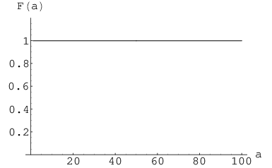
From Eq. (3.67) we see that only if the factor ℱ⁡[a]{\cal F}[a] is independent of its argument a≡x−za\equiv x-z the whole expression IH​SSO⁡(2,2)I_{HS}^{\mathrm{SO}(2,2)} can be in the desired Gaussian form. It needs only a few lines of Maple or Mathematica code to check numerically that actually ℱ⁡[a]≡1{\cal F}[a]\equiv 1, see Fig.1.

Refer to caption
Figure 1: Function F⁡(a)=1F(a)=1 is a constant which does not depend on aa.

Unfortunately, we were not able to find a way of verifying this miraculous identity analytically, as we managed to do in the previous case of O(2,1)(2,1) integral. Nevertheless, we do not think the numerical data leave any doubt in the validity of our claim.

In conclusion, the above calculation shows that for A^=T^0​diag​(x,x,z,z)​T^0−1\hat{A}=\hat{T}_{0}\ \!\textrm{diag}(x,x,z,z)\ \!\hat{T}^{-1}_{0} and T^0∈O⁡(2,2)\hat{T}_{0}\in\mathrm{O}(2,2),

∫𝒟​R^​e−12​Tr​R^2−i​Tr​R^​A^=const​e−12​Tr​A^2,\displaystyle\int\mathcal{D}\hat{R}\ e^{-\frac{1}{2}\mathrm{Tr}\hat{R}^{2}-i\mathrm{Tr}\hat{R}\hat{A}}=\mathrm{const}\,\ e^{-\frac{1}{2}\mathrm{Tr}\hat{A}^{2}}, (3.71)

provided measure for P^\hat{P} integral is chosen to be Eq. (3.66).

It is again interesting to check what will be the result if we choose d​P^=|Δ⁡(P^)|​∏i=14d​pid\hat{P}=|\Delta(\hat{P})|\prod_{i=1}^{4}dp_{i} instead of Eq. (3.66). It is shown in App. E that this choice will make the Hubbard-Stratonovich identity invalid.

Acknowledgements

The research was supported by EPSRC grant EP/C515056/1”Random Matrices and Polynomials: a tool to understand complexity”. The authors are grateful to M.R. Zirnbauer for discussions and hospitality extended to them at the initial stage of the present research which took place at the Institute of Theoretical Physics, University of Cologne, Germany.

Appendix A Proof of Eq. (2.42)

Introducing the set of new variables

a=12​(p1−p2),b=12​(p1+p2),c=p3\displaystyle a=\frac{1}{2}(p_{1}-p_{2}),\quad b=\frac{1}{2}(p_{1}+p_{2}),\quad c=p_{3} (A.72)

and defining t=r21−r2t=\frac{r^{2}}{1-r^{2}}, we can rewrite Eq. (2.41) as

IH​SO⁡(2,1)=∫0∞d​t1+t\displaystyle I_{HS}^{\mathrm{O}(2,1)}=\int_{0}^{\infty}\!\!\frac{dt}{\sqrt{1+t}} ∫0∞da∫−∞∞dbdca[(b−c)2−a2]exp{−a2−b2−c22+i[x(b+c)+zb]\displaystyle\int_{0}^{\infty}\!\!da\int_{-\infty}^{\infty}dbdc\ a[(b-c)^{2}-a^{2}]\exp\bigg\{-a^{2}-b^{2}-\frac{c^{2}}{2}+i[x(b+c)+zb]
+icos2θta(x−z)+i(1+t)(x−z)(b−c)}J0(A2+B2),\displaystyle+i\cos 2\theta\ ta(x-z)+i(1+t)(x-z)(b-c)\bigg\}J_{0}(\sqrt{A^{2}+B^{2}})\,, (A.73)

where we have used Eq. (2.18). Next, we verify that

A2+B2\displaystyle A^{2}+B^{2} =w2​{t2​(b−c)2+2​t​(t+2)​cos⁡2​θ​a​(b−c)+a2​[t2​cos2⁡2​θ+4​(t+1)]}\displaystyle=w^{2}\bigg\{t^{2}(b-c)^{2}+2t(t+2)\cos 2\theta\ a(b-c)+a^{2}[t^{2}\cos^{2}2\theta+4(t+1)]\bigg\}
=w2​{[t⁡(b−c)+a⁡(t+2)​cos⁡2​θ]2+a2​[4​(t+1)​sin2⁡2​θ]}\displaystyle=w^{2}\bigg\{[t(b-c)+a(t+2)\cos 2\theta]^{2}+a^{2}[4(t+1)\sin^{2}2\theta]\bigg\}
=C2+D2,\displaystyle=C^{2}+D^{2}\,, (A.74)

where we defined

C=\displaystyle C= w⁡[t⁡(b−c)+a⁡(t+2)​cos⁡2​θ]\displaystyle w[t(b-c)+a(t+2)\cos 2\theta]
D=\displaystyle D= 2​w​a​t+1​sin⁡2​θ.\displaystyle 2wa\sqrt{t+1}\sin 2\theta\,. (A.75)

This allows us to write (cf. (2.39))

J0​(A2+B2)=1π​∫0πd​ϕ​exp⁡(i​cos⁡ϕ​C+i​sin⁡ϕ​D).\displaystyle J_{0}(\sqrt{A^{2}+B^{2}})=\frac{1}{\pi}\int_{0}^{\pi}d\phi\exp\big(i\cos\phi C+i\sin\phi D\big)\,. (A.76)

Using this representation of the Bessel function in Eq. (A) and defining y=1/1+ty=1/\sqrt{1+t}, we can readily carry out integrals over aa, bb, cc and θ\theta, and get

IH​SO⁡(2,1)=exp⁡[−x2−z22]​F​(w),\displaystyle I_{HS}^{\mathrm{O}(2,1)}=\exp[-x^{2}-\frac{z^{2}}{2}]F(w)\,, (A.77)

where we defined

F⁡(w)=∫1∞d​y​∫0πd​ϕ​exp⁡{−[w2−(x−z)2]​y2−[w​cos⁡ϕ⁡(y2−1)+(x−z)​y2]2}.\displaystyle F(w)=\int_{1}^{\infty}dy\int_{0}^{\pi}d\phi\exp\bigg\{-[w^{2}-(x-z)^{2}]y^{2}-[w\cos\phi(y^{2}-1)+(x-z)y^{2}]^{2}\bigg\}\,. (A.78)

Note that although the above integral formally seems to depend on both ww and (x−z)(x-z), we shall see below that it is a function of ww only and is actually independent of the second combination.

To calculate F⁡(w)F(w) we find it convenient to apply first the standard Hubbard-Stratonovich transformation and ”linearise” the second term in the exponent by introducing an auxiliary Gaussian integral:

F(w)=∫1∞dy∫0πdϕ∫−∞∞dhexp{\displaystyle F(w)=\int_{1}^{\infty}dy\int_{0}^{\pi}d\phi\int_{-\infty}^{\infty}dh\exp\bigg\{ −[w2−(x−z)2]​y2−h2\displaystyle-[w^{2}-(x-z)^{2}]y^{2}-h^{2}
+2ih[wcosϕ(y2−1)+(x−z)y2]}.\displaystyle+2ih\ [w\cos\phi(y^{2}-1)+(x-z)y^{2}]\bigg\}\,. (A.79)

Integration over ϕ\phi yields the Bessel function which can be expanded in its Taylor series, and the Gaussian integral over hh can be performed. In this way we find

F⁡(w)=const​∑n=0∞w2​n​∫1∞d​y​e−(x−z)2​(y4−y2)​{[1y2−2​(1−2​y2)​(x−z)2]​Cn+2​(1−2​y2)​Cn−1}\displaystyle F(w)={\mathrm{const}}\sum_{n=0}^{\infty}w^{2n}\!\int_{1}^{\infty}\!\!dy\ e^{-(x-z)^{2}(y^{4}-y^{2})}\bigg\{\left[\frac{1}{y^{2}}-2(1-2y^{2})(x-z)^{2}\right]C_{n}+2(1-2y^{2})C_{n-1}\bigg\} (A.80)

where we defined for n≥0n\geq 0

Cn=∑m=0n(−)n−m(n−m)!​y2​(n−m)​(y2−1)2​m​(2​m)!m!​m!​∑k=0m(−)k4k​k!​[(x−z)​y2]2​m−2​k(2​m−2​k)!\displaystyle C_{n}=\sum_{m=0}^{n}\frac{(-)^{n-m}}{(n-m)!}y^{2(n-m)}(y^{2}-1)^{2m}\frac{(2m)!}{m!m!}\sum_{k=0}^{m}\frac{(-)^{k}}{4^{k}k!}\frac{[(x-z)y^{2}]^{2m-2k}}{(2m-2k)!} (A.81)

and Cn=0C_{n}=0 for n<0n<0. In particular, the definition above implies

Cn|y=1=(−)nn!.\displaystyle C_{n}\bigg\lvert_{y=1}=\frac{(-)^{n}}{n!}\,. (A.82)

F⁡(w)F(w) can be found as we are now able to perform the integrations on the right-hand side of Eq. (A.80) as

∫1∞d​y​e−(x−z)2​(y4−y2)​{[1y2−2​(1−2​y2)​(x−z)2]​Cn+2​(1−2​y2)​Cn−1}\displaystyle\int_{1}^{\infty}\!\!dy\ e^{-(x-z)^{2}(y^{4}-y^{2})}\bigg\{[\frac{1}{y^{2}}-2(1-2y^{2})(x-z)^{2}]C_{n}+2(1-2y^{2})C_{n-1}\bigg\}
=\displaystyle= −e−(x−z)2​(y4−y2)y[Cn+y2(y2−1)∑i=0n−1an,iCi]|y=1∞\displaystyle-\frac{e^{-(x-z)^{2}(y^{4}-y^{2})}}{y}\big[C_{n}+y^{2}(y^{2}-1)\sum_{i=0}^{n-1}a_{n,i}C_{i}\big]\bigg\lvert_{y=1}^{\infty}
=\displaystyle= (−)nn!.\displaystyle\frac{(-)^{n}}{n!}\,. (A.83)

Here an,ia_{n,i}’s are coefficients satisfying the following recursive relations

an,n−1=2n,andan.i=−1n​an−1,i,i=0,…,n−2,a1,0=2.\displaystyle a_{n,n-1}=\frac{2}{n},\ \ \ \mathrm{and}\ \ \ a_{n.i}=-\frac{1}{n}a_{n-1,i},\ \ \ \ i=0,\dots,n-2,\ \ \ a_{1,0}=2. (A.84)

In the last step of Eq. (A) we used the fact x−z>0x-z>0. We finally see that Eq. (A) implies the desired Gaussian expression

F⁡(w)=const​e−w2\displaystyle F(w)={\mathrm{const}}\,e^{-w^{2}} (A.85)

Finally, substituting F⁡(w)∝e−w2F(w)\propto e^{-w^{2}} back to Eq. (A.77) completes our proof of Eq. (2.42).

Appendix B Calculation with the naive choice of the volume element D​P^D\hat{P} for O(2,1)(2,1) case

In this appendix, we show the Hubbard-Stratonovich transformation for the O(2,1)(2,1) Pruisken-Schäfer domain is invalid if the volume element is chosen to be D​P^=|Δ⁡(P^)|​∏i=13d​piD\hat{P}=|\Delta(\hat{P})|\prod_{i=1}^{3}dp_{i}.

Starting from Eq. (2.32), we make a change of integration variables as in Eq. (A.72). Then we write Eq. (2.32) as

ℐH​SO⁡(2,1)=∫0∞d​t1+t​∫−∞∞𝒟​P^​e−a2−b2−c22+i⁡(2​x​b+z​c)+i​t​(x−z)​(b−c)​J0​[t⁡(x−z)​a],\displaystyle\mathcal{I}_{HS}^{\mathrm{O}(2,1)}=\int_{0}^{\infty}\frac{dt}{\sqrt{1+t}}\int_{-\infty}^{\infty}\mathcal{D}\hat{P}\ e^{-a^{2}-b^{2}-\frac{c^{2}}{2}+i(2xb+zc)+it(x-z)(b-c)}J_{0}\left[t(x-z)a\right]\,, (B.86)

where

D​P^=2​|a⁡((b−c)2−a2)|​d​a​d​b​d​c.\displaystyle D\hat{P}=2|a((b-c)^{2}-a^{2})|\ \!da\ \!db\ \!dc\,. (B.87)

We rewrite the above integral as

ℐH​SO⁡(2,1)=ℐH​S,1O⁡(2,1)+ℐH​S,2O⁡(2,1),\displaystyle\mathcal{I}_{HS}^{\mathrm{O}(2,1)}=\mathcal{I}_{HS,1}^{\mathrm{O}(2,1)}+\mathcal{I}_{HS,2}^{\mathrm{O}(2,1)}\,, (B.88)

where we defined

ℐH​S,1O⁡(2,1)=∫0∞d​t1+t∫−∞∞\displaystyle\mathcal{I}_{HS,1}^{\mathrm{O}(2,1)}=\int_{0}^{\infty}\frac{dt}{\sqrt{1+t}}\int_{-\infty}^{\infty} 2​|a|​((b−c)2−a2)​d​a​d​b​d​c​e−a2−b2−c22+i⁡(2​x​b+z​c)+i​t​(x−z)​(b−c)\displaystyle 2|a|((b-c)^{2}-a^{2})\ \!da\ \!db\ \!dc\ e^{-a^{2}-b^{2}-\frac{c^{2}}{2}+i(2xb+zc)+it(x-z)(b-c)}
J0​[t​(x−z)​a]\displaystyle J_{0}\left[t(x-z)a\right] (B.89)

and

ℐH​S,2O⁡(2,1)=∫0∞d​t1+t∫0|b−c|\displaystyle\mathcal{I}_{HS,2}^{\mathrm{O}(2,1)}=\int_{0}^{\infty}\!\!\frac{dt}{\sqrt{1+t}}\int_{0}^{|b-c|} 4​|a|​(a2−(b−c)2)​𝑑a​∫−∞∞d​b​𝑑c​e−a2−b2−c22+i⁡(2​x​b+z​c)+i​t​(x−z)​(b−c)\displaystyle\!\!\!4|a|(a^{2}-(b-c)^{2})\ \!da\int_{-\infty}^{\infty}\!\!dbdc\ e^{-a^{2}-b^{2}-\frac{c^{2}}{2}+i(2xb+zc)+it(x-z)(b-c)}
J0​[t​(x−z)​a].\displaystyle J_{0}\left[t(x-z)a\right]. (B.90)

Let us stress that it is the contribution ℐH​S,2O⁡(2,1)\mathcal{I}_{HS,2}^{\mathrm{O}(2,1)} which encapsulates the difference between the definition D​P^=|Δ⁡(P^)|​∏i=13d​piD\hat{P}=|\Delta(\hat{P})|\prod_{i=1}^{3}dp_{i} which is positive definite and Eq. (2.18) which is sign indefinite. Such a term has cancelled out when we the volume element was chosen to be Eq. (2.18). The first contribution ℐH​S,1O⁡(2,1)\mathcal{I}_{HS,1}^{\mathrm{O}(2,1)} is nothing else but the IH​SO⁡(2,1)I_{HS}^{\mathrm{O}(2,1)} calculated in the Section 2, and we proved it is in the Gaussian form

ℐH​SO⁡(2,1)=c​o​n​s​t.exp⁡[−12​(2​x2+z2)]+ℐH​S,2O⁡(2,1).\displaystyle\mathcal{I}_{HS}^{\mathrm{O}(2,1)}=const.\exp\bigg[-\frac{1}{2}(2x^{2}+z^{2})\bigg]+\mathcal{I}_{HS,2}^{\mathrm{O}(2,1)}\ \!. (B.91)

In the remaining part of this appendix we will demonstrate that the first contribution ℐH​S,2O⁡(2,1)\mathcal{I}_{HS,2}^{\mathrm{O}(2,1)} is not in a Gaussian form, thus invalidating the Hubbard-Stratonovich transformation.

Define m=b+cm=b+c, n=b−cn=b-c and integrate over mm. We get

ℐH​S,2O⁡(2,1)=\displaystyle\mathcal{I}_{HS,2}^{\mathrm{O}(2,1)}= 2​6​π3​exp⁡[−16​(2​x+z)2]​∫−∞∞d​n​n4​exp⁡{−(13+a2)​n2+i​n​(x−z)​(23+t)}\displaystyle\frac{2\sqrt{6\pi}}{3}\exp\big[-\frac{1}{6}(2x+z)^{2}\big]\int_{-\infty}^{\infty}dn\ n^{4}\exp\bigg\{-(\frac{1}{3}+a^{2})n^{2}+in(x-z)(\frac{2}{3}+t)\bigg\}
∫01d​a​∫0∞d​t1+t​a​(a2−1)​J0​[t⁡(x−z)​n​a].\displaystyle\int_{0}^{1}da\int_{0}^{\infty}\frac{dt}{\sqrt{1+t}}a(a^{2}-1)J_{0}\bigg[t(x-z)na\bigg]\ \!. (B.92)

It is clear that ℐH​S,2O⁡(2,1)\mathcal{I}_{HS,2}^{\mathrm{O}(2,1)} will be in the desired Gaussian form if integral part of the above formula is ∝exp(−(x−z)2/3)\propto\exp(-(x-z)^{2}/3). To check this, it is sufficient to consider a special case x→zx\to z, i.e. |x−z|≪1|x-z|\ll 1. In this limit, we can approximate the integral by setting the argument of the Bessel function in the integrand to zero. This gives

ℐH​S,2O⁡(2,1)∝e−(2​x+z)26\displaystyle\mathcal{I}_{HS,2}^{\mathrm{O}(2,1)}\propto e^{-\frac{(2x+z)^{2}}{6}} ∫0∞d​t1+t​∫−∞∞d​n​n4​exp⁡{−13​n2+i​n​(x−z)​(23+t)}\displaystyle\int_{0}^{\infty}\frac{dt}{\sqrt{1+t}}\int_{-\infty}^{\infty}dn\ n^{4}\exp\bigg\{-\frac{1}{3}n^{2}+in(x-z)(\frac{2}{3}+t)\bigg\}
∫01d​a​a​(a2−1)​exp⁡(−n2​a2).\displaystyle\int_{0}^{1}daa(a^{2}-1)\exp(-n^{2}a^{2})\,. (B.93)

The integral over aa is simply

∫01d​a​a​(1−a2)​exp⁡(−n2​a2)=12​n4​[exp⁡(−n2)+n2−1].\displaystyle\int_{0}^{1}da\ \!a(1-a^{2})\exp(-n^{2}a^{2})=\frac{1}{2n^{4}}[\exp(-n^{2})+n^{2}-1]. (B.94)

Carrying out the standard Gaussian integrals over nn, we get

ℐH​S,2O⁡(2,1)∝e−(2​x+z)26∫0∞d​t1+t[12[(x−z)2(3t+2)2−2]\displaystyle\mathcal{I}_{HS,2}^{\mathrm{O}(2,1)}\propto e^{-\frac{(2x+z)^{2}}{6}}\int_{0}^{\infty}\frac{dt}{\sqrt{1+t}}\bigg[\frac{1}{2}\big[(x-z)^{2}(3t+2)^{2}-2\big] e−112​(x−z)2​(3​t+2)2\displaystyle e^{-\frac{1}{12}(x-z)^{2}(3t+2)^{2}}
−e−148​(x−z)2​(3​t+2)2].\displaystyle-e^{-\frac{1}{48}(x-z)^{2}(3t+2)^{2}}\bigg]\,. (B.95)

The integral over tt is divergent if x−z=0x-z=0, as expected, and in the limit |x−z|≪1|x-z|\ll 1 it is a well-defined expression dominated by t∼(x−z)−1≫1t\sim(x-z)^{-1}\gg 1 so that ℐH​S,2O⁡(2,1)∼(x−z)−1/2\mathcal{I}_{HS,2}^{\mathrm{O}(2,1)}\sim(x-z)^{-1/2}. Such a pre-exponential factor clearly precludes the expression to be in the desired Gaussian form.

Appendix C Calculations for the standard case O(3)(3)

In this appendix, we repeat calculations similar to those in section 2 and App. B, but this time for the compact case of O(3)(3) group. Although the Hubbard-Stratonovich transformation for O(3)(3) symmetry is trivially valid in the original formulation, it is instructive to have a comparison between O(3)(3) and O(2,1)(2,1) in the polar representation, as it helps to understand peculiarities of the non-compact case.

First, we consider an integral similar to Eq. (2.17), with integration of T^\hat{T} going this time over O⁡(3)\mathrm{O}(3) instead of O(2,1)(2,1). We consider only the simplest case setting A^=diag​(x,x,z)\hat{A}=\textrm{diag}(x,x,z) and deal with the following integral

IH​SO⁡(3)=∫𝒟R^e−12​Tr​R^2−i​Tr​R^​A^=∫−∞∞𝒟P^e−12∑i=13pi2∫G/Hdμ(S^)e−i​Tr​S^−1​P^​S^​A^,\displaystyle I_{HS}^{\mathrm{O}(3)}=\int\mathcal{D}\hat{R}\ e^{-\frac{1}{2}\mathrm{Tr}\hat{R}^{2}-i\mathrm{Tr}\hat{R}\hat{A}}=\int_{-\infty}^{\infty}\mathcal{D}\hat{P}e^{-\frac{1}{2}\sum\limits_{i=1}^{3}p_{i}^{2}}\int_{G/H}d\mu(\hat{S})\ e^{-i\mathrm{Tr}\hat{S}^{-1}\hat{P}\hat{S}\hat{A}}\,, (C.96)

where G=O⁡(3)G=\mathrm{O}(3) and H=O⁡(2)×O⁡(1)H=\mathrm{O}(2)\times\mathrm{O}(1). Elements of this compact coset is parametrised as

s=gH=((1+Z​ZT)−12Z​(1+ZT​Z)−12ZT​(1+Z​ZT)−12(1+ZT​Z)−12),\displaystyle s=g_{H}=\left(\begin{array}[]{cc}(1+ZZ^{T})^{-\frac{1}{2}}&Z(1+Z^{T}Z)^{-\frac{1}{2}}\\ Z^{T}(1+ZZ^{T})^{-\frac{1}{2}}&(1+Z^{T}Z)^{-\frac{1}{2}}\end{array}\right),

where we introduced the 2×12\times 1 real matrix ZZ as the convenient coordinate on G/HG/H, with

Z=(z1z2),withz1​and​z2​arbitrary​real.\displaystyle Z=\left(\begin{array}[]{c}z_{1}\\ z_{2}\end{array}\right)\,,\quad\mbox{with}\quad\ {\mathrm{z_{1}\ and\ z_{2}\ arbitrary\ real.}}

Similar to the non-compact case, s−1​(Z,ZT)=s⁡(−Z,−ZT)s^{-1}(Z,Z^{T})=s(-Z,-Z^{T}). The invariant measure d​μ​(S^)d\mu(\hat{S}) in the projective coordinates is given by

d​μ​(S^)=d​Z​d​ZT(1+ZT​Z)32,whered​Z​d​ZT=d​z1​d​z2.\displaystyle d\mu(\hat{S})=\frac{dZdZ^{T}}{(1+Z^{T}Z)^{\frac{3}{2}}}\,,\quad\mbox{where}\quad dZdZ^{T}=dz_{1}dz_{2}\,. (C.101)

The integration over the coset is now straightforward and calculations are done parallel to those in section 2. After some algebra and a few changes of variables, we get

IH​SO⁡(3)=∫01d​t1−t​∫−∞∞𝒟​P^\displaystyle I_{HS}^{\mathrm{O}(3)}=\int_{0}^{1}\frac{dt}{\sqrt{1-t}}\int_{-\infty}^{\infty}\mathcal{D}\hat{P}\ exp{−12∑i=13pi2+i(x(p1+p2)+zp3)\displaystyle\exp\bigg\{-\frac{1}{2}\sum\limits_{i=1}^{3}p_{i}^{2}+i(x(p_{1}+p_{2})+zp_{3})
+i​t2(z−x)(p1+p2−2p3)}J0[t2(x−z)(p1−p2)].\displaystyle+\frac{it}{2}(z-x)(p_{1}+p_{2}-2p_{3})\bigg\}J_{0}\left[\frac{t}{2}(x-z)(p_{1}-p_{2})\right]\,. (C.102)

The difference between Eq. (C.102) and Eq. (2.32) is due to the difference between compact and non-compact integration manifolds.

A crucial difference in the O(3)(3) case is that the volume elements 𝒟​P^\mathcal{D}\hat{P} in the above formula is 𝒟​P^=|Δ⁡(P^)|​∏i=13d​pi\mathcal{D}\hat{P}=|\Delta(\hat{P})|\prod_{i=1}^{3}dp_{i}, instead of Eq. (2.18). We have seen in App. B that this choice of 𝒟​P^\mathcal{D}\hat{P} when applied for O(2,1)(2,1) symmetry would yield a form which is not Gaussian. In the remaining part of this appendix we show that in the case of O(3)(3) the result is in contrast Gaussian.

Define the same set of integration variables as Eq. (A.72) and use them in Eq. (C.102). We have

ℐH​SO⁡(3)=ℐH​S,1O⁡(3)+ℐH​S,2O⁡(3),\displaystyle\mathcal{I}_{HS}^{\mathrm{O}(3)}=\mathcal{I}_{HS,1}^{\mathrm{O}(3)}+\mathcal{I}_{HS,2}^{\mathrm{O}(3)}\,, (C.103)

where we defined

ℐH​S,1O⁡(3)=∫01d​t1−t∫−∞∞\displaystyle\mathcal{I}_{HS,1}^{\mathrm{O}(3)}=\int_{0}^{1}\frac{dt}{\sqrt{1-t}}\int_{-\infty}^{\infty} 2​|a|​((b−c)2−a2)​d​a​d​b​d​c​e−a2−b2−c22+i⁡(2​x​a+z​c)−i​t​(x−z)​(a−c)\displaystyle 2|a|((b-c)^{2}-a^{2})\ \!da\ \!db\ \!dc\ e^{-a^{2}-b^{2}-\frac{c^{2}}{2}+i(2xa+zc)-it(x-z)(a-c)}
J0​[t​(x−z)​a]\displaystyle J_{0}\left[t(x-z)a\right] (C.104)

and

ℐH​S,2O⁡(3)=∫01d​t1−t∫0|b−c|\displaystyle\mathcal{I}_{HS,2}^{\mathrm{O}(3)}=\int_{0}^{1}\!\!\frac{dt}{\sqrt{1-t}}\int_{0}^{|b-c|} 4​|a|​(a2−(b−c)2)​𝑑a​∫−∞∞d​b​𝑑c​e−a2−b2−c22+i⁡(2​x​a+z​c)−i​t​(x−z)​(a−c)\displaystyle\!\!\!4|a|(a^{2}-(b-c)^{2})\ \!da\int_{-\infty}^{\infty}\!\!dbdc\ e^{-a^{2}-b^{2}-\frac{c^{2}}{2}+i(2xa+zc)-it(x-z)(a-c)}
J0​[t​(x−z)​a].\displaystyle J_{0}\left[t(x-z)a\right]\ \!. (C.105)

Note again that ℐH​S,1O⁡(3)\mathcal{I}_{HS,1}^{\mathrm{O}(3)} corresponds to the definition Eq. (2.18) and ℐH​S,2O⁡(3)\mathcal{I}_{HS,2}^{\mathrm{O}(3)} emerges only because the volume element is positive definite in the current case.

First, we deal with ℐH​S,1O⁡(3)\mathcal{I}_{HS,1}^{\mathrm{O}(3)}. Carrying out simple Gaussian integrations over aa, bb and cc we find

ℐH​S,1O⁡(3)=2​π32​ℱ1​(x,z)​e−12​(2​x2+z2),\displaystyle\mathcal{I}_{HS,1}^{\mathrm{O}(3)}=\frac{\sqrt{2}\pi}{32}\mathcal{F}_{1}(x,z)e^{-\frac{1}{2}(2x^{2}+z^{2})}\,, (C.106)

where

ℱ1​(x,z)=∫01d​t1−t​exp⁡(−12​(t2+t)​(x−z)2)​[1−(x−z)2​(2​t2+3​t+1)].\displaystyle\mathcal{F}_{1}(x,z)=\int_{0}^{1}\frac{dt}{\sqrt{1-t}}\exp\left(-\frac{1}{2}(t^{2}+t)(x-z)^{2}\right)\left[1-(x-z)^{2}(2t^{2}+3t+1)\right]\,. (C.107)

Using a=(x−z)2a=(x-z)^{2} and y=1−ty=\sqrt{1-t} we immediately see that

ℱ1​(a)\displaystyle\mathcal{F}_{1}(a) =∫01d​t1−t​exp⁡(−12​(t2+t)​(x−z)2)​[1−(x−z)2​(2​t2−3​t+1)]\displaystyle=\int_{0}^{1}\frac{dt}{\sqrt{1-t}}\exp\left(-\frac{1}{2}(t^{2}+t)(x-z)^{2}\right)\left[1-(x-z)^{2}(2t^{2}-3t+1)\right]
=∫01d​y​exp⁡(−a2​(y4−y2))​[1−a⁡(2​y4−y2)]\displaystyle=\int_{0}^{1}dy\ \exp\left(-\frac{a}{2}(y^{4}-y^{2})\right)\left[1-a(2y^{4}-y^{2})\right]
=1−limy→0y​exp⁡(−a​y2​(y2−1)2)=1.\displaystyle=1-\lim_{y\to 0}y\exp(-\frac{ay^{2}(y^{2}-1)}{2})=1\,. (C.108)

Here, the integral over yy is the same as the one in Eq. (2.1) with different upper and lower limits, but the result is the same. This completes our proof that ℐH​S,1O⁡(3)\mathcal{I}_{HS,1}^{\mathrm{O}(3)} indeed in the Gaussian form. We also note there is certain kind of duality between ℐH​S,1O⁡(3)\mathcal{I}_{HS,1}^{\mathrm{O}(3)} and ℐH​SO⁡(2,1)\mathcal{I}_{HS}^{\mathrm{O}(2,1)}.

As we know already, the integral ℐH​SO⁡(3)\mathcal{I}_{HS}^{\mathrm{O}(3)} is of the Gaussian form ∝exp⁡[−x2−z2/2]\propto\exp[-x^{2}-z^{2}/2], and we have just shown that the same holds for ℐH​S,1O⁡(3)\mathcal{I}_{HS,1}^{\mathrm{O}(3)}, the second terms ℐH​S,2O⁡(3)\mathcal{I}_{HS,2}^{\mathrm{O}(3)} can then only be either 0 or the same Gaussian form as ℐH​S,1O⁡(3)\mathcal{I}_{HS,1}^{\mathrm{O}(3)}. To see which is the case, it is sufficient to consider the same limit x→zx\to z as we did in App. B. In the limit |x−z|≪1|x-z|\ll 1, we find

ℐH​S,2O⁡(3)=∫01d​t1−t∫0|b−c|\displaystyle\mathcal{I}_{HS,2}^{\mathrm{O}(3)}=\int_{0}^{1}\!\!\frac{dt}{\sqrt{1-t}}\int_{0}^{|b-c|} 4​|a|​(a2−(b−c)2)​𝑑a​∫−∞∞d​b​𝑑c​e−a2−b2−c22+i⁡(2​x​a+z​c).\displaystyle\!\!\!4|a|(a^{2}-(b-c)^{2})\ \!da\int_{-\infty}^{\infty}\!\!dbdc\ e^{-a^{2}-b^{2}-\frac{c^{2}}{2}+i(2xa+zc)}\,. (C.109)

One can perform all the integrations in this formula explicitly, and show that

ℐH​S,2O⁡(3)∝exp⁡{−12​(2​x2+z2)}\displaystyle\mathcal{I}_{HS,2}^{\mathrm{O}(3)}\propto\exp\big\{-\frac{1}{2}(2x^{2}+z^{2})\big\} (C.110)

as expected.

Appendix D Jacobian of the transformation from ZZ to polar coordinates

Write the polar coordinates decomposition in Eq. (3) as Z=O1​Λ​O2Z=O_{1}\Lambda O_{2}, where Λ=(r00s)\Lambda=\left(\begin{array}[]{cc}r&0\\ 0&s\end{array}\right). We have

{d​Z=d​O1​Λ​O2+O1​d​Λ​O2+O1​Λ​d​O2d​ZT=d​O2T​Λ​O1+O2T​d​Λ​O1+O2T​Λ​d​O1.\displaystyle\left\{\begin{array}[]{l}dZ\ \ =dO_{1}\Lambda O_{2}+O_{1}d\Lambda O_{2}+O_{1}\Lambda dO_{2}\\ dZ^{T}=dO_{2}^{T}\Lambda O_{1}+O_{2}^{T}d\Lambda O_{1}+O_{2}^{T}\Lambda dO_{1}\end{array}\ \!.\right.

Following the standard way of derivation, see e.g.[21], we have

d2​S=Tr​d​Z​d​ZT=Tr\displaystyle d^{2}S=\mathrm{Tr}\ dZdZ^{T}=\mathrm{Tr}\ {O1TdO1ΛO2dO2TΛ+ΛdΛO2dO2T+Λ2dO2dO2T\displaystyle\bigg\{O_{1}^{T}dO_{1}\Lambda O_{2}dO_{2}^{T}\Lambda+\Lambda d\Lambda O_{2}dO_{2}^{T}+\Lambda^{2}dO_{2}dO_{2}^{T}
+O1T​d​O1​Λ​d​Λ+d2​Λ+Λ​d​Λ​d​O2​O2T\displaystyle+O_{1}^{T}dO_{1}\Lambda d\Lambda+d^{2}\Lambda+\Lambda d\Lambda dO_{2}O_{2}^{T}
+Λ2dO1TdO1+ΛdΛdO1TO1+ΛdO2O2TΛdO1TO1}.\displaystyle+\Lambda^{2}dO_{1}^{T}dO_{1}+\Lambda d\Lambda dO_{1}^{T}O_{1}+\Lambda dO_{2}O_{2}^{T}\Lambda dO_{1}^{T}O_{1}\bigg\}. (D.113)

Next we define

{δ​O1=O1T​d​O1δ​O2=d​O2​O2T.\displaystyle\left\{\begin{array}[]{l}\delta O_{1}=O_{1}^{T}dO_{1}\\ \delta O_{2}=dO_{2}O_{2}^{T}\end{array}\right.\,.

Recalling that δ​O1\delta O_{1} and δ​O2\delta O_{2} are skew-symmetric matrices, which can be written as

δ​O1=(0δ​O1,12−δ​O1,120),δ​O2=(0δ​O2,12−δ​O2,120).\displaystyle\delta O_{1}=\left(\begin{array}[]{cc}0&\delta O_{1,12}\\ -\delta O_{1,12}&0\end{array}\right),\hskip 14.22636pt\delta O_{2}=\left(\begin{array}[]{cc}0&\delta O_{2,12}\\ -\delta O_{2,12}&0\end{array}\right)\,.

We find

d2​S\displaystyle d^{2}S =Tr⁡{d2​Λ−Λ2​δ​O1​δ​O1−Λ2​δ​O2​δ​O2−2​Λ​δ​O1​Λ​δ​O2}\displaystyle=\mathrm{Tr}\bigg\{d^{2}\Lambda-\Lambda^{2}\delta O_{1}\delta O_{1}-\Lambda^{2}\delta O_{2}\delta O_{2}-2\Lambda\delta O_{1}\Lambda\delta O_{2}\bigg\}
=(δ​O1,12,δ​O2,12,d​r,d​s)​(r2+s22​r​s2​r​sr2+s211)​(δ​O1,12δ​O2,12d​rd​s)\displaystyle=(\delta O_{1,12},\delta O_{2,12},dr,ds)\left(\begin{array}[]{cccc}r^{2}+s^{2}&2rs&&\\ 2rs&r^{2}+s^{2}&&\\ &&1&\\ &&&1\end{array}\right)\left(\begin{array}[]{c}\delta O_{1,12}\\ \delta O_{2,12}\\ dr\\ ds\end{array}\right)
=d​xi​gi​j​d​xj.\displaystyle=dx^{i}g_{ij}dx^{j}\,. (D.128)

In the last step the summation over repeated indices is assumed. Jacobian is then given by

Jacobian=detg=|r2−s2|.\displaystyle\mathrm{Jacobian}=\sqrt{\det g}=|r^{2}-s^{2}|\ \!. (D.129)

Appendix E Calculation with the alternative volume element D​P^D\hat{P} for O(2,2)(2,2) case

In this appendix, we calculate Eq. (3.47) with the volume element D​P^=|Δ⁡[P^]|​∏i=14d​piD\hat{P}=|\Delta[\hat{P}]|\prod_{i=1}^{4}dp_{i} used instead of Eq. (3.66). We show that by this choice the final result is not in the Gaussian form, hence the corresponding Hubbard-Stratonovich transformation can not be valid.

First we redefine the integration variables

{a=12​(p1+p2)b=12​(p1−p2)c=12​(p3+p4)d=12​(p3−p4).\displaystyle\left\{\begin{array}[]{l}a=\frac{1}{2}(p_{1}+p_{2})\\ b=\hskip 1.42262pt\frac{1}{2}(p_{1}-p_{2})\\ c=\hskip 1.42262pt\frac{1}{2}(p_{3}+p_{4})\\ d=\frac{1}{2}(p_{3}-p_{4})\ \!.\end{array}\right.

Then we have

|Δ⁡[P^]|=4​|b​d|⋅|[(a−c+d)2−b2]​[(a−c−d)2−b2]|.\displaystyle|\Delta[\hat{P}]|=4|bd|\!\cdot\!|[(a-c+d)^{2}-b^{2}][(a-c-d)^{2}-b^{2}]|. (E.134)

Use Eq. (3) and the D​P^D\hat{P} defined above to find

ℐH​SO⁡(2,2)=∫1∞\displaystyle\mathcal{I}_{HS}^{\mathrm{O}(2,2)}=\int_{1}^{\infty} |u−v|​d​u​d​vu⁡(u−1)​v⁡(v−1)​∫D​P^​e−a2−b2−c2−d2+i⁡(x−z)​(a−c)​(u+v)\displaystyle\frac{|u-v|dudv}{\sqrt{u(u-1)}\sqrt{v(v-1)}}\int D{\hat{P}}\ e^{-a^{2}-b^{2}-c^{2}-d^{2}+i(x-z)(a-c)(u+v)}
J0​[b⁡(x−z)​(u−v)]​J0​[d⁡(x−z)​(u−v)].\displaystyle J_{0}\left[b(x-z)(u-v)\right]J_{0}\left[d(x-z)(u-v)\right]. (E.135)

As in App. B we can split ℐH​SO⁡(2,2)\mathcal{I}_{HS}^{\mathrm{O}(2,2)} into two parts,

ℐH​SO⁡(2,2)=ℐH​S,1O⁡(2,2)+ℐH​S,2O⁡(2,2).\displaystyle\mathcal{I}_{HS}^{\mathrm{O}(2,2)}=\mathcal{I}_{HS,1}^{\mathrm{O}(2,2)}+\mathcal{I}_{HS,2}^{\mathrm{O}(2,2)}\ \!. (E.136)

Here, the contribution ℐH​S,1O⁡(2,2)\mathcal{I}_{HS,1}^{\mathrm{O}(2,2)} is precisely the IH​SO⁡(2,2)I_{HS}^{\mathrm{O}(2,2)} we calculated in section 3, and we know it is in a Gaussian form. It is the second contribution, ℐH​S,2O⁡(2,2)\mathcal{I}_{HS,2}^{\mathrm{O}(2,2)}, which arises from the difference between the two definitions of D​P^D\hat{P}, and it is given by

ℐH​S,2O⁡(2,2)∝\displaystyle\mathcal{I}_{HS,2}^{\mathrm{O}(2,2)}\propto ∫−∞∞d​a​𝑑c​∫0∞d​d​∫||a−c|−d||a−c|+dd​b​b​d​[(a−c+d)2−b2]​[(a−c−d)2−b2]\displaystyle\int_{-\infty}^{\infty}dadc\int_{0}^{\infty}dd\int_{||a-c|-d|}^{|a-c|+d}db\ bd[(a-c+d)^{2}-b^{2}][(a-c-d)^{2}-b^{2}]
∫1∞|u−v|​d​u​d​vu⁡(u−1)​v⁡(v−1)​e−a2−b2−c2−d2+2​i​x​c+2​i​z​a+i⁡(x−z)​(a−c)​(u+v)\displaystyle\int_{1}^{\infty}\frac{|u-v|dudv}{\sqrt{u(u-1)}\sqrt{v(v-1)}}\ e^{-a^{2}-b^{2}-c^{2}-d^{2}+2ixc+2iza+i(x-z)(a-c)(u+v)}
J0​[b⁡(x−z)​(u−v)]​J0​[d⁡(x−z)​(u−v)].\displaystyle\hskip 22.76219ptJ_{0}\left[b(x-z)(u-v)\right]J_{0}\left[d(x-z)(u-v)\right]\ \!. (E.137)

In the remaining part of this section we demonstrate that ℐH​S,2O⁡(2,2)\mathcal{I}_{HS,2}^{\mathrm{O}(2,2)} is not in the Gaussian form, thus ℐH​SO⁡(2,2)\mathcal{I}_{HS}^{\mathrm{O}(2,2)} is not either. Which means that Hubbard-Stratonovich transformation fails with this different choice of D​P^D\hat{P}.

First, we define m=a+cm=a+c and n=a−cn=a-c. It is clear that the integral over mm is decoupled from other integrations and can be easily performed. Again, it is sufficient to consider the limit |x−z|≪1|x-z|\ll 1. For the same reason as in App. B, we set the two Bessel terms to be 1 in this limit. We then have

ℐH​S,2O⁡(2,2)∝\displaystyle\mathcal{I}_{HS,2}^{\mathrm{O}(2,2)}\propto exp⁡{−12​(x+z)2}​∫0∞d​n​∫0∞d​d​∫|n−d|n+dd​b​b​d​[(n+d)2−b2]​[(n−d)2−b2]\displaystyle\exp\{-\frac{1}{2}(x+z)^{2}\}\int_{0}^{\infty}\!dn\int_{0}^{\infty}\!dd\int_{|n-d|}^{n+d}\!db\ bd[(n+d)^{2}-b^{2}][(n-d)^{2}-b^{2}]
∫1∞|u−v|​d​u​d​vu⁡(u−1)​v⁡(v−1)​exp⁡{−n2−b2−d2}​cos⁡[n⁡(x−z)​(u+v−1)].\displaystyle\int_{1}^{\infty}\!\frac{|u-v|dudv}{\sqrt{u(u-1)}\sqrt{v(v-1)}}\exp\left\{-n^{2}-b^{2}-d^{2}\right\}\cos\left[n(x-z)(u+v-1)\right]\,. (E.138)

The integral part of the above formula needs to be ∝exp⁡{−12​(x−z)2}\propto\exp\{-\frac{1}{2}(x-z)^{2}\} in order to make ℐH​S,2O⁡(2,2)\mathcal{I}_{HS,2}^{\mathrm{O}(2,2)} be Gaussian. The remaining calculations are lengthy but direct. We perform Gaussian type integrals over bb, dd and nn then define new integration variables X=u+v−1X=u+v-1 and Y=u−vY=u-v. After integrating over YY we get

ℐH​S,2O⁡(2,2)∝∫0∞d​X​ln⁡(2​X+1)​{8−2​a2​X2+π​e−a2​X24​a​X​(a2​X2−6)​Erfi​[a​X2]},\displaystyle\mathcal{I}_{HS,2}^{\mathrm{O}(2,2)}\propto\int_{0}^{\infty}dX\ln(2X+1)\big\{8-2a^{2}X^{2}+\sqrt{\pi}e^{-\frac{a^{2}X^{2}}{4}}aX(a^{2}X^{2}-6){\mathrm{Erfi}}[\frac{aX}{2}]\big\}\,, (E.139)

where we defined a=x−za=x-z, and Erfi stands for the error function of imaginary argument. Integrating by parts we bring the above integral to the form

ℐH​S,2O⁡(2,2)∝∫0∞d​X​12​X+1​(a​X4−π8​e−a2​X24​(a2​X2−2)​Erfi​[a​X2]).\displaystyle\mathcal{I}_{HS,2}^{\mathrm{O}(2,2)}\propto\int_{0}^{\infty}dX\ \frac{1}{2X+1}\bigg(\frac{aX}{4}-\frac{\sqrt{\pi}}{8}e^{-\frac{a^{2}X^{2}}{4}}(a^{2}X^{2}-2){\mathrm{Erfi}}[\frac{aX}{2}]\bigg)\,. (E.140)

Again, in the limit |x−z|≪1|x-z|\ll 1 the integral over XX is dominated by the region X∼(x−z)−1≫1X\sim(x-z)^{-1}\gg 1. Changing variable a​X→XaX\to X and expanding in terms of |x−z||x-z|, we find to the lowest order, ℐH​S,2O⁡(2,2)=c0−|x−z|​c1+O⁡((x−z)2)\mathcal{I}_{HS,2}^{\mathrm{O}(2,2)}=c_{0}-|x-z|c_{1}+O((x-z)^{2}), with c0c_{0} and c1c_{1} being some constants. In this way one finds that ℐH​S,2O⁡(2,2)\mathcal{I}_{HS,2}^{\mathrm{O}(2,2)} is a function of (x−z)(x-z), but is clearly not in the Gaussian form. So we conclude that ℐH​SO⁡(2,2)\mathcal{I}_{HS}^{\mathrm{O}(2,2)} is not Gaussian.

References

  • [1] K.B. Efetov, Supersymmetry in Disorder and Chaos, (Cambridge University Press, 1997).
  • [2] A.D. Mirlin, Phys. Rep. 326 (2000) 259.
  • [3] F.Wegner, Zeitsch. Physik 36 (1979) 207.
  • [4] L. Schäfer and F. Wegner, Z. Phys. B 38 (1980) 113.
  • [5] A.M.M. Pruisken and L. Schäfer, Nucl. Phys. B 200 (1982) 20.
  • [6] K.B. Efetov, Adv. Phys. 32 (1983) 53.
  • [7] J.J.M. Verbaarschot, H.A. Weidenmüller, M.R. Zirnbauer, Phys. Rep. 129 (1985) 367.
  • [8] Y.V.Fyodorov and H.-J. Sommers, J. Math. Phys. 38 (1997) 1918.
  • [9] J.J.M. Verbaarschot and T. Wettig, Annu. Rev. Nucl. Part. Sci. 50 (2000) 343.
  • [10] M-L. Mehta Random Matrices, 3rd ed, (Elsevier, 2004)
  • [11] M.R. Zirnbauer, ”The supersymmetry method of random matrix theory”, Encyclopedia of Mathematical Physics, vol. 5, p. 151-160, Eslevier, 2006 [e-preprint arXiv:math-ph/0404057].
  • [12] M.R. Zirnbauer, J. Math. Phys. 37 (1996) 4986.
  • [13] Y.V. Fyodorov, J.Phys: Cond. Mat. 17 (2005) S1915.
  • [14] M.R. Zirnbauer, ”Symmetry classes in random matrix theory”, e-preprint arXiv:math-ph/0404058.
  • [15] Y.V. Fyodorov Nucl. Phys. B 621 (2002) 643.
  • [16] M.R. Zirnbauer, Y. Wei and Y.V. Fyodorov, under preparation.
  • [17] C.Itzykson and J.B. Zuber, J. Math. Phys. 21 (1980) 411; Harish-Chandra, Proc. Nat. Acad. Sci. 42 (1956) 252.
  • [18] Y.V. Fyodorov and E. Strahov, Nucl. Phys. B 630 (2002) 453.
  • [19] T. Guhr and H. Kohler, J. Math. Phys. 43 (2002) 2707.
  • [20] E. Brezin and S. Hikami, Prog. of Theo. Phys. 116 No.3 (2006) 441.
  • [21] L.K. Hua, Harmonic analysis of functions of several complex numbers in the classical domains, (American Mathematical Society, Providence, 1963).
  • [22] I.S. Gradshteyn and I.M. Ryzhik, Table of integrals, series, and products, (Academic Press, 2000).