Generalized Heisenberg Algebras and Fibonacci Series
Abstract
We have constructed a Heisenberg-type algebra generated by the Hamiltonian, the step operators and an auxiliar operator. This algebra describes quantum systems having eigenvalues of the Hamiltonian depending on the eigenvalues of the two previous levels. This happens, for example, for systems having the energy spectrum given by Fibonacci sequence. Moreover, the algebraic structure depends on two functions and . When these two functions are linear we classify, analysing the stability of the fixed points of the functions, the possible representations for this algebra.
| Keywords: Heisenberg algebra; Fibonacci series; quasi-periodic systems; |
| Fock representation. |
| PACS Numbers: 03.65.Fd, 02.10.De |
1 Introduction
Due to their interesting mathematical structure and possible physical applications deformed algebras have attracted much attention in the last twenty years. In 1982 Kulish [1] showed that the underlying algebra of the -Heisenberg spin model was a deformation of the algebra, called nowadays .
Following the technique developed by Schwinger to compose two Heisenberg oscillators to obtain algebra, in 1989 Macfarlane and Biedenharn [2, 3] constructed the algebra using two -oscillators. -oscillator algebra is a deformation of the Heisenberg algebra through a parameter , which reproduces Heisenberg algebra when the parameter .
Since Heisenberg algebra has an important role in several areas of physics it was tempting to search for applications of this new structure. Thus, there was an intense study of possible physical applications of -oscillators and since then some succesfull ones have been described in the literature [4, 5, 6, 7, 8, 9, 10, 11]. They have also been used as a phenomenological approach to study composite particles [12, 13, 14, 15, 16], spectra of atoms and molecules [12, 18, 19, 6, 20, 11], generalized field theory [21, 14, 15, 16] and coherent states [22].
Recently, a new algebraic structure was proposed [24] that generalizes the Heisenberg algebra. This structure contains also -oscillators as a particular case and has been successfully used in some different physical problems [11, 12, 14, 15, 16, 17, 22, 23]. In this new algebra, called Generalized Heisenberg Algebra (GHA), the commutation relations among the operators , and depend on a general analytic functional and are given by:
| (1) |
| (2) |
| (3) |
with and . Identifying the operator with the Hamiltonian of a physical system, this algebra tell us that the eigenvalues ( in Fock space), which are the energy spectrum of the physical system, are obtained by an one-step recurrence (), i.e, each eigenvalue depends on the previous one. Thus, the eigenvalue behavior can be studied by dynamical system techniques, enormously simplifying the task of finding possible representations of the algebra [24].
When the functional is linear we re-obtain the -oscillator algebra [24, 25]; other kinds of functionals give more general algebraic structures than -oscillators [24]. The functional can be, for example, a polynomial and therefore it depends on some parameters (the polynomial coefficients). Depending on the kind of functional and their parameters, finite or infinite representations are allowed [24]. The operator eigenvalues depend on the characteristic function and it can present a variety of different behaviors (monotonously increasing or decreasing, etc, upper limited or not, etc) [24]. For instance, for the functional , where with and being the mass and the length of the well, one obtains the square-well potential algebra [26]. However, there are several systems which cannot be described by such a class of algebras.
Quasi-periodic structures have attracted much interest lately [27]. In particular, Fibonacci sequences were considered in several areas of mathematics and physics [27, 28]. Moreover, it was shown that an electron gas under sudden heating has a quasiequilibrium regime with a quasiperiodic energy distribution [29]. Since most systems having a quasiperiodic energy spectrum cannot be described by the GHA, in this paper we are going to present a first step in this direction. We construct here a Heisenberg-type algebra for a system having the energy spectrum described by a generalized Fibonacci sequence. In order to realize this, we propose a simple algebraic structure depending on two functionals, and . We introduce an operator , being the Hamiltonian of a system 11 1 Instead of calling as it was done in Eqs. (1 - 3), we will call this operator, from now on, directly as ., having eigenvalues obeying the equation , i.e., the eigenvalue of the -th state depends on the two previous eigenvalues. We call this structure a two-step algebra. In order to extend the “one-step algebra” described by the GHA, we introduce also an additional operator .
When both functionals and appearing in the two-step algebra are linear functions, we show that we can re-write both the and operators in Fock space as functions of a single number operator, . The algebraic structure generated by these functionals contains the GHA, -oscillator algebra and is related to other interesting algebras as special cases.
In section II we introduce the two-step generalized Heisenberg algebra. In section III we study the linear case for the algebra, that contains a Fibonacci-like spectra and many other interesting quasi-periodic sequences and we also discuss the types of representations we could find. In section IV we present our conclusions and in the appendix we classify possible representations for the algebra when and , appearing in the algebra, are linear functions.
2 Extended Two-step Heisenberg Algebra
We propose an structure generated by the operators , , and , with and , , being the step operators, the Hamiltonian and , obeying the following relations:
| (4) | |||
| (5) |
| (6) | |||
| (7) |
| (8) | |||
| (9) |
where we have assumed that and are analytical functions. In the Fock space representation of this structure, one has the normalized vacuum state defined by the relations:
| (10) | |||||
| (11) | |||||
| (12) |
where and are real numbers.
A Casimir operator associated with this algebraic relations is
| (13) |
satisfying the following relations:
| (14) |
2.1 Representation Theory
In order to build a representation theory for the structure given by (4-9), let us start with the vacuum state defined by relations (10-12).
The operator acting on the vacuum state produces another vector, say : . It is trivial to see that the new vector is orthogonal to vector . Let us call . The constant can be determined by performing the inner product of and its dual and by using relation (8):
| (15) |
In order to determine the eigenvalue on the state , we have, using equation (4):
| (16) |
In general, it can be proved that:
| (18) | |||||
| (19) | |||||
| (20) | |||||
| (21) |
where
| (22) | |||||
| (23) | |||||
| (24) | |||||
If we combine equations (22) and (23), the two-step dependence of the eigenvalue becomes clear: , where , for all . Choosing different functions and different initial values and , we can construct different Fock space representations for this mathematical structure. In matrix representation, the operators of the algebra can be written as
In the next section, we shall study the case where and are linear functions.
3 The linear case - Generalized Fibonacci Algebra
If we assume and (), the equations (4-9) reduce to
| (42) | |||||
| (43) | |||||
| (44) | |||||
| (45) | |||||
| (46) |
Using Eqs. (22) and (23) for this linear case we get:
| (47) |
| (48) |
The recurrence equation (48) is a difference equation which generates a Generalized Fibonacci Sequence. Hence, the sequence of eigenvalues of the operator follows a Generalized Fibonacci Series. We can write equations (47) and (48) as a two-dimensional linear map, which is more adequate in order to analyze the representation theory of the algebra. This map can be written as:
In [24], the authors have analyzed, for one quantum number, the representation theory of the GHA using dynamical systems techniques . The representations were obtained analyzing the stability of the fixed-points and the cycles of the equation . In this work we have extended the previous effort and analyzed the stability of the fixed-points of the two dimensional system given by Eq. (3).
3.1 Stability Analysis and Representation Theory
The fixed-points of equation (3) can be found by solving the system
The solutions of the previous equation are and for , where . The stability of these fixed points are given by the eigenvalues of the -matrix in Eq. (3.1), which can be calculated by means of the characteristic equation, . These eigenvalues are independent of a specific point in the -space, as the recurrence given by Eq. (3) is linear, and can be written as:
| (63) |
The main possibilities are:
(i) the fixed point is asymptotically stable if
;
an initial point , iterated using Eq. (3),
approaches as the
number of iterations increases;
(ii) if at
least one of the eigenvalues is, in modulus, bigger than one, the fixed point
is called unstable and the iterations of an initial point
by Eq. (3) move this point far away the fixed point.
(iii) if both eigenvalues are, in modulus, equal to one - edge
in Figure (3) -
we call the fixed point
marginally stable . The iterations of an initial
point in the -space will not move it far away the fixed point,
but it will not approach the fixed point too as the iterations increase.
In Figure (3) we show the stability regions of the fixed points and in the parameter space .
When the fixed point is the only fixed point in the space. It is asymptotically stable for values of and inside the triangle and unstable for values of and outside this triangle. It is marginally stable on the edge and, on the edge , where one eigenvalue () is always equal to and the other () is equal to , with , the iteration of any initial point will approach a cycle two, with the line joining them crossing the fixed point in the -space.
If , the dotted line in Figure (3), there are a line of fixed points in the -space, , with . All these fixed points are unstable if, in the line , or , i.e., for points in this line outside the edge (see Figure (3)). For points in this line belonging to the edge , the associated eigenvalues are and , with . The fixed points in the -space, , are stable in one direction, crossing the line of fixed points, associated with the eigenvalue , . The direction along the line of fixed points is marginally stable, associated with the eigenvalue .
In the linear case, given the values of and (or, equivalently, the values of and , see Fig. 5), the possible values of and for the representations of the linear case of the algebra we are analyzing are presented in the appendix. If the two-dimensional map, Eq. (3), has an unstable fixed point (i.e., if the values of and are outside the triangle of Fig. 3), the possible representations are infinite-dimensional and their corresponding spectra have no upper limit; the difference between two consecutive numbers in the corresponding sequence increases as the number of iterations increases. If this map has an asymptotically stable fixed point (i.e., if the values of and are inside the triangle of Fig. 3), the possible representations are also infinite-dimensional but they have superiorly-limited spectra; the difference between two consecutive numbers in the corresponding sequence decreases as the number of iterations increases. The representations associated with marginally stable cases are more complex and, besides infinite-dimensional representations, it is also possible to have finite-dimensional ones. See the appendix for a discussion of the possible values of and for these representations.
3.2 Fibonacci series
If we assume the relation given by equation (48) becomes
| (64) |
which yields the usual Fibonacci sequence if we choose . The Fibonacci series have as eigenvalues . The eigenvalue is the so-called golden-number. The single fixed-point is, therefore, unstable. The representations are infinite dimensional and the sequences (depending on the initial values () ) increase without an upper limit, as we know. Specific values of and describing possible representations for this case will be discussed in the next section. The values of and for are shown in Table 1. The eigenvalues and provide the number of elements of kind “A” and “B”, respectively, in the -th inflation of the Fibonacci chain (Figure 1). Thus, the operator acts as an “inflation operator” of the Fibonacci chain, while the eigenvalues provide the number of elements of the quasiperiodic chain generated at the -th inflation.
4 Fock space two-step Heisenberg algebra
The Generalized Fibonacci Series (Eq. (48)) can be written by means of the so-called Binet formula:
| (65) | |||||
| (66) |
where are the roots given by Eq. (63), and is the two-parameter -number (Gauss Number) [35]. As is the Hamiltonian, the choice of is not completely free inasmuch as we should guarantee that for any (the energy of the ground state must be the lowest one). This condition implies that, once the value of had been chosen, the allowed values of should satisfy the relation
| (67) |
for any value of , . In particular, if for any value of , the condition to be satisfied by can be written as:
| (68) |
for any value of , .
The solution for for the whole parameter space will be described in the appendix. For the specific case of Fibonacci chain () it is simple to see that the term varies from up to . Then, implies and implies that .
We can show that there exist another Casimir Operator when and are linear functions:
| (69) |
where is the deformed number operator and is the usual number operator, defined in Fock space as
| (70) |
Using Eq. (65), it is possible to reduce the algebraic structure (42-46) to a Heisenberg-like structure composed by the usual operators , and . From Eq. (65) can be written in Fock space as:
| (71) |
and, using Eq. (47), can be written as
| (72) |
Note that the effect of the application of and on is exactly the same as if we use Eqs. (71) and (72) on . Substituting and in Eq. (46) by Eqs. (71) and (72) and using Eqs. (20), (21) and (70) we get:
| (73) | |||||
| (74) | |||||
| (75) | |||||
The above algebraic structure is the Fock space form of a two-step Heisenberg algebra. Notice that the algebraic structure described in Eqs. (42-46) correspond to Eqs. (73-75) plus the Hamiltonian , whose eigenvalues follow the generalized Fibonacci sequence.
Remembering that and ( and are roots of ), the right hand side of Eq. (75) can be written as
| (76) |
which, after some algebra allows us to write Eq. (75) as:
| (77) |
Considering and in Eq. (77), Eqs. (73-74) and (77) can be related to the -oscillator, reference [35], which was used in nuclear spectroscopy [36]. Thus, the eigenvalues of the -oscillator can be written as a particular case of the generalized Fibonacci numbers with “initial conditions” and . In our “extended algebra”, the eigenvalues are written as Generalized Fibonacci numbers where the initial values and can assume any value since that for any . Thereby, each set of initial values () define a new representation.
5 Final comments
We have constructed a Heisenberg-type algebra having as generators the Hamiltonian, the step-operators and an auxiliary operator. Moreover, this structure depends on two analytic functions and . Since the energy spectra of the systems described by this algebra depend on the two previous energy levels, this algebra was called generalized two-step Heisenberg algebra.
This algebra describe quantum systems having eigenvalues of the operator (Hamiltonian) analytically depending on the two previous eigenvalues, i. e., , where is a function and is the eigenvalue of acting on the eigenstate , i. e., . A quantum system having the Hamiltonian eigenvalues obeying the Fibonacci sequence (quasi-periodic systems) could, for example, be described by this algebra. Possible spectra generated by this algebra can be seen in Figure 4, showing that the typical possible spectra found in nature can be generated by this algebraic structure.
We have discussed the representations of this algebra and we have classified in detail the possible representations for linear and . To perform this classification we have used tools from dynamical system techniques as the analysis of the stability of the fixed points of the characteristic functions of the algebra, and .
In [12], an algebraic phenomenological approach, based on the GHA, was implemented for the molecule. We think that the algebra constructed here could be used to generalize the mentioned approach to more general spectra.
We also consider mathematically interesting to analyse in detail the representations of this algebra at least for simple nonlinear examples of the characteristic functions.
Appendix
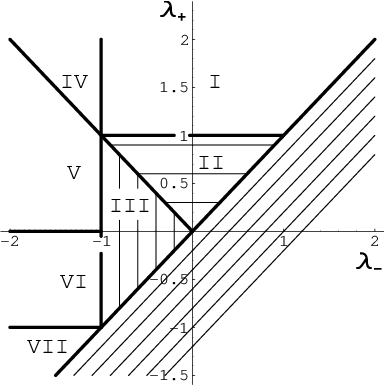
In this appendix we discuss the representations associated with the linear case. In order to classify the possible values of and according to the value of the eigenvalues (or ) and (or ) we divide the plane () in regions labeled by the numbers , , , , and , see figure 5. As, by definition, , only the semi-plane equal and above the diagonal line at in this plane makes sense. The representations of the extended algebra can be obtained providing and satisfy the conditions given by Eqs. (67) and (68). Analysing these equations for the regions labeled from to in Figure 5, it is possible to obtain representations for the extended algebra since and satisfy the following conditions (the results for regions IV, VI and VII are numerical):
Region I: and
a) if
b) if
Region II: and
Region III: and
and
Region IV: and
a) if
b) if
Region V: and
In this region there is no simple general analytical solution for the values
of and and the possible representations should be
computed case by case.
Region VI: and
a) if
b) if
Region VII: , and .
a) if
b) if
The possible expressions for and belonging to the boundaries between these regions are the following:
i) Boundary between region and :
for
ii) Boundary between region and :
The same expressions for and allowed for region
with .
iii) Boundary between region and :
The same expressions for and allowed for region
with .
iv) Boundary between region and :
.
v) Boundary between region and :
The same expressions for and allowed for region
with .
vi) Boundary between region and :
a) If
b) If .
vii) Boundary between region and :
The same expressions for and allowed for region
with .
viii) Boundary between region and :
The same expressions for and allowed for region
with .
References
- [1] Kulish P and Reshetikhin N 1983 J. Sov. Math. 23 2435; Faddeev L D 1982 Les Houches Session XXXIX (Amsterdam: Elsevier)
- [2] Macfarlane A J 1989 J. Phys. A: Math. Gen. 22 L4581
- [3] Biedenharn L C 1989 J. Phys. A: Math. Gen. 22 L873
- [4] Rego-Monteiro M A, Roditi I and Rodrigues L M C S 1994 Phys. Lett.A 188 11
- [5] Angelova M, Dobrev V K, Frank A 2001 J. Phys. A: Math. Gen. 34 L503
- [6] Angelova M N 2002 Phys. Part Nuc. 33: S37 (Suppl. 1)
- [7] Bonatsos D and Daskaloyannis C 1999 Prog. Part. Nucl. Phys. 43 537
- [8] Monteiro M R, Rodrigues L M C S and Wulck S 1996 Phys. Rev. Lett. 76 1098
- [9] Lavagno A and Swamy P N 2002 Phys. Rev. E 65 036101
- [10] Algin A and Deviren B 2005 J. Phys. A: Math. Gen. 38 5945
- [11] Oliveira-Neto N M, Curado E M F, Nobre F D and Rego-Monteiro M A 2004 Physica A 344 573
- [12] de Souza J, Oliveira-Neto N M and Ribeiro-Silva C I 2006 submitted for publication in Eur. Phys. J. B; also in arXiv.org, physics/0512251
- [13] Bonatsos D 1992 J. Phys. A.: Math. Gen. 25: L101; Bonatsos D, Daskaloyannis C and Faessler A 1994 J. Phys. A: Math. Gen. 27 1299
- [14] Bezerra V B, Curado E M F and Rego-Monteiro M A 2004 Phys. Rev. D 69: 085003
- [15] Bezerra V B, Curado E M F and Rego-Monteiro M A 2003 Int. J. Mod. Phys. A 18 2025
- [16] Bezerra V B, Curado E M F and Rego-Monteiro M A 2002 Phys. Rev. D 66 085013
- [17] Bezerra V B, Rego-Monteiro M A 2004 Phys. Rev. D 70 065018
- [18] Bonatsos D, et al. 1990 Phys.Lett. B 251 477
- [19] Bonatsos D, Raychev P P and Faessler A 1991 Chem. Phys Lett. 178 221
- [20] Angelova M N, Dobrev V K and Frank A 2004 Eur. Phys. J. D 31 27
- [21] Finkelstein R J 1995 Lett. Math. Phys., 34 169
- [22] Curado E M F, Rego-Monteiro M A, Ligia M C S Rodrigues 2006 Physica A - to be published
- [23] Hassouni Y, Curado E M F, Rego-Monteiro M A 2005 Phys. Rev. A 71 022104
- [24] Curado E M F and Rego-Monteiro M A 2001 J. Phys .A : Math. Gen. 34 3253
- [25] Biedenharn L C and Lohe M A 1995 Quantum group symmetry and -tensor algebras (Word Scientific)
- [26] Curado E M F, Rego-Monteiro M A and Nazareno H N 2001 Phys. Rev. A 64 012105
- [27] see for instance: Albuquerque E L and Cottam M G 2003 Phys. Rep. 376 225 and references therein.
- [28] A.F. Horadam 1965 The Fibonacci Quarterly 3 161
- [29] Grinberg A A and Luryi S 1990 Phys. Rev. Lett. 65 1251
- [30] Viswanathan K S, Parthasarathy R and Jagannathan R 1992 J. Phys. A: Math. Gen. 25 L335
- [31] Arik M, Demircan E, Turgut T, Ekinci L and Mungan M 1992 Z. Phys. C Part Fields 55 89
- [32] A. A. Grinberg and S. Luryi 1990 Phys. Rev. Lett. 65 1251
- [33] Dingjan J, Altewischer E, van Exter M P and Woerdman J P 2002 Phys. Rev. Lett. 88 064101
- [34] Schwabe H, Kasner G and Bottger H 1997 Phys. Rev. B 56 8026
- [35] Chakrabarti R and Jagannathan R 1991 J. Phys. A: Math. Gen. 24 L711
- [36] Barbier R, Meyer J and Kibler M 1995 Int. J. Mod. Phys. E - Nuc. Phys. 4 385
| 0 | ||
| 1 | ||
| 2 | ||
| 3 | ||
| 4 |