Some explicit travelling-wave solutions of a perturbed sine-Gordon equation

The scope of this communication is the determination in closed form of some special solutions of the class of partial differential equations

$$\varphi_{tt}-\varphi_{xx}+\sin\varphi+\alpha\varphi_{t}+\gamma=0\qquad x\in{\mathbb{R}},$$

(1)

parametrized by constants $\alpha\!>\!0,\gamma\in{\mathbb{R}}$, more precisely the determination of the travelling-wave solutions $\varphi(x,t)=\tilde{g}(x\!-\!vt)$ with velocity $v=\pm 1$.

This equation (here written in dimensionless units) has been used to describe with a good approximation a number of interesting physical phenomena, notably Josephson effect in the theory of superconductors [6], which is at the base [1] of a large number of advanced developments both in fundamental research (e.g. macroscopic effects of quantum physics, quantum computation) and in applications to electronic devices (see e.g. Chapters 3-6 in [2]), or more recently also the propagation of localized magnetohydrodynamic modes in plasma physics [9]. The last two terms are respectively a dissipative and a forcing one; the sine-Gordon equation (sGe) is obtained by setting them equal to zero.

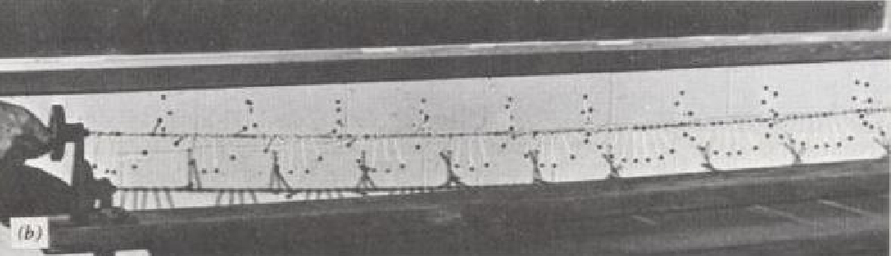
The sGe describes also the dynamics of the continuum limit of a sequence of neighbouring heavy pendula constrained to rotate around the same horizontal $x$-axis and coupled to each other through a torque spring [8] (see fig. 1); $\varphi(x,t)$ is the deviation angle from the lower vertical position at time $t$ of the pendulum having position $x$. One can model also the dissipative term $-\alpha\varphi_{t}$ of (1) by immersing the pendula in a linearly viscous fluid, and the forcing term $\gamma$ by assuming that a uniform, constant torque distribution is applied to the pendula.

This mechanical analog allows a qualitative comprehension of the main features of the solutions, e.g. of their instabilities. The constant solutions of (1) exist only for $|\gamma|\leq 1$ and are, mod $2\pi$,

$$\varphi^{s}(x,t)\equiv-\sin^{-1}\gamma,\qquad\qquad\varphi^{u}(x,t)\equiv\sin^{-1}\gamma\!+\!\pi.$$

(2)

If $|\gamma|\!<\!1$ the former is stable, the latter unstable, as they yield respectively local minima and maxima of the energy density

$$h:=\frac{\varphi_{t}^{2}}{2}+\frac{\varphi_{x}^{2}}{2}+\gamma\varphi-\cos\varphi.$$

(3)

In the mechanical analog they respectively correspond to configurations with all pendula hanging down or standing up. If $\gamma=\pm 1$ $\varphi^{s}=\varphi^{u}=\mp\pi/2\mbox{ (mod }2\pi)$, which is unstable because it is an inflection point for $h$.

In [5] we have performed a detailed analysis of travelling-wave solutions of (1). We briefly recall the framework adopted there and some of the results. Without loss of generality we can and shall assume $\gamma\geq 0$: if originally $\gamma\!<\!0$, we just need to replace $\varphi\to-\varphi$. Moreover, space or time translations transform any solution into a two-parameter family of solutions, so one can choose any of them as the family representative element; for travelling-wave solutions this reduces to translation of the only independent variable. In agreement with the conventions adopted in [5], we specify our travelling-wave Ansatz as follows:

$$\xi:=\pm x-t,\qquad\quad\varphi(x,t)\!=\!g(\xi)\!-\!\pi.$$

(4)

Replacing the Ansatz in (1) one obtains the first order ordinary differential equation

$$\alpha g^{\prime}=\gamma-\sin g.$$

(5)

We have already recalled the constant solutions. If $g^{\prime}$ is not identically zero, by integrating $d\xi=\alpha dg/(\gamma\!-\!\sin g)$ one finds

$$\xi-\xi_{0}=\int\limits^{\xi}_{\xi_{0}}d\xi=\alpha\int\limits^{g}_{g_{0}}\frac{ds}{\gamma-\sin s}$$

separately in each interval in which $g^{\prime}$ keeps its sign. This allows to determine the solution implicitly, namely the inverse $\xi(g)$.

If $\gamma\!\leq\!1$, as $g$ approaches respectively $\sin^{-1}\!\gamma$ or $\pi\!-\!\sin^{-1}\!\gamma$ (mod. $2\pi$) the denominator of the integrand goes to zero (linearly if $\gamma\!<\!1$, quadratically if $\gamma\!=\!1$) while keeping the same sign, and therefore the integral diverges, implying that the corresponding $\xi$ respectively goes either to $\pm\infty$, or to $\mp\infty$ [5]. In either case the range of $\xi(g)$ is the whole ${\mathbb{R}}$, implying that by taking the inverse one obtains $g(\xi)$ already in all the domain. If $\gamma\!>\!1$ the denominator of the integrand is positive for all $s\in{\mathbb{R}}$, so that the solution $g$ is strictly monotonic and linear-periodic, i.e. the sum of a linear and a periodic function, and

$$g(\xi+\Xi)=g(\xi)+2\pi,\qquad\qquad\Xi:=\alpha\int^{2\pi}_{0}\frac{ds}{\gamma-\sin s}.$$

(6)

Denoting as $\check{\varphi}^{\pm}$ the corresponding solutions with $\xi\!:=\!\pm\!x\!-\!t$, by (4) this implies

$$\check{\varphi}^{\pm}(x\!+\!\Xi,t)=\check{\varphi}^{\pm}(x,t)\pm 2\pi.$$

(7)

This behaviour is illustrated in fig. 2 by a picture of the corresponding configuration for the mechanical model of fig. 1.

$\check{\varphi}^{\pm}$ can be interpreted also as solutions of (1) on a circle of length $L=m\Xi$, for any $m\in{\mathbb{N}}$. The integer $m$ parameterizes different topological sectors: in the $m$-th the pendula chain twists around the circle $m$ times.

The purpose of this work is to determine in closed form the travelling-wave solutions (4) just described. We first transform eq. (5), with the help of the identities (18), into

$$4\alpha\frac{F^{\prime}}{1\!+\!F^{2}}=\gamma-4\frac{F(1\!-\!F^{2})}{(1\!+\!F^{2})^{2}}$$

by looking for $g$ in the form $g=4\tan^{-1}F$ and then into

$$2\alpha y^{\prime}=2y+\gamma(1\!+\!y^{2})$$

(8)

by looking for $F$ in the form $F=y\!+\!\sqrt{1\!+\!y^{2}}$. Note that diverging of $|y|$ at some point $\xi_{0}$ does not affect the continuity (and smoothness) of $g$ at $\xi_{0}$, even if the right limit is $\infty$ and the left one is $-\infty$, or viceversa: $y\to\pm\infty$ respectively implies $F\to\infty,0$ whence $g\to 0$ mod $2\pi$ in either case, which is compatible with a continuous $g$.

Below we solve for $y(\xi)$ explicitly. Putting all redefinitions together, we shall find solutions $\varphi$ through the formula

$$\varphi^{\pm}(x,t)\!=\!4\tan^{-1}\left[y(\pm x\!-\!t)\!+\!\sqrt{1\!+\!y^{2}(\pm x\!-\!t)}\right]\!-\!\pi.$$

(9)

Only if $\gamma\leq 1$ the solutions $y_{\pm}=-\!\gamma^{-1}\pm\sqrt{\gamma^{-2}\!-\!1}$ of the second degree equation $y^{2}\!+\!y2/\gamma\!+\!1=0$ are real and therefore give (real) constant solutions $y(\xi)\equiv y_{\pm}$ of (8), whence the already mentioned constant solutions $\varphi^{s},\varphi^{u}$ of (1). For nonconstant solutions (8) is equivalent to

$$d\xi=\frac{2\alpha}{\gamma}\frac{dy}{y^{2}+\frac{2}{\gamma}y+1}$$

(10)

separately in each interval where $y^{\prime}$ keeps its sign. The discussion of (10) depends now on the value of the discriminant $\Delta=4/\gamma^{2}\!-\!4$ of the equation $y^{2}\!+\!y2/\gamma\!+\!1=0$.

If $\gamma\!<\!1$, then $\Delta>0$, $y_{\pm}$ are real and different and (10) can be written as

$$d\xi=\frac{2\alpha}{\gamma}\frac{dy}{(y-y_{+})(y-y_{-})}=\frac{\alpha}{\sqrt{1\!-\!\gamma^{2}}}\left[\frac{dy}{y-y_{+}}-\frac{dy}{y-y_{-}}\right],$$

which is integrated to give the two families of solutions

$$y_{1}(\xi)=\frac{y_{+}+y_{-}e^{A(\xi\!-\!\xi_{0})}}{1+e^{A(\xi\!-\!\xi_{0})}},\qquad\qquad y_{2}(\xi)=\frac{y_{+}-y_{-}e^{A(\xi\!-\!\xi_{0})}}{1-e^{A(\xi\!-\!\xi_{0})}},$$

(11)

where $A:=(\sqrt{1\!-\!\gamma^{2}})\alpha^{-1}$ and $\xi_{0}$ is an integration constant. One easily checks that $y_{1}^{\prime},y_{2}^{\prime}$ (and therefore also $g_{1}^{\prime},g_{2}^{\prime}$) are respectively negative-, positive-definite; and that $\lim_{\xi\to\pm\infty}y_{i}(\xi)=y_{\mp}$ for both $i=1,2$. Using formulae (23-24) shown in the Appendix we thus find

$$\lim_{\xi\to\infty}F\big[y_{i}(\xi)\big]=F(y_{-})=\tan\theta,\qquad\qquad\lim_{\xi\to-\infty}F\big[y_{i}(\xi)\big]=F(y_{+})=\tan\left(\frac{\pi}{4}\!-\!\theta\right).$$

for both $i=1,2$, and mod $2\pi$ on one side a stricly decreasing $g_{1}(\xi)$ with

$$\lim_{\xi\to-\infty}g_{1}=\pi-\sin^{-1}\gamma,\qquad\qquad\lim_{\xi\to\infty}g_{1}=\sin^{-1}\gamma,$$

and on the other a stricly increasing $g_{2}(\xi)$ with

$$\lim_{\xi\to-\infty}g_{2}=\pi-\sin^{-1}\gamma,\qquad\qquad\lim_{\xi\to\infty}g_{2}=2\pi+\sin^{-1}\gamma.$$

As already noted, the singularity of $y_{2}$ at $\xi=\xi_{0}$ does not affect the continuity (and smoothness) of $g_{2}$. Correspondingly, mod $2\pi$

	$\displaystyle\lim_{x\to\mp\infty}\varphi^{\pm}_{1}=-\sin^{-1}\gamma\equiv\varphi^{s},\qquad\qquad\lim_{x\to\pm\infty}\varphi_{1}^{\pm}=-\pi+\sin^{-1}\gamma\equiv\varphi^{u},$		(12)
	$\displaystyle\lim_{x\to\mp\infty}\varphi_{2}^{\pm}=-\sin^{-1}\gamma\equiv\varphi^{s},\qquad\qquad\lim_{x\to\pm\infty}\varphi_{2}^{\pm}=\pi+\sin^{-1}\gamma\equiv\varphi^{u},$		(13)

therefore $\varphi_{1}^{\pm},\varphi_{2}^{\pm}$ are unstable solutions, as noted in [5].

If $\gamma=1$, then $\Delta=0$, $y_{\pm}=-1$ and (10) can be written as

$$d\xi=2\alpha\>\frac{dy}{(y+1)^{2}}=-2\alpha\>d\!\left[\frac{1}{y+1}\right],$$

which is integrated to give

$$y(\xi)=-\left[1+\frac{2\alpha}{\xi\!-\!\xi_{0}}\right].$$

(14)

This implies, with the help of (25),

$$\lim_{\xi\to\pm\infty}y(\xi)=-1,\qquad\Rightarrow\qquad\lim_{\xi\to\pm\infty}F\big[y(\xi)\big]=\sqrt{2}\!-\!1=\tan\frac{\pi}{8},$$

whereas again the singularity of $y$ at $\xi=\xi_{0}$ does not affect the continuity of $g$. As $y^{\prime}$, and therefore also $F^{\prime},g^{\prime}$, are positive-definite, one finds mod $2\pi$

$$\lim_{\xi\to-\infty}g=\frac{\pi}{2},\qquad\qquad\lim_{\xi\to\infty}g=\frac{5\pi}{2}$$

and, correspondingly,

$$\lim_{x\to\mp\infty}\varphi^{\pm}=-\frac{\pi}{2},\qquad\qquad\lim_{x\to\pm\infty}\varphi^{\pm}=\frac{3\pi}{2};$$

(15)

also these $\varphi^{\pm}$ are unstable, as noted in [5].

Finally, if $\gamma\!>\!1$, then $\Delta\!<\!0$, $y_{\pm}$ are complex conjugate and the denominator of (10) does not vanish for any value of $y$. Setting $w:=(y\gamma\!+\!1)/\sqrt{\gamma^{2}\!-\!1}$ (10) can be written as

$$d\xi=\frac{2\alpha}{\sqrt{\gamma^{2}\!-\!1}}\frac{dw}{1\!+\!w^{2}},$$

which is integrated to give $\xi\!-\!\xi_{0}=2\alpha\tan^{-1}w/\sqrt{\gamma^{2}\!-\!1}$, whence

$$y(\xi)=-\gamma^{-1}+\frac{1}{\sqrt{1\!-\!\gamma^{-2}}}\tan\left[\frac{\sqrt{\gamma^{2}\!-\!1}}{2\alpha}(\xi-\xi_{0})\right],$$

(16)

where $\xi_{0}$ is an integration constant. This is a periodic function with period

$$\Xi:=\frac{2\pi\alpha}{\sqrt{\gamma^{2}\!-\!1}},$$

(17)

and the latter is also the period occurring in (6). In fact, choosing $\xi_{0}=0$ for simplicity, we see that as $\xi$ varies from $-\Xi/2$ to $\Xi/2$ $y(\xi)$ varies from $-\infty$ to $\infty$, $F(\xi)$ varies from $0$ to $\infty$, $g(\xi)$ varies from $0$ to $2\pi$. By continuity of $g$ (which again is not affected by the singularity of $y$ at $\xi=\Xi(k\!+\!1/2)$ ($k\in{\mathbb{Z}}$), we thus find the behaviour (6). The corresponding solutions $\check{\varphi}^{\pm}$ fulfill (7), describe arrays of evenly-spaced kinks (see fig. 2) moving with velocity $\pm 1$ and are stable [5] (see also [7, 3]).

We first recall the trigonometric identities

$$\sin\!2\alpha\!=\!\frac{2\tan\!\alpha}{1\!+\!\tan^{2}\!\alpha},\quad\cos\!2\alpha\!=\!\frac{1\!-\!\tan^{2}\!\alpha}{1\!+\!\tan^{2}\!\alpha}\qquad\Rightarrow\qquad\sin\!4\alpha\!=\!\frac{4\tan\!\alpha(1\!-\!\tan^{2}\!\alpha)}{(1\!+\!\tan^{2}\!\alpha)^{2}}.$$

(18)

Given $\gamma\!\in\![0,1]$, let $\theta\!:=\!\frac{1}{4}\sin^{-1}\!\gamma\in\![0,\frac{\pi}{8}]$. Then $\gamma=\sin 4\theta$, $\sqrt{1\!-\!\gamma^{2}}=\cos 4\theta$ and, using the bisection formulae,

	$\displaystyle\sqrt{1\!+\!\sqrt{1\!-\!\gamma^{2}}}=\sqrt{1\!+\!\cos 4\theta}=\sqrt{2}\cos 2\theta,$		(19)
	$\displaystyle\sqrt{1\!-\!\sqrt{1\!-\!\gamma^{2}}}=\sqrt{1\!-\!\cos 4\theta}=\sqrt{2}\sin 2\theta,$		(20)

whence in turn

	$\displaystyle\sqrt{2}\!-\!\sqrt{1\!+\!\sqrt{1\!-\!\gamma^{2}}}=\sqrt{2}(1\!-\!\cos 2\theta)=2\sqrt{2}\sin^{2}\theta,$		(21)
	$\displaystyle\sqrt{2}\!-\!\sqrt{1\!-\!\sqrt{1\!-\!\gamma^{2}}}=\sqrt{2}(1\!-\!\sin\!2\theta)=\sqrt{2}\left[1\!-\!\cos\!\left(\frac{\pi}{2}\!-\!2\theta\right)\!\right]=2\sqrt{2}\sin^{2}\left(\frac{\pi}{4}\!-\!\theta\right).\qquad\quad$		(22)

Hence, using also the sinus duplication formula, we end up with

	$\displaystyle F(y_{+})$	$\displaystyle=$	$\displaystyle\frac{\sqrt{1\!-\!\sqrt{1\!-\!\gamma^{2}}}}{\gamma}\left[\sqrt{2}\!-\!\sqrt{1\!-\!\sqrt{1\!-\!\gamma^{2}}}\right]=\frac{4\sin 2\theta\sin^{2}\left(\frac{\pi}{4}\!-\!\theta\right)}{\sin 4\theta}$		(23)
		$\displaystyle=$	$\displaystyle\frac{2\sin^{2}\left(\frac{\pi}{4}\!-\!\theta\right)}{\cos 2\theta}=\frac{2\sin^{2}\left(\frac{\pi}{4}\!-\!\theta\right)}{\sin\left(\frac{\pi}{2}\!-\!2\theta\right)}=\frac{\sin\left(\frac{\pi}{4}\!-\!\theta\right)}{\cos\left(\frac{\pi}{4}\!-\!\theta\right)}=\tan\left(\frac{\pi}{4}\!-\!\theta\right),$
	$\displaystyle F(y_{-})$	$\displaystyle=$	$\displaystyle\frac{\sqrt{1\!+\!\sqrt{1\!-\!\gamma^{2}}}}{\gamma}\left[\!\sqrt{2}\!-\!\sqrt{1\!+\!\sqrt{1\!-\!\gamma^{2}}}\right]\!=\frac{4\cos\!2\theta\sin^{2}\!\theta}{\sin\!4\theta}=\frac{2\sin^{2}\!\theta}{\sin\!2\theta}=\tan\!\theta.\qquad$		(24)

If we choose $\gamma\!=\!1$ in (21) and use the sinus duplication formula we find as another consequence

$$\sqrt{2}\!-\!1=2\sqrt{2}\sin^{2}\left(\frac{\pi}{8}\right)=\frac{2\sin^{2}\left(\frac{\pi}{8}\right)}{\sin\left(\frac{\pi}{4}\right)}=\frac{\sin\frac{\pi}{8}}{\cos\frac{\pi}{8}}=\tan\frac{\pi}{8}.$$

(25)

References

- [1] A. Barone, G. Paternó, Physics and Applications of the Josephson Effect, Wiley-Interscience, New-York, 1982; and references therein.
- [2] P. l. Christiansen, A. C. Scott, M. P. Sorensen, Nonlinear Science at the Dawn of the 21st Century, Lecture Notes in Physics 542, Springer, 2000.
- [3] See e.g.: A. C. Scott, F. Y. F. Chu, and D. W. McLaughlin, The soliton: a new concept in applied science, Proc. IEEE 61 (1973), 1443-1483.
- [4] A. D’Anna, M. De Angelis, G. Fiore, Towards soliton solutions of a perturbed sine-Gordon equation, Rend. Acc. Sc. Fis. Mat. Napoli LXXII (2005), 95-110. math-ph/0507005
- [5] G. Fiore, Soliton and other travelling-wave solutions for a perturbed sine-Gordon equation, Preprint 05-49 Dip. Matematica e Applicazioni, Univ. “Federico II”, e DSF/42-2005. math-ph/0512002.
- [6] Josephson B. D. Possible new effects in superconductive tunneling, Phys. Lett. 1 (1962), 251-253; The discovery of tunneling supercurrents, Rev. Mod. Phys. B 46 (1974), 251-254; and references therein.
- [7] A. C. Scott, A nonlinear Klein-Gordon Equation. Am. J. Phys. 37 (1969), 52-61.
- [8] A. C. Scott, Active and Nonlinear Wave Propagation in Electronics. Wiley-Interscience, New-York, 1970, Chapters 2,5.
- [9] J.L. Shohet, B.R. Barmish, H.K. Ebraheem, and A.C. Scott, The sine-Gordon equation in reversed-field pinch experiments, Physics of Plasmas 11 (2004), 3877-3887.