Homogenization for Inertial Particles in a Random Flow

G. A. Pavliotis Thanks: Department of Mathematics, Imperial College London, London SW7˜2AZ, UK
(g.pavliotis@imperial.ac.uk) A. M. Stuart Thanks: Mathematics Institute, Warwick University, Coventry, CV4˜7AL, UK
(stuart@maths.warwick.ac.uk). K.C. Zygalakis Thanks: Mathematics Institute, Warwick University, Coventry, CV4˜7AL, UK
(zygk@maths.warwick.ac.uk).

Abstract

We study the problem of homogenization for inertial particles moving in a time dependent random velocity field and subject to molecular diffusion. We show that, under appropriate assumptions on the velocity field, the large–scale, long–time behavior of the inertial particles is governed by an effective diffusion equation for the position variable alone. This is achieved by the use of a formal multiple scales expansion in the scale parameter. The expansion relies on the hypoellipticity of the underlying diffusion. An expression for the diffusivity tensor is found and various of its properties are studied. The results of the formal multiscale analysis are justified rigorously by the use of the martingale central limit theorem. Our theoretical findings are supported by numerical investigations where we study the parametric dependence of the effective diffusivity on the various non–dimensional parameters of the problem.

1 Introduction

Inertial particles play an important role in various applications in science and engineering. Examples include planet formation, particle aggregation in rotating flows, atmosphere/ocean science (in particular rain initiation [10, 35]), chemical engineering. The prominent role that inertial particles play in various scientific and industrial applications has triggered many theoretical investigations, see for example [21, 24] and the references therein.

The starting point for many theoretical investigations concerning inertial particles is Stokes’ law which says that the force exerted by the fluid on the particle is proportional to the difference between the background fluid velocity and the particle velocity:

F_{\tiny{s}}(t)\propto\Bigl(v(x(t),t)-\dot{x}\Bigr).

(1)

Various extensions of this basic model have been considered in the literature, in particular by Maxey and collaborators [21, 22, 23, 24, 34, 39]. In this work we will restrict ourselves to the analysis of particles subject to a force of the form (1), together with additional molecular bombardment.

In principle the fluid velocity $v(x,t)$ satisfies either the Euler or the Navier Stokes equations and it is obtained through direct numerical simulations (DNS). The solution of a Newtonian particle governed by force law (1) coupled to either the Euler or Navier–Stokes equations is analytically difficult to study and computationally expensive. It is hence useful to consider $v(x,t)$ in (1) to be a given random field $v(x,t)$ which mimics some of the features of velocity fields obtained from DNS; one can consider, for example, random fields whose energy spectrum is consistent with that of velocity fields obtained from DNS. The qualitative study of Newtonian particles governed by (1) for given (random) velocity fields is very similar to the theory of turbulent diffusion [19], which has been primarily developed in the case $\tau=0$ . However, relatively little is known about the properties of solutions in the inertial case. It is important, therefore, to consider simplified models for the velocity field $v(x,t)$ which render the particle dynamics amenable to rigorous mathematical analysis and careful numerical investigations.

A model for the motion of inertial particles in two dimensions was introduced in [37] and analyzed in a series of papers [12, 17, 26, 27, 28, 31, 36]. This model consists of motion in a force field comprised of a contribution from Stokes’ law together with molecular bombardment; the velocity field is a Gaussian, Markovian, divergence–free random field. This gives the equations

	$\tau\ddot{x}(t)=v(x(t),t)-\dot{x}(t)+\sigma\xi(t),$		(2a)
	$v(x,t)=\nabla^{\bot}\phi(x,t),$		(2b)
	$\frac{\partial\phi}{\partial t}=A\phi+\sqrt{Q}\zeta(x,t).$		(2c)

The parameter $\tau$ is the Stokes number, which is a non–dimensional measure of the particle inertia (essentially it is the particle relaxation time). The molecular diffusion coefficient is given by $\sigma\geq 0$ , $\xi(t)$ is white noise in ${\mathbb{R}}^{2}$ , $\zeta(x,t)$ is space–time Gaussian white noise and $A,\,Q$ are appropriate positive, self–adjoint operators. Gaussian velocity fields of the form (2c) have been considered by various authors in the past, in particular in the context of passive advection. See for example [2] and the references therein. The usefulness of random velocity fields of the form (2c) in simulations is that, by choosing the operators $A$ and $Q$ appropriately, we can generate random velocity fields with a given energy spectrum, thus creating caricatures of realistic turbulent flows. Generalizations to arbitrary dimension $d$ are also possible

Various qualitative properties of the system (2) have been studied, such as existence and uniqueness of solutions and existence of a random attractor [36]. Furthermore, various limits of physical interest have been studied: rapid decorrelation in time (Kraichnan) limits [17, 26, 27].

Diffusive scaling limits (homogenization) were studied for time independent, periodic in space velocity fields; thus the model is obtained from (2a) with $v(x,t)=v(x)$ only [12, 28, 31]. In these three papers it was shown that the rescaled process

x^{\epsilon}(t):=\epsilon x(t/\epsilon^{2})

(3)

converges in distribution in the limit as $\epsilon\rightarrow 0$ to a Brownian motion with a nonnegative definite effective diffusivity ${\mathcal{K}}$ . Various properties of the effective diffusivity , in particular, the dependence of ${\mathcal{K}}$ on the parameters of the problem $\tau,\,\sigma$ were studied by means of formal asymptotics and extensive numerical simulations. The purpose of this paper is to carry out a similar analysis for the model problem (2) where the velocity field is time-dependent.

When $\tau=0$ , i.e. the particle inertia is negligible, the equation of motion (2a) becomes

\dot{x}(t)=v(x(t),t)+\sigma\xi(t).

(4)

This equation has been studied extensively in the literature [11, 19]. The homogenization problem for (4) with velocity fields of the form (2b),(2c) was studied in [3]. There it was shown that the rescaled process (3), with $x(t)$ being the solution of (4) and $v(x,t)$ being a finite dimensional truncation of solutions to (2b),(2c), converges in distribution to a Brownian motion with a positive definite covariance matrix, the effective diffusivity.

In this paper we will show that a similar result holds for the inertial particles problem. That is, we consider the diffusive rescaling (3) for solutions to (2) with $v(x,t)$ being a Galerkin truncation of (2c). We show, first with the aid of formal multiple scale expansions and then rigorously, that the rescaled processes converges to a Brownian motion and we derive a formula for the effective diffusion tensor. We study various properties of the effective diffusivity as well as some scaling limits of physical interest. Furthermore, we analyze the dependence of the effective diffusivity ${\mathcal{K}}$ on the various parameters of the problem through numerical simulations. In particular, we show that the effective diffusivity depends on the Stokes number $\tau$ in a very complicated, highly nonlinear way; this leads to various interesting, physically motivated, questions.

The generator of the Markov diffusion process corresponding to (2) is not a uniformly elliptic operator, as in the case of passive tracers, but a degenerate, hypoelliptic operator. This renders the proof of the homogenization theorem for (2) quite involved, since rather sophisticated tools from the spectral theory of hypoelliptic operators are required–see the Appendix.

The rest of the paper is organized as follows. In Section 2 we introduce the exact model that we will analyze and present some of its properties. In Section 3 we use the method of multiple scales to derive the homogenized equation. In Section 4 we study simultaneously the problems of homogenization and rapid decorrelation in time. In Section 5 we present the results of numerical simulations. Section 6 is reserved for conclusions. The rigorous homogenization theorem is stated and proved in the Appendix.

2 The Model

We will study the following model for the motion of an inertial particle in ${\mathbb{R}}^{d}$ [24]

\tau\ddot{x}(t)=v(x(t),t)-\dot{x}(t)+\sigma\xi(t),

(5)

where $\tau,\,\sigma>0$ and $\xi(t)$ is a standard white noise process on ${\mathbb{R}}^{d}$ , i.e. a mean zero generalized Gaussian process with

\langle\xi_{i}(t)\xi_{j}(s)\rangle=\delta_{ij}\delta(t-s),\quad i,j=1,\dots d.

The velocity field $v(x,t)$ is of the form

v(x,t)=F(x)\mu(t),

(6)

where for each fixed $x$ , $F(x):{\mathbb{R}}^{n}\rightarrow{\mathbb{R}}^{d}$ is an $n\times d$ matrix smooth and periodic as a function of $x$ , and $\mu(t)$ is a stationary generalized Ornstein–Uhlenbeck process on ${\mathbb{R}}^{n}$ :

\dot{\mu}(t)=-\frac{1}{\delta}A\mu(t)+\frac{1}{\delta}\sqrt{\Lambda}\zeta(t).

(7)

Here $\zeta(t)$ is a standard Gaussian white noise process on $\mathbb{R}^{n}$ , which is independent from $\xi(t)$ , $\delta>0$ and $A,\,\Lambda$ are positive definite $n\times n$ matrices. The parameter $\delta$ controls the correlation time of the Ornstein–Uhlenbeck process $\xi(t)$ . We remark that one can construct a velocity field (6) through a finite dimensional truncation of (2c). Notice however that we do not assume that the velocity field $v(x,t)$ is incompressible as such an assumption is not needed for the analysis. We will, however, restrict ourselves to incompressible velocity fields when studying the problem numerically in Section 5, as this case is physically interesting.

It is sometimes more convenient for the subsequent analysis to consider the rescaled OU process $\eta(t)=\sqrt{\delta}\mu(t)$ . Written in terms of $\eta(t)$ , the equations that govern the motion of inertial particles become

	$\tau\ddot{x}(t)=\frac{F(x(t))\eta(t)}{\sqrt{\delta}}-\dot{x}(t)+\sigma\xi(t),$		(8a)
	$\dot{\eta}(t)=-\frac{1}{\delta}A\eta(t)+\sqrt{\frac{\Lambda}{\delta}}\zeta(t),$		(8b)

The velocity field that appears in (8a) is a mean zero stationary ¹¹ 1 For appropriately chosen initial conditions. Gaussian random field with correlation time $\delta$ . It is possible to show [26] that in the limit as $\delta\rightarrow 0$ (the rapid decorrelation in time limit) the solution of (8a) converges pathwise to the solution of

\tau\ddot{x}(t)=F(x(t))A^{-1}\sqrt{\Lambda}\zeta(t)-\dot{x}(t)+\sigma\xi(t).

(9)

The Kraichnan–like velocity field

v(x,t)=F(x)A^{-1}\sqrt{\Lambda}\zeta(t)

is mean zero, Gaussian, and delta–correlated in time. We will refer to (8) as the colored velocity field model and to (9) as the white velocity field model.

In this paper we will be mostly concerned with the diffusive limit of solutions to (8) and (9) . That is, we will consider the rescaled process (3) and study the limit as $\epsilon\rightarrow 0$ . A natural question is whether the homogenization ( $\epsilon\rightarrow 0$ ) and rapid decorrelation in time ( $\delta\rightarrow 0$ ) limits commute. We answer this question in the affirmative through using formal asymptotics as well as through numerical investigations.

3 Multiple Scales Expansion for Effective Diffusivities

In this section we will derive the homogenized equation which describes the motion of inertial particles at large length and time scales for both the colored and white noise velocity fields. The derivation of the homogenized equation is based on multiscale/homogenization techniques [1]. We refer to [30] for a recent pedagogical introduction to such methods.

3.1 Homogenization for the colored velocity field

We start by rescaling the equations of motion (8) according to $t\mapsto t/\epsilon^{2}$ , $x\mapsto x/\epsilon$ . Using the fact that for any white noise process we have that $\xi(ct)=\frac{1}{\sqrt{c}}\xi(t)$ in law we obtain:


$\displaystyle\tau\epsilon^{2}\ddot{x}^{\epsilon}$	$\displaystyle=$	$\displaystyle\frac{1}{\epsilon}F\left(\frac{x^{\epsilon}}{\epsilon}\right)\frac{\eta^{\epsilon}}{\sqrt{\delta}}-\dot{x}^{\epsilon}+\sigma\xi,$	(10a)
$\displaystyle\dot{\eta^{\epsilon}}$	$\displaystyle=$	$\displaystyle-\frac{1}{\epsilon^{2}}\frac{A}{\delta}\eta^{\epsilon}+\frac{1}{\epsilon}\sqrt{\frac{\Lambda}{\delta}}\zeta.$	(10b)

We now introduce two new variables $y^{\epsilon}=\sqrt{\tau}\epsilon\dot{x}^{\epsilon}$ and $z^{\epsilon}=x^{\epsilon}/\epsilon$ and write the above equations as a first order system:


$\displaystyle dx^{\epsilon}(t)$	$\displaystyle=$	$\displaystyle\frac{1}{\sqrt{\tau}\epsilon}y^{\epsilon}(t)\,dt,$	(11a)
$\displaystyle dy^{\epsilon}(t)$	$\displaystyle=$	$\displaystyle\frac{1}{\epsilon^{2}\sqrt{\tau}}\frac{F(z^{\epsilon}(t))\eta^{\epsilon}(t)}{\sqrt{\delta}}\,dt-\frac{1}{\tau\epsilon^{2}}y^{\epsilon}(t)\,dt+\frac{\sigma}{\sqrt{\tau}\epsilon}\,dB(t),$	(11b)
$\displaystyle dz^{\epsilon}(t)$	$\displaystyle=$	$\displaystyle\frac{1}{\sqrt{\tau}\epsilon^{2}}y^{\epsilon}(t)\,dt,$	(11c)
$\displaystyle d\eta^{\epsilon}(t)$	$\displaystyle=$	$\displaystyle-\frac{1}{\epsilon^{2}}\frac{A}{\delta}\eta^{\epsilon}(t)\,dt+\frac{1}{\epsilon}\sqrt{\frac{\Lambda}{\delta}}\,dW(t),$	(11d)

with the understanding that $z^{\epsilon}\in\mathbb{T}^{d},\,x^{\epsilon},y^{\epsilon}\in\mathbb{R}^{d},\,\eta^{\epsilon}\in\mathbb{R}^{n}$ and with $\xi(t)=\dot{B}(t),\,\zeta(t)=\dot{W}(t)$ , $B(t)$ and $W(t)$ being standard Brownian motions on ${\mathbb{R}}^{d}$ and ${\mathbb{R}}^{n}$ , respectively. The SDEs (11) clearly exhibit the two time scales $\mathcal{O}(\epsilon)$ (for $x^{\epsilon}$ ) and $\mathcal{O}(\epsilon^{2})$ (for $(y^{\epsilon},z^{\epsilon},\eta^{\epsilon})$ ). Our purpose is to homogenize over the fast variables $(y^{\epsilon},z^{\epsilon},\eta^{\epsilon})$ to obtain a closed equation which governs the evolution of $x(t)$ , and is valid for $\epsilon\ll 1$ .

3.1.1 Multiscale expansion

Let $X^{x,y,z,\eta}_{t}:=\{x^{\epsilon}(t),y^{\epsilon}(t),z^{\epsilon}(t),\eta^{\epsilon}(t)\}$ denote the solution of (11) starting at $\{x,\,y,\,z,\,\eta\}$ and let $f:{\mathbb{R}}^{d}\times{\mathbb{R}}^{d}\times{\mathbb{T}}^{d}\times{\mathbb{R}}^{n}\mapsto{\mathbb{R}}$ be a smooth function. Then the observable $u^{\epsilon}(x,y,z,\eta,t)=\mathbb{E}f(X^{x,y,z,\eta}_{t})$ satisfies the backward Kolmogorov equation associated with the rescaled process:

$\displaystyle\frac{\partial u^{\epsilon}}{\partial t}$	$\displaystyle=$	$\displaystyle\frac{1}{\epsilon}\left(\frac{1}{\sqrt{\tau}}y\cdot\nabla_{x}\right)u^{\epsilon}+\frac{1}{\epsilon^{2}}\left[\frac{1}{\sqrt{\tau}}y\cdot\nabla_{z}+\frac{1}{\sqrt{\tau}}\frac{F(z)\eta}{\sqrt{\delta}}\cdot\nabla_{y}\right.$	(12)
		$\displaystyle\left.+\left(-\frac{A}{\delta}\eta\cdot\nabla_{\eta}+\frac{\Lambda}{2\delta}:\nabla_{\eta}\nabla_{\eta}\right)+\frac{1}{\tau}\left(-y\cdot\nabla_{y}+\frac{\sigma^{2}}{2}\Delta_{y}\right)\right]u^{\epsilon}$
	$\displaystyle=:$	$\displaystyle\left(\frac{1}{\epsilon^{2}}\mathcal{L}_{0}+\frac{1}{\epsilon}\mathcal{L}_{1}\right)u^{\epsilon},\ \text{with}\ \ u^{\epsilon}\|_{t=0}=f.$

Here:


$\displaystyle\mathcal{L}_{0}$	$\displaystyle:=$	$\displaystyle\frac{1}{\sqrt{\tau}}\left(y\cdot\nabla_{z}+\frac{F(z)\eta}{\sqrt{\delta}}\cdot\nabla_{y}\right)+\frac{1}{\tau}\mathcal{L}_{OU,y}+\frac{1}{\delta}\mathcal{L}_{OU,\eta},$	(13a)
$\displaystyle\mathcal{L}_{1}$	$\displaystyle:=$	$\displaystyle\frac{1}{\sqrt{\tau}}y\cdot\nabla_{x},$	(13b)
$\displaystyle\mathcal{L}_{OU,\eta}$	$\displaystyle:=$	$\displaystyle-A\eta\cdot\nabla_{\eta}+\frac{\Lambda}{2}:\nabla_{\eta}\nabla_{\eta},$	(13c)
$\displaystyle\mathcal{L}_{OU,y}$	$\displaystyle:=$	$\displaystyle-y\cdot\nabla_{y}+\frac{\sigma^{2}}{2}\Delta_{y}.$	(13d)

We use the subscript $OU$ on the last two operators to emphasize that they are the generators of Ornstein-Uhlenbeck processes in $\eta$ and $y$ respectively. The operator $\mathcal{L}_{0}$ is the generator of the Markov process $\{z(t),y(t),\eta(t)\}\in{\mathbb{T}}^{d}\times{\mathbb{R}}^{d}\times{\mathbb{R}}^{n}$ :


$\displaystyle dz(t)$	$\displaystyle=$	$\displaystyle\frac{1}{\sqrt{\tau}}y(t)\,dt,$	(14a)
$\displaystyle dy(t)$	$\displaystyle=$	$\displaystyle\frac{1}{\sqrt{\tau}}\frac{F(z(t))\eta(t)}{\sqrt{\delta}}\,dt-\frac{1}{\tau}y(t)\,dt+\frac{\sigma}{\sqrt{\tau}}\,dB(t),$	(14b)
$\displaystyle d\eta(t)$	$\displaystyle=$	$\displaystyle-\frac{A}{\delta}\eta(t)\,dt+\sqrt{\frac{\Lambda}{\delta}}\,dW(t).$	(14c)

In the Appendix we prove that the Markov process $\{z(t),y(t),\eta(t)\}$ given by (14) is geometrically ergodic. Hence, there exists a unique invariant measure with smooth density $\rho(z,y,\eta)$ which is the solution of the stationary Fokker–Planck equation

\mathcal{L}_{0}^{\ast}\rho=-\frac{1}{\sqrt{\tau}}\left(y\cdot\nabla_{z}\rho+F(z)\eta\cdot\nabla_{y}\rho\right)+\frac{1}{\tau}\mathcal{L}_{OU,y}^{*}\rho+\frac{1}{\delta}\mathcal{L}_{OU,\eta}^{*}\rho=0.

(15)

Here

\mathcal{L}_{OU,y}^{*}\cdot:=\nabla_{y}\cdot(y\cdot)+\frac{\sigma^{2}}{2}\Delta_{y}\cdot\quad\mbox{and}\quad\mathcal{L}_{OU,\eta}^{*}\cdot:=\nabla_{\eta}\cdot(A\eta\cdot)+\frac{\Lambda}{2}:\nabla_{\eta}\nabla_{\eta}\cdot

are the formal $L^{2}$ –adjoints of $\mathcal{L}_{OU,y}$ and $\mathcal{L}_{OU,\eta}$ , respectively. The invariant density $\rho(z,y,\eta)$ is a periodic function of $z$ and decays rapidly as $\|z\|,\,\|y\|\rightarrow\infty$ .

In the Appendix we also prove that the operator ${\mathcal{L}}^{*}_{0}$ (equipped with boundary conditions described above) has compact resolvent in the appropriate function space. Consequently, Fredholm theory applies: the null space of the generator $\mathcal{L}_{0}$ is one dimensional and consists of constants in $z,y,\eta$ . (See the Appendix). Moreover the equation $\mathcal{L}_{0}f=g$ , has a unique (up to constants) solution if and only if

\left\langle g\right\rangle_{\rho}:=\int_{\mathbb{X}}g(y,z,\eta)\rho(y,z,\eta)\,dX=0

where $\mathbb{X}:=\mathbb{T}^{d}\times\mathbb{R}^{d}\times\mathbb{R}^{n}$ and $dX:=dydzd\eta$ . We assume that that the average of the velocity with respect to the invariant density $\rho$ vanishes:

\left\langle F(z)\eta\right\rangle_{\rho}=0.

(16)

This is natural because it removes any effective drift making a purely diffusive scaling natural. The identity $\int_{\mathbb{X}}y\big(\mathcal{L}_{0}^{\ast}\rho(y,z,\eta)\big)\,dX=0$ implies that

\int_{\mathbb{X}}\big(\mathcal{L}_{0}y\big)\rho(y,z,\eta)\,dX=0.

Consequently:

\int_{\mathbb{X}}\left(\frac{1}{\sqrt{\tau}}\frac{F(z)\eta}{\sqrt{\delta}}-\frac{1}{\tau}y\right)\rho(y,z,\eta)\,dX=0

Thus, the centering condition (16) is equivalent to:

\left\langle y\right\rangle_{\rho}=0.

(17)

Let us now proceed with the derivation of the homogenized equation. We look for a solution of (12) in the form of a power series in $\epsilon$ :

u^{\epsilon}=u_{0}(x,y,z,\eta,t)+\epsilon u_{1}(x,y,z,\eta,t)+\epsilon^{2}u_{2}(x,y,z,\eta,t)+\ldots

(18)

with $u_{i}=u_{i}(x,y,z,\eta,t),\,i=1,2,\ldots$ being $1$ –periodic in $z$ . We substitute (18) into (12) and obtain the following sequence of equations:


$\displaystyle-\mathcal{L}_{0}u_{0}$	$\displaystyle=$	$\displaystyle 0,$	(19a)
$\displaystyle-\mathcal{L}_{0}u_{1}$	$\displaystyle=$	$\displaystyle\mathcal{L}_{1}u_{0},$	(19b)
$\displaystyle-\mathcal{L}_{0}u_{2}$	$\displaystyle=$	$\displaystyle\mathcal{L}_{1}u_{1}-\frac{\partial u_{0}}{\partial t},$	(19c)

From (19a), we deduce that the first term in the expansion is independent of the fast variables $z,\,y,\,\eta$ , i.e. $u_{0}=u(x,t)$ . Now equation (19b) becomes:

-\mathcal{L}_{0}u_{1}=\frac{1}{\sqrt{\tau}}y\cdot\nabla_{x}u.

We can solve this by using separation of variables²² 2 In principle we should also add a term which is in the null space of ${\mathcal{L}}_{0}$ . It is easy to show, however, that this term does not affect the homogenized equation and for simplicity we set it equal to $0$ .:

u_{1}=\Phi(y,z,\eta)\cdot\nabla_{x}u,

with

-\mathcal{L}_{0}\Phi(y,z,\eta)=\frac{1}{\sqrt{\tau}}y.

(20)

This is the cell problem which is posed on $\mathbb{X}$ . Assumption (17) implies that the right hand side of the the above equation is centered with respect to the invariant measure of the fast process. Hence the equation is well posed (see the Appendix). The boundary conditions for this PDE are that $\Phi(y,z,\eta)$ is periodic in $z$ and that it belongs to $L^{2}(\mathbb{X},\rho(z,y,\eta)\,dzdyd\eta)$ , which implies sufficiently fast decay at infinity.

We now proceed with (19c). We apply the solvability condition to obtain:

	$\displaystyle\frac{\partial u_{0}}{\partial t}$	$\displaystyle=$	$\displaystyle\left\langle\mathcal{L}_{1}u_{1}\right\rangle_{\rho}$		(21)
		$\displaystyle=$	$\displaystyle\frac{1}{\sqrt{\tau}}\left\langle y\otimes\Phi\right\rangle_{\rho}:\nabla_{x}\nabla_{x}u.$		(21)

Thus, the backward Kolmogorov equation which governs the dynamics on large scales is

\frac{\partial u}{\partial t}=\mathcal{K}:\nabla_{x}\nabla_{x}u,

(22)

where the effective diffusivity is given by

\mathcal{K}=\frac{1}{\sqrt{\tau}}\left\langle y\otimes\Phi\right\rangle_{\rho},

(23)

and where $\otimes$ denotes the tensor (or outer) product. Notice that only the symmetric part of the effective diffusivity $\mathcal{K}$ is relevant in the homogenized equation (22). However, the effective diffusivity $\mathcal{K}$ itself is non–symmetric in general. We define

sym({\mathcal{K}})=\frac{1}{2}({\mathcal{K}}+{\mathcal{K}}^{T})

3.1.2 The homogenization result

Equation (22) is the Backward Kolmogorov equation corresponding to a pure Brownian motion. We have the following result:

Result 3.1.

For $\epsilon\ll 1$ and $t=\mathcal{O}(1)$ the function $x^{\epsilon}(t)=\epsilon x(t/\epsilon^{2})$ , where $x(t)$ solves (8), is approximated by $X(t)$ solving

\dot{X}=\sqrt{2sym({\mathcal{K}})}\dot{\beta}.

(24)

with $X(0)=x(0),$ and where $\beta$ is a standard Brownian motion on $\mathbb{R}^{d}.$

A theorem, justifying the formal approximation leading to this result, is proved in the Appendix, using the martingale central limit theorem.

3.1.3 Properties of the effective diffusivity

In this subsection we show that the effective diffusivity is non negative. This implies that the homogenization equation is well posed. We can show this by using the Dirichlet form (Theorem 6.12 in [30]) which shows that, for every sufficiently smooth $f(z,y,\eta)$ ,

\int_{\mathbb{X}}f(-\mathcal{L}_{0}f)\rho\,dX=\frac{\sigma^{2}}{2\tau}\left\langle|\nabla_{y}f|^{2}\right\rangle_{\rho}+\frac{1}{2\delta}\left\langle(\nabla_{\eta}f)^{T}\Lambda(\nabla_{\eta}f)\right\rangle_{\rho}.

(25)

Now let $\Phi$ be the solution of the Poisson equation (20) and define $\phi^{\alpha}:=\alpha\cdot\Phi$ , where $\alpha\in{\mathbb{R}}^{d}$ is an arbitrary unit vector. The scalar field $\phi^{\alpha}$ satisfies the Poisson equation

-\mathcal{L}_{0}\phi^{\alpha}=\frac{1}{\sqrt{\tau}}\alpha\cdot y.

We combine (23) with (25), to calculate

$\displaystyle\alpha.\mathcal{K}\alpha$	$\displaystyle=$	$\displaystyle\frac{1}{\sqrt{\tau}}\int_{\mathbb{X}}(\alpha\cdot y)(\alpha\cdot\Phi)\rho\,dX$	(26)
	$\displaystyle=$	$\displaystyle\int_{\mathbb{X}}\phi^{\alpha}(-\mathcal{L}_{0}\phi^{\alpha})\rho\,dX$
	$\displaystyle=$	$\displaystyle\frac{\sigma^{2}}{2\tau}\left\langle\|\nabla_{y}\phi^{\alpha}\|^{2}\right\rangle_{\rho}+\frac{1}{2\delta}\left\langle(\nabla_{\eta}\phi^{\alpha})^{T}\Lambda(\nabla_{\eta}\phi^{\alpha})\right\rangle_{\rho}$
	$\displaystyle\geq$	$\displaystyle 0,$

since $\Lambda$ is a positive definite matrix. Thus the following results holds:

Result 3.2.

The effective diffusivity matrix $\mathcal{K}$ given by (23) is positive semi-definite and thus the limiting backward Kolmogorov equation (22) is well posed.

Remark 3.1.

It is not entirely straightforward to check whether the centering condition (16) or, equivalently, (17) is satisfied or not, as we don’t have a formula for the invariant measure of the fast process–we only know that it exists. It is possible, however, to identify some general classes of flows $v(x,t)$ which satisfy (16) by using symmetry arguments. Consider for example the case of a parity invariant flow, i.e a flow satisfying the condition

F(-z)=-F(z).

(27)

It follows from (27) and (15) that the invariant density satisfies

\rho(y,z,\eta)=\rho(-y,-z,\eta).

(28)

It is easy to see now that (28) implies that (16) is satisfied. Hence, the centering condition is satisfied for velocity fields $v(x,t)$ that are odd functions of $x$ .

Remark 3.2.

Even if the centering condition is not satisfied, the large-scale, long-time dynamics of the inertial particle is still governed by an effective Brownian motion, provided that we study the problem in a frame co-moving with the mean flow. Indeed, if we denote by $V$ the mean flow, i.e.

V=\langle F(z)\eta\rangle_{\rho},

then the rescaled processed $x^{\epsilon}=\epsilon\left(x(t/\epsilon^{2})-Vt/\epsilon^{2}\right)$ converges in distribution to a Brownian motion with covariance matrix (the effective diffusivity) given by

{\mathcal{K}}=\frac{1}{\sqrt{\tau}}\left\langle\left(y-\sqrt{\frac{\tau}{\delta}}V\right)\otimes\Psi\right\rangle_{\rho}

(29)

with

-{\mathcal{L}}_{0}\Psi=\frac{1}{\sqrt{\tau}}\Bigl(y-\sqrt{\frac{\tau}{\delta}}V\Bigr),\quad{\mathcal{L}}_{0}^{*}\rho=0.

(30)

3.2 Homogenization: the white noise velocity field

We can use the same multiscale techniques to study the diffusive scaling of (8a) for the white velocity field, equation (9):

\tau\ddot{x}(t)=F(x(t))A^{-1}\sqrt{\Lambda}\zeta(t)-\dot{x}+\sigma\xi(t).

After a similar calculation with the colored noise problem we find that the backward Kolmogorov equation which governs the dynamics on large scale is

\frac{\partial u}{\partial t}=\widehat{{\mathcal{K}}}:\nabla_{x}\nabla_{x}u,

(31)

where the effective diffusivity is given by

\widehat{{\mathcal{K}}}=\frac{1}{\sqrt{\tau}}\langle y\otimes\widehat{\Phi}\rangle_{\widehat{\rho}}.

(32)

Here

-\widehat{{\mathcal{L}}}_{0}\widehat{\Phi}(y,z)=\frac{1}{\sqrt{\tau}}y,\quad\widehat{\mathcal{L}}_{0}^{*}\widehat{\rho}=0,

(33)

with

\widehat{\mathcal{L}}_{0}:=\frac{1}{\sqrt{\tau}}y\cdot\nabla_{z}+\frac{1}{2\tau}F(z)A^{-1}\Lambda A^{-1}F^{T}(z):\nabla_{y}\nabla_{y}+\frac{1}{\tau}\mathcal{L}_{OU,y}.

(34)

The operator $\mathcal{L}_{OU,y}$ is defined in (13). We use the notation $\langle\rangle_{\widehat{\rho}}$ to denote averaging over ${\mathbb{T}}^{d}\times{\mathbb{R}}^{d}$ with respect to the invariant distribution $\widehat{\rho}$ .

3.2.1 The homogenization result

Equation (31) is the backward Kolmogorov equation corresponding to a pure Brownian motion. Hence we have the following result:

Result 3.3.

For $\epsilon<<1$ and $t=\mathcal{O}(1)$ the function $x^{\epsilon}(t)=\epsilon x(t/\epsilon^{2})$ , where $x(t)$ solves (9), is approximated by $X(t)$ solving

\dot{X}=\sqrt{2sym(\widehat{{\mathcal{K}}})}\dot{\beta},

(35)

with $X(0)=x(0),$ and where $\beta$ is a standard Brownian motion on $\mathbb{R}^{d}.$

This result can be justified rigorously by means of the martingale central limit theorem, as is done for the coloured noise case in the Appendix.

3.2.2 Properties of the effective diffusivity

As in the case of the colored velocity field, the covariance matrix of the limiting Brownian motion is nonnegative define. Indeed, let $\alpha\in{\mathbb{R}}^{d}$ be an arbitrary unit vector, define $\widehat{\phi}^{\alpha}:=\alpha\cdot\widehat{\Phi}$ and use the Dirichlet form (Theorem 6.12 in [30])

	$\displaystyle\alpha.\widehat{{\mathcal{K}}}\alpha$	$\displaystyle=$	$\displaystyle\frac{\sigma^{2}}{2\tau}\left\langle\|\nabla_{y}\widehat{\phi}^{\alpha}\|^{2}\right\rangle_{\widehat{\rho}}+\frac{1}{2\tau}\left\langle(\nabla_{y}\widehat{\phi}^{\alpha})^{T}F(z)A^{-1}\Lambda A^{-1}F(z)^{T}(\nabla_{y}\widehat{\phi}^{\alpha})\right\rangle_{\widehat{\rho}}$
		$\displaystyle\geq$	$\displaystyle 0.$

Thus we have the following result:

Result 3.4.

The effective diffusivity matrix $\widehat{{\mathcal{K}}}$ given by (32) is positive semi-definite and thus the associated backward Kolmogorov equation is well posed.

Remark 3.3.

An important observation is that the centering condition for the white noise problem is always satisfied. Indeed, let $\widehat{{\mathbb{X}}}:={\mathbb{T}}^{d}\times{\mathbb{R}}^{d}$ , $d\widehat{X}:=dzdy$ and use the identity

\int_{\widehat{\mathbb{X}}}y\widehat{{\mathcal{L}}}_{0}^{\ast}\widehat{\rho}(y,z)d\widehat{X}=0

together with integrations by parts to deduce that

\int_{\widehat{\mathbb{X}}}y\widehat{\rho}(y,z)d\widehat{X}=0.

This suffices for solvability of (33). Hence, the long–time, large–scale behavior of solutions to (9) is always diffusive. This is to be contrasted with the case of the colored velocity field, where an additional condition, equation (16), has to be imposed to ensure diffusive large scale dynamics.

4 White Noise Limit for the Effective Diffusivity

Consider the rescaled equation (10), and denote its solution by $x^{\delta,\epsilon}(t)$ . It is clear that if we first take the limit as $\delta\rightarrow 0$ and then the limit $\epsilon\rightarrow 0$ , then $x^{\delta,\epsilon}(t)$ converges to a Brownian motion with covariance matrix $\widehat{{\mathcal{K}}}$ given by eqn. (32), without having to impose any centering condition. A natural question arises as to what happens if we interchange the order with which we take the limits $\delta,\epsilon\to 0$ . In this section we show that the two limits commute under the additional assumption that the centering condition (16) is satisfied. In particular we have the following result:

Result 4.1.

Let $A,\Lambda$ be positive definite matrices that commute and assume that the centering condition (16) is satisfied. Then for $\delta\ll 1$ the effective diffusivity ${\mathcal{K}}$ from the colored noise model given by (23) admits the asymptotic expansion

{\mathcal{K}}=\widehat{{\mathcal{K}}}+\mathcal{O}(\sqrt{\delta}),

(36)

where $\widehat{{\mathcal{K}}}$ is given by (32).

The derivation of (36) is based on singular perturbation analysis of the cell problem (20) and of the stationary Fokker-Planck equation (15); see [29, 28, 14]. We start by writing the operator $\mathcal{L}_{0}$ defined in (13) in the form,

\mathcal{L}_{0}=\frac{1}{\delta}\mathcal{A}_{0}+\frac{1}{\sqrt{\delta}}\mathcal{A}_{1}+\mathcal{A}_{2},

(37)

with

\mathcal{A}_{0}=\mathcal{L}_{OU,\eta},\quad\mathcal{A}_{1}=\frac{1}{\sqrt{\tau}}F(z)\eta\cdot\nabla_{y},\quad\mathcal{A}_{2}=\frac{1}{\sqrt{\tau}}y\cdot\nabla_{z}+\frac{1}{\tau}\mathcal{L}_{OU,y}.

Of course, $\mathcal{L}_{0}^{\ast}$ is also of the form (37) with $\mathcal{A}_{j}$ replaced with $\mathcal{A}_{j}^{*},\,j=0,1,2$ .

Note that $\mathcal{A}_{0}$ is the generator of a $d$ -dimensional OU process. Hence, it has a one–dimensional null space which consists of constants in $\eta$ . Furthermore, the process generated by $\mathcal{A}_{0}$ is geometrically ergodic and its invariant measure is Gaussian. Since $A$ and $\Lambda$ commute, the density of the unique Gaussian invariant measure (i.e., the solution of the equation $\mathcal{A}_{0}^{*}\rho^{\eta}=0$ ) is

\rho^{\eta}=\frac{1}{Z}\exp\bigl(-\eta^{T}\Lambda^{-1}A\eta\bigr),

where $Z$ is the normalization constant.

Let $\Phi$ be the solution of (20). As before, we define $\phi^{\alpha}=\Phi\cdot\alpha$ for an arbitrary unit vector $\alpha\in{\mathbb{R}}^{d}$ . We have that

-\mathcal{L}_{0}\phi^{\alpha}=\frac{1}{\sqrt{\tau}}y\cdot\alpha,

(38)

that

\mathcal{L}_{0}^{\star}\rho=0

(39)

and that

\alpha\cdot{\mathcal{K}}\alpha=\frac{1}{\sqrt{\tau}}\langle\alpha\cdot y\phi^{\alpha}\rangle_{\rho}

(40)

Now we need to calculate the small $\delta$ asymptotics of $\phi^{\alpha}$ and $\rho$ .

4.1 Expansion for $\phi^{\alpha}$

We look for a solution of (38) in the form of a power series in $\sqrt{\delta}$ .

\phi^{\alpha}=\phi^{\alpha}_{0}+\sqrt{\delta}\phi^{\alpha}_{1}+\delta\phi^{\alpha}_{2}+\dots

We substitute the above into (38) to obtain the following sequence of equations


$\displaystyle-\mathcal{A}_{0}\phi^{\alpha}_{0}$	$\displaystyle=$	$\displaystyle 0,$	(41a)
$\displaystyle-\mathcal{A}_{0}\phi^{\alpha}_{1}$	$\displaystyle=$	$\displaystyle\mathcal{A}_{1}\phi^{\alpha}_{0},$	(41b)
$\displaystyle-\mathcal{A}_{0}\phi^{\alpha}_{2}$	$\displaystyle=$	$\displaystyle\mathcal{A}_{1}\phi^{\alpha}_{1}+\mathcal{A}_{2}\phi^{\alpha}_{0}+\frac{1}{\sqrt{\tau}}y\cdot\alpha.$	(41c)

From Equation (41a) we get that $\phi^{\alpha}_{0}=\phi^{\alpha}_{0}(z,y)$ . In order for equation (41b) to be well posed it is necessary that the right hand side of the equation is orthogonal to the null space of $\mathcal{A}_{0}^{*}$ , i.e. that

\left\langle\frac{1}{\sqrt{\tau}}F(z)\eta\cdot\nabla_{y}\phi_{0}^{\alpha}(z,y)\right\rangle_{\rho^{\eta}}=0,

which is satisfied, since the term to be averaged is linear in $\eta$ and $\rho^{\eta}$ is a mean zero Gaussian density. The solution of Equation (41b) is

\phi^{\alpha}_{1}=\frac{1}{\sqrt{\tau}}F(z)A^{-1}\eta\cdot\nabla_{y}\phi^{\alpha}_{0}+\widehat{\Psi}_{1}(z,y).

The solvability condition for (41c) gives

\displaystyle\left\langle\frac{1}{\tau}\eta^{T}\Big(F^{T}(z)\nabla_{y}\nabla_{y}\phi^{\alpha}_{0}F(z)A^{-1}\Big)\eta\right\rangle_{\rho^{\eta}}+\frac{1}{\sqrt{\tau}}y\cdot\nabla_{z}\phi^{\alpha}_{0}+\frac{1}{\tau}\mathcal{L}_{OU,y}\phi^{\alpha}_{0}+\frac{1}{\sqrt{\tau}}y\cdot\alpha=0.

We use the fact that

\langle\eta^{T}B\eta\rangle_{\rho^{\eta}}=\frac{1}{2}B:A^{-1}\Lambda\quad\forall\,B\in{\mathbb{R}}^{d\times d},

to obtain

-\widehat{\mathcal{L}}_{0}\phi^{\alpha}_{0}=\frac{1}{\sqrt{\tau}}y\cdot\alpha.

(42)

This is precisely the cell problem for the white noise velocity field, equation (33) projected along the direction $\alpha\in{\mathbb{R}}^{d}$ . Hence, the small $\delta$ expansion of the solution to (38) is

\phi^{\alpha}(z,y,\eta)=\phi^{\alpha}_{0}(z,y)+\sqrt{\delta}\left(\frac{1}{\sqrt{\tau}}F(z)A^{-1}\eta\cdot\nabla_{y}\phi^{\alpha}_{0}+\widehat{\Psi}_{1}(z,y)\right)+{\mathcal{O}}(\delta),

(43)

where $\phi^{\alpha}_{0}(z,y)$ is the solution to (42).

4.2 Expansion for $\rho$

We look for a solution of (39) in the form of a power series in $\sqrt{\delta}$

\rho=\rho_{0}+\sqrt{\delta}\rho_{1}+\delta\rho_{2}+\dots

We substitute this expansion into (39) and equate equal powers of $\delta$ to obtain the following sequence of equations.


$\displaystyle-\mathcal{A}_{0}^{*}\rho_{0}$	$\displaystyle=$	$\displaystyle 0,$	(44a)
$\displaystyle-\mathcal{A}_{0}^{*}\rho_{1}$	$\displaystyle=$	$\displaystyle\mathcal{A}_{1}^{*}\rho_{0},$	(44b)
$\displaystyle-\mathcal{A}_{0}^{*}\rho_{2}$	$\displaystyle=$	$\displaystyle\mathcal{A}_{1}^{}\rho_{1}+\mathcal{A}_{2}^{}\rho_{0}.$	(44c)

From the first equation we deduce that (abusing notation) $\rho_{0}(z,y,\eta)=\rho_{0}(z,y)\rho^{\eta}$ . The solvability condition for (44b) is satisfied since

-\int_{\mathbb{R}^{m}}\mathcal{A}_{1}^{*}\rho_{0}\,d\eta=\int_{\mathbb{R}^{m}}\frac{1}{\sqrt{\tau}}\Bigl(F(z)\eta\cdot\nabla_{y}\rho_{0}(z,y)\Bigr)\rho^{\eta}\,d\eta=0.

The solution of (44b) is

\rho_{1}(z,y,\eta)=\rho^{\eta}\left(\frac{1}{\sqrt{\tau}}F(z)A^{-1}\eta\cdot\nabla_{y}\rho_{0}(z,y)+\overline{\rho}_{1}(z,y)\right).

The solvability condition for (44c) is

\int_{{\mathbb{R}}^{m}}\left(\mathcal{A}_{1}^{*}\rho_{1}+\mathcal{A}_{2}^{*}\rho_{0}\right)\,d\eta=0.

(45)

We use the expressions for $\rho_{0}$ and $\rho_{1}$ to deduce that

\int_{{\mathbb{R}}^{m}}\mathcal{A}_{2}^{*}\rho_{0}(z,y,\eta)\,d\eta=-\frac{1}{\sqrt{\tau}}y\cdot\nabla_{z}\rho_{0}(z,y)+\frac{1}{\tau}\mathcal{L}_{OU,y}^{\ast}\rho_{0}(z,y).

and

\int_{{\mathbb{R}}^{m}}\mathcal{A}_{1}^{*}\rho_{1}\,d\eta=\frac{1}{2\tau}F(z)A^{-1}\Lambda A^{-1}F^{T}(z):\nabla_{y}\nabla_{y}\rho_{0}.

We substitute the above expressions in (45) to conclude that $\rho_{0}(z,y)$ satisfies

\widehat{\mathcal{L}}_{0}^{\star}\rho_{0}=0.

(46)

Consequently, $\rho_{0}(z,y)=\widehat{\rho}(z,y)$ , the solution of the second equation in (33). Thus, the small $\delta$ expansion of $\rho$ , the solution of (39) is

\rho=\widehat{\rho}(z,y)\rho^{\eta}+\sqrt{\delta}\rho^{\eta}\left(\frac{1}{\sqrt{\tau}}F(x)A^{-1}\eta\cdot\nabla_{y}\rho_{0}(z,y)+\overline{\rho}_{1}(z,y)\right)+{\mathcal{O}}(\delta).

(47)

4.3 Proof of Result 4.1

We have that

\alpha\cdot{\mathcal{K}}\alpha=\frac{1}{\sqrt{\tau}}\langle\alpha\cdot y\phi^{\alpha}\rangle_{\rho}.

(48)

In the previous subsections we expanded $\phi^{\alpha}$ and $\rho$ as

	$\displaystyle\phi^{\alpha}$	$\displaystyle=$	$\displaystyle\phi^{\alpha}_{0}+\sqrt{\delta}\phi^{\alpha}_{1}+\delta\phi^{\alpha}_{2}+\cdots$
	$\displaystyle\rho$	$\displaystyle=$	$\displaystyle\rho_{0}+\sqrt{\delta}\rho_{1}+\delta\rho_{2}+\dots$

and showed that

	$\displaystyle\phi^{\alpha}_{0}(x,y,\eta)$	$\displaystyle=$	$\displaystyle\phi_{0}^{\alpha}(x,y),$
	$\displaystyle\rho_{0}(x,y,\eta)$	$\displaystyle=$	$\displaystyle\rho^{\eta}\widehat{\rho}(x,y),$

where $\phi_{0}^{\alpha}={\widehat{\Phi}}\cdot\alpha$ and ${\widehat{\Phi}},{\widehat{\rho}}$ satisfy (33). Now if we substitute the series expansion in (48) we obtain:

\alpha\cdot{\mathcal{K}}\alpha=\frac{1}{\sqrt{\tau}}\langle\alpha\cdot y\phi_{0}^{\alpha}\rangle_{\rho^{\eta}\widehat{\rho}(x,y)}+\mathcal{O}(\sqrt{\delta}).

Since $\phi_{0}^{\alpha}$ does not depend on $\eta$ we can integrate over the $\eta$ variable and obtain

	$\displaystyle\alpha\cdot{\mathcal{K}}\alpha$	$\displaystyle=$	$\displaystyle\frac{1}{\sqrt{\tau}}\langle\alpha\cdot y\phi_{0}^{\alpha}\rangle_{\widehat{\rho}(x,y)}+\mathcal{O}(\sqrt{\delta}).$		(49)
		$\displaystyle=$	$\displaystyle\alpha\cdot\widehat{{\mathcal{K}}}\alpha+\mathcal{O}(\sqrt{\delta})$		(50)

Remark 4.1.

Thus we have shown that for $\delta\ll 1$ the effective diffusivity of the colored noise problem is approximately equal to that arising from the white noise problem up to terms of $\mathcal{O}(\delta),$ provided the centering condition is satisfied. It is straightforward to show that exactly the same result holds even when the centering condition is not satisfied. In this case the asymptotic analysis is done for equations (29) and (30); the effective drift $V$ vanishes in the limit $\delta\rightarrow 0$ .

5 Numerical Investigations

In this section we study the dependence of the effective diffusivity (23) or (32) on the various parameters of the problem (Stokes number, molecular diffusivity etc.) by means of numerical experiments. We study equations (8),(9) in two dimensions with the velocity field being the Taylor–Green flow, modulated in time by a one dimensional OU process. The equations of motion for the colored velocity field are

\tau\ddot{x}=\mu\nabla^{\bot}\psi_{TG}(x)-\dot{x}+\sigma\xi,\quad\dot{\mu}=-\frac{\alpha}{\delta}\mu+\frac{\lambda}{\delta}\zeta,

(51)

with

\psi_{TG}(x)=\sin{(x_{1})}\sin{(x_{2})}.

(52)

Note that we consider the original equations (5),(6),(7) rather than the rescaled version (8a) .The white noise model is

\tau\ddot{x}=\alpha^{-1}\lambda\nabla^{\bot}\psi_{TG}(x)\zeta-\dot{x}+\sigma\xi.

(53)

Here $\zeta,\xi$ are independent Gaussian white noise processes in dimensions $1$ and $2$ respectively.

Our aim is to study the dependence of the effective diffusivity on the parameters $\alpha,\lambda$ and $\delta$ . The Taylor-Green Flow satisfies the parity invariance condition (27) and consequently the centering condition (16) is satisfied. Furthermore, the symmetry properties of the Taylor–Green flow imply that the two diagonal components of the effective diffusivity are equal, while the off–diagonal components vanish. For the rest of the section we will use the notation $\mathcal{K}=\mathcal{K}_{11}=\mathcal{K}_{22}$ and will refer to ${\mathcal{K}}$ as the effective diffusivity.

We calculate the effective diffusivity using Monte Carlo simulations, rather than solving the Poisson equations (20),(33). The numerical solution of degenerate Poisson equations of this form is an interesting problem which we leave for future study. We solve equations (51) and (53) numerically for different realizations of the noise and we compute the effective diffusivity using its Lagrangian definition

\lim_{t\rightarrow\infty}\frac{1}{2t}\langle(x(t)-\langle x(t)\rangle)\otimes(x(t)-\langle x(t)\rangle)\rangle=\mathcal{K}I.

where $\langle\cdot\rangle$ denotes ensemble average over all driving Brownian motions. In practice, of course, we approximate the ensemble average by a finite number of ensemble members. We solve the equations (51), (53) using the Euler–Marayama method for the $x$ -variables and the exact solution for the Ornstein–Uhlenbeck process. The Euler method for the colored noise problem has a order of strong convergence 1 since then noise is additive in this case[15] ; in the white noise case this reduces to order $1/2$ , since the noise is then multiplicative. We use 3000 particles with fixed non random initial conditions. The initial velocity of the inertial particles is always taken to be $0$ . We integrate over 10000 time units with $\Delta t=10^{-3}$ .

5.1 The effect of $\tau$ on the diffusivity

First we investigate the dependence of the effective diffusivity on the Stokes number $\tau$ for the Taylor-Green flow. We set the values of $\lambda=\alpha=\delta=1$ . Our results are presented in Figures 1 and 2. For comparison we also plot the diffusion coefficient of the free particle $\sigma^{2}/2$ .

We observe that when $\sigma\ll 1$ the effective diffusivity is several orders of magnitude greater than the molecular diffusivity, both for the colored and the white noise case. Furthermore, the dependence of ${\mathcal{K}}$ on $\tau$ is different when $\tau\ll 1$ and $\tau\gg 1$ , with a crossover occuring for $\tau={\mathcal{O}}(1)$ . On the other hand, the enhancement in the diffusivity becomes much less pronounced when $\sigma$ is not very small, and essentially dissapears as $\sigma$ increases, see Figure 2. This is to be expected, of course.

5.2 The effect of $\sigma$ on the diffusivity

We fix now $\alpha=\lambda=\delta=1$ and investigate the dependence of ${\mathcal{K}}$ on $\sigma$ for various values of $\tau$ . Our results are presented in Figures 3 and 4, where for comparison we also plot the diffusion coefficient of the free particle $\sigma^{2}/2$ .

In Figure 3 we plot the effective diffusivity of the colored noise problem in the case where $\tau=1.0$ (inertial particles) and $\tau=0$ (passive tracers). In both cases the effective diffusivity is enhanced in comparison with the one of the free particle problem. However, the existence of inertia enhances further the diffusivity. This phenomenon has been observed before [28] in the case where the velocity field used was again the Taylor-Green velocity field but with no time dependence.

In Figure 4 we plot the effective diffusivity of the white noise problem as a function of $\sigma$ in the case where $\tau=1.3895$ (inertial particles) and $\tau=0$ (passive tracers). The enhancment occurs in both cases but again the existence of inertia enhances further the diffusivity. As expected when $\sigma>>1$ the effective diffusivities for both inertial particles and passive tracers converge to $\frac{\sigma^{2}}{2}$ .

5.3 The effect of $\alpha$ and $\lambda$ on the effective diffusivity

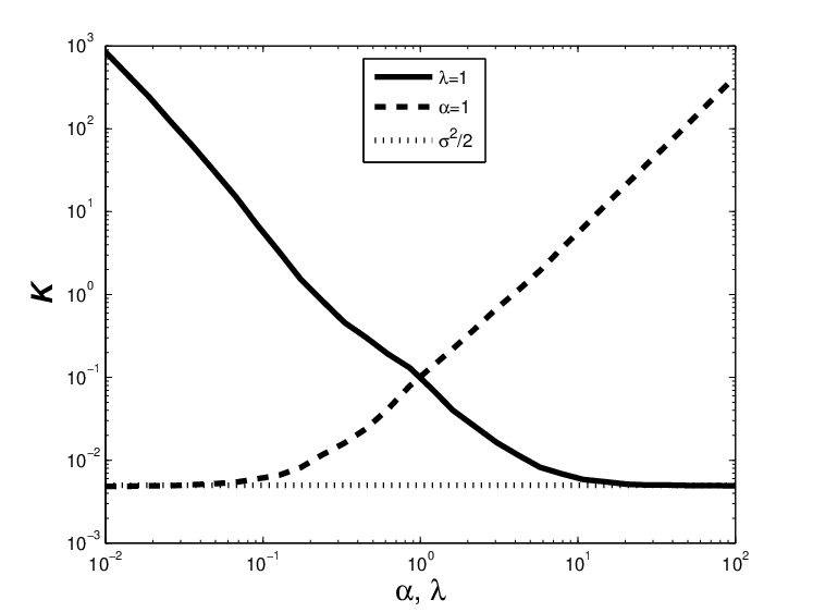
In this subesection we investigate the dependence of ${\mathcal{K}}$ on $\alpha$ and $\lambda$ for $\sigma=0.1,\,\tau=\delta=1.0$ . In the limit as either $\alpha\rightarrow\infty$ or $\lambda\rightarrow 0$ the OU processes converges to $0$ . It is expected, therefore, that in either of these two limits the solution of the Stokes equation converges to the solution of

\tau\ddot{x}=-\dot{x}+\sigma\xi(t),

(54)

and, consequently, in this limit the effective diffusivity is simply the molecular diffusion coefficient. This result can be derived using techniques from e.g. (Chapter 9 in [14]). On the other hand, when either $\alpha\rightarrow 0$ or $\lambda\rightarrow\infty$ , the OU process dominates the behavior of solutions to the Stokes equation and, consequently, the effective diffusivity is controlled by the OU process. The above intuition is supported by the numerical experiments presented in Figure 5. In particular, the effective diffusivity converges to $\frac{\sigma^{2}}{2}$ when either $\alpha$ becomes large or $\lambda$ becomes small, and becomes unbounded in the opposite limits.

5.4 The effect of $\delta$ on the diffusivity

In this section we study the effect of $\delta$ in the effective diffusivity of the colored noise problem. Our results are plotted in Figure 6. The values of $\alpha,\lambda$ are set equal to 1, while $\tau=1.3895$ and $\sigma=0.3162$ .

We expect that as $\delta\rightarrow 0$ the colored noise problem should approach the white noise problem. This is what we see in Figure 6, since when $\delta$ is of $\mathcal{O}(1)$ the value of the effective diffusivity for the colored noise problem is almost the same as the white noise one. The rate at which the effective diffusivity for the colored noise problem converge to the one for the white noise problem depends on the values of $\tau$ , $\sigma$ . Indeed, as we have already seen in subsection 5.1 for small values of $\tau$ and $\sigma$ there is a significant difference between the values for the two diffusivities when $\delta=\mathcal{O}(1)$ .

6 Conclusions

The problem of homogenization for inertial particles moving in a time dependent random velocity field was studied in this paper. It was shown, by means of formal multiscale expansions as well as rigorous mathematical analysis, that the long-time, large-scale behavior of the particles is governed by an effective Brownian motion. The covariance of the limiting Brownian motion can be expressed in terms of the solution of an appropriate Poisson equation.

The combined homogenization/rapid decorrelation in time for the velocity field limit was also studied. It was shown that the two limits commute.

Our theoretical findings were augmented by numerical experiments in which the dependence of the effective diffusivity on the various parameters of the problem was investigated. Furthermore, various limits of physical interest–such as $\sigma\rightarrow 0,\,\tau\rightarrow 0$ etc.–where studied. The results of our numerical experiments suggest that the effective diffusivity depends on the various parameters of the problem in a very complicated, highly nontrivial way.

There are still many questions that remain open. We list some of them.

•

Rigorous study of the dependence of the effective diffusivity on the various parameters of the problem. This problem has been studied quite extensively in the context of passive tracers. Apart for this being an interesting problem for the point of view of the physics of the problem, it also leads to some very interesting issues related to the spectral theory of degenerate, nonsymmetric second order elliptic operators.
•

Numerical experiments for more complicated flows. It is expected that the amount of enhancement of the diffusivity will depend sensitively on the detailed properties of the incompressible, time dependent flow.
•

Proof of a homogenization theorem for infinite dimensional OU processes, i.e. for the model (2). In this setting, questions such as the dependence of the effective diffusivity on the energy spectrum and the regularity of the flow can be addressed.

Appendix A Proof of the Homogenization Theorem

Let $x(t):{\mathbb{R}}^{+}\mapsto{\mathbb{R}}^{d}$ be the solution to the SDE

\tau\ddot{x}(t)=u(x(t),t)-\dot{x}(t)+\sigma\dot{\beta}_{1}(t),

(55)

where $\tau,\,\sigma>0$ , $\beta_{1}(t)$ is a standard Brownian motion on $\mathbb{R}^{d}.$ Furthermore the field $v(x,t):{\mathbb{R}}^{d}\times{\mathbb{R}}^{+}\mapsto{\mathbb{R}}^{d}$ is given by

u(x,t)=F(x)\mu(t).

Here, for each fixed $x$ , $F(x)\in{\mathbb{R}}^{d\times n}$ and, furthermore, $F(x)$ is smooth and period $1$ as a function of $x$ . Also $\mu(t):{\mathbb{R}}^{+}\mapsto{\mathbb{R}}^{n}$ is the solution of

\dot{\mu}(t)=-\delta^{-1}A\mu(t)+\delta^{-1}\sqrt{\Lambda}\dot{\beta}_{2}(t).

(56)

where $\beta_{2}(t)$ is a standard Brownian motion on ${\mathbb{R}}^{n}$ and $A,\,\Lambda$ are $n\times n$ positive definite matrices. Our goal is to prove that the rescaled process

x^{\epsilon}(t):=\epsilon x\left(\frac{t}{\epsilon^{2}}\right)

(57)

converges weakly to a Brownian motion with variance given by (23). We rewrite (55), (56) as a system of first order SDEs


$\displaystyle\dot{x}$	$\displaystyle=$	$\displaystyle\frac{1}{\sqrt{\tau}}y,$	(58a)
$\displaystyle\dot{y}$	$\displaystyle=$	$\displaystyle\frac{1}{\sqrt{\tau}}F(x)\mu-\frac{1}{\tau}y+\frac{\sigma}{\sqrt{\tau}}\dot{\beta_{1}},$	(58b)
$\displaystyle\dot{\mu}$	$\displaystyle=$	$\displaystyle-\frac{A}{\delta}\mu\ +\frac{\sqrt{\Lambda}}{\delta}\dot{\beta_{2}}.$	(58c)

This is a Markov process for $(x(t),y(t),\mu(t))$ on $\mathbb{R}^{d}\times\mathbb{R}^{d}\times\mathbb{R}^{n}$ . We let $z(t)$ denote the function $x(t)/\mathbb{Z}^{d}$ so that $z(t)\in\mathbb{T}^{d}=\mathbb{R}^{d}/\mathbb{Z}^{d}$ . Since $F$ is $1$ -periodic we may view $(z(t),y(t),\mu(t))$ as a Markov process on $\mathbb{T}^{d}\times\mathbb{R}^{d}\times\mathbb{R}^{n}$ .

Theorem A.1.

Let $\{x(t),\,y(t),\,\mu(t)\}$ be the Markov process defined through the solution of (58), where $A=I$ and $\Lambda=\lambda I,\,\lambda>0$ , $\sigma>0$ and assume that the process $\{z(t),y(t),\eta(t)\}$ is stationary. Assume that the vector field $F(x)\mu$ has zero expectation with respect to the invariant measure $\rho(z,y,\mu)dzdyd\mu$ of the Markov process $\{z(t),y(t),\mu(t)\}.$ Then the rescaled process $x^{\epsilon}(t)$ converges weakly to a Brownian motion with covariance matrix $2sym({\cal K})$ where

{\mathcal{K}}=\int_{{\mathbb{T}}^{d}\times{\mathbb{R}}^{d}\times{\mathbb{R}}^{n}}\left(-\mathcal{L}_{0}\Phi\right)\otimes\Phi\rho(z,y,\mu)dzdyd\mu.

(59)

Here $\Phi(z,y,\mu)\in L^{2}({\mathbb{T}}^{d}\times{\mathbb{R}}^{d}\times{\mathbb{R}}^{n},\rho(z,y,\mu)dzdyd\mu;{\mathbb{R}}^{d})$ is the unique–up to additive constants–solution of the Poisson equation

-\mathcal{L}_{0}\Phi=\frac{1}{\sqrt{\tau}}y.

(60)

Remark A.1.

The assumptions on $A$ and $\Lambda$ are made merely for notational simplicity. It is straightforward to extend the proof presented below to the case where $A,\,\Lambda$ are not diagonal matrices, provided that they are positive definite.

Remark A.2.

In the case where the centering condition (16), or equivalently (17), is not satisfied, then to leading order the particles move ballistically with an effective velocity $V=\langle F(z)\mu\rangle_{\rho}$ . A central limit theorem of the form of Theorem A.1 provides us with information on the fluctuations around the mean deterministic motion. See also Remark 3.2.

Remark A.3.

It is not necessary to assume that the process is started in its stationary distribution as it will approach this distribution exponentially fast. Indeed, as we prove in Proposition A.1 below, the fast process is geometrically ergodic. This implies that for every function $\psi:{\mathbb{T}}^{d}\times{\mathbb{R}}^{d}\times{\mathbb{R}}^{n}\mapsto\mathbb{R}$ which does not grow too fast at infinity there exist constants $C,\,\delta$ such that

\left|{\mathbb{E}}\left(\psi(z(t),y(t),\mu(t))\right)-\int_{{\mathbb{T}}^{d}\times{\mathbb{R}}^{d}\times{\mathbb{R}}^{n}}\psi(z,y,\mu)\rho(dzdyd\mu)\right|\leq Ce^{-\delta t},

(61)

where ${\mathbb{E}}$ denotes expectation with respect to the law of the process $\{z(t),\,y(t),\,\eta(t)\}$ and $\rho(z,y,\mu)dzdyd\mu$ the unique invariant measure. We make the stationarity assumption to avoid some technical difficulties.

As is usually the case with theorems of the form (A.1),e.g. [3, 25, 16, 18], the proof (A.1) is based on the cental limit theorem for additive functionals of Markov processes: we apply the Itô formula to the solution of the Poisson equation (20) to decompose the rescaled process (3) into a martingale part and a remainder; we then employ the martingale central limit theorem [9, Ch. 7] to prove a central limit theorem for the martingale part and we show that the remainder becomes negligible in the limit as $\epsilon\rightarrow 0$ . In order to obtain these two results we need to show that the fast process is ergodic and that the solution of the Poisson equation (20) exists and is unique in an appropriate class of functions, and that it satisfies certain a priori estimates. In order to prove that the fast process is ergodic in a sufficiently strong sense we use results from the ergodic theory of hypoelliptic diffusions [20]. In order to obtain the necessary estimates on the solution of the Poisson equation (20) we use results on the spectral theory of hypoelliptic operators [5, 6, 7, 8, 13]. Our overall approach is similar to the one developed in [12].

For the proof of the homogenization we will need the following three technical results which we prove in Appendix B.

Proposition A.1.

Let $\mathcal{L}_{0}$ be the operator defined in (13) and assume that $F(x)\in C^{\infty}({\mathbb{T}}^{d};{\mathbb{R}}^{n})$ and $\sigma>0$ . Then the process $\{z(t),\,y(t),\,\mu(t)\}$ generated by $\mathcal{L}_{0}$ is geometrically ergodic.

Proposition A.2.

Assume that $A=I,\,\Lambda=\lambda I,\,\lambda>0$ and $\sigma>0.$ Also let $\rho(z,y,\mu)$ be the invariant measure of the process generated by $\mathcal{L}_{0}$ . Then, for every $\alpha\in(0,2\sigma^{-2})$ and $\beta\in(0,2\lambda^{-1})$ there exists a function $g(z,y,\mu)\in{\mathcal{S}}$ (the Schwartz space of smooth functions with fast decay at infinity) such that

\rho(z,y,\mu)=e^{-\frac{\alpha}{2}\|y\|^{2}-\frac{\beta}{2}\|\mu\|^{2}}g(z,y,\mu).

(62)

Proposition A.3.

Let $h\in C^{\infty}({\mathbb{T}}^{d}\times{\mathbb{R}}^{d}\times{\mathbb{R}}^{n})$ with $D_{z,y,\mu}^{\alpha}h\in L^{2}({\mathbb{T}}^{d}\times{\mathbb{R}}^{d}\times{\mathbb{R}}^{n};e^{-\epsilon\|y\|^{2}-\epsilon\|\mu\|^{2}}dzdyd\mu)$ for every multiindex $\alpha$ and every $\epsilon>0$ . Assume further that $\int h(z,y,\eta)\,\rho(dz\,dy\,d\mu)=0$ , where $\rho$ is the invariant measure of the process $\{z(t),\ y(t),\ \mu(t)\}$ . Then there exists a solution $f$ of the equation

-\mathcal{L}_{0}f=h.

(63)

Moreover, for every $\alpha,\,\beta>0$ , the function $f$ satisfies

f(z,y,\mu)=e^{{\alpha\over 2}\|y\|^{2}+{\beta\over 2}\|\eta\|^{2}}\tilde{f}(z,y,\mu)\;,\qquad\tilde{f}\in{\mathcal{S}}\;.

(64)

Furthermore, for every $\alpha\in(0,2\sigma^{-2}),\,\beta\in(0,2\lambda^{-1})$ , $f$ is unique (up to an additive constant) in $L^{2}({\mathbb{T}}^{d}\times{\mathbb{R}}^{d}\times{\mathbb{R}}^{n},e^{-\alpha\|y\|^{2}-\beta\|\mu\|^{2}}dzdyd\mu)$ .

Proof of Theorem A.1. We have already shown that the centering assumption on the velocity field, equation (16), is equivalent to $\langle y\rangle_{\rho}=0$ . Moreover, $y$ clearly satisfies the smoothness and fast decay assumptions of Proposition A.3. Proposition A.3 applies to each component of equation (60) and we can conclude that there exists a unique smooth vector valued function $\Phi$ which solves the cell problem and whose components satisfy estimate (64).

We apply now Itô formula to $\Phi(x(t),y(t),\mu(t))$ with $(x,y,\mu)$ solving (66) and use the fact that $-\mathcal{L}_{0}\Phi=\frac{1}{\tau}y$ to obtain

$\displaystyle x^{\epsilon}(t)$	$\displaystyle=$	$\displaystyle\epsilon x(t/\epsilon^{2})$
	$\displaystyle=$	$\displaystyle\epsilon x(0)+\frac{\epsilon}{\sqrt{\tau}}\int_{0}^{t/\epsilon^{2}}y(s)ds$
	$\displaystyle=$	$\displaystyle\epsilon x(0)-\epsilon\left(\Phi(z(t/\epsilon^{2}),y(t/\epsilon^{2}),\mu(t/\epsilon^{2}))-\Phi(z(0),y(0),\mu(0))\right))$
		$\displaystyle+\epsilon\frac{\sigma}{\sqrt{\tau}}\int_{0}^{t/\epsilon^{2}}\nabla_{y}\Phi(y(s),z(s),\mu(s))d\beta_{1}(s)$
		$\displaystyle+\epsilon\frac{\sqrt{\lambda}}{\delta}\int_{0}^{t/\epsilon^{2}}\nabla_{\mu}\Phi(y(s),z(s),\mu(s))d\beta_{2}(s).$
	$\displaystyle=:$	$\displaystyle\epsilon x(0)+R^{\epsilon}_{t}+M^{\epsilon}_{t}+N^{\epsilon}_{t}.$

Clearly $\lim_{\epsilon\rightarrow 0}\epsilon^{2}{\mathbb{E}}|x(0)|^{2}=0$ . Furthermore, the stationarity assumption together with Propositions A.2 and A.3 imply that

\displaystyle{\mathbb{E}}|R^{\epsilon}_{t}|^{2}\leq C\epsilon^{2}\|\Phi(z,y,\mu)\|^{2}_{L^{2}_{\rho}}\leq C\epsilon^{2}.

(65)

Consider now the martingales $M^{\epsilon}_{t}$ and $N^{\epsilon}_{t}$ . According to the martingale central limit theorem [9, Thm. 7.1.4], in order to prove convergence of a martingale to a Brownian motion, it is enough to prove convergence of its quadratic variation in $L^{1}$ to $\sigma^{2}\,t$ ; $\sigma^{2}$ is the variance of the limiting Brownian motion. This now follows from propositions A.2 and A.3, together with the ergodic theorem for additive functionals of ergodic Markov processes [32]. In particular, using $\langle\cdot\rangle_{t}$ to denote the quadratic variation of a martingale, we have that

	$\displaystyle\langle M^{\epsilon}\rangle_{t}$	$\displaystyle=$	$\displaystyle\epsilon^{2}\frac{\sigma^{2}}{\tau}\int^{t/\epsilon^{2}}_{0}\nabla_{y}\Phi(x(s),y(s),\mu(s))\otimes\nabla_{y}\Phi(x(s),y(s),\mu(s))\,ds$
		$\displaystyle\rightarrow$	$\displaystyle\frac{\sigma^{2}}{\tau}\left\langle\nabla_{y}\Phi(x,y,\mu)\otimes\nabla_{y}\Phi(x,y,\mu)\right\rangle_{\rho}t\quad\mbox{in}\;\;L^{1}.$

Similarly

\displaystyle\langle N^{\epsilon}\rangle_{t}\rightarrow\frac{\lambda}{\delta^{2}}\left\langle\nabla_{\mu}\Phi(x,y,\mu)\otimes\nabla_{\mu}\Phi(x,y,\mu)\right\rangle_{\rho}t\quad\mbox{in}\;\;L^{1}.

We combine the above with equation (26) and use the fact that $\eta=\sqrt{\delta}\mu$ and that $A,\,\Lambda$ are diagonal matrices to conclude the proof of the theorem. ∎

Remark A.4.

With a bit of extra work one can also obtain estimates on the rate of convergence to the limiting Brownian motion in the Wasserstein metric, as was done in [12] for the case of a time independent velocity field. To accomplish this we need to obtain appropriate pathwise estimates on the rescaled particle velocity $y(t/\epsilon^{2})$ and the Ornstein–Uhlenbeck process $\mu(t/\epsilon^{2})$ . We also need to introduce an additional Poisson equation of the type (63) and to apply the Itô formula to its solution. The Poisson equation of type (63) plays the role of a higher order cell problem from the theory of homogenization; see ,e.g., [4] for the proof of an error estimate using higher order cell problems in the PDE setting. The argument used in [12, Thm. 2.1] is essentially a pathwise version of the PDE argument. We leave the details of this quantative error bound to the interested reader.

Appendix B Proof of Propositions A.1– A.3

In this section we prove that the operator $\mathcal{L}_{0}$ generates a geometrically ergodic Markov process. This means that there exists a unique invariant measure $\rho(dzdyd\mu)$ of the process which has a smooth density $\rho(z,y,\mu)$ with respect to Lebesgue measure on ${\mathbb{T}}^{d}\times{\mathbb{R}}^{d}\times{\mathbb{R}}^{n}$ ; and that, furthermore, estimate (61) holds. In addition, we prove some regularity properties of the invariant density and existence and uniqueness of solutions together with a priori estimates for the Poisson equation (20). The proof of Proposition A.1 follows the lines of [20]. The proof of Propositions A.2 and A.3 is based on results from [12].

The proof of this Proposition A.1 is based upon three lemmas. In the first lemma we show that the transition probability $P_{t}$ has a smooth density $\rho_{t}$ with respect to Lebesgue. In the second we show that $\rho_{t}$ is everywhere positive. In the third we show that there exists a Lyapunov function. These three lemmas imply that the fast process is geometrically ergodic [20, Cor. 2.8].

Lemma B.1.

Assume that $F(z)\in C^{\infty}({\mathbb{T}}^{d};{\mathbb{R}}^{n})$ . Then the Markov process generated by $\mathcal{L}_{0}$ has a smooth transition probability density $\rho_{t}$ .

Remark B.1.

The density $\rho_{t}$ is the solution of the evolution Fokker–Planck equation

\frac{\partial\rho_{t}}{\partial t}=\mathcal{L}_{0}^{*}\rho_{t}.

Proof.

This follows from Hormander’s theorem [33, Thm. 38.15]. The Markov process $\{z(t),\,y(t),\,\mu(t)\}$ generated by $\mathcal{L}_{0}$ solves the SDE


$\displaystyle dz$	$\displaystyle=$	$\displaystyle y\,dt,$	(66a)
$\displaystyle dy$	$\displaystyle=$	$\displaystyle\frac{1}{\tau}F(z)\mu\,dt-\frac{1}{\tau}y\,dt+\frac{\sigma}{\tau}\,dW_{1},$	(66b)
$\displaystyle d\mu$	$\displaystyle=$	$\displaystyle-A\mu\,dt+\sqrt{\Lambda}\,dW_{2},$	(66c)

with the understanding that $z\in\mathbb{T}^{d},y\in\mathbb{R}^{d}$ and $\mu\in\mathbb{R}^{n}$ . The Jacobian of the drift for this system is:

J=\left(\begin{array}[]{c|c|c}O_{d\times d}&I_{d\times d}&O_{d\times n}\\ \hline\cr\frac{1}{\tau}DF_{d\times d}&-\frac{1}{\tau}I_{d\times d}&\frac{1}{\tau}F_{d\times n}\\ \hline\cr O_{n\times d}&O_{n\times d}&-A_{n\times n}\end{array}\right)

where

(DF)_{k,l}=\frac{\partial}{\partial x_{l}}\sum_{i=1}^{m}F_{ki}(x)\mu_{i}.

In order to prove that our system is hypo-elliptic we need to span $\mathbb{R}^{2d+n}$ through the noise vectors and their Lie commutators with the drift. We are going to study two cases. The first is when $\sigma\neq 0$ . In this case the noise provides the vectors:

e^{(i)}_{j}=\delta_{ij},\ \ \ i=d+1,\ldots 2d+n.\ \text{and}\ j=1,\ldots,2d+n.

thus we are missing $d$ vectors in order to span $\mathbb{R}^{2d+n}$ . We can see that we can obtain the missing vectors $e^{(i)}_{j},\ i=1,\ldots d$ in the following way:

Je^{(i)}=e^{(i-d)}-\frac{1}{\tau}e^{(i)},\ \ i=d+1,\ldots,2d

thus we obtained the vectors $e^{(i)},\ i=1\ldots 2d+n$ that span $\mathbb{R}^{2d+n}\qed.$

Remark B.2.

We briefly remark on the case where $\sigma=0$ . In this case since there is no noise in the equation describing the motion of $x$ and $y$ we need to span $\mathbb{R}^{2d+n}$ having the following vectors:

e^{(i)}_{j}=\delta_{ij},\ \ \ i=2d+1,\ldots 2d+n.\ \text{and}\ j=1,\ldots,2d+n.

We notice that:

(Je^{(i)})_{j}=\begin{cases}0&\text{if $j=1,\ldots,d$}\\ F_{(j-2d)(i-2d)}&\text{if $j=d+1,\ldots,2d$}\\ A_{(j-2d)(i-2d)}\text{if $j=2d+1,\ldots,j=2d+n$}\end{cases}

So the only way not to obtain the vectors $e^{(i)},\ i=d+1,\ldots,2d$ is if the following equation holds:

F_{lk}(z)=0,\ \forall l\in\{1,\ldots n\}\ \text{and}\ k\in\{1,\ldots k\}

If this equation does not hold we can obtain the rest of the vectors in the exact same way as we did in the case where $\sigma\neq 0.$

Lemma B.2.

For all $Z:=(z,y,\mu)\in\mathbb{T}^{d}\times\mathbb{R}^{d}\times\mathbb{R}^{n},\,t>0$ and open $\mathcal{O}\subset\mathbb{T}^{d}\times\mathbb{R}^{d}\times\mathbb{R}^{n}$ , the transition kernel corresponding to the Markov process $\{z(t),\,x(t),\mu(t)\}$ defined in (66) satisfies $P_{t}(z,\mathcal{O})>0$ .

Proof.

The proof of this result is based on a controllability argument [38, 7, 20]. We start by writing (66) compactly in the form

dZ=Y(Z)\,dt+\Sigma dW

(67)

with $Y(Z)=[y,\,\frac{1}{\tau}F(z)\mu-\frac{1}{\tau}y,-A\mu]^{T}$ , $W(t)=[W_{1}(t),\,W_{2}(t)]^{T}$ and

\displaystyle\Sigma=\left(\begin{array}[]{c c}O_{d\times d}&O_{d\times n}\\ \frac{\sigma}{\tau}I_{d\times d}&O_{d\times n}\\ O_{d\times d}&\sqrt{\lambda}\end{array}\right).

The control problem associated with (66) is

\frac{dR}{dt}=Y(R)+\Sigma\frac{dU}{dt}.

(69)

For any $t>0$ , any $a\in\mathbb{T}^{d}\times\mathbb{R}^{d}\times\mathbb{R}^{n}$ , and any $a^{+}\in\mathbb{T}^{d}\times\mathbb{R}^{d}\times\mathbb{R}^{n}$ we can find smooth $U\in C^{1}([0,t],\mathbb{R}^{d+n})$ such that (69) is satisfied and $X(0)=a,X(t)=a^{+}$ . To see this set $R=((X^{T},\frac{dX}{dt}^{T},M^{T})^{T})$ . The equation for $M$ is

\frac{dM}{dt}=-AM+\sqrt{\Lambda}\frac{dU_{2}}{dt}.

We consider this equation separately since it does not involve any of the other state variables. Choose $M$ to be a $C^{\infty}$ path such that, for the given $t>0$ ,

M(0)=a_{3},M(t)=a^{+}_{3}

(70)

where with $a_{3},a_{3}^{+}$ we denote the last $n$ components of the vectors $a,a^{+}$ . Since $\sqrt{\Lambda}$ is positive definite is invertible and $\frac{dU_{2}}{dt}$ is defined by substitution and will be as smooth as $M$ and $(\sqrt{\Lambda})^{-1}$ hence $C^{\infty}$ . Also $U(0)$ can be taken as 0. The equation for $(X^{T},\frac{dX}{dt}^{T})^{T})$ is

\tau\frac{d^{2}X}{dt^{2}}+\frac{dX}{dt}+F(X)M=\sigma\frac{dU_{1}}{dt}.

where $U_{2}$ is chosen that $M$ satisfies (69) . Now let X be a $C^{\infty}$ path such that, for that given t

\left(\begin{array}[]{c}X(0)\\ \frac{dX}{dt}(0)\end{array}\right)=a_{1}\hskip 28.45274pt\left(\begin{array}[]{c}X(t)\\ \frac{dX}{dt}(t)\end{array}\right)=a^{+}_{1}

where with $a_{1},a^{+}_{1}$ we denote the first $2d$ elements of the vectors $a,a^{+}$ respectively. Since $\sigma$ is everywhere invertible, $\frac{dU_{1}}{dt}$ is defined by substitution and will be as smooth as $F(X)M$ and $\sigma^{-1}$ – hence $C^{\infty}$ . Also $U_{1}(0)$ can be taken as 0.

Now note that the event

\sup_{0\leq s\leq t}||W_{2}(s)-U_{2}(s)||\leq\epsilon

occurs with positive probability since the Wiener measure of any tube is positive. So the Brownian motion $\beta_{2}$ controls the $\eta$ component of equation (66). Again note that the event

\sup_{0\leq s\leq t}||W_{1}(s)-U_{1}(s)||\leq\epsilon

occurs with positive probability since the Wiener measure of any such tube is positive. Combining now these two results is possible to deduce the required open set irreducibility. ∎

Lemma B.3.

Let $\lambda_{1}$ be the smallest eigenvalue of $A$ and $F=\sup_{x\in\mathbb{T}^{d}}||F(x)||$ . Then there exists a constant $\beta>0$ such that the function $V(x,y,\mu)=1+\frac{2\tau}{2}||y||^{2}+\frac{\tau^{2}F^{2}+1}{2\lambda_{1}}||\mu||^{2}$ satisfies

\mathcal{L}_{0}\bigl(V(x,y,\mu)\bigr)\leq-V(x,y,\mu)+\beta

Proof.

We have that $V(x,y,\mu)$ maps the state space onto $[1,\infty)$ and that $\lim_{||y||,||\mu||\rightarrow\infty}=+\infty$ . Moreover we have

$\displaystyle\mathcal{L}_{0}\bigl(V(x,y,\mu)\bigr)$	$\displaystyle=$	$\displaystyle F(x)\mu\cdot 2\tau y-2\|\|y\|\|^{2}+\frac{\sigma^{2}}{2}d-\frac{\tau^{2}F^{2}+1}{\lambda_{1}}A\mu\cdot\mu+\frac{trace(\Lambda)}{2}$
	$\displaystyle\leq$	$\displaystyle\tau^{2}F^{2}\|\|\mu\|\|^{2}+\frac{4\tau^{2}}{4\tau^{2}}\|\|y\|\|^{2}-2\|\|y\|\|^{2}-\frac{(\tau^{2}F^{2}+1)\lambda_{1}}{\lambda_{1}}\|\|\mu\|\|^{2}$
	$\displaystyle+$	$\displaystyle\frac{trace(\Lambda)}{2}+\frac{\sigma^{2}}{2}d$
	$\displaystyle\leq$	$\displaystyle-V(x,y,\mu)+\beta,$

with $\beta=\frac{\sigma^{2}d}{2}+\frac{trace(\Lambda)}{2}+1$ . ∎

Proof of Proposition A.1. It follows from the above three lemmas and [20, Cor. 2.8]. ∎

Using results from [8, 5] we can also derive some regularity estimates for the invariant density. In addition, we can show that the operator $\mathcal{L}_{0}^{*}$ , the formal $L^{2}$ –adjoint of $\mathcal{L}_{0}$ , has compact resolvent and, hence, Fredholm theory applies.

Proof of Proposition A.2 The proof of this result is similar to the proof of [12, Thm. 3.1], which in turn follows the lines of [8, 5]. Denote by $\phi_{t}$ the (random) flow generated by the solutions to (66) and by ${\mathcal{P}}_{t}$ the semigroup defined on finite measures by

\left({\mathcal{P}}_{t}\mu\right)(A)={\mathbb{E}}\left(\mu\circ\phi_{t}^{-1}\right)(A)\;.

(71)

By Lemma B.1 ${\mathcal{P}}_{t}$ maps every measure into a measure with a smooth density with respect to the Lebesgue measure. It can therefore be restricted to a positivity preserving contraction semigroup on $L^{1}({\mathbb{T}}^{d}\times{\mathbb{R}}^{d}\times{\mathbb{R}}^{n},dz\,dy\,d\mu)$ . The generator ${\mathcal{L}}_{0}^{*}$ of ${\mathcal{P}}_{t}$ is the formal $L^{2}$ –adjoint of ${\mathcal{L}}_{0}$ .

We now define an operator $K$ on $L^{2}({\mathbb{T}}^{d}\times{\mathbb{R}}^{d}\times{\mathbb{R}}^{n},dz\,dy\,d\mu)$ by closing the operator defined on ${\mathcal{C}}_{0}^{\infty}$ by

$\displaystyle K$	$\displaystyle=$	$\displaystyle-e^{\frac{\alpha}{2}\\|y\\|^{2}+\frac{\beta}{2}\\|\mu\\|^{2}}{\mathcal{L}}^{*}e^{-\frac{\alpha}{2}\\|y\\|^{2}-\frac{\beta}{2}\\|\mu\\|^{2}}$
	$\displaystyle=$	$\displaystyle-{\sigma^{2}\over 2}\Delta_{y}-{\lambda\over 2}\Delta_{\mu}+\beta\left(1-\frac{\lambda\beta}{2}\right)\\|\mu\\|^{2}+\alpha\left(1-\frac{\sigma^{2}\alpha}{2}\right)\\|y\\|^{2}$
		$\displaystyle+(\sigma^{2}\alpha^{2}-1)\left(y\cdot\nabla_{y}+\frac{n}{2}\right)+(\lambda\beta-1)\left(\mu\cdot\nabla_{\mu}+\frac{d}{2}\right)$
	$\displaystyle-$	$\displaystyle\alpha y\cdot F(z,\mu)-\frac{n}{2}-\frac{d}{2}.$

Note at this point that $\alpha<2\sigma^{-2}$ and $\beta<2\lambda^{-1}$ is required to make the coefficients of $\|y\|^{2}$ and $\|\mu\|^{2}$ , respectively, strictly positive.

We can rewrite the above expression in Hörmander’s “sum of squares” form as

K=\sum_{i=1}^{2d+2n}X_{i}^{*}X_{i}+X_{0}\;,

(72)

with

$\displaystyle X_{i}$	$\displaystyle=$	$\displaystyle\frac{\sigma}{\sqrt{2}}\partial_{y_{i}}\quad\mbox{for $i=1\ldots d$,}$
$\displaystyle X_{i}$	$\displaystyle=$	$\displaystyle\sqrt{\frac{\lambda}{2}}\partial_{\mu_{i-d}}\quad\mbox{for $i=n+1\ldots(n+d)$}$
$\displaystyle X_{i}$	$\displaystyle=$	$\displaystyle\sqrt{\alpha\left((1-{\alpha\sigma^{2}\over 2}\right))}y_{i-n-d}\quad\mbox{for $i=(n+d+1)\ldots 2n+d$,}$
$\displaystyle X_{i}$	$\displaystyle=$	$\displaystyle\sqrt{\beta\left((1-{\lambda\beta\over 2}\right))}\mu_{i-2n-d}\quad\mbox{for $i=(2n+d+1)\ldots(2n+2d)$,}$
$\displaystyle X_{0}$	$\displaystyle=$	$\displaystyle(\sigma^{2}\alpha^{2}-1)\left(y\cdot\nabla_{y}+\frac{n}{2}\right)+(\lambda\beta-1)\left(\mu\cdot\nabla_{\mu}+\frac{d}{2}\right)-\alpha y\cdot F(z,\mu)-\frac{n}{2}-\frac{d}{2}.$

Since $F$ is $C^{\infty}$ on the torus, it can be checked that the assumptions of [5, Thm. 5.5] are satisfied with $\Lambda^{2}=1-\Delta_{z}-\Delta_{y}-\Delta_{\mu}+\|y\|^{2}+\|\mu\|^{2}$ . Combining this with [5, Lem. 5.6], we see that there exists $\alpha>0$ such that, for every $\gamma>0$ , there exists a positive constant $C$ such that

\|\Lambda^{\alpha+\gamma}f\|\leq C\left(\|\Lambda^{\gamma}Kf\|+\|\Lambda^{\gamma}f\|\right)\;,

(73)

holds for every $f$ in the Schwartz space. Clearly, the operator $\Lambda^{2}$ has compact resolvent. This, together with (73) with $\gamma=0$ and [5, Prop. 5.9] imply that $K$ has compact resolvent.

Notice now that

K^{*}=-e^{-\frac{\alpha}{2}\|y\|^{2}-\frac{\beta}{2}\|\mu\|^{2}}{\mathcal{L}}e^{\frac{\alpha}{2}\|y\|^{2}+\frac{\beta}{2}\|\mu\|^{2}}.

Thus, $e^{-\frac{\alpha}{2}\|y\|^{2}-\frac{\beta}{2}\|\mu\|^{2}}$ is the solution of the homogeneous equation

K^{*}e^{-\frac{\alpha}{2}\|y\|^{2}-\frac{\beta}{2}\|\mu\|^{2}}=0.

(74)

The compactness of the resolvent of $K$ implies that there exists a function $g$ such that

Kg=0.

Estimate (73), together with a simple approximation argument imply that $\|\Lambda^{\gamma}g\|<\infty$ for every $\gamma>0$ , and therefore $g$ belongs to the Schwartz space. Furthermore, an argument given for example in [8, Prop 3.6] shows that $g$ must be positive. Since one has furthermore

{\mathcal{L}}^{*}e^{-\frac{\alpha}{2}\|y\|^{2}-\frac{\beta}{2}\|\mu\|^{2}}g=0\;,

(75)

the invariant density $\rho$ satisfies estimate (62). ∎

The ergodicity of the fast process, together with the above proposition enable us to prove the following lemma.

Lemma B.4.

Let $\alpha\in(0,2\sigma^{-2}),\,\beta\in(0,2\lambda^{-1})$ and let $K$ be as in the proof of Proposition A.2. Then, the kernel of $K$ is one-dimensional.

Proof.

Let $\tilde{g}\in\ker K$ . Then, by the same arguments as above, $e^{-{\alpha\over 2}\|y\|^{2}-{\beta\over 2}\|\mu\|^{2}}\tilde{g}$ is the density of an invariant signed measure for ${\mathcal{P}}_{t}$ . The ergodicity of ${\mathcal{P}}_{t}$ immediately implies $\tilde{g}\propto g$ . ∎

Now we are ready to prove estimates on the solution of the Poisson equation (60).

Proof of Proposition A.3 By hypoellipticity, if there exists a distribution $f$ such that (63) holds, then $f$ is actually a $C^{\infty}$ function.

We start with the proof of existence. Fix $\alpha\in(0,2\sigma^{-2}),\,\beta\in(0,2\lambda^{-1})$ , consider the operator $K^{*}$ defined in (74), and define the function

u(z,y,\mu)=h(z,y,\eta)\,e^{-{\alpha\over 2}\|y\|^{2}-{\beta\over 2}\|\mu\|^{2}}\;.

It is clear that if there exists $\tilde{f}$ such that $K^{*}\tilde{f}=u$ , then $f=e^{{\alpha\over 2}\|y\|^{2}+{\beta\over 2}\|\mu\|^{2}}\tilde{f}$ is a solution to (63). Consider the operator $K^{*}K$ . By the considerations in the proof of Proposition A.2, $K^{*}K$ has compact resolvent. Furthermore, the kernel of $K^{*}K$ is equal to the kernel of $K$ , which in turn by Lemma B.4 is equal to the span of $g$ . Define ${\mathcal{H}}=\langle g\rangle_{\rho}^{\bot}$ and define $M$ to be the restriction of $K^{*}K$ to ${\mathcal{H}}$ . Since $K^{*}K$ has compact resolvent, it has a spectral gap and so $M$ is invertible. Furthermore, we have that $f\in{\mathcal{H}}$ , therefore $\tilde{f}=KM^{-1}u$ solves $K^{*}\tilde{f}=u$ and thus leads to a solution to (63).

Since $K^{*}$ satisfies a similar bound to (73) and since $\|\Lambda^{\gamma}u\|<\infty$ for every $\gamma>0$ , the bound (64) follows as in Proposition A.2. The uniqueness of $u$ in the class of functions under consideration follows immediately from Lemma B.4. ∎

Remark B.3.

Note that the solution $f$ of (63) may not be unique if we allow for functions that grow faster than $e^{\sigma^{-2}\|y\|^{2}+\lambda^{-1}\|\mu\|^{2}}$ .

References

[1] A. Bensoussan, J.L. Lions, and G. Papanicolaou. Asymptotic analysis of periodic structures. North-Holland, Amsterdam, 1978.
[2] R.A. Carmona and F. Cerou. Transport by incompressible random velocity fields: simulations & mathematical conjectures. In Stochastic partial differential equations: six perspectives, volume 64 of Math. Surveys Monogr., pages 153–181. Amer. Math. Soc., Providence, RI, 1999.
[3] R.A. Carmona and L. Xu. Homogenization theory for time-dependent two-dimensional incompressible gaussian flows. The Annals of Applied Probability, 7(1):265–279, 1997.
[4] D. Cioranescu and P. Donato. An Introduction to Homogenization. Oxford University Press, New York, 1999.
[5] J.-P. Eckmann and M. Hairer. Non-equilibrium statistical mechanics of strongly anharmonic chains of oscillators. Comm. Math. Phys., 212(1):105–164, 2000.
[6] J.-P. Eckmann and M. Hairer. Spectral properties of hypoelliptic operators. Comm. Math. Phys., 235(2):233–253, 2003.
[7] J-P. Eckmann, C-A. Pillet, and L. Rey-Bellet. Entropy production in nonlinear, thermally driven Hamiltonian systems. J. Statist. Phys., 95(1-2):305–331, 1999.
[8] J.-P. Eckmann, C.-A. Pillet, and L. Rey-Bellet. Non-equilibrium statistical mechanics of anharmonic chains coupled to two heat baths at different temperatures. Comm. Math. Phys., 201(3):657–697, 1999.
[9] S.N. Ethier and T.G. Kurtz. Markov processes. Wiley Series in Probability and Mathematical Statistics: Probability and Mathematical Statistics. John Wiley & Sons Inc., New York, 1986.
[10] G. Falkovich, A. Fouxon, and M.G. Stepanov. Acceleration of rain initiation by cloud turbulence. Nature, 419:151–154, 2002.
[11] G. Falkovich, K. Gawȩdzki, and M. Vergassola. Particles and fields in fluid turbulence. Rev. Modern Phys., 73(4):913–975, 2001.
[12] M. Hairer and G.A. Pavliotis. Periodic homogenization for hypoelliptic diffusions. J. Statist. Phys., 117(1-2):261–279, 2004.
[13] B. Helffer and F. Nier. Hypoelliptic estimates and spectral theory for Fokker-Planck operators and Witten Laplacians, volume 1862 of Lecture Notes in Mathematics. Springer-Verlag, Berlin, 2005.
[14] W. Horsthemke and R. Lefever. Noise-induced transitions, volume 15 of Springer Series in Synergetics. Springer-Verlag, Berlin, 1984. Theory and applications in physics, chemistry, and biology.
[15] P.E. Kloeden and E. Platen. Numerical solution of stochastic differential equations, volume 23 of Applications of Mathematics (New York). Springer-Verlag, Berlin, 1992.
[16] Tomasz Komorowski and Stefano Olla. On homogenization of time-dependent random flows. Probab. Theory Related Fields, 121(1):98–116, 2001.
[17] R. Kupferman, G. A. Pavliotis, and A. M. Stuart. Itô versus Stratonovich white-noise limits for systems with inertia and colored multiplicative noise. Phys. Rev. E (3), 70(3):036120, 9, 2004.
[18] C. Landim, S. Olla, and H. T. Yau. Convection-diffusion equation with space-time ergodic random flow. Probab. Theory Related Fields, 112(2):203–220, 1998.
[19] A.J. Majda and P.R. Kramer. Simplified models for turbulent diffusion: Theory, numerical modelling and physical phenomena. Physics Reports, 314:237–574, 1999.
[20] J.C. Mattingly and A. M. Stuart. Geometric ergodicity of some hypo-elliptic diffusions for particle motions. Markov Processes and Related Fields, 8(2):199–214, 2002.
[21] M.R. Maxey. Gravitational settling of aerosol particles in homogeneous turbulence and random flow fields. J. Fluid Mech., 174:441–465, 1987.
[22] M.R. Maxey. The motion of small spherical particles in a cellular flow field. Phys. Fluids, 30(7):1915–1928, 1987.
[23] M.R. Maxey. On the advection of spherical and nonspherical particles in a nonuniform flow. Philos. Trans. Roy. Soc. London Ser. A, 333(1631):289–307, 1990.
[24] M.R. Maxey and J.J. Riley. Equation of motion for a small rigid sphere in a nonuniform flow. Phys. Fluids, 26:883–889, 1983.
[25] G. C. Papanicolaou, D.W. Stroock, and S. R. S. Varadhan. Martingale approach to some limit theorems. In Papers from the Duke Turbulence Conference (Duke Univ., Durham, N.C., 1976), Paper No. 6, pages ii+120 pp. Duke Univ. Math. Ser., Vol. III. Duke Univ., Durham, N.C., 1977.
[26] G. A. Pavliotis and A. M. Stuart. White noise limits for inertial particles in a random field. Multiscale Model. Simul., 1(4):527–533 (electronic), 2003.
[27] G. A. Pavliotis and A. M. Stuart. Analysis of white noise limits for stochastic systems with two fast relaxation times. Multiscale Model. Simul., 4(1):1–35 (electronic), 2005.
[28] G. A. Pavliotis and A. M. Stuart. Periodic homogenization for inertial particles. Phys. D, 204(3-4):161–187, 2005.
[29] G.A. Pavliotis. A multiscale approach to Brownian motors. Phys. Lett. A, 344:331–345, 2005.
[30] G.A. Pavliotis and A.M. Stuart. An introduction to Multiscale Methods. Lecture Notes, 2006.
[31] G.A. Pavliotis, A.M. Stuart, and L. Band. Monte Carlo studies of effective diffusivities for inertial particles. In Monte Carlo and quasi-Monte Carlo methods 2004, pages 431–441. Springer, Berlin, 2006.
[32] D. Revuz and M. Yor. Continuous martingales and Brownian motion, volume 293 of Grundlehren der Mathematischen Wissenschaften [Fundamental Principles of Mathematical Sciences]. Springer-Verlag, Berlin, third edition, 1999.
[33] L. C. G. Rogers and David Williams. Diffusions, Markov processes, and martingales. Vol. 2. Cambridge Mathematical Library. Cambridge University Press, Cambridge, 2000.
[34] J. Rubin, C. K. R. T. Jones, and M. Maxey. Settling and asymptotic motion of aerosol particles in a cellular flow field. J. Nonlinear Sci., 5(4):337–358, 1995.
[35] R. A. Shaw. Particle-turbulence interactions in atmosphere clouds. Annu. Rev. Fluid Mech., 35:183–227, 2003.
[36] H. Sigurgeirsson and A. M. Stuart. Inertial particles in a random field. Stoch. Dyn., 2(2):295–310, 2002.
[37] H. Sigurgeirsson and A. M. Stuart. A model for preferential concentration. Phys. Fluids, 14(12):4352–4361, 2002.
[38] D.W. Stroock and S.R.S. Varadhan. On the support of diffusion processes with applications to the strong maximum principle. In Proceedings of the Sixth Berkeley Symposium on Mathematical Statistics and Probability (Univ. California, Berkeley, Calif., 1970/1971), Vol. III: Probability theory, pages 333–359, Berkeley, Calif., 1972. Univ. California Press.
[39] L.P. Wang, M.R. Maxey, T.D. Burton, and D.E. Stock. Chaotic dynamics of particle dispersion in fluids. Phys. Fluids A, 4(8):1789–1804, 1992.

Homogenization for Inertial Particles in a Random Flow

Abstract

1 Introduction

2 The Model

3 Multiple Scales Expansion for Effective Diffusivities

3.1 Homogenization for the colored velocity field

3.1.1 Multiscale expansion

3.1.2 The homogenization result

Result 3.1.

3.1.3 Properties of the effective diffusivity

Result 3.2.

Remark 3.1.

Remark 3.2.

3.2 Homogenization: the white noise velocity field

3.2.1 The homogenization result

Result 3.3.

3.2.2 Properties of the effective diffusivity

Result 3.4.

Remark 3.3.

4 White Noise Limit for the Effective Diffusivity

Result 4.1.

4.1 Expansion for ϕα\phi^{\alpha}

4.2 Expansion for ρ\rho

4.3 Proof of Result 4.1

Remark 4.1.

5 Numerical Investigations

5.1 The effect of τ\tau on the diffusivity

5.2 The effect of σ\sigma on the diffusivity

5.3 The effect of α\alpha and λ\lambda on the effective diffusivity

5.4 The effect of δ\delta on the diffusivity

6 Conclusions

Appendix A Proof of the Homogenization Theorem

Theorem A.1.

Remark A.1.

Remark A.2.

Remark A.3.

Proposition A.1.

Proposition A.2.

Proposition A.3.

Remark A.4.

Appendix B Proof of Propositions A.1– A.3

Lemma B.1.

Remark B.1.

Proof.

Remark B.2.

Lemma B.2.

Proof.

Lemma B.3.

Proof.

Lemma B.4.

Proof.

Remark B.3.

References

4.1 Expansion for $\phi^{\alpha}$

4.2 Expansion for $\rho$

5.1 The effect of $\tau$ on the diffusivity

5.2 The effect of $\sigma$ on the diffusivity

5.3 The effect of $\alpha$ and $\lambda$ on the effective diffusivity

5.4 The effect of $\delta$ on the diffusivity