Waveguides with combined Dirichlet and Robin boundary conditions

Given an open interval $I\subseteq\mathbb{R}$ (bounded or unbounded), let $\Gamma\equiv(\Gamma^{1},\Gamma^{2}):I\to\mathbb{R}^{2}$ be a unit-speed $C^{2}$-smooth plane curve. We assume that $\Gamma$ is an embedding. The function $N:=(-\dot{\Gamma}^{2},\dot{\Gamma}^{1})$ defines a unit normal vector field along $\Gamma$ and the couple $(\dot{\Gamma},N)$ gives a distinguished Frenet frame (cf [23, Chap. 1]). The curvature of $\Gamma$ is defined through the Serret-Frenet formulae by $\kappa:=\det(\dot{\Gamma},\ddot{\Gamma})$; it is a continuous function of the arc-length parameter. We assume that $\kappa$ is bounded. It is worth noticing that the curve $\Gamma$ is fully determined (except for its position and orientation in the plane) by the curvature function $\kappa$ alone (cf [26, Sec. II.20]).

Let $a$ be a given positive number. We define the mapping

and make the hypotheses that

Then the image

has a geometrical meaning of an open non-self-intersecting strip, contained between the parallel curves

at the distance $a$ from $\Gamma$, and, if $\partial I$ is not empty, the straight lines $L_{-}:=\mathcal{L}\big(\{\inf I\}\times(-a,a)\big)$ and $L_{+}:=\mathcal{L}\big(\{\sup I\}\times(-a,a)\big)$. The geometry is set in such a way that $\kappa>0$ implies that the parallel curve $\Gamma_{+}$ is locally shorter than $\Gamma_{-}$, and vice versa. We refer to [12, App. A] for a sufficient condition ensuring the validity of the second hypothesis in (2).

Given a bounded continuous function $\tilde{\alpha}:\Gamma_{+}\to\mathbb{R}$, let $-\Delta_{\kappa,\alpha}$ denote the (non-negative) Laplacian on $L^{2}(\Omega)$, subject to uniform Dirichlet boundary conditions on the parallel curve $\Gamma_{-}$, uniform Neumann boundary conditions on $L_{-}\cup L_{+}$ (i.e. none if $\partial I$ is empty) and the Robin boundary conditions of the form

where $u\in D(-\Delta_{\kappa,\alpha})$. Hereafter we shall rather use $\alpha:=\tilde{\alpha}\big(\mathcal{L}(\cdot,a)\big)$, a function on $I$. Notice that the choice $\alpha=0$ corresponds to uniform Neumann boundary conditions on $\Gamma_{+}$ and $\alpha\to+\infty$ approaches uniform Dirichlet boundary conditions on $\Gamma_{+}$; for this reason, we shall sometimes use “$\alpha=+\infty$” to refer to the latter. The Laplacian $-\Delta_{\kappa,\alpha}$ is properly defined in Section 3 below by means of a quadratic-form approach.

If the curvature $\kappa$ is a constant function, then the image $\Omega$ can be identified with a segment of an annulus or a straight strip. We prove that, in certain situations, this constant geometry minimizes the spectrum of $-\Delta_{\kappa,\alpha}$, within all admissible functions $\kappa$ and $\alpha$ considered as parameters.

More precisely, let us denote by $\mathcal{D}(r)$ the open disc of radius $r>0$ and let $\mathcal{A}(r_{1},r_{2}):=\mathcal{D}(r_{2})\setminus\overline{\mathcal{D}(r_{1})}$ be an annulus of radii $r_{2}>r_{1}>0$. Abusing the notation for $\kappa$ and $\alpha$ slightly, we introduce a function $\lambda:(-a,a)\times\mathbb{R}\to\mathbb{R}$ by means of the following definition:

The most general result of the present paper reads as follows:

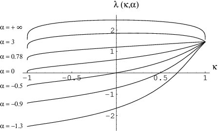
The lower bound $\lambda(\kappa,\alpha)$ as a function of curvature $\kappa$ for certain values of $\alpha$ is depicted in Figure 1. We prove the following properties which are important for (5):

Of course, $\nu(+\infty)=j_{0,1}^{2}/(2a)^{2}$, where $j_{0,1}$ denotes the first zero of the Bessel function $J_{0}$, and $\nu(0)=0$.

Theorem 1 is a natural continuation of efforts to estimate the spectral threshold in curved Dirichlet tubes [2, 14]. More specifically, in the recent article [14], Exner and the present authors establihed a lower bound of the type (5) for the case $\alpha=+\infty$, i.e. for pure Dirichlet strips (the results in that paper are more general in the sense that the tubes considered there were multi-dimensional and of arbitrary cross-section). Namely,

where $\lambda(\kappa,+\infty)$ is the spectral threshold of the Dirichlet Laplacian in $\mathcal{A}_{\kappa}$. It is also established in [14] that $\kappa\mapsto\lambda(\kappa,+\infty)$ is an even function, decreasing on $[0,1/a)$, reaching its maximum $\pi^{2}/(2a)^{2}$ for $\kappa=0$ (a straight strip) and approaching its infimum $\nu(+\infty)$ as $\kappa\to 1/a$ (a disc). The style and the main idea (i.e. the intermediate lower bound (14) below) of the present paper are similar to that of [14]. However, we have to use different techniques to establish the properties of $\lambda$ (Theorem 2), and consequently (5).

Theorem 1 is optimal in the sense that the lower bound (5) is achieved by a strip (along a curve of constant curvature). On the other hand, since the minimizer is bounded if the curvature is non-trivial, a better lower bound is expected to hold for unbounded strips. Indeed, in certain unbounded situations, we prove that the lower bound of Theorem 1 can be improved by a Hardy-type inequality.

Let us therefore consider the infinite case $I=\mathbb{R}$ in this subsection. Let $\alpha_{0}$ be a given real number. If $\kappa$ is equal to zero identically (i.e. $\Omega$ is a straight strip) and $\alpha$ is equal to $\alpha_{0}$ identically, it is easy to see that

Although the results below hold under more general conditions about vanishing of $\kappa$ and the difference $\alpha-\alpha_{0}$ at infinity (cf Section 7 below), for simplicity, we restrict ourselves to strips which are deformed only locally in the sense that $\kappa$ and $\alpha-\alpha_{0}$ have compact support. Under these hypotheses, it is easy to verify that the essential spectrum is preserved:

A harder problem is to decide whether this interval exhausts the spectrum of $-\Delta_{\kappa,\alpha}$, or whether there exists discrete eigenvalues below $\lambda(0,\alpha_{0})$.

On the one hand, Dittrich and Kříž [9] showed that the curvature which is negative in a suitable sense creates eigenvalues below the threshold $\lambda(0,0)$ in the uniform Dirichlet-Neumann case (i.e. in the case $\alpha=0$ identically). For instance, using, in analogy to [9], a modification of the “generalized eigenfunction” of $-\Delta_{0,\alpha_{0}}$ corresponding to $\lambda(0,\alpha_{0})$ as a test function, it is straightforward to extend a result of [9] to the case of uniform Robin boundary conditions:

On the other hand, Dittrich and Kříž [9] showed that the spectrum of $-\Delta_{\kappa,0}$ coincides with the interval (7) with $\alpha_{0}=0$ provided the curvature $\kappa$ is non-negative and of compact support. More precisely, they proved that

which implies the result in view of (7). Of course, not only the lower bound (8) is contained in our Theorem 1, but the latter also generalizes the former to variable Robin boundary conditions:

Apart from this generalization, Theorem 1 provides an alternative and, we believe, more elegant, proof of (8). Indeed, the proof of Dittrich and Kříž in [9] is very technical, based on a decomposition of $-\Delta_{\kappa,0}$ into an orthonormal basis and an analysis of solutions of Bessel type to an associated ordinary differential operator, while the proof of Theorem 1 does not require any explicit solutions whatsoever.

Furthermore, we obtain a stronger result, namely, that a Hardy-type inequality actually holds true in positively curved Dirichlet-Robin strips:

It is possible to find an explicit lower bound for the constant $c$; we give an estimate in (29) below.

Theorem 3 implies that the presence of a positive curvature or of suitable Robin boundary conditions represents a repulsive interaction in the sense that there is no spectrum below $\lambda(0,\alpha_{0})$ for all small potential-type perturbations having a sufficiently fast decay at infinity. This provides certain stability of the spectrum of the type established in Corollary 1.

Moreover, in the uniform Dirichlet-Neumann case, we use Theorem 3 to show that the spectrum is stable even if $\kappa$ is allowed to be negative:

Corollary 2 follows as a consequence of (7) and the Hardy inequality (32) below. This generalizes a result of [9] to strips with sign-changing curvature.

The present paper is organized as follows.

In the following section we introduce the Laplacian $-\Delta_{\kappa,\alpha}$ in the curved strip $\Omega$ by means of its associated quadratic form and express it in curvilinear coordinates defined by (1). We obtain in this way an operator of the Laplace-Beltrami form in the straight strip $I\times(-a,a)$.

In Section 4 we show that the structure of the Laplace-Beltrami operator leads quite easily to a “variable” lower bound (14), expressed in terms of the function $\lambda$ of Definition 1. We call this lower bound “intermediate” since this and Theorem 2 imply Theorem 1 at once.

In Section 5 we prove Theorem 2 using a combination of a number of techniques, such as the minimax principle, the maximum principle, perturbation theory, etc.

Section 6 is devoted to infinite strips, namely, to the proofs of Theorem 3 and its Corollary 2. The former is based on an improved intermediate lower bound, Theorem 2 and the classical one-dimensional Hardy inequality.

In the closing section we discuss possible extensions and refer to some open problems.

The first property of Theorem 2 follows directly from the variational definition of $\lambda(\kappa,\alpha)$. In detail, using $\psi_{\kappa,\alpha+\delta}$ with any $\delta>0$ as a test function for $\lambda(\kappa,\alpha)$, we get

i.e. $\alpha\mapsto\lambda(\kappa,\alpha)$ is increasing. Note that the strict monotonicity is a consequence of the fact that $\psi_{\kappa,\alpha+\delta}\in D(B_{\kappa,{\alpha+\delta}})$; indeed, $\psi_{\kappa,\alpha+\delta}(a)=0$ would imply that $\psi_{\kappa,\alpha+\delta}^{\prime}(a)=0$ also, giving a contradiction. Using now $\psi_{\kappa,\alpha}$ as a test function for $\lambda(\kappa,\alpha+\delta)$, we get

which, together with (18), gives the continuity of $\lambda$ in the second variable.

Not all of the other properties of Theorem 2 are so obvious from the variational definition of $\lambda(\kappa,\alpha)$ via $B_{\kappa,\alpha}$ because the Hilbert space $\mathcal{H}_{\kappa}$ depends on $\kappa$. To overcome this, we introduce the unitary transformation

and the unitarily equivalent operator $\hat{B}_{\kappa,\alpha}:=U_{\kappa}B_{\kappa,\alpha}U_{\kappa}^{-1}$ associated with the transformed form $\hat{b}_{\kappa,\alpha}[\cdot]:=b_{\kappa,\alpha}[U_{\kappa}^{-1}\cdot]$. Given any $\phi\in D(\hat{b}_{\kappa,\alpha})$, we insert $\psi=U_{\kappa}^{-1}\phi$ into (15), integrate by parts and finds

We also verify that

It is important to notice that while $D(B_{\kappa,\alpha})$ is not invariant under $U_{\kappa}$, one still has $D(\hat{b}_{\kappa,\alpha})=D(b_{\kappa,\alpha})$.

References

- [1] R. A. Adams, Sobolev spaces, Academic Press, New York, 1975.
- [2] M. S. Ashbaugh and P. Exner, Lower bounds to bound state energies in bent tubes, Phys. Lett. A 150 (1990), no. 3,4, 183–186.
- [3] D. Borisov, T. Ekholm, and H. Kovařík, Spectrum of the magnetic Schrödinger operator in a waveguide with combined boundary conditions, Ann. H. Poincaré 6 (2005), 327–342.
- [4] B. Chenaud, P. Duclos, P. Freitas, and D. Krejčiřík, Geometrically induced discrete spectrum in curved tubes, Differential Geom. Appl. 23 (2005), no. 2, 95–105.
- [5] E. N. Dancer and D. Daners, Domain perturbation for elliptic equations subject to Robin boundary conditions, J. Differential Equations 138 (1997), no. 1, 86–132.
- [6] D. Daners, Robin boundary value problems on arbitrary domains, Trans. Amer. Math. Soc. 352 (2000), no. 9, 4207–4236.
- [7] , Dirichlet problems on varying domains, J. Differential Equations 188 (2003), 591–624.
- [8] E. B. Davies and L. Parnovski, Trapped modes in acoustic waveguides, Q. Jl Mech. Appl. Math. 51 (1998), 477–492.
- [9] J. Dittrich and J. Kříž, Curved planar quantum wires with Dirichlet and Neumann boundary conditions, J. Phys. A 35 (2002), L269–275.
- [10] P. Duclos and P. Exner, Curvature-induced bound states in quantum waveguides in two and three dimensions, Rev. Math. Phys. 7 (1995), 73–102.
- [11] T. Ekholm and H. Kovařík, Stability of the magnetic Schrödinger operator in a waveguide, Commun. in Partial Differential Equations 30 (2005), no. 4, 539–565.
- [12] T. Ekholm, H. Kovařík, and D. Krejčiřík, A Hardy inequality in twisted waveguides, Arch. Rat. Mech. Anal., to appear; preprint on math-ph/0512050 (2005).
- [13] D. V. Evans, M. Levitin, and D. Vassiliev, Existence theorems for trapped modes, J. Fluid Mech. 261 (1994), 21–31.
- [14] P. Exner, P. Freitas, and D. Krejčiřík, A lower bound to the spectral threshold in curved tubes, R. Soc. Lond. Proc. Ser. A Math. Phys. Eng. Sci. 460 (2004), no. 2052, 3457–3467.
- [15] P. Exner and D. Krejčiřík, Quantum waveguides with a lateral semitransparent barrier: Spectral and scattering properties, J. Phys. A 32 (1999), 4475–4494.
- [16] , Waveguides coupled through a semitransparent barrier: A Birman-Schwinger analysis, Rev. Math. Phys. 13 (2001), no. 3, 307–334.
- [17] P. Exner and P. Šeba, Bound states in curved quantum waveguides, J. Math. Phys. 30 (1989), 2574–2580.
- [18] M. Flucher, Approximation of Dirichlet eigenvalues on domains with small holes, J. Math. Anal. Appl. 193 (1995), no. 1, 169–199.
- [19] D. Gilbarg and N. S. Trudinger, Elliptic partial differential equations of second order, Springer-Verlag, Berlin, 1983.
- [20] J. Goldstone and R. L. Jaffe, Bound states in twisting tubes, Phys. Rev. B 45 (1992), 14100–14107.
- [21] E. R. Johnson, M. Levitin, and L. Parnovski, Existence of eigenvalues of a linear operator pencil in a curved waveguide – localized shelf waves on a curved coast, SIAM J. Math. Anal. 37 (2006), no. 5, 1465-1481.
- [22] T. Kato, Perturbation theory for linear operators, Springer-Verlag, Berlin, 1966.
- [23] W. Klingenberg, A course in differential geometry, Springer-Verlag, New York, 1978.
- [24] D. Krejčiřík, Hardy inequalities for strips on ruled surfaces, J. Inequal. Appl. 2006 (2006), Article ID 46409, 10 pages.
- [25] D. Krejčiřík and J. Kříž, On the spectrum of curved quantum waveguides, Publ. RIMS, Kyoto University 41 (2005), no. 3, 757–791.
- [26] E. Kreyszig, Differential geometry, University of Toronto Press, Toronto, 1959.
- [27] P. Kuchment and H. Zeng, Convergence of spectra of mesoscopic systems collapsing onto a graph, J. Math. Anal. Appl. 258 (2001), 671–700.
- [28] , Asymptotics of spectra of Neumann Laplacians in thin domains, Advances in differential equations and mathematical physics (Birmingham, AL, 2002), Contemp. Math., vol. 327, Amer. Math. Soc., Providence, RI, 2003, pp. 199–213.
- [29] J. T. Londergan, J. P. Carini, and D. P. Murdock, Binding and scattering in two-dimensional systems, LNP, vol. m60, Springer, Berlin, 1999.
- [30] O. Olendski and L. Mikhailovska, Localized-mode evolution in a curved planar waveguide with combined Dirichlet and Neumann boundary conditions, Phys. Rev. E 67 (2003), art. 056625.
- [31] J. Rauch and M. Taylor, Potential and scattering theory on wildly perturbed domains, J. Funct. Anal. 18 (1975), 27–59.
- [32] W. Renger and W. Bulla, Existence of bound states in quantum waveguides under weak conditions, Lett. Math. Phys. 35 (1995), 1–12.
- [33] P. Stollmann, A convergence theorem for Dirichlet forms with applications to boundary value problems with varying domains, Math. Z. 219 (1995), 275–287.
- [34] Z. X. Wang and D. R. Guo, Special functions, World Scientific Publishing Co. Inc., Teaneck, NJ, 1989.