Strong spatial mixing and rapid mixing with five colours for the kagome latticeSome of the work has been done at the Department of Computer Science, University of Warwick, Coventry, CV4 7AL, UK.
Abstract
We consider proper 5-colourings of the kagome lattice. Proper -colourings correspond to configurations in the zero-temperature -state anti-ferromagnetic Potts model. Salas and Sokal have given a computer assisted proof of strong spatial mixing on the kagome lattice for under any temperature, including zero temperature. It is believed that there is strong spatial mixing for . Here we give a computer assisted proof of strong spatial mixing for and zero temperature. It is commonly known that strong spatial mixing implies that there is a unique infinite-volume Gibbs measure and that the Glauber dynamics is rapidly mixing. We give a proof of rapid mixing of the Glauber dynamics on any finite subset of the vertices of the kagome lattice, provided that the boundary is free (not coloured). The Glauber dynamics is not necessarily irreducible if the boundary is chosen arbitrarily for colours. The Glauber dynamics can be used to uniformly sample proper 5-colourings. Thus, a consequence of rapidly mixing Glauber dynamics is that there is fully polynomial randomised approximation scheme for counting the number of proper 5-colourings.
1 Introduction
Proper colourings correspond to configurations in the zero-temperature anti-ferromagnetic Potts model. In this paper we will show that the system specified by proper 5-colourings of the kagome lattice has strong spatial mixing, and that the Glauber dynamics is rapidly mixing. The previously best known result [20] on mixing on the kagome lattice was for 6 colours. It is believed [20] that there is strong spatial mixing for 4 or more colours, and hence our result is narrowing the gap between what is believed and known. In Section 1.1 below we give an introduction to mixing, and in Section 2 we state our results and discuss related work.
1.1 Definitions and background
(a) (b)
(c)
(b)
(c)
Instead of drawing graphs in the traditional way, with a vertex denoted with a solid circle and an edge denoted with a line segment, we draw graphs such that faces represent vertices. Two adjacent faces therefore represent two adjacent vertices. Let denote the kagome lattice with vertex set and edge set . We have , where
The edge set
Note that both vertices in Figure 1(b) are in , and we see that two adjacent vertices in differ by 2 in their -coordinate. In Figure 1(c), the centre vertex is in , and we see that its four neighbours are in .
A region is a finite non-empty subset of the vertex set of the kagome lattice. The subset denotes the vertex boundary of such that is the set of vertices that are not in but are adjacent to any vertex in . The edge set is the set of all edges such that at least one of the vertices and is in . The edge boundary of is the set of all edges such that exactly one of the vertices and is in and the other one is in .
The set denotes the set of colours, and the set . The colour 0 represents “no colour”. A -colouring of a region is a function from to the set , and a -colouring of is a function from to . A 0-colouring of is a function from to the set , which means that all vertices in are assigned colour 0. We often write only colouring when it is obvious from the context if it is a -, - or 0-colouring, or if any colouring will do. Let be a colouring of a region . If is a subset of then is the colouring of induced by . Furthermore, for a vertex , is the colour of under . Let denote the set of all -colourings of the region . For two colourings , the Hamming distance between and is the number of vertices in on which and differ. A colouring of is proper if no adjacent vertices receive the same colour. That is, for all adjacent vertices and in . Let denote the set of all proper -colourings of the region . Given a -colouring of , a proper -colouring of agrees with if for all where . We let denote the set of all proper -colourings of that agree with . The uniform distribution on is denoted , and for any subregion , let denote the distribution on proper -colourings of induced by .
In this paper we will show that the system specified by proper 5-colourings of the kagome lattice has strong spatial mixing. Informally, strong spatial mixing means that if is a region and is a -colouring of , then the effect the colour of a vertex has on a vertex decays exponentially with the distance between and . The effect is measured with the total variation distance. For two distribution and on a set , the total variation distance between and is defined as
The following definition of strong spatial mixing is taken from [12] and is adapted to the kagome lattice.
Definition 1 (Strong spatial mixing).
The system specified by proper -colourings of the kagome lattice has strong spatial mixing if there are two constants and such that, for any region , any subregion , any two -colourings and of which differ on exactly one vertex and such that and ,
where is the minimal distance within from to some vertex of .
A distribution on the set of proper -colourings of the infinite kagome lattice is an infinite-volume Gibbs distribution if, for any region and any proper -colouring of the kagome lattice, the conditional distribution on (conditioned on the colouring of all vertices other than those in ) is , where . It is known that there is always at least one infinite-volume Gibbs distribution, and the question of interest is to determine whether it is unique or not. This question is central in statistical physics because it corresponds to the number of macroscopic equilibria for a given system. The phenomenon of non-uniqueness corresponds to what is referred to as a phase transition. A consequence of strong spatial mixing is that the infinite-volume Gibbs distribution is unique [8, 23, 24]. For more on Gibbs distributions, see for example [9] or [10].
Another question of interest is to determine how quickly the system converges to equilibrium. The answer to this question is connected to the quantities and in Definition 1 above. From a statistical physics point of view, this question is important for understanding phenomena such as how the system returns to equilibrium after a shock forces it out of it. In this paper we consider a famous dynamical process called the Glauber dynamics which models how the system converges. The Glauber dynamics, defined next, is a Markov chain that performs single-vertex heat-bath updates.
Definition 2 (Glauber dynamics).
For any region and any -colouring of , the Glauber dynamics is a Markov chain with state space , and a transition is made from a state to in the following way:
- 1.
Choose a vertex uniformly at random from .
- 2.
Let be the set of colours which are assigned to the neighbours of (either in or ).
- 3.
Choose a colour uniformly at random from and obtain the new colouring from by assigning colour to vertex .
A sufficient condition for the Glauber dynamics to be connected (that is, any proper colouring can be obtain from another proper colouring by a series of transitions) is to have . In general, with the Glauber dynamics defined similarly on any underlying infinite graph of maximum degree , having is a sufficient condition for the dynamics to be connected. In this paper we focus on 5-colourings and in order to guarantee that the Glauber dynamics is connected we will have to restrict the colourings of the boundary to the 0-colouring (see Figure 2).
(a)
 (b)
(b)
For this reason, our 5-colour mixing result for the Glauber dynamics is restricted to the 0-colouring of the boundary. It is worth pointing out that if we add moves to the Glauber dynamics that allow swapping the colours of two neighbouring vertices (when this move is allowed with respect to the colouring of the rest of the vertices) then the new dynamics is connected for any region and any -colouring of if . This fact is true for any graph of maximum degree and colours. This augmented Glauber dynamics can be simulated by the heat-bath dynamics on edges which we define as follows: Choose an edge uniformly at random and simultaneously recolour and uniformly at random from the allowed colourings.
If the Glauber dynamics is connected, and hence ergodic, then is the unique stationary distribution. This follows from the fact that the Glauber dynamics is reversible with respect to . For the same reason, is the unique stationary distribution of the heat-bath dynamics on edges. The Glauber dynamics can be used as a sampler to sample colourings from the uniform distribution on . This can be done efficiently if the Glauber dynamics is rapidly mixing (see definition below), which means that it quickly reaches its stationary distribution.
Definition 3 (Mixing time).
Consider the Glauber dynamics on a region with boundary colouring . Let be the probability of going from state to in exactly steps. For any , the mixing time
The Glauber dynamics is rapidly mixing if is upper-bounded by a polynomial in the region-size and .
It is a well-known fact that if the system has strong spatial mixing then the Glauber dynamics is (often) rapidly mixing [8, 17, 23]. In Section 7 we will study this fact and see how strong spatial mixing and rapid mixing are closely related. For colours (or in general) it is straightforward to apply Theorem 8 in [12] in order to infer rapid mixing from strong spatial mixing. However, with colours we cannot rely entirely on previous results. We will establish certain properties of 5-colourings of the kagome lattice and show that the Glauber dynamics is rapidly mixing for under the 0-colouring of the boundary.
In [15] it is explained how approximate counting and almost uniform sampling are related. If there is a method for sampling (almost) uniformly at random in polynomial time from the set of proper colouring of a finite region , then we can construct a fully polynomial randomised approximation scheme, or FPRAS, for counting the number of proper colourings of . Thus, if the Glauber dynamics is rapidly mixing then we could use it to construct (in a non-trivial way) an FPRAS for estimating . For details on the topic of how sampling and counting are related, see Jerrum [15] and Jerrum, Valiant and Vazirani [16].
2 The results and related work
We will prove the following theorems, which improve previously known results on mixing for proper colourings of the kagome lattice.
Theorem 4.
The system specified by proper 5-colourings of the kagome lattice has strong spatial mixing.
Theorem 5.
For any region of the kagome lattice and colours, the Glauber dynamics is rapidly mixing on under the 0-colouring of . The mixing time , where is the number of vertices in .
Theorem 6.
For any region of the kagome lattice and colours, the heat-bath dynamics on edges is rapidly mixing on under any -colouring of . The mixing time , where is the number of vertices in .
The previously best known result on mixing on the kagome lattice is that of Salas and Sokal [20]. They provided a computer assisted proof of strong spatial mixing for colours. It is believed [20] that there is strong spatial mixing for colours.
It is worth mentioning some previous general results on mixing. Independently, Jerrum [14] and Salas and Sokal [20] proved that for proper -colourings on a graph of maximum degree the Glauber dynamics has -mixing for , where is the number of vertices of the region. For , Bubley and Dyer [3] showed that it mixes in time and Molloy [18] showed that it mixes time. Vigoda [22] used a Markov chain that differs from the Glauber dynamics and showed that it has -mixing for . This result implied that the Glauber dynamics is rapidly mixing for . Goldberg, Martin and Paterson [12] showed that any triangle-free graph has strong spatial mixing provided , where is the solution to () and . Note that their result cannot be applied to the kagome lattice since its edge set contains triangles. However, for other 4-regular graphs, such as the square lattice , it follows that mixing occurs for colours. The technique Goldberg, Martin and Paterson used in [12] is well suited to be extended to involve special cases that depend on the particular graph under consideration. Involving such special cases can improve the mixing bounds. In order to deal with all special cases it might be helpful to incorporate computer assistance. This has been done in [12] for the lattice . The general result gives mixing for colours but by taking advantage of the geometry of the lattice it has been shown that mixing occurs for . This proof is computer assisted. Another computer assisted proof of mixing in [12] is given for the triangular lattice and colours. This result was improved by Jalsenius [13] to by exploiting the geometry of the lattice even further. Goldberg, Jalsenius, Martin and Paterson used the technique from [12] and gave in [11] a computer assisted proof of mixing for on the square lattice . This is an alternative proof of the result of Achlioptas, Molloy, Moore and van Bussel [1] (who also used computer assistance). In this paper we will refine the technique Goldberg, Martin and Paterson introduced in [12] to show mixing on the kagome lattice for colours. Both the square lattice and the kagome lattice are 4-regular graphs, but the kagome lattice contains triangles whereas the square lattice does not. An interesting observation is that the presence of triangles seem to have a positive effect on the technique we use to show strong spatial mixing. Attempts to prove mixing with 5 colours on the square lattice with this technique has failed so far. The absence of triangles seem to be one strong reason why (assuming the square lattice does have strong spatial mixing with 5 colours).
3 The framework
When Goldberg, Martin and Paterson [12] derived improved mixing bounds for spin systems consisting of proper colourings, they introduced the notion of a vertex-boundary pair. A vertex-boundary pair is a data structure holding information about a region and colourings of . The idea is to derive certain properties of the vertex-boundary pairs which can be easily translated into properties such as whether there is strong spatial mixing or not. When Goldberg, Martin and Paterson derived these properties, it turned out to be convenient to work with edge-boundary pairs. An edge-boundary pair (defined in the next section) contains colourings of the edge boundary rather than the vertex boundary .
Definition 7 (Vertex-boundary pair).
A vertex-boundary pair consists of
- •
a region ,
- •
a distinguished boundary vertex , and
- •
a pair of -colourings of that are identical on all vertices except on , where they differ. The colour of is in for both and .
Note that the colour of the distinguished vertex has to be in the set . That is, and . Definition 1 of strong spatial mixing can be rephrased using the definition of a vertex-boundary pair. That is, in order to show strong spatial mixing, we will show that there are two constants and such that for every vertex-boundary pair and every subregion ,
One approach to show exponential decay of the total variation distance in the distance between and is to construct a suitable coupling (defined next) of the distributions and . For two distributions and on a set , a coupling of and is a joint distribution on with marginal distributions and . If the pair is a random variable drawn from then
Thus, in order to upper-bound the total variation distance, one can find some suitable coupling and compute the probability of having . The aim here is to construct a coupling of and such that if the pair of colourings is drawn from then the probability that and differ on decreases exponentially with the distance between the discrepancy vertex and . For a vertex we define the indicator random variable for the event that the colour of differs in a pair of colourings drawn from . Hence, the quantity is the expected number of vertices in on which the colours differ in a pair of colourings drawn from . If is small enough for all vertex-boundary pairs and vertices then we can infer strong spatial mixing (Section 6) and rapid mixing (Section 7).
4 Edge discrepancies
Similarly to the definition of a vertex colouring we define a -, - and -colouring of a set of edges to be a function from to , and , respectively. If is an edge colouring of , and is a subset of then is the colouring of induced by . For an edge , is the colour of under . Given a region and a -colouring of , a proper -colouring of agrees with if for all edges where is incident to . We let denote the set of all proper -colourings of that agree with . The uniform distribution on is denoted .
Let be a set that contains the four edges that are incident to some vertex . Two edges are adjacent if there is a clockwise ordering around of the edges in such that follows immediately after . Similarly to a vertex-boundary pair we define an edge-boundary pair as follows. Note that this definition is equivalent to the notion of a relevant boundary-pair in [12].
Definition 8 (Edge-boundary pair).
An edge-boundary pair consists of
- •
a region ,
- •
a distinguished boundary edge with , , and
- •
a pair of -colourings of that are identical on all edges except on , where they differ.
We require
- •
and , and
- •
any two adjacent boundary edges that share a vertex in have the same colour in at least one of the two colourings and (and so in both of and except when edge is involved).
Suppose is an edge-boundary pair. For a coupling of and we define to be the indicator random variable for the event that, when a pair of colourings is drawn from , the colour of vertex differs in these two colourings. For any edge-boundary pair we define to be some coupling of and minimising . For every pair of colours , let be the probability that and , where is a pair of colourings drawn from . For a vertex , let denote the distance within from edge to . Thus, and if adjoins then , and so on. We wish to construct a coupling of and such that decreases exponentially in the distance . In order to do this we use a recursive coupling. To aid the analysis we define a labelled tree associated with each edge-boundary pair . The notion of was introduced by Goldberg, Martin and Paterson in [12].
Suppose is an edge-boundary pair. We will now construct the tree . Start with a node which will be the root of . For every pair of distinct colours, add an edge labelled from to a new node . Let be the clockwise ordering of the edges incident to (excluding edge ) such that appears between and . The -th neighbour of denotes the vertex that is incident to . If the -th neighbour of is not in then we define . If the -th neighbour of is in then let be the edge-boundary pair consisting of
- •
The region ,
- •
the distinguished boundary edge , and
- •
the pair of -colourings of such that both colourings are identical to on all edges in . The colours of the boundary edges in are assigned as follows.
- –
and .
- –
For the boundary edge such that , both and are .
- –
For the boundary edge such that , both and are .
- –
If the -th neighbour of is in , recursively construct the tree and join it to by adding an edge with label from to the root of . Note that if has no neighbours in then is a leaf. That completes the construction of .
We say that an edge of is degenerate if the second component of its label is “”. For edges and of , we write to denote the fact that is and ancestor of . That is, either , or is a proper ancestor of . Define the level of an edge of to be the number of non-degenerate edges on the path from the root down to, and including, . Suppose that is an edge of with label . We say that the weight of edge is . Also the name of edge is . The likelihood of is . The cost of a vertex is . If the region is not connected and vertex and a vertex belong to different connected components, then there will be no edge with name in and we define . We have the following lemma, which is proved in [12] as Lemma 12.
Lemma 9 ([12, Lemma 12]).
For every edge-boundary pair there exists a coupling of and such that for all .
A key ingredient from the construction of that affects is the quantity , which we denote . Thus,
For an edge-boundary pair and an integer , let denote the set of level- edges in , and define . We define for . Equivalently, we can define recursively:
| (1) |
and for we have
| (2) |
Lemma 10.
Suppose is an edge-boundary pair and . Then there is a coupling of and such that
Proof.
5 Exponential decay of
Suppose is an edge-boundary pair. Let be the colouring of such that for and . For , we define to be the number of proper -colourings in such that . For , we define and
Suppose and . Then is the probability that receives colour in , and is the probability that receives colour in . We now define .
Lemma 11.
For every edge-boundary pair , .
Proof.
Let be an edge-boundary pair and suppose without loss of generality that and . Suppose first that . Then . We define a coupling of and as follows. Let be a pair of colourings drawn from such that is drawn from and from . We have , , and for . We pair up colourings in such that when for . Then only when . Thus, and . Suppose second that . Similarly to above, . Thus, .
∎
Suppose is an edge-boundary pair and and . In order to obtain sufficiently good upper bounds on we use the previous lemma together with Lemma 12 below, which we first describe in words. Suppose we want to upper-bound . The idea is to pick a subregion that contains vertex . Then we compute the maximum value of for that subregion, where we maximise over colourings of the boundary of that are identical to on the overlapping boundary edges . This maximum value is an upper bound on . Note that Goldberg, Martin and Paterson [12, Lemma 13] gave a similar lemma in terms of . However, in this paper it is crucial to be precise about the order of the colours and in .
Lemma 12.
Suppose that is an edge-boundary pair and let , . Let be any subset of which includes . Let be the set of edge-boundary pairs such that , the distinguished edge , and for the boundary colourings and we have and on . Then .
Proof.
Let be an edge-boundary pair and let and . For a subregion that contains , let . For and , let denote the number of colourings in which colour with colour and with colouring . For , let denote the number of colourings in which colour with colour and with colouring . Let . Then
To see the last inequality, take any and construct the edge-boundary pair in with the following parameters: , on and on . For each boundary edge such that , let , where vertex is the endpoint of in . Now,
∎
5.1 Extended regions
It will be convenient to introduce the notion of an extended region , which is a region with the following additional information: (i) Every vertex in is labelled either “in” or “out”, and (ii) one of the boundary edges of is referred to as the designated edge.
An extended region and a region are matching with respect to an edge if there is a way of overlapping with such that the designated edge of coincides with the edge , and every vertex that is labelled “in” in coincides with a vertex that is in , and every vertex that is labelled “out” in coincides with a vertex that is not in . When illustrating extended regions in the figures, we let non-shaded faces represent vertices that are labelled “in”, and we let shaded faces represent vertices that are labelled “out”. We mark the designated boundary edge with a short and thick line segment. Figure 3
(a)  (b)
(c)
(b)
(c)
illustrates how an extended region matches a region with respect to an edge . Note that the overlapping takes place under any rotation or reflection of the regions.
Suppose is an extended region. An extended region is an extended subregion of if is obtained from by removing vertices, except for the vertex that is incident to the designated edge. The labelling of the vertices in is identical to the labelling of the same vertices in .
5.2 A collection of edge-boundary pairs
Let be the extended region in Figure 4(a) and
(a)
(b)
(c) 
let be the extended region in Figure 4(b). Let be the set of edge-boundary pairs such that and are matching with respect to . Let be the set of edge-boundary pairs such that and are matching with respect to . Let be an edge-boundary pair and suppose and . Let be the vertex that is a neighbour to both and , let be the edge between and , and let be the edge between and (see Figure 4(c)). The three sets , and of edge-boundary pairs are defined as follows.
- •
if and either and , or and .
- •
.
- •
if and either or .
Let be the extended region in Figure 5(a). For we define the extended region such that it is an extended subregion of .
(a) (b) (c)
Note that all vertices in are labelled “in”. The remark on page Remark explains why we define exactly these 4720 extended regions. Due to the large number of extended regions we only illustrate three of them here (Figure 5). For , let be the set of edge-boundary pairs such that and are matching with respect to edge . For , let . Let be the collection of all sets . One of the extended regions is defined to contain only the single vertex that is incident to the designated edge. Hence any edge-boundary pair is guaranteed to belong to at least one of the sets in . Note that many of the sets are empty. For instance, if is the extended region in Figure 5(b) for some then obviously no edge-boundary pair can belong to both and . Hence .
5.3 The constants
For we define to be the set of edge-boundary pairs such that the vertices of are exactly those of , is the designated edge of , , , and the number of colours . For an edge-boundary pair , let be the vertex that is a neighbour to both and , let be the edge between and , and let be the edge between and (see Figure 4(c)). Suppose first that is an extended subregion of . Then we define to be the set of edge-boundary pairs such that , we define to be the set of edge-boundary pairs such that , and we define . Suppose second that is not an extended subregion of . Then we define , we define to be the set of edge-boundary pairs such that either or , and we define . Now, for and , we define
if , and if .
Lemma 13.
Suppose , , and . Then for every edge-boundary pair .
Proof.
Suppose and such that . Let be an edge-boundary pair in . Let be the vertex that is a neighbour to both and , let be the edge between and , and let be the edge between and (see Figure 4(c)). From Lemma 11 we have that . In order to upper-bound we may assume without loss of generality that and .
Suppose first that . Without loss of generality we may assume that and hence . Then . Let be the subset of such that the vertices of are exactly those of . Let be the set of edge-boundary pairs such that , the distinguished edge , and for the boundary colourings and we have and on . Note that . We have
where the first inequality is from Lemma 12.
Suppose second that . Without loss of generality we may assume that and hence . Proceeding as above we see that . Now suppose . Without loss of generality we may assume that or and . Proceeding as above we see that . Lastly, for we make no assumption on the colour of edge and again we see that .
∎
5.4 A collection of edge-boundary pairs
Let be the extended region in Figure 6(a). For we define the extended region to be a subregion of .
(a) (b)
(c)
(b)
(c)
The extended regions are defined such that for any edge-boundary pair , the region matches exactly one of with respect to edge . The remark on page Remark explains why we define exactly these 342 extended regions. In Figure 6 we illustrate three of the 342 extended regions. For , let be the set of edge-boundary pairs such that matches with respect to edge . Furthermore, for we define , and define to be the collection of all sets . Note that many of the sets are empty.
5.5 Exponential decay
A set is called an -set if the following is true about : For every set , every edge-boundary pair , and every two distinct colours such that , there is a 5-tuple in , such that , and for the edge-boundary pair constructed recursively in the tree belongs to . For values of such that , .
Suppose is a constant. An -set is good with respect to if the following is true: For and there is a constant such that if and if , and for every 5-tuple in ,
| (3) |
Lemma 14.
Suppose , is a constant, and is an -set that is good with respect to . Then there is a constant such that for all edge-boundary pairs .
Proof.
Since is good with respect to , there are constants , and , such that Equation (3) is satisfied for every 5-tuple in . For , let denote the maximum of over all . Remember for . In order to show that there is a constant such that for every edge-boundary pair , we will show that for every non-empty set . Then we let be the maximum of over all and . Note that any edge-boundary pair belongs to at least one of the sets in .
Consider any non-empty set and any edge-boundary pair . We are going to show that by induction on . We start with the base case . Since , we have
where the first inequality is from Lemma 11. Now consider the inductive step. We repeat Equation (2):
| (4) |
where is the edge-boundary pair constructed recursively in the tree . Here . For every two distinct colours such that , we know that there is a 5-tuple in such that and , where . If the -th neighbour of is not in then we have . By the induction hypothesis we have
| (5) |
Using Equation (4) with Equation (5) gives
where is from Lemma 13, and the last inequality follows from Equation (3). ∎
The next lemma is proved by computer assistance and we will explain the details in Section 8.
Lemma 15.
Suppose and . Then for every edge-boundary pair .
Proof.
In order to prove this lemma we use computer assistance. The computerised steps are to first calculate all the constants , then generate an -set that is good with respect to . This last step is broken into the following steps. First we generate an -set . Then, for every 5-tuple in , we add the inequality
to a linear program. The unknowns in this linear program are the variables . A solution to the linear program is found with for and for . Hence is good with respect to . By Lemma 14 it follows that for every edge-boundary pair , where is a constant. From the proof of Lemma 14 we see that we can choose to be the maximum of all , which is 5. ∎
Remark.
One probably asks why the sets in and are the sets we use to prove mixing. The sets in and , or the extended regions and to be more precise, have arisen from a lengthy process of trial and error and experiments. One part of the proof of Lemma 15 above is to find a solution to a linear program. If the values are too large then there will be no solution to this linear program. In order to obtain smaller values we must increase the size of the regions . Small extended regions contain only little information about which vertices are in and not in the region for an edge-boundary pair . In particular, with small regions we quickly lose information about which vertices are in and not in the regions for the recursively constructed edge-boundary pairs . Thus, too small extended regions will result in a linear program that is too small and has no solution. We started with a few small extended regions and and slowly increased the sizes of them until we obtained a linear program that could be successfully solved. We let the regions grow in a way that seemed reasonable based on experiments and intuition.
6 Strong spatial mixing
Lemma 16.
Suppose and . Suppose is a vertex-boundary pair and . Then there is a coupling of and such that
Proof.
First suppose that has a neighbour . Let , where is the set of boundary edges incident to . Label the edges in clockwise around so that edge appears between edge and when traversing edges around in clockwise direction. This guarantees that and are adjacent only if and differ by 1.
For , let be the edge-boundary pair consisting of region , the distinguished edge , and boundary colourings and . For every boundary edge , where , we have . The colours of the edges in are assigned as follows.
- •
for ,
- •
and for , and
- •
for .
By Lemma 10 there is a coupling of and such that
| (6) |
Let be the coupling of and defined by composing the couplings . More precisely, in order to choose a pair of colourings from , first draw the pair from . Say and Then choose the pair from the conditional distribution , conditioned on . Say . Then choose the pair from the conditional distribution , conditioned on , and so on. Hence, is drawn from and is drawn from . By the construction of the coupling it follows that if the colour of a vertex differs in a pair drawn from then it must differ in at least one of the pairs drawn from , where . Using Equation (6) and Lemma 15 we have
Now suppose all neighbours of are in . Breaking the discrepancy at vertex into edge-boundary pairs as above is not possible because the induced edge-boundary pairs are not valid with respect to the colouring of adjacent boundary edges.
Let be a neighbour of . Suppose . Let be the region after removing vertex . For , let be the colouring of the vertex-boundary such that for all , , and (if ). Similarly, for , let be the colouring of the vertex-boundary such that for all , , and . Note that the colourings and can differ on up to two vertices, namely on vertex and . We break the difference in the (up to) two vertices and on the boundary into differences in the edges that bound them.
Let , where is the set of boundary edges incident to or . Label the edges in clockwise around and so that and are not adjacent. Such a labelling is always possible since and are neighbours. This guarantees that and are only adjacent if and differ by 1.
Let and be two (not necessarily different) colours. Similarly to above, for , let be the edge-boundary pair consisting of region , the distinguished edge , and boundary colourings and . The colourings and are defined similarly to above, as a sequence of colourings differing only on the distinguished edge . That is, for a boundary edge , where , we have and . Let be a coupling of and such that Equation (6) is satisfied, which possible due to Lemma 10. We now construct a coupling of and in the following way.
Let be any coupling of and . Let be the random variable corresponding to the pair of colourings drawn from (yet to be constructed). We will choose the colour of in and according to . Let and be the colour of drawn from . Let be a coupling of and . To complete the construction of we colour the remaining vertices in by choosing two colourings from . The coupling is constructed by composing the couplings as above. We have
where the in “” comes from the fact that the distance from the discrepancy edge to may be one less than . Since we sum over all distances greater than or equal to , and , we note that the bound also holds when . ∎
We now prove Theorem 4 of strong spatial mixing for colours.
Theorem (4, repeated).
The system specified by proper 5-colourings of the kagome lattice has strong spatial mixing.
Proof.
Consider the vertex-boundary pair such that, from Definition 1 of strong spatial mixing, we have , , and . Let be any subregion of . The total variation distance between and is upper-bounded by the probability that differ under any coupling of and . This probability is upper-bounded by . Using the coupling in Lemma 16, we have
where and . ∎
7 Rapid mixing
The implication from strong spatial mixing to rapidly mixing Glauber dynamics is only known to hold for graphs of sub-exponential growth [25], meaning that the number of vertices at distance from any vertex is sub-exponential in . This is an important property we make use of in the proof of rapid mixing in this section. For further discussion on this topic in general, see [12], in particular [12, Section 7.5].
Lemma 17.
Let be any vertex in the kagome lattice and let denote the number of vertices at distance from . Then .
Proof.
Recall the definition of the kagome lattice in Section 1.1, in particular Figure 1. First assume that . In order to derive lower and upper bounds on , we assume without loss of generality that is the vertex at -coordinate and -coordinate . Fix any positive integer .
We first derive a lower bound on . For each odd value of , let be the vertex at distance from that is reached with the following path: . Note that vertex , and from we go as far as possible to the right. Also note that there is no path from to that is shorter than length . Thus, there are at least vertices at distance from , and we have .
When deriving an upper bound on we will use two claims:
Claim 1. For any two vertices and , where , the distance between and is strictly smaller than the distance between and . We prove the claim by considering two cases:
Case (i). Assume that is odd, and hence both and are in . Consider a shortest path from to . The path must use a vertex at -coordinate . From we can reach in exactly steps. The number of steps required to reach from is strictly greater than since some steps must be used to increase the -coordinate so it will eventually reach , and for each such up-move the -coordinate is increased/decreased only by . Thus, if is odd then the distance between and is strictly smaller than the distance between .
Case (ii). Assume that is even, and hence both and are in . We will use the same argument as for odd values of , only with the difference that we consider a vertex on a shortest path from to . From we can reach in at most steps, where the comes from the fact that we need to go up one -coordinate. The number of steps required to reach from is strictly greater than since some steps must be used to increase the -coordinate so it will eventually reach , and for each such up-move the -coordinate is increased/decreased only by . Thus, also for even values of we have that the distance between and is strictly smaller than the distance between and .
Claim 2. For any two vertices and , where , the distance between and is strictly smaller than the distance between and . We prove the claim by using exactly the same reasoning as for Claim 1.
Using Claim 1 and 2 we conclude that there are at most two vertices and , with the same -coordinate, at distance from . The leftmost vertex that is at distance from from is . It is reached by making consecutive left-moves. Similarly, the rightmost vertex at distance from is . Thus, the -coordinate of any vertex at distance from is in the set , and hence there are at most vertices at distance from . That is, . We have now showed that for any vertex , .
It remains to derive upper and lower bounds on for . Without loss of generality we assume that is the vertex at -coordinate and -coordinate . Fix any positive integer .
We derive a lower bound on in the same way as when . For each odd value of , let be the vertex at distance from that is reached with the following path: . Thus, there are at least vertices at distance from , and we have .
We now derive an upper bound on . Vertex has exactly four neighbours: , , and , which are all in . The shortest path from to any vertex at distance from must use one of these four vertices. Thus, an upper bound on the number of vertices at distance from is . From the upper bound above we have that there are at most vertices at distance from a vertex in . Hence there are at most than vertices at distance from , and we have .
Finally, for any vertex and any positive integer we have shown that . ∎
For a vertex and an integer , let denote the set of vertices that are at most distance from . Thus we have .
Lemma 18.
For any real number there is an integer such that
uniformly in .
Proof.
Let be a vertex in and let be a real number. For an integer , let denote the number of vertices at distance from . By Lemma 17, . We have and . Hence there is an integer such that for . ∎
7.1 The Markov chain
In order to analyse the mixing time of the Glauber dynamics we first define a similar Markov chain that corresponds to heat-bath dynamics on small subregions instead of single vertices. For a region , vertex and integer , let . Let For a region , -colouring of and integer , we define the heat-bath Markov chain as follows. The state space is and a transition from a state is made in the following way: First choose a vertex uniformly at random from . Let be the colouring of induced by and . To make the transition from , recolour the vertices in by sampling a colouring from , the uniform distribution on proper colourings of the region that agree with . As for the Glauber dynamics, the stationary distribution of is . Since , Glauber dynamics is . In order to prove rapid mixing of the Glauber dynamics, we will use the mixing time of for some constant and use a Markov chain comparison method to infer rapid mixing of .
To establish the mixing time of we use path coupling, due to Bubley and Dyer [3]. Let and be two states of , where is to be specified. Using the path-coupling method, we only need to consider two colourings and that differ on exactly one vertex, which we refer to as . That is, the Hamming distance between and is 1. Let make a transition from to , and from to . We want to correlate (or couple) these two transitions such that the expected Hamming distance between and is less than 1. If we can do this then we use the path-coupling theorem (see for instance [3, 7]]) to infer the mixing time of . It is possible to construct such a coupling of the transitions provided is sufficiently large. The idea is that we update the same vertices in both the transition from to and to . If the vertices we update do not include , and is not in , then we choose the same colouring of in both transitions, and hence the Hamming distance between and remains 1. If the vertices we update contain then again we choose the same colouring of in both transitions, and the Hamming distance drops to 0. The only situation when the Hamming distance can increase is when is on the boundary of the vertices we update. In this case we use the coupling in Lemma 16 to colour the vertices in . This guarantees that the expected Hamming distance between and will only increase by at most a constant . Due to Lemma 18 we can choose a radius such that the ratio of the probability of having and the probability of having is arbitrarily small. Thus, we choose such that the probability of decreasing the Hamming distance by 1 is so much bigger than the probability of increasing it by that the expected Hamming distance between and is less than 1. The exact details of how to achieve this is explained in Sections 7.1 and 7.2 in [12]. In Section 7.2 in [12] a proof of the following lemma is found. Note that the notation in [12] differ slightly and of course we make use of Lemmas 16 and 18 as explained above rather than using equivalent lemmas in [12].
Lemma 19.
Suppose . There is an integer such that the Markov chain is rapidly mixing on any region under any -colouring of . The mixing time , where is the number of vertices in .
7.2 Rapidly mixing Glauber dynamics
We will compare the mixing time of the Markov chain and the Glauber dynamics by using a method of Diaconis and Saloff-Coste [4]. Their method has been used before by Goldberg, Martin and Paterson in [12] to compare the mixing time of and under the assumption that , where is the maximum degree of the lattice. Here we consider on the kagome lattice () and therefore we cannot make direct use of the comparison in [12]. Next we review the comparison described in [12] and provide a proof of rapidly mixing Glauber dynamics with colours. For a survey on Markov chain comparison in general, see [6].
Let and denote the transition matrix for the chain and , respectively. For , let be the set of pairs of distinct colourings with . The set can be thought of as containing the edges of the transition graph of , and hence we sometimes refer to a pair in as an edge. For every edge , let be the set of paths from to using transitions of . More formally, let be the set of paths such that
- (1)
each is in and
- (2)
each edge in appears at most once on .
We write to denote the length of path . So, for example, if we have . Let be the set of all paths for all edges in .
A flow is a function from to the interval such that for every ,
For every , the congestion of edge in the flow is the quantity
The congestion of the flow is the quantity
Theorem 20 below describes how the mixing times of and are related. A proof of this theorem can be found in [6, Observation 13]. As pointed out in [12], this theorem is similar to Proposition 4 of Randall and Tetali [19] except that [19, Proposition 4] requires the eigenvalues of transition matrices to be non-negative. Both results are based closely on the ideas of Aldous [2], Diaconis and Stroock [5], and Sinclair [21]. Let be the mixing time of and let be the mixing time of the Glauber dynamics .
Theorem 20.
Suppose that is a flow. Let and assume that . Then for any
where .
Lemma 21.
Suppose that there is a flow such that the congestion . Then the mixing time of the Glauber dynamics on a region is , where is the number of vertices in .
Proof.
In order to establish the mixing time of the Glauber dynamics by applying Lemma 21 we have to construct a flow such that the congestion . Given a -colouring of a region and a -colouring of , a single-vertex update of a vertex is a recolouring of to a colour such that no neighbour of has colour in either or . Suppose is a region and and are two proper 5-colourings of that differ on vertices. The next two lemmas tell us how a series of single-vertex updates applied to can transform to . This sequence of single-vertex updates will be used when constructing the flow .
Lemma 22.
Consider the region in Figure 7(a).
(a) (b) (c)
(d) (e)
(e) (f)
(f)
In every proper 5-colouring of this region there is a vertex that has two neighbours with the same colour.
Proof.
Suppose is a proper 5-colouring of the region in Figure 7(a) such that no two neighbours of a vertex in the region have the same colour. We will show that this leads to contradiction. Without loss of generality we may assume that five of the vertices have the colours specified in Figure 7(b). A vertex is labelled with its colour. It follows that the two vertices adjacent to the vertex coloured 5 must have colour 3 and 4, otherwise there would be a vertex that has two neighbours with the same colour. Similarly, the vertices adjacent to the vertex coloured 3 must have colour 1 and 5, and therefore the two bottom left vertices must have colour 2 and 4 in . Figure 7(c) illustrates this fact, where a square contains the two colours of the two vertices it is overlapping. From the two left squares we see that the colour 4 must be on the vertices that are as far apart as possible. Thus, must agree with the colouring in Figure 7(d). Figure 7(e) illustrates how other vertices of the region must be coloured in , and Figure 7(f) shows the necessary colouring of the four rightmost vertices at the top. To finish the proof we note that it is impossible to assign colours to the two leftmost vertices at the top without introducing a vertex such that two of its neighbours receive the same colour. ∎
Lemma 23.
Let be a region of the kagome lattice and let be the 0-colouring of the boundary . Suppose that and let and be any two proper -colourings of that differ on vertices. We can go from to by applying a series of single-vertex updates.
Proof.
Let be a vertex on which and differ. We will show how to recolour to the colour it has in by doing at most a constant number of single-vertex updates. A vertex in that has the same colour in both and will not change colour after has been updated. First we analyse situations where no boundary vertices in are involved. We note at the end of the proof that if boundary vertices are present, then it only makes it easier to recolour . That is, assume for now that all vertices we consider belong to the region . The proof goes through a series of cases.
If possible, simply recolour to the colour it has in . If this is not possible then there must be one or two neighbours of that have colour in . It cannot be more than two such neighbours since is a proper colouring.
Without loss of generality, assume that and . If has two neighbours with colour 2 in then we will first recolour one of these two neighbours to some other colour than 2. Let be the neighbour of with colour 2 that we are going to recolour. Note that since is a proper colouring. If possible, recolour to some other colour than 2. If this is not possible then is “locked” and must have three neighbours coloured 3, 4 and 5, respectively. In this case, first recolour (which is possible since has two neighbours with colour 2) and then recolour to colour 1. Now only one neighbour of has colour 2. We deal with this case next.
Without loss of generality, assume that and , and exactly one neighbour of has colour 2 in . Note that since is a proper colouring. If possible, recolour to something else than 2 and then recolour to 2. If this is not possible then is “locked” and must have four neighbours (including ) with colours 1, 3, 4 and 5, respectively, in . Without loss of generality, consider the region in Figure 8(a),
(a) (b)
(c)
(b)
(c) (d)
(d)
which is a subregion of . Call this region . The vertices of are labelled with their colours in . The vertex with colour 1 is and the vertex with colour 2 is . We assume without loss of generality that the two neighbours of that are below are the two neighbours with colour 3 and 4 in .
Three of the vertices in are given the colours , and , which are to be determined. Since is “locked”, the colours , and is any permutation of the colours 3, 4 and 5. If is 3 or 4 then we recolour to 5 and then recolour to 1, and then recolour to 2. If this is not the case then must be 5, and hence the colours and are 3 and 4 in any order. Figure 8(b) illustrates this. We now analyse this case.
We will use Lemma 22 to show that we can recolour to 2 without changing the colour of any other vertex except (which will be recoloured to 1). Consider Figure 8(c) which illustrates the region extended with vertices in . The vertices we extend with correspond to the region that we used in Lemma 22. From Lemma 22 we know that there must be at least one vertex among the vertices we extend with such that has two neighbours with the same colour. Let be a shortest path from to such that the path goes from to the neighbour above that has colour 5 and then is entirely inside the region we added to . Figure 8(d) illustrates an example of such a path. The path is shaded in the figure. Suppose that the vertex is chosen such that all vertices on the path (except from itself) are “locked” (have four neighbours of different colours). Note that if the vertex coloured 5 above does not have four neighbours of different colours then we let be this vertex and hence the path consists only of the two vertices and .
Suppose that the path contains vertices. Let be the colours in of the vertices from to along the path. That is, , and . Since has two neighbours with the same colour, we recolour from to another colour . Now the vertex after on has two neighbours with the same colour (namely ), since all its neighbours had different colours before recolouring . We recolour this vertex from to . We continue this recolouring procedure along the path all the way to vertex , which will be recoloured to 3. Note that the vertex above which had previously colour 5 now must have colour 3 or 4. We can now recolour to 1 and then recolour to 2. It remains to recolour the vertices on the path back to their original colours in . We do this by reversing the recolouring procedure, starting with the vertex above , which is recoloured back to 5. When is recoloured back to we are done.
We have now shown how a constant number of single-vertex updates are applied in order to recolour a vertex to the colour it has in without changing the colour on vertices that have the same colour in and .
We note that if any vertices involved in the recolouring procedure of are boundary vertices then this will only make it easier. Note from the statement of the lemma that we assume that a boundary vertex has colour 0. As we have seen, the tricky situations arise when a vertex is “locked” with four neighbours of different colours (excluding colour 0). Such a vertex is tricky because we cannot just change its colour to another colour in . A vertex that is adjacent to a boundary vertex can never be “locked” since there is always at least one colour in that it can be recoloured to. Thus, although the part of the proof above assumes that all vertices are in , we note that the presence of boundary vertices only makes the recolouring procedure easier. Of course, depending on which vertex we are going to recolour, and which neighbour is “locked”, the path might go in a direction that is different from the one in Figure 8(d). However, the same technique is applied in order to successfully recolour .
Finally, in order to transform to , we recolour each vertex at which and differ. For each such vertex it takes only a constant number of single-vertex updates to do so. Since and differ only at vertices, the total number or updates is . Notice that in recolouring a vertex we might have changed the colours of neighbours of as well. However, we never change the colour of a vertex whose colour agrees with the destination colouring , a fact that ensures that the process described above indeed terminates with the colouring . ∎
We are now able to show how to construct a flow such that for colours. This only holds when the boundary colouring of is the 0-colouring.
Lemma 24.
Suppose . Consider any region and let the the 0-colouring of . There is a flow such that the congestion .
Proof.
For every pair we know that and differ only on vertices that are contained in the ball for some vertex . Let be a fixed canonical ordering of the vertices in . Let be the path from to constructed according to the proof of Lemma 23. We consider vertices in order specified by to make sure that is well defined.
Assign all of the flow from to to path . That is, and for all paths . Let and , where , be two colourings that disagree on a vertex . Then the congestion of edge is
where and are constants, specified next. Note that .
The path length is upper-bounded by a constant since and differ only on vertices inside a ball of fixed radius . The path is constructed such that for each vertex that is updated, we do at most a constant number of recolourings of vertices that are within constant distance from .
To see that the last sum is bounded by a constant , note that there are only a constant number of pairs in the summation. This is true since and agree with on all vertices in except in a constant-sized ball around a vertex on which and differ. Let be the number of vertices such that contains all vertices on which and differ. Note that is bounded by a constant since and differ only on vertices inside a ball of fixed radius . We have
Furthermore,
since is the smallest probability of making a transition in from colouring to once vertex on which and differ has been chosen for an update. Thus,
and we have that the sum is bounded by a constant .
Now, for all and it follows that the congestion . ∎
Finally we have the machinery for proving Theorem 5.
Theorem (5, repeated).
For any region of the kagome lattice and colours, the Glauber dynamics is rapidly mixing on under the 0-colouring of . The mixing time , where is the number of vertices in .
The proof of Theorem 6 is similar to the proof of Theorem 5. The implications from rapid mixing of to rapid mixing of the heat-bath dynamics on edges hold. Lemma 21 has to be stated with replaced by the heat-bath dynamics on edges (which slightly changes the proof) and Lemma 24 has be adjusted to deal with an arbitrary -colouring of the boundary of the region, where . Showing that the congestion is constant under any -colouring of the boundary is not difficult since we are allowed to update two vertices at the same time.
8 The computational part of Lemma 15
The computational part of the proof of Lemma 15 consists of two tasks: calculating the values and constructing an -set that is good with respect to . These two tasks are explained in the next sections. Both tasks are carried out using computer assistance. We have written programs in C, and the source code can be found on the webpage http://www.csc.liv.ac.uk/markus/kagome5colours/
8.1 Computing
Calculating the values is a computationally challenging task. We are going to to calculate for and . From the definition of in Section 5.3, if . For every fixed , for exactly two values of . Thus, we will have to calculate the value of constants . We must be able to compute a single value rather quickly, otherwise the total running time for all values will be too long. A brute-force approach would result in a running time of several months, maybe even years. We use a technique that is illustrated with the following example.
Suppose is the extended region in Figure 9(a)
(a)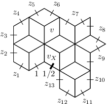 (b)
(c)
(b)
(c)
and suppose . Hence the set . The value is obtained by maximising over all edge-boundary pairs . Let be the vertex that is a neighbour to both and . Since , the boundary edge between and has colour 1 in every edge-boundary pair . An edge-boundary pair is therefore uniquely specified by the colour of its remaining boundary edges. Figure 9(a) illustrates an arbitrary edge-boundary pair , where boundary edges are labelled with their colour (). Thus, in order to maximise over all , we could loop through all combinations of the colours and compute for each such combination. This process will take very long. Next we explain how to speed up the process.
By computing for many colourings of the boundary, one quickly makes the observation that only some particular colourings of the boundary result in a large value of . For other colourings, tends to be rather small. For example, it turns out that if are all colour 1, then will be rather small regardless of the remaining colours . Thus, setting the colours to 1 is a “bad” choice if we want to maximise . From this observation we conclude that if we can filter out certain “bad” colourings of the boundary then we could speed up the process of finding the maximum value .
We “split” the extended region into two extended regions and . Figure 9(b) and (c) illustrate and , respectively. The two regions share the vertices in the split. In this case it is vertex and , both labelled in the figure. Let be the edge-boundary pair such that , and the boundary edges receive the same colours as in . Boundary edges that are introduced from the split are given colour 0. Let be the edge-boundary pair defined similarly to but with . Figure 9(b) and (c) illustrate and .
Let be the colouring of such that for and . Recall from Section 5 that for , denotes the number of proper -colourings in such that . For two colours we now define to be the number of proper -colourings in such that and , where is the second vertex in the split. Thus,
Let be the colouring of such that and for . For two colours we define to be the number of proper -colourings in such that and . We define similarly for the edge-boundary pair . It follows that
and hence
With colours, we have
| (7) |
Note that the colours specify the quantity , and specify the quantity . In order to maximise over edge-boundary pairs , we could consider all combinations of the colours and use Equation (7). There are such combinations, so considering them all will take very long. Now, consider two different sets of the six colours . For , let be the value of for the first set of colours, and let be the value of for the second set of colours. Suppose
| (8) |
for all , and . Then we have from Equation (7) that can only get smaller if we take instead of . In other words, there is no point considering the colours specified by the second set of colours when maximising . This observation suggests that we loop through all combinations of colours and compare each pair of combinations like in Equation (8). We only keep the sets of colours that cannot be ruled out in some pairwise comparison like the second set above. This gives us a collection of colours that turns out to be much smaller than the collection of all sets of colours. Similarly we obtain a collection of colours for the right part of the region. In order to find which colours that maximise we combine with . That is, we use Equation (7) to compute for each set of colours in with each set of colours in .
The technique of splitting regions and filtering out boundary colourings that are guaranteed not to maximise has a huge impact on the running time of the program. On a fairly powerful home-PC as of year 2006, it takes about two days to to obtain all 9440 values .
8.2 Constructing an -set
We describe how to construct an -set. Let be the extended region in Figure 10(a)
(a)
 (b)
(c)
(b)
(c)

(d)
(e) (f)
(f)
with some combination of labels “in” and “out” on the vertices. From we will derive 5-tuples that are added to a set . By considering all possible combinations of labels “in” and “out” on the vertices of , we construct the -set . We describe the process by first giving a concrete example.
Fix an “in/out”-labelling of the vertices of the extended region . Let be the value such that is an extended subregion of . Note that the extended regions , , are defined such that there is exactly one value for which this is true. Figure 10(b) shows the largest possible and Figure 10(c) shows the overlapping of and . We see from this figure that only some of the vertices of define . Similarly to how the extended region is obtained from , let be the three unique values such that is obtained from by the overlapping in Figure 10(d), is obtained from by the overlapping in Figure 10(e), and is obtained from by the overlapping in Figure 10(f). It is possible that neighbours of vertex in Figure 10(d)–(f) are labelled “out”, meaning that some of the extended regions might not exist. If this is the case we define and . For example, if the vertex to the left of vertex in Figure 10(d) is “out” then cannot exist and hence .
Suppose is an edge-boundary pair such that and are matching with respect to edge . Then . For and any two distinct colours such that , suppose is the extended edge-boundary pair that is constructed recursively in the tree . If then . We will now be more precise about the sets of edge-boundary pairs and incorporate the sets .
Suppose without loss of generality that and , and for some . Suppose the extended region in Figure 11(a)
(a)  |
(e)  |
(i) |
| , , | , , | , , |
| , | , | , |
(b)  |
(f)  |
(j) |
(c)  |
(g)  |
(k)  |
| (d) | (h)  |
(l) |
is an extended subregion of . Suppose that the colour of the edge between and in Figure 11(a) has colour in and . Then and hence . From Figure 11(a) we see that the extended region in Figure 4(b) is an extended subregion of . Hence belongs to or (or both). The crucial observation here is that if and only if . This follows from the fact that and hence there is a discrepancy at only when the colour is drawn from in the coupling . We therefore conclude that . Thus, . For and we see in Figure 11(a) that these edge-boundary pairs belong to either or . However, we are unable to tell exactly to which of the two sets these edge-boundary pairs belong. We therefore assume that any combination of the two sets is possible. The 3-tuples listed in Figure 11(a) indicate to which possible sets the edge boundary pairs , and belong. That is, a 3-tuple means that , and .
Let be the set of edge-boundary pairs such that is an extended subregion of and . Then for every . Remember that we have assumed above that . Let be the value such that is the set that minimises over all . If the minimiser is not unique, let be the smallest among the minimisers. Now, for each 3-tuple in Figure 11(a) we add the following 5-tuple to the set : .
Summing it all up, we construct the set as follows. First take an extended region . From we uniquely derive the sets , , and . If is an extended subregion of then we consider two values of : and . If is an extended subregion of then we also consider two values of : and . Now suppose . The twelve cases in Figure 11 cover all possible combinations of the sets to which the recursively constructed edge-boundary pairs , and belong. More precisely, if then Figure 11(a)–(d) apply. if then Figure 11(e)–(h) apply. if or then Figure 11(i)–(l) apply. From and the value of , we uniquely derive the set to which belongs. For each 3-tuple in the relevant case in Figure 11, we add the following 5-tuple to the set : . If the value of in a 3-tuple is 0 then . By considering every possible extended region and every possible value of (two values per region ), we construct a set that is an -set.
References
- [1] D. Achlioptas, M. Molloy, C. Moore, and F. Van Bussel. Sampling grid colorings with fewer colours. In LATIN 2004: Theoretical Informatics, volume 2976 of Lecture Notes in Computer Science, pages 80–89. Springer, 2004.
- [2] D. Aldous. Random walks on finite groups and rapidly mixing Markov chains. In Seminar on Probability, XVII, volume 986 of Lecture Notes in Mathematics, pages 243–297. Springer, 1983.
- [3] R. Bubley and M. Dyer. Path coupling: a technique for proving rapid mixing in Markov chains. In FOCS ’97: Proceedings of the 38th Symposium on Foundations of Computer Science, pages 223–231. IEEE Computer Society Press, 1997.
- [4] P. Diaconis and L. Saloff-Coste. Comparison theorems for reversible Markov chains. Annals of Applied Probability, 3(3):696–730, 1993.
- [5] P. Diaconis and D. Stroock. Geometric bounds for eigenvalues of Markov chains. Annals of Applied Probability, 1(1):36–61, 1991.
- [6] M. Dyer, L. A. Goldberg, M. Jerrum, and R. Martin. Markov chain comparison. Probability Surveys, 3:89–111, 2006.
- [7] M. Dyer and C. Greenhill. Random walks on combinatorial objects. In Surveys in Combinatorics, volume 267 of London Mathematical Society Lecture Note Series, pages 101–136. Cambridge University Press, 1999.
- [8] M. Dyer, A. Sinclair, E. Vigoda, and D. Weitz. Mixing in time and space for lattice spin systems: a combinatorial view. Random Structures and Algorithms, 24(4):461–479, 2004.
- [9] H.-O. Georgii. Gibbs measures and phase transitions. de Gruyter Studies in Mathematics 9. Walter de Gruyter & Co., Berlin, Germany, 1988.
- [10] H.-O. Georgii, O. Häggström, and C. Maes. The random geometry of equilibrium phases. Phase Transitions and Critical Phenomena, 18:1–142, 2001.
- [11] L. A. Goldberg, M. Jalsenius, R. Martin, and M. Paterson. Improved mixing bounds for the anti-ferromagnetic potts model on . LMS Journal of Computation and Mathematics, 9:1–20, 2006.
- [12] L. A. Goldberg, R. Martin, and M. Paterson. Strong spatial mixing with fewer colours for lattice graphs. SIAM Journal on Computing, 35(2):486–517, 2005.
- [13] M. Jalsenius. Strong spatial mixing and rapid mixing with 9 colours for the triangular lattice. arXiv:0706.0489v1 [math-ph], 2007.
- [14] M. Jerrum. A very simple algorithm for estimating the number of -colorings of a low-degree graph. Random Structures and Algorithms, 7(2):157–165, 1995.
- [15] M. Jerrum. Counting, Sampling and Integrating: Algorithms and Complexity. Birkhäuser, Basel, Switzerland, 2003.
- [16] M. Jerrum, L. Valiant, and V. Vazirani. Random generation of combinatorial structures from a uniform distribution. Theoretical Computer Science, 43:169–188, 1986.
- [17] F. Martinelli. Lectures on Glauber dynamics for discrete spin models. In Lectures on Probability Theory and Statistics (Saint-Flour, 1997), volume 1717 of Lecture Notes in Mathematics, pages 93–191. Springer, 1999.
- [18] M. Molloy. Very rapidly mixing Markov chains for 2-colourings and for independent sets in a 4-regular graph. Random Structures and Algorithms, 18(2):101–115, 2001.
- [19] D. Randall and P. Tetali. Analyzing Glauber dynamics by comparison of Markov chains. Journal of Mathematical Physics, 41:1598–1615, 2000.
- [20] J. Salas and A. D. Sokal. Absence of phase transition for antiferromagnetic Potts models via the Dobrushin uniqueness theorem. Journal of Statistical Physics, 86(3–4):551, 1997.
- [21] A. Sinclair. Improved bounds for mixing rates of Markov chains and multicommodity flow. Combinatorics, Probability and Computing, 1:351–370, 1992.
- [22] E. Vigoda. Improved bounds for sampling colourings. Journal of Mathematical Physics, 41(3):1555–1569, 2000.
- [23] D. Weitz. Mixing in Time and Space for Discrete Spin Systems. PhD thesis, University of California, Berkley, 2004.
- [24] D. Weitz. Combinatorial criteria for uniqueness of Gibbs measures. Random Structures and Algorithms, 27(4):445–475, 2005.
- [25] D. Weitz. Counting independent sets up to the tree threshold. In STOC ’06: Proceedings of the 38th Annual ACM Symposium on Theory of Computing, pages 140–149. ACM Press, 2006.