Two-Dimensional Conformal Models of Space-Time and Their CompactificationThanks: On leave from Odessa University.
Abstract.
We study geometry of two-dimensional models of conformal space-time based on the group of Möbius transformation. The natural geometric invariants, called cycles, are used to linearise Möbius action. Conformal completion of the space-time is achieved through an addition of a zero-radius cycle at infinity. We pay an attention to the natural condition of non-reversibility of time arrow in order to get a correct compactification in the hyperbolic case.
1. Introduction
The ideas of symmetries and invariants were introduced by Galileo centuries ago but still are central to many branches of theoretical physics. In a mathematical version they are known as Erlangen program delivered by F. Klein and influenced by S. Lie, which is mistakenly limited to geometry often [8, 10].
Study of space-time geometry based on the group of conformal maps was very fruitful, see for example [14]. It is worth o consider a two-dimensional conformal space-time [4, 5] as it illustrates many general features.
In this paper we briefly overview an approach [3, 9, 10] to conformal space-time geometry associated with the Möbius action of group—the group of matrices of real entries with the unit determinant. We emphasise natural conformal invariants—called cycles [15]—and their rôle in conformal completion of the space-time. The usage of hypercomplex (dual and double) numbers along with complex ones gives a unified description for all model. We also stress some natural physical requirements omitted in [4]. Although all mentioned bits appeared in literature in different places before their gathering under one roof seems to be new and quite fruitful. Moreover it opens a straightforward possibility for a multidimensional generalisation, which is outlined at the end of paper.
2. Möbius transformations and cycles
A left action of group on a real line is given by linear-fractional or Möbius maps:
| (2.1) |
This action makes sense also as a map of complex, double and dual numbers [10], [15, Suppl. C], which have the form , with different values of the imaginary unit square: , or correspondingly. Although the arithmetic of dual and double numbers are different from the complex ones, e.g. they have divisors of zero, there are many properties in common.
Three possible values , and of will be refereed here as elliptic, parabolic and hyperbolic cases respectively. All three together will be abbreviated as EPH. One of the reason is that circles, parabolas and (equilateral) hyperbolas are invariant under the corresponding Möbius transformation.
The common name cycle [15] is used to denote the corresponding conic sections (as well as straight lines as their limits) in the respective EPH case. More precisely a generic cycle is the set of points defined for all values of by the equation
| (2.2) |
We denote this space by for a generic , specialised EPH cases will be written as , , .
A common method is to declare objects under investigations (cycles in our case, functions in functional analysis, etc.) to be simply points of some bigger space. Equation (2.2) (and the corresponding cycle) is defined by a point from a projective space , since for a scaling factor the point defines the same equation (2.2). We call the cycles space and refer to the initial as the points space.
In order to get a connection with Möbius action (2.1) we arrange numbers into the matrix [3, 9, 10]
| (2.3) |
with a new imaginary unit and an additional parameter usually equal to . The values of is , or independently from the value of . The matrix (2.3) is the cornerstone of (extended) Fillmore–Springer–Cnops construction (FSCc) [3, 6, 9, 10].
The FSCc is significant for conformal maps because it intertwines Möbius action (2.1) on cycles with a linear map by matrix similarity:
| (2.4) |
3. Invariants of cycles: algebraic and geometric
For matrices (and thus cycles) there are only two essentially different invariants under similarity (2.4) (and thus under Möbius action (2.1)): the trace and the determinant. However due to projective nature of the cycle space the a non-zero values of trace or determinant are relevant only if cycles are suitable normalised.
For example, if we may normalise the quadruple to with highlighted cycle’s centre. Moreover in this case is equal to the square of cycle’s radius [9, 11]. Another normalisation is used in [6] to get a nice condition for touching circles.
We still get important characterisation even with non-normalised cycles, e.g., invariant classes (for different ) of cycles are defined by the condition . Such a class is parametrises only by two real number and as such is easily attached to certain point of . For example, the cycle with , drawn elliptically represent just a point , i.e. (elliptic) zero-radius circle. The same condition with in hyperbolic drawing produces a null-cone originated at point :
i.e. a zero-radius cycle in hyperbolic metric. Note that in all cases the zero-radius cycle consists of non-invertible points (divisor of zero) in . We denote a zero-radius cycle centred at by .
Remark 3.1.
In general for every notion there is nine possibilities: three EPH cases (three values of ) in the cycle space times three EPH realisations (three values of ) in the point space.
We should clarify the relation between our nine cases and nine Cayley-Klein geometries [5, 4, 15]. Our parameter describes the signature of the point space: (which is ) and thus coincides with parameter from [5, 4]. However our parameter is different from used in [5, 4]. The later describes constant curvature whereas all our spaces are “flat” (their curvature is zero). Our parameter describes metric of the cycle spaces : if it is different from then this measure “non-locality” of our geometry. This notion cannot be embedded in any way into the Riemann geometry since it is “local” from the definition.
The most expected relation between cycles is based on the following Möbius invariant “inner product” build from a trace of product of two cycles as matrices (cf. with GNS construction to make a Hilbert space out of -algebra [1]):
| (3.1) |
The next standard move is to define -orthogonality of two cycles as vanishing of their inner product:
| (3.2) |
For the case of , i.e. when geometries of the cycles and points spaces are both either elliptic or hyperbolic, such an orthogonality is the standard one, defined in terms of angles between tangent lines in the intersection points of two cycles. However in the remaining seven () cases the innocent-looking definition (3.2) brings unexpected relations between cycles [9].
One can easy check the following orthogonality properties of the zero-radius cycles defined in the previous section [9]:
- (1)
Since zero-radius cycles are self-orthogonal (isotropic) ones.
- (2)
A cycle is -orthogonal to a zero-radius cycle if and only if passes through the -centre of .
4. Conformal compactification by zero-radius cycles
(a) (b)
(b)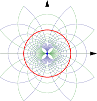
(c) (d)
(d)
Likewise an association of points of with cycles (2.2) in overlooked exceptional values. For example, the image of , which is corresponds to the equation , is not a valid conic section in . We also did not investigate yet accurately singular points of the Möbius map (2.1). It turns out that both questions are connected.
One of the standard approaches [12, § 1] to deal with singularities of the Möbius map is to consider projective coordinates on the plane. Since we have already a projective space of cycles, we may use it as a model for compactification which is even more appropriate. The identification of points with zero-radius cycles, discussed above, plays an important rôle here.
More specifically we represent the zero-radius cycle at infinity by the point denoted it by . The following results on can be found in [9]:
- (1)
is the image of the zero-radius cycle at the origin under reflection (inversion) into the unit cycle , see blue cycles in Fig. 1(b)-(d).
- (2)
The following statements are equivalent
- (a)
A point belongs to the zero-radius cycle centred at the origin;
- (b)
The zero-radius cycle is -orthogonal to zero-radius cycle ;
- (c)
The inversion in the unit cycle is singular in the point ;
- (d)
The image of under inversion in the unit cycle is orthogonal to .
If any from the above is true we also say that image of under inversion in the unit cycle belongs to zero-radius cycle at infinity.
- (a)


(a) (b) (c)
Now we are going to discuss conformal compactification of spaces which makes action of Möbius map (2.1) on it non-singular at any point. Our description will be based on the concept of zero-radius cycle.
It is very well known that in the elliptic case the conformal compactification is done by addition to a point at infinity, which is the elliptic zero-radius cycle. However in the parabolic and hyperbolic cases the singularity of the Möbius transform is not localised in a single point—the denominator is a zero divisor for the whole zero-radius cycle. Thus in each EPH case the correct compactification is made by the union .
It is common to identify the compactification of the space with a Riemann sphere. This model can be visualised by the stereographic projection, see [2, § 18.1.4] and Fig. 2(a). A similar model can be provided for the parabolic and hyperbolic spaces as well, see [4] and Fig. 2(b),(c). Indeed the space can be identified with a corresponding surface of the constant curvature: the sphere (), the cylinder (), or the one-sheet hyperboloid (). The map of a surface to is given by the polar projection, see [4, Fig. 1] and Fig. 2(a)-(c). These surfaces provide “compact” model of the corresponding in the sense that Möbius transformations which are lifted from by the projection are not singular on these surfaces.
However the hyperbolic case has its own caveats which may be easily oversight, cf. [4]. A compactification of the hyperbolic space by a light cone (which the hyperbolic zero-radius cycle) at infinity will indeed produce a closed Möbius invariant object. However it will not be satisfactory for some other reasons, physical in particular, which explained in the next subsection.
5. Non-invariance of the upper half-plane
The important difference between the hyperbolic case and the two others is that in the elliptic and parabolic cases the upper halfplane in is preserved by Möbius transformations from . However in the hyperbolic case any point with can be mapped to an arbitrary point with .
The lack of invariance in the hyperbolic case has many important consequences in seemingly different areas, for example:

- Geometry:
-
is not split by the real axis into two disjoint pieces: there is a continuous path (through the light cone at infinity) from the upper half-plane to the lower which does not cross the real axis (see -like curve joined two sheets of the hyperbola in Fig. 4(a)).
- Physics:
-
There is no Möbius invariant way to separate “past” and “future” parts of the light cone, see [14, § III.4] for a detailed discussion of this effect and implications in the four-dimensional Minkowski space-time. More precisely it it may be stated as follows: there is a continuous family of Möbius transformations reversing the arrow of time. For example, the family of matrices , provides such a transformation. Fig. 3 illustrates this by corresponding images for eight subsequent values of .
- Analysis:
-
There is no a possibility to split space of function into a direct sum of the Hardy type space of functions having an analytic extension into the upper half-plane and its non-trivial complement, i.e. any function from has an “analytic extension” into the upper half-plane in the sense of hyperbolic function theory, see [7].
(a) (b)
(b)
(a) the “upper” half-plane; (b) the unit circle.
All the above problems can be resolved in the following way [7, § A.3]. We take two copies and of , depicted by the squares and in Fig. 4 correspondingly. The boundaries of these squares are light cones at infinity and we glue and in such a way that the construction is invariant under the natural action of the Möbius transformation. That is achieved if the letters , , , , in Fig. 4 are identified regardless of the number of primes attached to them. The corresponding model through a stereographic projection is presented on Fig. 5, compare with Fig. 2(c).

This aggregate denoted by is a two-fold cover of . The hyperbolic “upper” half-plane in consists of the upper halfplane in and the lower one in . A similar conformally invariant infinite-fold cover of the Minkowski space-time was constructed in [14, § III.4] in connection with the red shift problem in extragalactic astronomy. A suitable modification of our double cover of two-dimensional space can be designed for the conformal version of the four-dimensional Minkowski space-time.
The similar construction should be also applied to the conformal version of the hyperbolic unit disk [9]. It is the image of the hyperbolic upper-half plane under the Cayley transform defined by the matrix . We define it in as follows:
It can be shown that is conformally invariant and has a boundary —two copies of the unit circles in and . We call the (conformal) unit circle in . Fig. 4(b) illustrates the geometry of the conformal unit disk in in comparison with the “upper” half-plane.
6. Conclusions and discussions
This paper discusses conformal geometry of elliptic, parabolic and hyperbolic two dimensional space-time in term of complex, dual and double numbers and associated Möbius transformations. We identify cycles (i.e. conics of the matching type) as natural invariant objects of the conformal geometries and associate zero-radius cycles with points of the space-time. A conformal compactification of the space-time is uniformly achieved by addition the zero-radius cycle at infinity. Two other methods (group-theoretical approach and stereographic projection) were used in [4, 5].
However in the hyperbolic case the compactification requires more consideration. In order to forbid a conformal map which revert time-arrow on the space-time we need to consider (at least) a double cover of the space-time. Such a model still can be realised through a suitable stereographic projection.
It is possible that cycles have a deeper physical meaning along with the geometrical one. It may worth to explore this side of result from [9].
To conclude the discussion we mention a possibility of a higher dimensions generalisation. Using Clifford algebras one can define [3, 13] the Vahlen–Liouville group of matrices which transform mapping (pseudo)-spheres into (pseudo)-spheres by Möbius transformations, where is (pseudo)-Euclidean space of signature . For the Minkowski space-time the similar construction can use quaternions instead of the corresponding Clifford algebra. In higher dimensions our parameter will be replaced by the corresponding signature of the bilinear form defining the metric. However degenerate bilinear forms seem not be considered in this context so far.
Acknowledgement: I am grateful to the anonymous referee for valuable suggestions which help to improve this paper.
References
- [1] William Arveson. An Invitation to C*-algebras. Springer-Verlag, 1976.
- [2] Marcel Berger. Geometry. II. Universitext. Springer-Verlag, Berlin, 1987. Translated from the French by M. Cole and S. Levy.
- [3] Jan Cnops. An introduction to Dirac operators on manifolds, volume 24 of Progress in Mathematical Physics. Birkhäuser Boston Inc., Boston, MA, 2002.
- [4] Francisco J. Herranz and Mariano Santander. Conformal compactification of spacetimes. J. Phys. A, 35(31):6619–6629, 2002. E-print: arXiv:math-ph/0110019.
- [5] Francisco J. Herranz and Mariano Santander. Conformal symmetries of spacetimes. J. Phys. A, 35(31):6601–6618, 2002. E-print: arXiv:math-ph/0110019.
- [6] A. A. Kirillov. A Tale on Two Fractals. 2006. (To appear).
- [7] Vladimir V. Kisil. Analysis in or the principal function theory. Complex Variables Theory Appl., 40(2):93–118, 1999. E-print: arXiv:funct-an/9712003. MR # 2000k:30078.
- [8] Vladimir V. Kisil. Meeting Descartes and Klein somewhere in a noncommutative space. In A. Fokas, J. Halliwell, T. Kibble, and B. Zegarlinski, editors, Highlights of Mathematical Physics, pages 165–189. AMS, 2002. E-print: arXiv:math-ph/0112059. MR # 2005b:43015.
- [9] Vladimir V. Kisil. Elliptic, parabolic and hyperbolic analytic function theory–1: Geometry of invariants. 2005. E-print: arXiv:math.CV/0512416. preprint LEEDS–MATH–PURE–2005–28.
- [10] Vladimir V. Kisil. Starting with group. 2006. E-print: arXiv:math.GM/0607387. preprint LEEDS–MATH–PURE–2006–11.
- [11] Vladimir V. Kisil. Fillmore–Springer–Cnops constructions implemented in GiNaC. Adv. Appl. Clifford Algebr., 17(1):59–70, 2007. updated full text and source files: E-print: arXiv:cs.MS/0512073.
- [12] Peter J. Olver. Classical invariant theory, volume 44 of London Mathematical Society Student Texts. Cambridge University Press, Cambridge, 1999.
- [13] Ian R. Porteous. Clifford algebras and the classical groups, volume 50 of Cambridge Studies in Advanced Mathematics. Cambridge University Press, Cambridge, 1995.
- [14] Irving Ezra Segal. Mathematical Cosmology and Extragalactic Astronomy. Academic Press [Harcourt Brace Jovanovich Publishers], New York, 1976. Pure and Applied Mathematics, Vol. 68.
- [15] I. M. Yaglom. A simple non-Euclidean geometry and its physical basis. Springer-Verlag, New York, 1979. An elementary account of Galilean geometry and the Galilean principle of relativity, Heidelberg Science Library, Translated from the Russian by Abe Shenitzer, With the editorial assistance of Basil Gordon.