Fluctuation properties of the TASEP with periodic initial configurationThanks: Technische Universität München, e-mail: praehofer@ma.tum.deThanks: Chiba University, e-mail: sasamoto@math.s.chiba-u.ac.jp
Abstract
We consider the joint distributions of particle positions for the continuous time totally asymmetric simple exclusion process (TASEP). They are expressed as Fredholm determinants with a kernel defining a signed determinantal point process. We then consider certain periodic initial conditions and determine the kernel in the scaling limit. This result has been announced first in a letter by one of us [34] and here we provide a self-contained derivation. Connections to last passage directed percolation and random matrices are also briefly discussed.
1 Introduction
Continuous time TASEP. The totally asymmetric simple exclusion process (TASEP) is one of the simplest interacting stochastic particle systems. Its particles are on the lattice of integers, , with at most one particle at each site (exclusion principle). The dynamics of the TASEP is defined as follows. Particles jump on the neighboring right site with rate provided that the site is empty. This means that jumps are independent of each other and take place after an exponential waiting time with mean , which is counted from the time instant when the right neighbor site is empty.
On the macroscopic level the particle density, , evolves deterministically according to the Burgers equation [32]. Therefore a natural question is to focus on fluctuation properties and on large deviations, which exhibit rather unexpected features. The fluctuations of the integrated particle current and in the positions of particles are two faces of the same coin as to be discussed later.
The fluctuations of particle positions are sensitive to the initial conditions. For example, one can consider particles initially positioned every second site, i.e., on . Another possibility would be to consider the stationary measure of the same density as initial condition, which is Bernoulli with density . The scaling exponents for particle positions fluctuations are the same for the two initial conditions. However, the limiting distribution differ: as we will see, in the first case it is the GOE Tracy-Widom of random matrices [41] which differs from the stationary case [12]. Thus it is of interest to understand which class of initial conditions leads to the same limit distribution.
The first result in this direction has been obtained for the step initial condition. To be precise, denote by the position of particle at time , where the ’s are integers labelling the particles from right to left. The step initial condition is then , . It has been studied by Johansson [15] by means of a growth model. In terms of the TASEP, the quantity analyzed is the large time asymptotic fluctuations of the position of a given particle. For any fixed , the fluctuation of are asymptotically governed by the GUE Tracy-Widom distribution, , namely there are some and such that
| (1.1) |
The distribution first appeared in the context of the Gaussian Unitary Ensemble (GUE) of random matrices as the distribution of the largest eigenvalue in the limit of large matrix dimension [40].
A natural question is to ask how the positions of different particles are correlated, i.e., one considers for fixed but large time the process . To illustrate known results we focus at , but the same holds with different numerical coefficients for , 11 1 We choose because then the term linear in disappears in (1.2), (1.3), and (1.6).. (1.1) tells us that the fluctuations live on a scale and it turns out that the position of two particles are, on the scale, non-trivially correlated over a distance of order . The exponents and are indeed the ones of the KPZ universality class [18], to which the TASEP belongs. Indeed, Johansson [16] proves a functional limit theorem in a discrete-time setting. Its continuous-time version writes
| (1.2) |
where is known as the Airy process, first discovered in the PNG model under droplet growth [29].
Besides the step initial condition explained above, at least two other situations are of particular interest. One is the stationary initial condition, for which the two-point function of the TASEP is analyzed in [12]. The second one has deterministic initial conditions leading to a macroscopically uniform density, thus called flat initial conditions. The simplest realization is to set , .
In [34] an important new result has been obtained, making possible the asymptotic analysis for such initial conditions. First of all, as expected by universality, the position of a particle has fluctuations governed by the GOE Tracy-Widom distribution, [41]. This result is a combination of [34, 11] and states
| (1.3) |
More importantly, in [34] the analogue of the Airy process for flat initial conditions, which we denote by , is identified. It is a marginal of the signed determinantal point process with the extended kernel (1.4). Here signed refers to the non-positiveness of the measure (it does not define a probability measure). Explicitly, let and let be the one-dimensional Laplacian; then
| (1.4) |
or, equivalently as shown in Appendix A,
| (1.5) |
This is in complete analogy with the Airy process , which is a marginal of the determinantal point process defined by the extended Airy kernel.
In Theorem 2.1 we provide a derivation of the fact that the joint distribution of particle positions is given by the Fredholm determinant of a kernel. This is a general result which is then applied to the flat initial conditions , , see Theorem 2.2. The proper rescaling of particle positions is
| (1.6) |
With this rescaling, in the limit of large time , the kernel converges to as shown in Theorem 2.3. There we show pointwise convergence. In a forthcoming paper [3] we will analyze a discrete time version of the TASEP and strengthen our result to the convergence of the Fredholm determinants. Such a stronger convergence would imply the convergence of (1.6) to in the sense of finite-dimensional distributions.
As a remark we want to point out that, while periodic initial condition does not seem to be accessible by previously known techniques, with the new construction both step and periodic initial conditions can be analyzed. The technique used so far is the reduction of the model to a determinantal point process via the Robinson-Schensted-Knuth correspondence. For further references and details on determinantal point processes we refer the reader to surveys [22, 14, 37, 17] and the lecture notes [38].
Reformulation of the result. The TASEP integrated current at position and time , , is the number of particles which jumped from site to site during the time interval . Let us label by the right-most particle starting at position . Then . Thus the result of this paper translates directly to the integrated currents.
The TASEP can be mapped to last passage percolation on with i.i.d. exponentially distributed random variables , . is the waiting time of particle number to jump from position to . There is a slight switch in the point of view. For the TASEP one considers the particle positions at fixed time , while in last passage percolation, one studies the last passage time from the origin to points of a given lattice domain . These two points of view are closely connected. They can be regarded as taking different cross sections in the Bernoulli cone [27]. The problem considered in [15] is the point-to-point last passage percolation, which corresponds to the step initial condition for the TASEP. Flat initial conditions correspond to the point-to-line percolation.
Finally, the same last passage percolation model can be seen as a one-dimensional growth model [33, 15], called discrete polynuclear growth model, which serves as a discretized model for KPZ growth [18]. KPZ growth is discussed in the books [2, 23] but for a recent exposition of KPZ universality see [27].
Universality issue. The TASEP also has discrete time versions. One of these is the parallel update rule (see the review [36]) and it is given as follows. At each time step particles jump to the neighboring right site with probability , provided the target site is empty. The jumps occurs independently and simultaneously. There are two interesting limits of the discrete-time TASEP, namely and . The continuous-time TASEP is obtained by setting the time-unit to and then take . The limit yields the so-called polynuclear growth (PNG) model, see e.g. Section 2.1.5 of [9]. There, one has a height function on a one-dimensional substrate, and flat initial condition for the TASEP translates to growth starting with , also called flat PNG.
By universality the process is expected to appear in the discrete-time TASEP and the PNG model as well. Universality has been confirmed for step initial conditions and the corresponding PNG model with droplet growth [16, 29]. Moreover, for flat initial conditions, the limit process should be independent on the initial particle spacing. Results in a discrete-time version of the TASEP with different initial spacing will be presented in [3].
For the flat PNG model, it is known [1, 28] that the height at one fixed point is GOE Tracy-Widom distributed in the limit of large time . Thus, on the basis of the result for the TASEP with alternating initial conditions, see Theorem 2.3, we can conjecture the behavior of the flat PNG model.
Conjecture 1.
The properly rescaled height function of the PNG model with flat initial conditions converges, in the large time limit, to the process .
The scaling exponents are the same and the coefficients can be determined by matching with the PNG droplet case.
Finally, let us discuss the connection to random matrices. For the TASEP with the step initial condition, the one-point asymptotic distribution is the GUE Tracy-Widom distribution, , and the whole limit process is the Airy process . The derivation uses an extension of the model to a multi-layer version. The Airy process arises also for a GUE matrix diffusion, the so-called Dyson’s Brownian Motion [6]. The motion of the properly rescaled largest eigenvalue converges to the Airy process. The connection extends to finitely many of the largest eigenvalues which have the same limiting behavior as the first top layers in the multi-layer PNG model.
For the TASEP with flat initial condition, the one-point distribution is the GOE Tracy-Widom distribution and the limit process is . At this point it is tempting to conjecture that the evolution of the largest eigenvalue of a matrix which follows Dyson’s Brownian Motion has the same limiting behavior as the surface height for flat PNG, namely the process. The correspondence at the level of top eigenvalues for GOE and the top layers of the multi-layer flat PNG at a fixed position has been proven in [8], making the conjecture even more plausible. Knowing the analogue of the Airy process for random growth with flat initial conditions one can guess the result for Dyson’s Brownian Motion [6].
Conjecture 2.
The evolution of the largest eigenvalue of matrices for Dyson’s Brownian Motion converges, in the limit and properly rescaled, to the process .
Again, the prefactors for the scaling can be easily calculated by matching the known one-point distributions and the behavior of joint distributions at short distances. This conjecture concerns only the largest eigenvalue and with this approach we are unable to make a conjecture for the other eigenvalues.
To make Conjecture 2 more transparent, we explain it in the simpler case of the two-matrix model. There, one considers two real symmetric matrices, and , with joint distribution
| (1.7) |
where and . Let and be the largest eigenvalues of and . These eigenvalues fluctuate on a scale of order and are non-trivially correlated if one chooses . Then Conjecture 2 means that, properly rescaled, the joint distribution of and converges to the two-point joint distribution of the process in the limit.
We also refer to the surveys on the question of universality in mathematics and physics [5] and on connections between different models, including random matrices [10].
Outline. The paper is organized as follows: In Section 2 we state the main result. In Section 3 the kernel of the signed determinantal point process describing the joint particle distributions is derived. The kernel involves an orthogonalization which is carried out in Section 4 for the case of alternating initial conditions. In Section 5 we prove the convergence of the properly rescaled kernel to the kernel . In Appendix A we explain how the compact form of the kernel is derived, and in Appendix B we explain how the orthogonalization can be carried out using classical Charlier orthogonal polynomials.
Acknowledgment
P.L. Ferrari would like to thank H. Spohn for useful discussions and for suggesting the compact form of the kernel obtained during our previous work [11]. A. Borodin was partially supported by the NSF grant DMS-0402047 and the CRDF grant RIM1-2622-ST-04. The work of T. Sasamoto is partly supported by the Grant-in-Aid for Young Scientists (B), the Ministry of Education, Culture, Sports, Science and Technology, Japan.
2 Model and results
In this paper we consider the continuous-time totally asymmetric simple exclusion process (TASEP) on . At any given time , every site can be occupied at most by one particle. Thus a configuration of the TASEP can be described by . is called the occupation variable of site , which is defined by if site is occupied and if site is empty.
The dynamics of the TASEP is defined as follows. Particles jumps on the neighboring right site with rate provided that the site is empty. This means that jumps are independent of each other and are performed after an exponential waiting time with mean , which starts from the time instant when the right neighbor site is empty. More precisely, let : be a function depending only on a finite number of ’s. Then the backward generator of the TASEP is given by
| (2.1) |
Here denotes the configuration with the occupations at sites and interchanged. The semigroup is well-defined as acting on bounded and continuous functions on . is the transition probability of the TASEP [21].
Joint distributions
Let us start at time with particles at positions . Then the main result is the joint distribution of any subset of these particles at time . It turns out that it can be described by a signed determinantal point process, where signed refers to the non-positiveness of the measure.
Theorem 2.1.
Let be the indices of out of the particles. The joint distribution of their positions is given by
| (2.2) |
where . is the extended kernel with entries
| (2.3) |
where
| (2.4) |
| (2.5) |
and the functions , , form a family of polynomials of degree satisfying
| (2.6) |
The path in the definition of is any simple loop, anticlockwise oriented, which includes the pole at but not the one at .
The dependence on the set is hidden in the definition of the ’s and the ’s but is omitted, since the set is fixed in the following.
Alternating initial configuration
Now we consider alternating initial configuration, namely
| (2.7) |
The alternating initial configuration can be obtained by taking particles around the origin, for example at positions , and then taking the limit . In Lemma 4.1 we do the orthogonalization, i.e., construct ’s which satisfy (2.6) for this special case, from which the kernel is obtained.
Theorem 2.2.
Let particle with label start at , . At time , the particles are at positions . The kernel (2.3) for the alternating initial configuration is given by
| (2.8) |
where is any simple loop, anticlockwise oriented, which includes the pole at but do not include .
Scaling limit
The particle density is and since particles jump to the right with rate provided the site is empty, the mean speed of the particles is . Let us number the particles from right to left with as reference point, i.e., , . Then the particles which at time are close to are the particles with numbers close to . From universality we know also that the scaling exponent for fluctuations should be and the one for spatial correlations should be . Therefore, the scaling limit to be considered is
| (2.9) |
Remark: The scaling exponents for this model are determined by the requirement that there is a non-trivial limit. The numerical factor in front of is chosen so that the single-time kernel has a simple form, . The numerical factors for the terms are set in such a way that the propagator in (1.4) is generated by the Laplacian without additional prefactors. Universality argument is not needed to obtain the result, but it is useful to predict the correct answer.
In Section 5 we carry out the asymptotic analysis for the pointwise convergence of the kernel, with the following result.
Theorem 2.3 (Pointwise convergence of the kernel).
In this paper we do not perform the asymptotic analysis necessary to get convergence of the Fredholm determinants. We will do the complete analysis in a discrete-time version of the TASEP in a forthcoming paper [3], from which the continuous time limit follows as a corollary. Nevertheless, it is instructive for the reader to see the implications of the convergence of the Fredholm determinant.
Let be the process with -point joint distributions at given by
| (2.11) |
where . The convergence of Fredholm determinant would then imply
| (2.12) |
with the convergence understood in the sense of finite-dimensional distributions.
3 Signed determinantal point process
In this section we prove Theorem 2.1. Consider the TASEP with particles starting at time at positions . The first step is to obtain the probability that at time these particles are at positions , which we denote by
| (3.1) |
This function has been determined before using Bethe-Ansatz method [35].
Lemma 3.1 (Schütz [35]).
The transition probability has a determinantal form
| (3.2) |
with
| (3.3) |
where is any simple loop oriented anticlockwise which includes and .
This representation of the transition probability was utilized to study the current fluctuations in [24, 30]. To study the joint distribution, we need a decomposition of given in the next lemma. This decomposition is obtained using only the recurrence relation
| (3.4) |
and its integrated form
| (3.5) |
Actually, (3.5) comes from (3.4) and the fact that fast enough. The other property needed to obtain Theorem 2.1 is the following. Comparing (2.5) and (3.3), we have
| (3.6) |
for . Notice that, for , (3.3) defining has actually only one pole at . We then get the relation
| (3.7) |
which translates into
| (3.8) |
In the definition of the ’s in Theorem 2.1, the path includes only the pole at the origin, exactly because we need (3.8) to hold also for .
Lemma 3.2.
Let us denote , . Then
| (3.9) |
where the sum is over the following set
| (3.10) |
See Figure 1 for a graphical representation of .

This lemma is actually more general as shown in [34]. By applying just the recursion relation (3.5) the domain of summation in Lemma 3.2 would be instead of . The reduction of the summation domain to uses only the antisymmetry of the determinant. Thus the same holds for any antisymmetric function . It might be interesting in other applications, so we state it explicitly.
Lemma 3.3.
Let an antisymmetric function of . Then, whenever has enough decay to make the sums finite,
| (3.11) |
where
| (3.12) |
and the positions being fixed.
Proof of Lemma 3.2. The proof consists in applying the property (3.5) iteratively and using the multilinearity of the determinants. From Lemma 3.1 we have
| (3.13) |
The first step is to rewrite the last row as
| (3.14) |
The second step is to apply the same procedure to the last and second to last rows, which become
| (3.15) |
and
| (3.16) |
respectively. At this point we have
| (3.17) |
The determinant is antisymmetric in the variables , therefore the contribution of the symmetric part of the summation domain of is zero. Since , the symmetric part of the domain is , thus the contribution coming from the last sum is zero.
We iterate the same procedure. More precisely, for , we apply (3.5) to the last rows. The new summing variable for the last row is denoted by , the second last row , and so on. Finally, we can delete the sums over the symmetric domain in . In this way we get the result
| (3.18) |
∎
This is the decomposition used in [34]. The integrations variables can be interpreted as the positions of particles labelled by at time . For example, is the trajectory of particle , see also Figure 2. This is just a mathematical construction which should not to be confused with the real TASEP particles and the natural time in the TASEP positions, which at this stage is just the fixed parameter . At time there are particles at positions . At time , they jump to a randomly uniformly chosen position satisfying with the st particle added at position . Then the weight of a configurations of ’s is given by
| (3.19) | |||
where we set . The products of determinants in (3.19) might look complicated. However, one can verify that whenever some of the ’s do not satisfy the inequalities of , then at least one of the determinant vanishes. On the other hand, if the set of ’s belongs to , then each determinant has value .
The form of the weight suggests that the correlation functions could be determinantal. It is like to have a Lindström-Gessel-Viennot (LGV) scheme [42], see [39] for a nice exposition, with a sort of reservoir of particles at and at each time-step a new particle is introduced. The LGV scheme is a sort of generalization on a class of directed graphs of the Karlin-McGregor result for diffusions [19]. Determinantal form of correlation functions appeared in different contexts [7, 13, 25, 4, 16]. Although we do not use the LGV scheme in the proof, it might be interesting for the reader to see how the weight (3.19) can be described in this framework. The situation given by the weight (3.19) corresponds to the limit of the system with fixed number of particles illustrated in Figure 2. As , the extra particles are not seen, they goes to in a sort of reservoir.

The proof of Theorem 2.1 is an application of the following Lemma, which is proven by using the framework of [4].
Lemma 3.4.
Assume we have a signed measure on given in the form,
| (3.20) |
where are some “virtual” variables and is a normalization constant. If , then the correlation functions are determinantal.
To write down the kernel we need to introduce some notations. Define
| (3.21) |
where , and, for ,
| (3.22) |
Set . Then the functions
| (3.23) |
are linearly independent and generate the -dimensional space . Define a set of functions spanning defined by the orthogonality relations
| (3.24) |
for .
Under Assumption (A): , for some , , the kernel takes the simple form
| (3.25) |
Remarks: Without Assumption (A), the correlations functions are still determinantal but the formula is modified as follows. Let be the dimensional matrix defined by . Then
| (3.26) | |||||
The analogue of the determinantal representation (3.2) for particle-dependent hopping rates has been recently obtained [31]. Lemma 3.4 might be applied in this context too.
Proof of Lemma 3.4. We apply Proposition 1.2 of [4] and we try to stick as much as possible to the notations therein. Let, for , denote the space of , , and let be the space on which our measure (3.20) is defined. Let be the matrix with entries
| (3.27) |
and
| (3.28) |
Then the weight (3.20) is proportional to the determinant of
| (3.29) |
We are interested in the measure on only, thus we change the ordering by putting the variables at the beginning. Let us define the matrix by
| (3.30) |
and the matrix by
| (3.31) |
Then the weight (3.20) is proportional to a suitable symmetric minor of , with
| (3.32) |
By Proposition 1.2 of [4], the point-measure on is determinantal with correlation kernel given by
| (3.33) |
provided that the partition function . With the decomposition of , we have a block decomposition of as
| (3.34) |
with , , and equal to without the first line and column of the block representation (3.32). Let , then (see, e.g., Lemma 1.5 of [4]) the kernel is given by
| (3.35) |
was already computed in Lemma 1.5 of [4], with the result
| (3.36) |
where
| (3.37) |
Thus the block of is . Next, we have
| (3.38) |
and
| (3.39) |
Therefore the block of the correlation kernel is given by
| (3.40) |
Using (3.21) one gets . Moreover by (3.22) we have
| (3.41) |
It remains to evaluate the last part of (3.40). For the following matrix we have
| (3.42) |
Notice that the functions in (3.42) form a basis of . Thus we can define a matrix which does a change of basis to , namely
| (3.43) |
We multiply this equation by and obtain
| (3.44) |
In particular, we have . Let us define the matrix
| (3.45) |
Then
| (3.46) |
Assume the condition (B): for . Then we get the simple form of the kernel, (3.25), of the Lemma. However, this is not always the case. For , we obtain using (3.22),
| (3.47) |
Thus we can write for some matrix . By multiplying on both sides by the condition (B), we see that (B) is equivalent to
| (3.48) |
for all and for all , and for all . But the functions form a basis of , thus (B) is fulfilled iff for all . Thus (B) is equivalent to the condition is an upper-diagonal matrix.
Assume upper diagonal for some . This is verified for where . Then by (3.47) for , and is still upper-diagonal iff
| (3.49) |
because . Finally, the orthogonal relations (3.24) imply that , which is Assumption (A) of the Lemma. ∎
Proof of Theorem 2.1. It consists in an application of Lemma 3.4, with
| (3.50) |
and
| (3.51) |
An important point is that in (3.3) the functions ’s are defined by an integral enclosing and . At this stage, we have only functions ’s for . In this case, as mentioned around (3.6), is actually not a pole, thus the weight (3.19) and the weight (3.20) with the above replacements are proportional. The definition of the ’s using only one pole fit exactly in the framework of Lemma 3.4. In fact, by (3.8), we have the composition rule
| (3.52) |
which gives (3.22) by iterations. In our setting, if we sum up all the variables , we get a Vandermonde determinant in the variables ’s. Thus the space of Lemma 3.4 is generated by and are polynomials of order at most . A simple computation using (2.5) leads to
| (3.53) |
which, together with (3.24) leads to . Thus we have a determinantal system with kernel (3.25), which can be rewritten as
| (3.54) |
Since in this paper we explain the detail of the derivation in [34], it is useful to point out a difference. There one does not obtain directly as in Theorem 2.1. There the one-time transition becomes and the representation (3.3) has to be used instead. The final form of the kernel (eq. (13) in [34]) comes from splitting the contribution from the pole at and the remainder. In the geometric picture, it corresponds to have the conjugate LGV graph with reservoir of particles at instead of at . ∎
4 Orthogonalization
In order to get the kernel for the alternating initial configuration, i.e., for the case where particles initially occupy exactly the sublattice , we start with a finite number of particles, . In the second step we will focus on the region where the -dependence vanishes. In this way we will get the kernel for the system we actually are interested in.

Consider the case where at time there are particles placed every second site centered around the origin, see Figure 3, namely
| (4.1) |
From Theorem 2.1, the kernel is known once the orthogonalization is carried out. Here we state the result and a short proof. In Appendix B we explain a constructive way of obtaining needed functions using Charlier orthogonal polynomials.
Lemma 4.1.
The functions and have the following integral representations. Let . Then
| (4.2) |
and
| (4.3) |
where is an anticlockwise simple loop enclosing only the pole at .
Proof.
We have
| (4.4) |
Then (3.3) leads directly to (4.2). Next we prove that (4.3) satisfy the orthogonality relation (3.24). Since for , we have
| (4.5) | |||||
provided that the integration domain satisfy . The last sum gives
| (4.6) |
Thus (4.5) has a simple pole at , and once the integral over is computed, we get
| (4.7) |
The final step is a change of variable. Let . Then
| (4.8) |
and the integral is again around . Thus we get
| (4.9) |
∎
Once the orthogonalization is made, we determine the kernel of Theorem 2.2.
Proof of Theorem 2.2. We need to derive the formula for the first term (the main part) of the kernel. For convenience, we first shift the integrating variable of to go around by setting . This leads to
| (4.10) |
with . We start with particles at positions , . The main term in the kernel writes, with ,
| (4.11) |
provided that the integration paths satisfies (a) and (b) is not inside the contour . To obtain this expression we first take the finite sum over inside the integrals, and secondly we extend it to . This can be done since the sum is absolutely summable because of (a) and we do not create new poles inside the integration contours because of (b). For example, we can set by and take to be a contour with small enough.
To obtain the kernel for the alternating initial configuration we focus on the ’s far enough from the right-most particle so that the system in the considered region becomes independent of the fact that we have only a finite number of particles. This is obtained when , i.e., whenever is not anymore a pole. This condition is satisfied for any fixed (i.e., around the origin) and any finite time by taking large enough. In fact, it corresponds to taking in . In this case we are left with one simple pole at . Denote , then and the main part of the kernel becomes, for any ’s as ,
| (4.12) |
Finally, by relabelling the particles we obtain (2.8). ∎
5 Asymptotic analysis
In this section we do the asymptotic analysis for the alternating initial conditions and prove Theorem 2.3. Just to remind, the scaling limit we have to consider is
| (5.1) |
Proof of of Theorem 2.3. The pointwise limit of the first term is quite easy to obtain. Let us set , , and . Then we have to compute
| (5.2) |
We simply use . Since for is a bounded set, as , we have that
| (5.3) |
and by replacing back the expressions of and we get,
| (5.4) |
Next we analyze the second of the kernel (2.8) multiplied by . This writes
| (5.5) |
with
| (5.6) |
To do a steep descent analysis we first have to find the stationary points of . Simple computations lead to
| (5.7) |
which has a double zero at . Moreover,
| (5.8) |
The steep descent path used for the analysis, shown in Figure 4, is given by with
| (5.9) | |||||
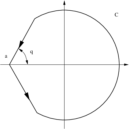
Let us verify that is actually a steep descent path22 2 For an integral , we say that is a steep descent path if (1) is maximum at some : for and (2) is monotone along except, if is closed, at a single point where reaches its minimum.. On ,
| (5.10) |
Therefore the real part of is stationary only at and the maximum is at , the minimum at . By symmetry we need to check only on . We find
| (5.11) |
which is strictly negative except at where is zero. Thus is a steep descent path.
Consider now the piece of the path . Let us denote . Then since is a steep descent path,
| (5.12) | |||||
for some (in our case, ). The precise expression of is
| (5.13) |
For the integral on we can apply Taylor development. On we have , , and we obtain
| (5.14) |
where the error terms are uniform for in a bounded set. Set to be the expressions without the error terms, and similarly : . Then
| (5.15) |
To estimate the second integral, we use the inequality . Thus
| (5.16) | |||||
for some which can be made as small as desired by choosing small enough. At the integration boundary the leading term is . This easily implies that the integral remains bounded as . Now we do the change of variable . The and . The rest of the integral is for some constants , since the function do not contains the error terms. The integrand is then times and the integral is on . The dominates the integral for large . Thus remains finite in the limit. Therefore the above estimate of the error term becomes .
The final step is to compute . Extending to we only make an error of order for some and this leads to the integration along the path . Therefore
| (5.17) | |||||
The change of variable leads then to
| (5.18) | |||||
Finally we use an Airy function representation
| (5.19) |
to obtain the final result
| (5.20) |
∎
Appendix A Compact form for the extended kernel
In this Appendix we show that the entries of the compact form of the kernel (1.4) agree with (2.10). Let us introduce some notations. Let be the multiplication operator by the position, be the differentiation operator, and let be the Laplacian. On Schwarz test functions ,
| (A.1) |
Moreover, denote by the operator with kernel and the Airy operator .
We will apply Baker-Campbell-Haussdorf formula. If and for some constant , then
| (A.2) |
from which follows, for ,
| (A.3) |
Moreover, we will use the property of Airy functions
| (A.4) |
We collect some useful properties in the following lemma.
Lemma A.1.
- 1)
Commutation relations: , ,
- 2)
,
- 3)
and ,
- 4)
.
Proof.
What we have to compute explicitly is . From 4) of Lemma A.1 we have
| (A.7) |
The last part can be rewritten as
| (A.8) |
by (A.2) with and . Then using (A.3) with and we obtain
| (A.9) |
Plugging this back into (A.7) we have
| (A.10) |
Then we apply 3) of Lemma A.1, namely , and we exchange the order of and because are both symmetric and apply 4) of Lemma A.1. This results into
| (A.11) |
Explicitly
| (A.12) |
Thus we showed how the second term in (1.4) leads to the corresponding one in (1). It remains the first one, , for . This is just the one-dimensional heat kernel, for which it is well known that (see e.g. [26])
| (A.13) |
Appendix B Charlier polynomials
In this Appendix we explain a constructive method to do the orthogonalization. Let be the Charlier polynomial of degree . They are orthogonal polynomials with respect to the weight on given by
| (B.1) |
which are traditionally normalized via
| (B.2) |
or, equivalently, . They can be expressed in terms of hypergeometric functions
| (B.3) |
and satisfy the recurrence relation
| (B.4) |
From the generating function of the Charlier polynomials
| (B.5) |
one gets the integral representation
| (B.6) |
For a good reference on orthogonal polynomials, see [20].
It is not too difficult to see that the functions defined in Lemma 4.1 can be expressed in terms of the Charlier orthogonal polynomials as
| (B.7) |
Using the recurrence relation (B.4) repeatedly we obtain
| (B.8) |
where the entries of the matrix are
| (B.9) |
Notice that is not a square matrix. From this it follows that the polynomials which satisfy
| (B.10) |
are given by
| (B.11) |
where by we mean the -entry of the inverse of the square matrix obtained by restricting to the first indices. The first main difficulty is to obtain the inverse of . After some work we could determine it, namely
| (B.12) |
with the identification and the convention that the RHS of (B.12) is zero when .
References
- [1] J. Baik and E.M. Rains, Limiting distributions for a polynuclear growth model with external sources, J. Stat. Phys. 100 (2000), 523–542.
- [2] A.L. Barabási and H.E. Stanley, Fractal concepts in surface growth, Cambridge University Press, Cambridge, 1995.
- [3] A. Borodin, P.L. Ferrari, and M. Prähofer, Fluctuations in the discrete TASEP with periodic initial configurations and the Airy1 process, preprint: arXiv:math-ph/0611071 (2006).
- [4] A. Borodin and E.M. Rains, Eynard-Mehta theorem, Schur process, and their Pfaffian analogs, J. Stat. Phys. 121 (2005), 291–317.
- [5] P. Deift, Universality for mathematical and physical systems, arXiv:math-ph/0603038 (2006).
- [6] F.J. Dyson, A Brownian-motion model for the eigenvalues of a random matrix, J. Math. Phys. 3 (1962), 1191–1198.
- [7] B. Eynard and M.L. Mehta, Matrices coupled in a chain. I. Eigenvalue correlations, J. Phys. A 31 (1998), 4449–4456.
- [8] P.L. Ferrari, Polynuclear growth on a flat substrate and edge scaling of GOE eigenvalues, Comm. Math. Phys. 252 (2004), 77–109.
- [9] P.L. Ferrari, Shape fluctuations of crystal facets and surface growth in one dimension, Ph.D. thesis, Technische Universität München, http://tumb1.ub.tum.de/publ/diss/ma/2004/ferrari.html, 2004.
- [10] P.L. Ferrari and M. Prähofer, One-dimensional stochastic growth and Gaussian ensembles of random matrices, Markov Processes Relat. Fields 12 (2006), 203–234.
- [11] P.L. Ferrari and H. Spohn, A determinantal formula for the GOE Tracy-Widom distribution, J. Phys. A 38 (2005), L557–L561.
- [12] P.L. Ferrari and H. Spohn, Scaling limit for the space-time covariance of the stationary totally asymmetric simple exclusion process, Comm. Math. Phys. 265 (2006), 1–44.
- [13] P.J. Forrester, T. Nagao, and G. Honner, Correlations for the orthogonal-unitary and symplectic-unitary transitions at the hard and soft edges, Nucl. Phys. B 553 (1999), 601–643.
- [14] J. Ben Hough, M. Krishnapur, Y. Peres, and B. Virag, Determinantal processes and independence, preprint: arXiv:math/0503110 (2005).
- [15] K. Johansson, Shape fluctuations and random matrices, Comm. Math. Phys. 209 (2000), 437–476.
- [16] K. Johansson, Discrete polynuclear growth and determinantal processes, Comm. Math. Phys. 242 (2003), 277–329.
- [17] K. Johansson, Random matrices and determinantal processes, Mathematical Statistical Physics, Session LXXXIII: Lecture Notes of the Les Houches Summer School 2005 (A. Bovier, F. Dunlop, A. van Enter, F. den Hollander, and J. Dalibard, eds.), Elsevier Science, 2006, pp. 1–56.
- [18] K. Kardar, G. Parisi, and Y.Z. Zhang, Dynamic scaling of growing interfaces, Phys. Rev. Lett. 56 (1986), 889–892.
- [19] S. Karlin and L. McGregor, Coincidence probabilities, Pacific J. 9 (1959), 1141–1164.
- [20] R. Koekoek and R.F. Swarttouw, The Askey-scheme of hypergeometric orthogonal polynomials and its q-analogue, arXiv:math.CA/9602214 (1996).
- [21] T.M. Liggett, Stochastic interacting systems: contact, voter and exclusion processes, Springer Verlag, Berlin, 1999.
- [22] R. Lyons, Determinantal probability measures, Publ. Math. Inst. Hautes Etudes Sci. 98 (2003), 167–212.
- [23] P. Meakin, Fractals, scaling and growth far from equilibrium, Cambridge University Press, Cambridge, 1998.
- [24] T. Nagao and T. Sasamoto, Asymmetric simple exclusion process and modified random matrix ensembles, Nucl. Phys. B 699 (2004), 487–502.
- [25] A. Okounkov and N. Reshetikhin, Correlation function of Schur process with application to local geometry of a random 3-dimensional Young diagram, J. Amer. Math. Soc. 16 (2003), 581–603.
- [26] B.K. Øksendal, Stochastic differential equations, 5th ed., Springer Verlag, Berlin, 1998.
- [27] M. Prähofer, Stochastic surface growth, Ph.D. thesis, Ludwig-Maximilians-Universität, München, http://edoc.ub.uni-muenchen.de/archive/00001381, 2003.
- [28] M. Prähofer and H. Spohn, Universal distributions for growth processes in dimensions and random matrices, Phys. Rev. Lett. 84 (2000), 4882–4885.
- [29] M. Prähofer and H. Spohn, Scale invariance of the PNG droplet and the Airy process, J. Stat. Phys. 108 (2002), 1071–1106.
- [30] A. Rákos and G. Schütz, Current distribution and random matrix ensembles for an integrable asymmetric fragmentation process, J. Stat. Phys. 118 (2005), 511–530.
- [31] A. Rákos and G. Schütz, Bethe Ansatz and current distribution for the TASEP with particle-dependent hopping rates, Markov Process. Related Fields 12 (2006), 323–334.
- [32] F. Rezakhanlou, Hydrodynamic limit for attractive particle systems on , Comm. Math. Phys. 140 (1991), 417–448.
- [33] H. Rost, Non-equilibrium behavior of a many particle system: density profile and local equilibrium, Z. Wahrsch. Verw. Gebiete 58 (1981), 41–53.
- [34] T. Sasamoto, Spatial correlations of the 1D KPZ surface on a flat substrate, J. Phys. A 38 (2005), L549–L556.
- [35] G.M. Schütz, Exact solution of the master equation for the asymmetric exclusion process, J. Stat. Phys. 88 (1997), 427–445.
- [36] G.M. Schütz, Exactly solvable models for many-body systems far from equilibrium, Phase Transitions and Critical Phenomena (C. Domb and J. Lebowitz, eds.), vol. 19, Academic Press, 2000, pp. 1–251.
- [37] A. Soshnikov, Determinantal random fields, Encyclopedia of Mathematical Physics (J.-P. Francoise, G. Naber, and T. S. Tsun, eds.), Elsevier, Oxford, 2006, pp. 47–53.
- [38] H. Spohn, Exact solutions for KPZ-type growth processes, random matrices, and equilibrium shapes of crystals, Physica A 369 (2006), 71–99.
- [39] J.R. Stembridge, Nonintersecting paths, Pfaffians, and plane partitions, Adv. Math. 83 (1990), 96–131.
- [40] C.A. Tracy and H. Widom, Level-spacing distributions and the Airy kernel, Comm. Math. Phys. 159 (1994), 151–174.
- [41] C.A. Tracy and H. Widom, On orthogonal and symplectic matrix ensembles, Comm. Math. Phys. 177 (1996), 727–754.
- [42] G. Viennot, Une forme géométrique de la correspondence de Robinson-Schensted, Combinatoire et Représentation du Groupe Symétrique, Lecture Notes in Mathematics, vol. 579, Springer-Verlag, Berlin, 1977, pp. 29–58.